Article

Deep Cerebellar Transcranial Direct Current Stimulation of the Dentate Nucleus to Facilitate Standing Balance in Chronic Stroke Survivors—A Pilot Study

1
Department of Biomedical Engineering, University at Buffalo, The State University of New York, Buffalo, NY 14260, USA
2
All India Institute of Medical Sciences, New Delhi 110029, India
3
Indian Institute of Technology Gandhinagar, Palaj 382355, India
*
Author to whom correspondence should be addressed.
Brain Sci. 2020, 10(2), 94; https://doi.org/10.3390/brainsci10020094
Submission received: 2 January 2020 / Revised: 22 January 2020 / Accepted: 4 February 2020 / Published: 10 February 2020
(This article belongs to the Special Issue Collection on Neural Engineering)

Abstract

:
Objective: Cerebrovascular accidents are the second leading cause of death and the third leading cause of disability worldwide. We hypothesized that cerebellar transcranial direct current stimulation (ctDCS) of the dentate nuclei and the lower-limb representations in the cerebellum can improve functional reach during standing balance in chronic (>6 months’ post-stroke) stroke survivors. Materials and Methods: Magnetic resonance imaging (MRI) based subject-specific electric field was computed across a convenience sample of 10 male chronic (>6 months) stroke survivors and one healthy MRI template to find an optimal bipolar bilateral ctDCS montage to target dentate nuclei and lower-limb representations (lobules VII–IX). Then, in a repeated-measure crossover study on a subset of 5 stroke survivors, we compared 15 min of 2 mA ctDCS based on the effects on successful functional reach (%) during standing balance task. Three-way ANOVA investigated the factors of interest– brain regions, montages, stroke participants, and their interactions. Results: “One-size-fits-all” bipolar ctDCS montage for the clinical study was found to be PO9h–PO10h for dentate nuclei and Exx7–Exx8 for lobules VII–IX with the contralesional anode. PO9h–PO10h ctDCS performed significantly (alpha = 0.05) better in facilitating successful functional reach (%) when compared to Exx7–Exx8 ctDCS. Furthermore, a linear relationship between successful functional reach (%) and electric field strength was found where PO9h–PO10h montage resulted in a significantly (alpha = 0.05) higher electric field strength when compared to Exx7–Exx8 montage for the same 2 mA current. Conclusion: We presented a rational neuroimaging based approach to optimize deep ctDCS of the dentate nuclei and lower limb representations in the cerebellum for post-stroke balance rehabilitation. However, this promising pilot study was limited by “one-size-fits-all” bipolar ctDCS montage as well as a small sample size.

1. Introduction

Cerebrovascular accidents (stroke) are the second leading cause of death and the third leading cause of disability worldwide (Global Health Estimates. Geneva, Switzerland: World Health Organization; 2012). Worldwide, 70% of strokes and 87% of both stroke-related deaths and disability-adjusted life years occur in low- and middle-income countries (LMIC) [1]. While the incidence of stroke is decreasing in the developed world [1], the incidence is increasing in India, an LMIC, due to demographic transition and a rapid shift in the socio-economic milieu. The estimated adjusted prevalence rate of stroke ranges from 84–262/100,000 in rural and 334–424/100,000 in urban India, and the incidence rate is 119–145/100,000 based on the recent population-based studies [2]. Thus, stroke constitutes a substantial socioeconomic burden on the patients, caregivers, and society in India [3,4]. The scarcity of trained rehabilitation clinicians, as well as the cost of clinic-based rehabilitation programs, can deter stroke survivors from undergoing regular post-stroke rehabilitation leading to further decline in their health conditions. Given the high prevalence and incidence of stroke in India, there is a need to investigate low-cost neurotechnologies to facilitate early post-stroke rehabilitation.
Early task-specific rehabilitation after stroke may drive functionally relevant beneficial neuroplastic changes in the brain where neuroplasticity is the ability of the central nervous system to respond to intrinsic or extrinsic stimuli by reorganizing its structure, function, and connections. Recent clinical studies in the USA on invasive deep brain stimulation of the cerebellum for post-stroke motor rehabilitation are based on the extensive reciprocal connectivity between the dentate nucleus and the wide swaths of cerebral cortex via the dentatothalamocortical and corticopontocerebellar tracts [5]. Dentate is a promising target for brain stimulation since it remains mostly unaffected by lesions [6], and deep brain stimulation of the cerebellum is proposed to ameliorate the known limitations to motor rehabilitation imposed by crossed cerebellar diaschisis. Here, the improvements in motor function are found paralleled by increased expression of markers of synaptic plasticity, synaptogenesis, and neurogenesis in the perilesional cortex. In this study, we investigated a low-cost non-invasive brain stimulation (NIBS) approach to the cerebellum [7,8] based on cerebellar transcranial direct current stimulation (ctDCS). ctDCS has been found to be a promising method to facilitate cerebellar functions [9] where it can improve locomotor adaptation [10] as well as postural recovery from disturbance by Achilles tendon vibration [11]. The conventional ctDCS electrode montages [12] most likely produce their effects by polarizing Purkinje cells [13], and its therapeutic effects are an adjunct to motor training [8]. In this study, we aimed to directly target the dentate nucleus with ctDCS which is the largest and most lateral of the four deep cerebellar nuclei and is known to be involved in planning and executing voluntary movements [14]. In fact, the dentate nucleus can affect motor as well as cognitive function [12] due to extensive reciprocal connectivity between the dentate nucleus and the wide swaths of the cerebral cortex. Since dentate receives proprioceptive information from the spinocerebellar tract via the inferior cerebellar peduncle and also receives planning and initiating voluntary movement-related information from the premotor and supplementary motor cortices so it can perform error computations (comparator function) relevant to maintain timing, balance, and equilibrium. Therefore, we postulate that subthreshold stimulation of the dentate nucleus can help generate appropriately timed burst activity [15] during standing balance functional reach tasks (FRT) using a human-machine interface (HMI) [16]. Our prior work on ctDCS optimization [7] showed that highly conductive cerebrospinal fluid can provide a path for the stimulation current to reach the depths of the vermis, and since the dentate nucleus is directly adjacent to the vermis and the roof of the fourth ventricle bilaterally so we aimed to directly target dentate nucleus with ctDCS to facilitate cued weight-shifting in chronic stroke survivors. Here, patient selection may be crucial for ctDCS as an adjunct to post-stroke balance rehabilitation, e.g., in patients where the cerebellum is without lesion and the cerebello-cerebral connectivity is intact, since stroke is a heterogeneous disease with different mechanisms and etiologies.
While non-invasive brain stimulation (NIBS) techniques, including tDCS, are increasingly used for the modulation of corticospinal excitability in humans by passing low electric currents through the brain, its treatment effects are rather inconsistent across studies [17,18]. Besides usability issues, one of the important factors contributing to the inconsistency is the lack of expertise in individualizing tDCS [17,18]. For example, ctDCS has shown promise in improving standing balance performance in small studies with fifteen patients with chronic stroke (>6 months post-stroke) [19] where exploration of optimal timing, dose, and the relation between qualitative parameters and clinical improvements are needed [19]. A recent study [20] showed that multiple sessions (three sessions of 20 min per week for two weeks) of simultaneous postural training with bilateral anodal ctDCS (not postural training or bilateral anodal ctDCS alone) was necessary to deliver therapeutic effects in older adults with high fall risk. However, due to heterogeneous brain lesions in stroke, subject-specific optimization of the ctDCS electric field using Magnetic Resonance Imaging (MRI) data and a computational pipeline [7] is important. We have shown that different ctDCS electrode montages affect different parts or lobules of the cerebellum [7,21], however, the related behavioral effects could not be determined in our prior works in the absence of patient data. In the current pilot study, we tested the usability and feasibility of a bipolar bilateral ctDCS in chronic (>6 months) stroke survivors where a group-averaged optimal bipolar bilateral ctDCS montage was developed based on subject-specific optimization across post-stroke participant MRI as well as based on a healthy MRI template. Usability testing with well-defined neuroimaging based customization outside of laboratory setting is necessary for strengthening remote patient care and monitoring for chronic stroke conditions. Here, heterogeneously lesioned brain regions after stroke present a challenge because of the alterations of current flow, which may require the development of individualized ctDCS electrode montage based on neuroimaging [7]. In this study, we selected stroke survivors with cerebral lesions but with an intact cerebellum so that the ctDCS electric field effects can be delivered via intact cerebellum [8]. We first optimized ctDCS with a whole head electrode montage using an age-appropriate human brain MRI template for the age-group of 55 to 59 years (https://jerlab.sc.edu/projects/neurodevelopmental-mri-database/) to select a reduced set of electrodes that were then used to optimize bipolar bilateral ctDCS montage based on the MRIs from our post-stroke participants.
Our computational modeling pipeline [7] and FRT evaluated a bipolar bilateral ctDCS montage to maximally (with electric field strength) target bilateral dentate nuclei (postulated to affect motor as well as cognitive function [12]) versus one optimized to uniformly target the leg area of the cerebellum (i.e., comparable electric field in X, Y, Z directions across lobules VII–IX) [7]. User experience due to 2 mA bipolar ctDCS were monitored by asking participants whether they experienced any of the following symptoms since the preceding treatment: scalp pain, headache, neck pain, dental pain, tingling, nausea, itching, burning sensation, skin redness, open lesion on skin, abnormal sleep, anxiety, difficulty concentrating, dizziness, impaired memory, altered mood, altered balance, impaired use of the unaffected side, or any other problem [22].

2. Materials and Methods

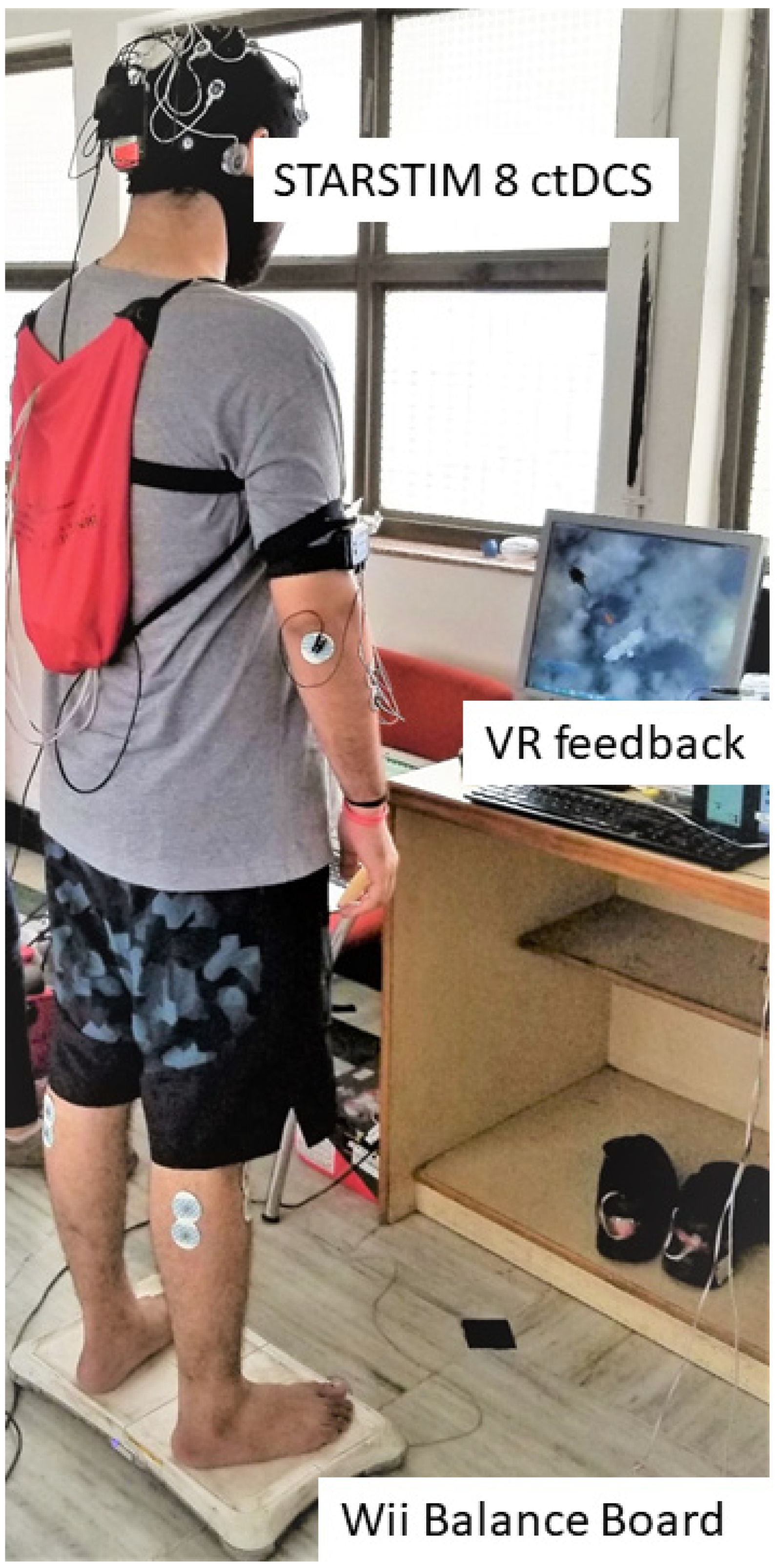
2.1. Experimental Setup and Study Design

Figure 1 shows the portable experimental setup for the clinical study in a low resource setting. The experimental setup consisted of a portable Wii Balance Board (WiiBB), a small form factor desktop PC with monitor for the VR-based balance training platform [23], and wireless STARSTIM 8 stimulator (Neuroelectrics, Spain) for cerebellar transcranial direct current stimulation (ctDCS). Based on Van de Winckel [22], the capacity building for the clinical study included: (1) ctDCS treatment design and supervision of ctDCS to facilitate VR-based FRT; (2) assessment of the stroke survivor’s capability to participate in VR-based FRT; (3) ongoing training procedures and materials including assessments of the stroke survivor using VR-based FRT; (4) simple and fail-safe electrode placement technique using a neoprene cap; (5) dose estimation based on computational modeling; (6) quantifying compliance by the rehabilitation specialist at the site (ctDCS device preparation, electrode saturation/placement, stimulation protocol), with corresponding corrective steps as required; (7) monitoring for treatment-emergent adverse effects; (8) procedures for discontinuation of a session or study participation including emergency failsafe procedures tailored to the treatment population’s level of need. The subject-specific ctDCS dose (Guideline 5) was simulated by the first author and confirmed by the last author based on our computational modeling pipeline [7] to reduce potential adverse events due to electric field spillover to the lesioned cerebral regions.
A convenience sample of ten male chronic (>6 months post-stroke) stroke subjects participated in the subject-specific MRI-based computational modeling [7]. Based on the assessment of the stroke survivor’s capability to participate in the VR-based FRT, only five subjects (listed in Table 1) completed both the interventions of ctDCS with pre/post FRT in a repeated-measure single-blind counterbalanced study. Two subjects could only attend a single intervention due to scheduling conflicts. Written informed consent was obtained from each participant, and the research protocol for this study was approved by the All India Institute of Medical Sciences New Delhi, India Institutional Review Board (IEC-129/07.04.2017).
During each session, chronic stroke participants performed FRT for 10 min for a baseline measure of the CoP target reach performance. During FRT [24,25,26], the participant was offered a VR-based target stimulus where CoP (from WiiBB) was mapped to the dynamic position of a VR cursor object that could be modulated to reach the VR target object using weight-shifts on the WiiBB. The details of the VR-based balance training platform are provided in Verma et al. [23]. Briefly, the subject needs to reach a peripheral VR target in the front or to the sides by weight shifting the CoP within a fixed time. Following baseline measure of the CoP target reach performance, 15 min of 2 mA bilateral ctDCS delivered using either of the two bipolar montages with a 1cm radius circular contralesional anode. The electrode locations were based on the Realistic volumetric Approach to Simulate Transcranial Electric Stimulation (ROAST) toolbox [27] and “unambiguously illustrated (UI) 10/5 system” [28] (illustrated in the head model in Figure 2), 1. PO9h–PO10h, and 2. Exx7–Exx8. Further details on computational modeling are provided in Section 2.3. FRT for 10 min was repeated after ctDCS intervention for a post-intervention measure of the CoP target reach performance.

2.2. Data Acquisition and Head Modeling

The head model was constructed using subject-specific MRIs from ten male stroke survivors (see Table 1) collected based on the research protocol which was approved by the All India Institute of Medical Sciences (AIIMS), New Delhi, India Institutional Review Board. All subjects were screened for their eligibility to be included in this neuroimaging study by the Department of Nuclear Magnetic Resonance (NMR) at AIIMS. MRI was performed by a 3 Tesla (Achieva or Ingenia, Philips Medical Systems) MR unit using a sixteen multichannel receiver head coil. The MR sequence consists following parameter: MPRAGE, 192 slices, matrix size = 240 × 220, Flip/Flop angle = 8/0, TR/TE = 8.0/3.7 [29,30].
For computational modeling and whole head electrode optimization (details provided in Section 2.3), an age-appropriate averaged (n = 73) human brain MRI template for the 55 to 59 years age-group was obtained online at https://jerlab.sc.edu/projects/neurodevelopmental-mri-database/ with the permission of Dr. John Richards. The subjects were all normal healthy adults with no history of neurological or psychiatric illness, head trauma with loss of consciousness, or current or past use of psycho-stimulant medications, cardiovascular disease, and no abnormal findings on the MRI [31]. Average age-group specific MRI template was nonlinearly registered to an average reference image using “Advanced Normalization Tools” (ANTS) [32]. This program provides symmetric normalization of the source volumes to the reference volumes. The data consisted of average (male and female) T1-weighted MRI for the head and brain, and segmenting priors for gray matter (GM), white matter (WM), and cerebrospinal fluid (CSF), from the Neurodevelopmental MRI Database [31,33,34,35,36]. The head model is shown in Figure A1 of Appendix B.
Tetrahedral volume mesh was created using the ROAST toolbox [27], which is a Matlab (Mathworks, MA, USA) script based on three open-source software; Statistical Parametric Mapping (SPM) [37], Iso2mesh [38], and getDP [39]. ROAST used SPM12 [40] to segment the head and the brain. After segmentation, five tissues were labeled for the tetrahedral volume mesh, namely, Scalp, Skull, Cerebrospinal Fluid (CSF), Gray Matter (GM), and White Matter (WM). These different brain tissues for the volume mesh were modeled as different volume conductors for finite element analysis (FEA) in the ROAST. Here, isotropic conductivity based on prior works was used for different brain tissues [30] which were (in S/m): Scalp = 0.465; Skull = 0.01; CSF = 1.654; GM = 0.276; WM = 0.126 [7,30,41,42]. A subject-specific cap fitted to the individual head model was created using the high-density 10-05 EEG locations [43], EGI net-based system (https://www.egi.com), and extra electrodes from ROAST [27] along with nine custom locations that were defined on the neck and the lower head.

2.3. Finite Element Analysis (FEA) for ctDCS Optimization Based on the MRI Template of 55 to 59 Years Old

Although multi (>2)-electrode montages can improve the focality and specificity [44] and can be delivered by our (expensive) stimulation device (STARSTIM 8, Neuroelectrics, Spain), however, we were limited by a 2-electrode bipolar montage so that the ctDCS montage can be translatable to low-cost (<$150) tDCS devices available in community setting (or, home-based) in India. Furthermore, whole head subject-specific MRI-based head modeling may not be feasible in a low-resource setting constrained by a lack of computing power so we aimed to identify a reduced set of electrodes optimized for ctDCS. Then, based on that reduced set of electrodes, we aimed to identify “one-size-fits-all” bipolar montage across our post-stroke subject group (n = 10) that can maximally (electric field strength) target bilateral dentate nuclei (postulated to affect motor as well as cognitive function [13]) or can uniformly (comparable electric field in X, Y, Z directions across lobules VII-IX) target the leg area of the cerebellum [7]. Therefore, the first step was to perform computational modeling across different available bipolar ctDCS montages and ctDCS optimization based on an age-appropriate averaged (n = 73) MRI template of the 55 to 59 years old. Here, tetrahedral volume meshing and the FEA was performed using the ROAST pipeline [27]. This pipeline provides a numerical tool to solve the required partial differential equations (PDE) to generate the transfer matrices necessary for the optimization [7]. Boundary condition was set to constant injection current (Neumann boundary condition). The electric field (EF) was modeled for ctDCS using five different montages.

2.3.1. Computational Modeling and Optimization Based on MRI Template of 55 to 59 Years Age-Group

(1) Celnik montage [13]: 5 cm × 5 cm anode was placed over the right cerebellum, 1 cm below, and 3 cm lateral to the inion (Iz, 10/10 EEG system). The 5 cm × 5 cm cathode was over the right buccinator muscle for ctDCS with 2 mA direct current.
(2) Manto montage [45]: 5 cm × 5 cm anode was placed over the right cerebellum, 1 cm below, and 3 cm lateral to the inion (Iz, 10/10 EEG system). The 5 cm × 5 cm cathode was on the contralateral supraorbital area (FP2, 10/10 EEG system) for ctDCS with 2 mA direct current.
(3) Extracephalic montage: 5 cm × 5 cm anode was placed over the right cerebellum, 1 cm below, and 3 cm lateral to the inion (Iz, 10/10 EEG system). The 5 cm × 5 cm cathode was on the right neck area for ctDCS with 2 mA direct current.
(4) Optimization for dentate nuclei: electrode location of one 3.14 cm2 (1 cm radius) circular anode and one 3.14 cm2 circular cathode was optimized using our computational pipeline [7] for 2 mA ctDCS. The details on the optimization process are presented next in Section 2.3.2.
(5) Optimization for bilateral lobules VII-IX: electrode location of one 3.14 cm2 (1 cm radius) circular anode and one 3.14 cm2 circular cathode was optimized using our computational pipeline [7] for 2 mA ctDCS. The details on the optimization process are presented next in Section 2.3.2.

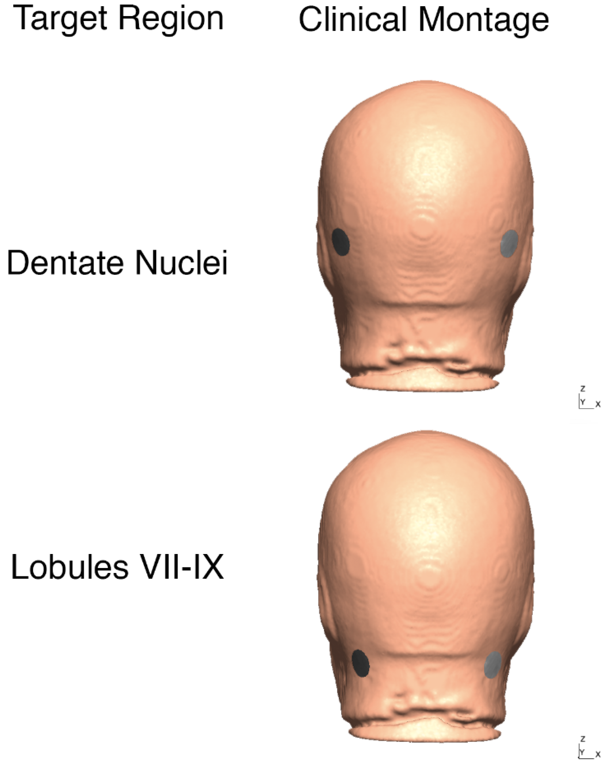
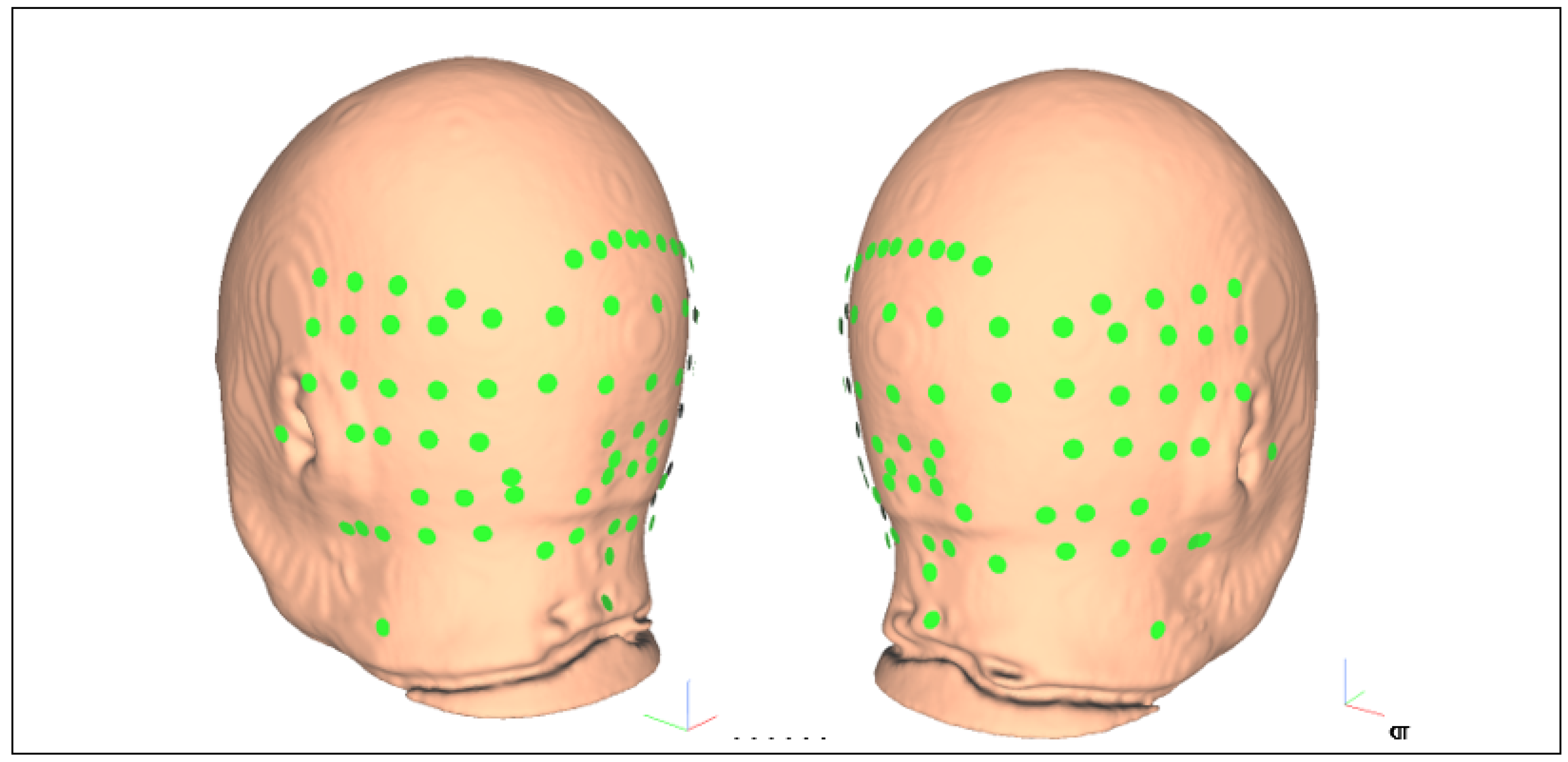
2.3.2. Cerebellar tDCS Optimization Using the Head Model for the Age Group of 55–59 Years

Finite element analysis (FEA) tools, including ROAST [27], can be used to solve the quasistatic approximation for Maxwell’s equation with a linear approximation of Ohm’s law in a purely resistive medium Ω So, we can write in a matrix form E = L I where E is the electric field vector ( E = [ E x   E y   E z ] ); x, y, z are 3D global Cartesian coordinates—see Figure 2) generated by the stimulation currents, I, applied at the scalp electrode array, and L is the ‘transfer matrix’ (or, ‘leadfield matrix’) that (columns) maps the electric field ( E = [ E x   E y   E z ] ); generated in the brain for an unit current applied to each of the stimulation electrodes [46] with a joint return electrode (‘Cz’ in our case [7]). Here, the headspace is discretized as a 3D finite element mesh and the discretized solution for E can be availed after FEA at the nodes (called the nodal values). With discretization, the transfer matrix, L, is a 3m × n size matrix for m nodes and n scalp stimulation current sources (excluding ‘Cz’), I. Therefore, the forward model can be written as, E = L I + e , where the 3m × n electric field vector, E , at any node, m, is a linear projection or mapping by the transfer matrix, L, of the stimulation current sources, I, with additive (environmental) noise, e. Here, usually m >> n, due to large (>10000) number of nodes, m, necessary to reduce numerical error in FEA [47] when compared to the number of electrode locations that available on the EEG cap (=429 in our case—See Appendix B: Table A2). In fact, the current applied at a finite-sized electrode (1cm circular electrode in our case) needs to be resolved to the nodes at the electrode-scalp interface, so one can also use uniformly distributed nodes at the scalp surface mesh for point current sources, I, to generate the ‘transfer matrix’ which can however drastically increase n and can make the system underdetermined requiring regularization as discussed next.
We can assume that the additive noise, e, is a multivariate Gaussian variable with zero mean and covariance matrix, C e , which is independent of I. The additive noise can be due to external electromagnetic sources (can be recorded on the scalp during the experiment) in the absence of any applied scalp stimulation current sources, I. The problem of finding appropriate stimulation currents, I R n , i.e., the vector of the unknown, for the multi-electrode array to shape the given nodal values of the electric field, E R 3 m , via the transfer matrix, L R 3 m × n , in presence of noise, e R 3 m , can be framed as a minimization problem with L2 regularization [48], I ^ = arg   min I ( ( E L I ) T C e 1 ( E L I ) + λ I 2 2 ) = L ( L T L + λ C e ) 1 E , where ( )T is the transpose of the matrix, λ is the penalization parameter to keep the stimulation currents, I ^ , small, and C e is the 3m × n noise covariance matrix. Here, the solution, I ^ , emphasizes stimulation current sources near the peak (target) electric field, E , which is driven by the norms of the columns of the transfer matrix, L. Here, L is usually very large and sparse as computed from FEA. Current sources for a superficial (near the scalp) brain target (peak electric field, E ) are desired to be near the peak electric field, E , in practice (e.g., to stay away from non-targeted lesions), therefore, dropping a scalp stimulation current source with the high norm of its corresponding column inc L will be detrimental. So, a forward selection approach to find the scalp stimulation current sources with the high norm of its corresponding L column can be applied to reduce the number of variables, i.e., the size of the vector I R n . We applied this approach to select the size of vector I R n that is appropriate for our cerebellar target (here, “superficiality” of the target is in terms of the resistivity of the medium where a similar target depth in a conductive medium will be more superficial than a resistive medium). We also assumed that the covariance matrix, C e , is an identity matrix, so I ^ = arg   min I ( ( E L I ) T ( E L I ) + λ I 2 2 ) can be framed as a convex optimization with constraints [49] where I ^ vector is the optimization variable. Here, convex optimization with constraints [49] is a powerful technique to minimize functions, f, that are convex, i.e., fx + βy) ≤ αf(x) + βf(y), for all x ,   y R n and all α ,   β R with α + β = 1, α ≥ 0, β ≥ 0. Convex optimization is not only applicable for least-square regression problem shown above but also for linear programming where the objective is to maximize the electric field, E , at the targeted nodes of the brain region based on a vector of weights, W R 3 m , i.e., I ^ = arg   max I ( W T L I ) . The ‘beamforming’ problem in array signal processing [46,50] based on the minimization of the total energy stored in an electric field constrained to a target electric field, E , at a volume is equivalent to the least-square problem (can be shown using Lagrange multipliers) [49].
In this study, we formulated two convex optimization problems [49] based on the head model for the age group of 55–59 years from the Neurodevelopmental MRI Database [31,33,34,35,36] (see Section 2.2 for details),
Objective 1: minimize the sum of squares of error between the desired electric field distribution, E , at the ankle/leg area of the cerebellum (i.e., bilateral cerebellar lobules VII-IX [7]) and the one generated by the stimulation currents, i.e., I ^ = arg   min I ( ( E L I ) T ( E L I ) ) = arg   min I E L I 2 , under the following constraints:
Total anodal current is equal to the cathodal current;
j = 1 n I i = 0
Total anodal and cathodal current magnitude is below a set threshold of 4 mA for safety and comfort (i.e., maximum anodal or cathodal current is 2 mA);
j = 1 n | x j | 4
This convex optimization problem was solved using CVX toolbox in MATLAB (Mathworks, Inc., MA, USA) to get an achievable uniform ( E x = E y = E z ) electric field at the cerebellar lobules related to the ankle/leg function [51], a.k.a, lobules VII-IX [7], that can then be scaled in practice by scaling the stimulation currents, I ^ , vector due to a linear system, E = L I .
Objective 2: maximize the electric field, E , at the dentate nuclei of the cerebellum, i.e., I ^ = arg   max I ( W T L I ) where W R 3 m is a vector of weights (with one for E x , E y , E z at the nodes of the dentate nuclei and zeros elsewhere), under the following constraints:
Total anodal current is equal to the cathodal current;
i = 1 n I i = 0
Total anodal and cathodal current magnitude is below a set threshold of 4 mA for safety and comfort (i.e., maximum anodal or cathodal current is 2 mA);
j = 1 n | x j | 4
This was solved using CVX toolbox in MATLAB (Mathworks, Inc., MA, USA) to get a maximum electric field at the dentate nuclei of the cerebellum, that can then be scaled in practice by scaling the stimulation currents, I ^ , vector due to a linear system, E = L I .
Possible electrode positions for stimulation current sources were defined for the whole head coverage (n = 429—see Appendix B: Table A2) by combining the high-density 10-05 EEG locations [43] with the EGI net-based system (https://www.egi.com) and extra electrodes from ROAST [27]. CLOS pipeline [7] was used to compute the ‘transfer matrix’, L, for each nodal location and direction of the electric field by combining 429 FEA simulations. In all the simulations, the voxel size was considered as 1mm3. In CLOS [7], the electric field, E , a vector can be mapped (i.e., A E = A L I ) using a spatially unbiased atlas template of the cerebellum and brainstem (SUIT) [52] for 34 SUIT parcellations (or, regions—see Appendix A: Table A1) and the non-cerebellar brain (i.e., total 35 regions) to the average electric field in the X, Y, and Z directions of the global coordinate system, i.e., mean Ex, mean Ey, mean Ez, in the 35 regions (where A is 105 × 3m mapping matrix). We divided the new transfer matrix, AL (reduced size and sparsity from L but easier to process in Matlab with limited desktop memory) into three 35 × 429 matrices, each for mean Ex, mean Ey, and mean Ez, as shown in Appendix C.

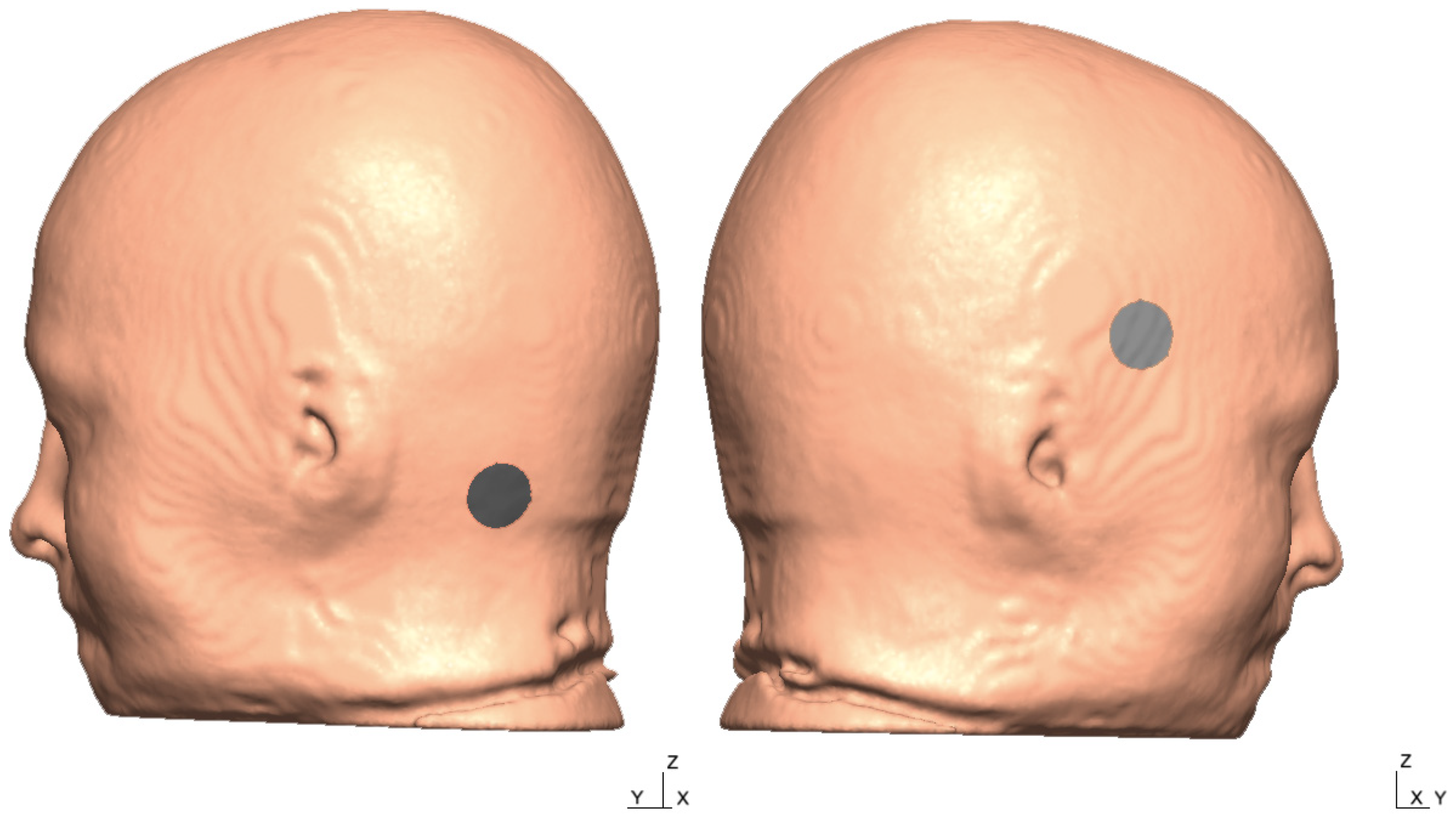
2.3.3. Computational Modeling for the Post-Stroke Subjects

Stroke survivors had lesions in the cerebral areas (primarily frontal lobe) so the bipolar electrodes needed to be limited to the scalp overlying the cerebellum and the neck. The L1 norm of the columns of these transfer matrices (from 55–59 years age-group MRI template) are shown in Figure A3, Figure A6 and Figure A9 for Ex, Ey, and Ez respectively in Appendix B along with a reduced set of electrodes (see Figure 3) found from the union of the electrode locations with high L1 norm from the three (Ex, Ey, and Ez) transfer matrices (see Table A3, Table A4 and Table A5 for Ex, Ey, and Ez respectively in Appendix C). Here, L1 norm of the non−cerebellar brain (row= 35) of the Ex, Ey, and Ez transfer matrices are lower than 0.12 compared to greater than 1 for the cerebellar brain (see Figure A4, Figure A7 and Figure A10 for Ex, Ey, and Ez respectively in Appendix C) so not affected significantly by the reduced set of electrodes (see Figure 3).

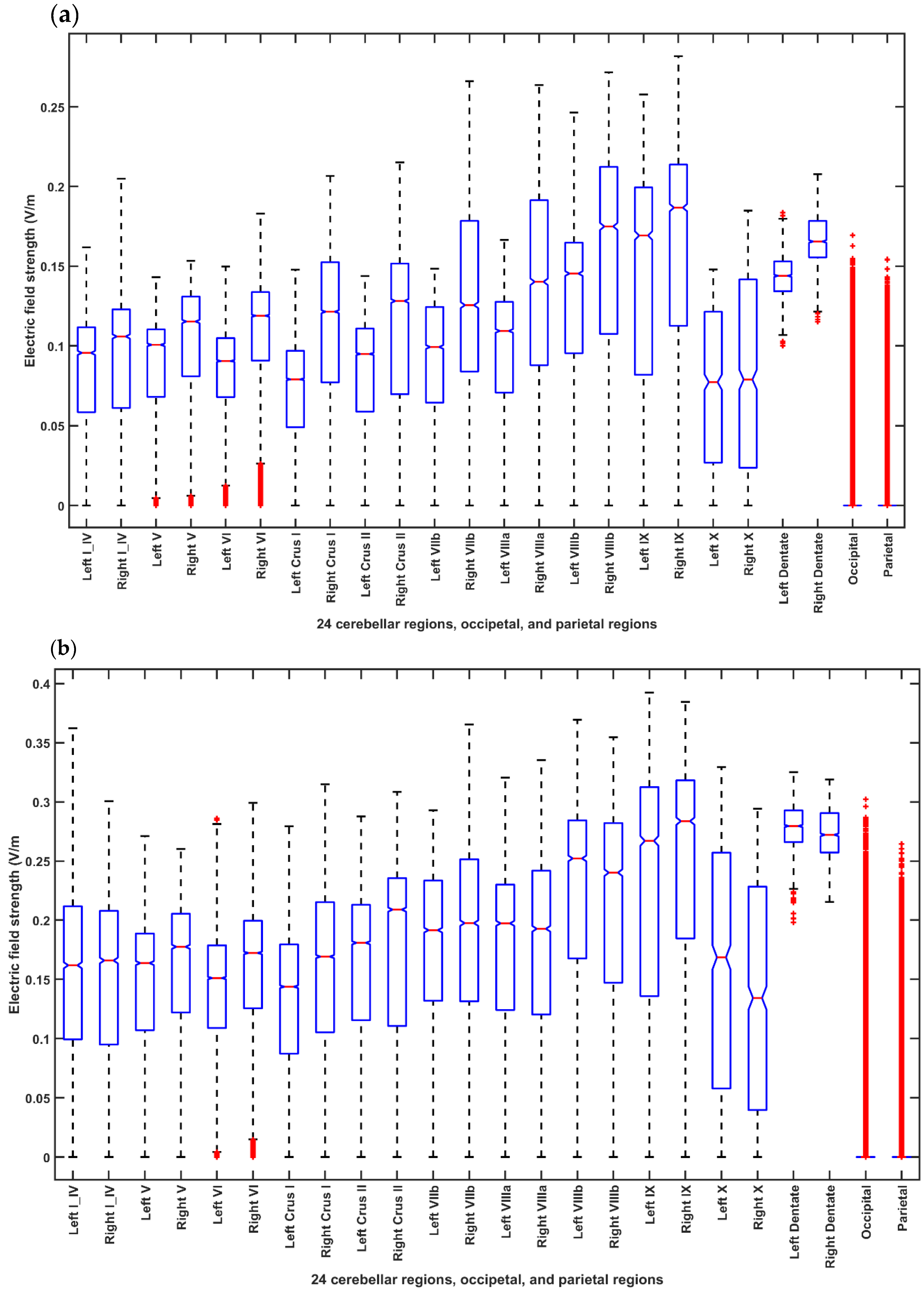
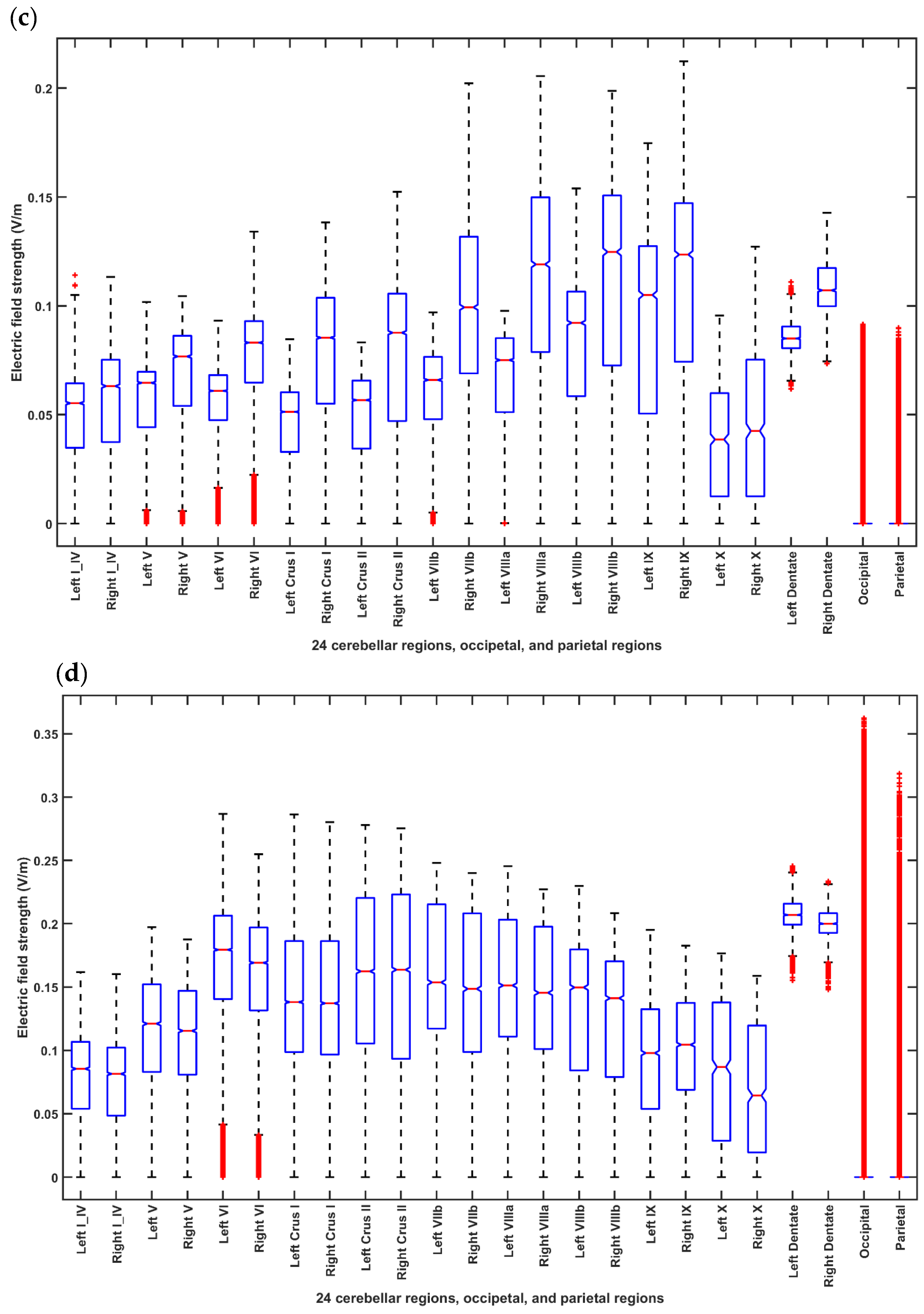
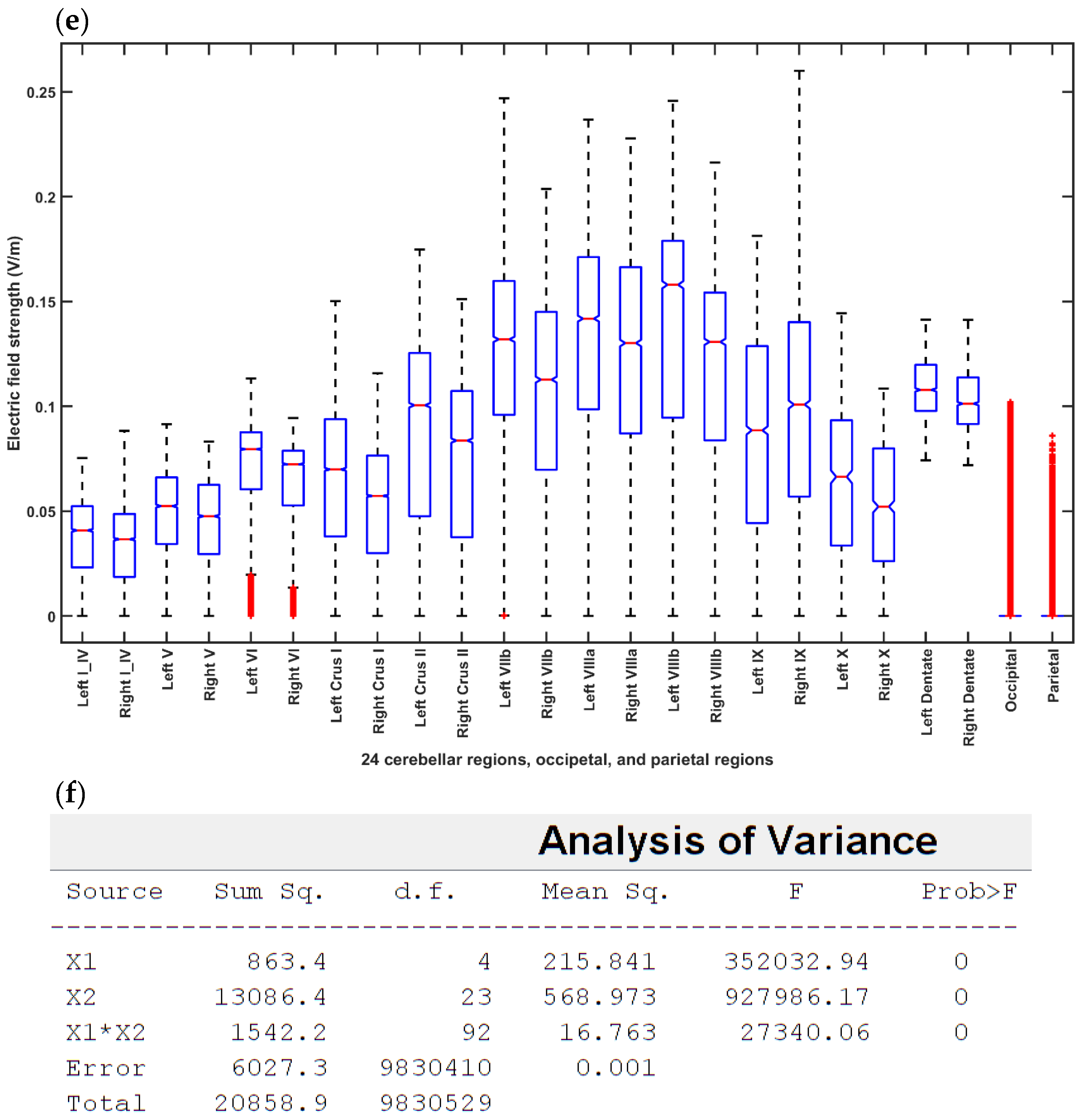
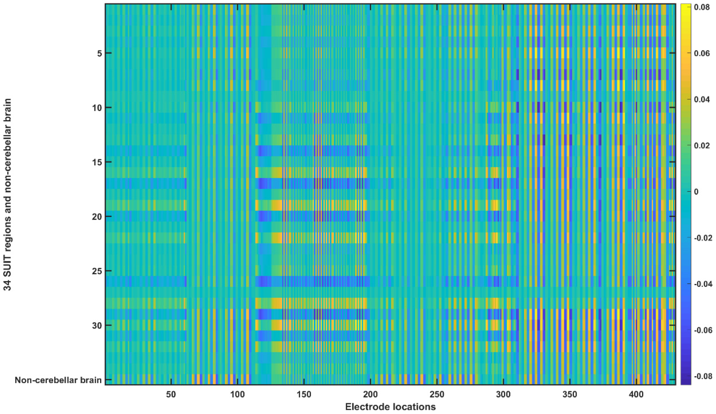
2.3.4. Assessing the Electric Field Distribution in the Cerebellar Lobules

FEA was performed with post-stroke MRIs (n = 10) using this reduced set of electrodes in the low-resource (point-of-care) setting constrained by a lack of computing power to generate the transfer matrices from the subject-specific post-stroke head models. Following FEA in ROAST, we used SUIT [52,53] to normalize the cerebellar electric field distribution. T1-weighted images were fitted to the SUIT template of the human cerebellum in SPM12 [40]. The cerebellar mask was visually checked in MRIcron (http://www.diedrichsenlab.org/imaging/propatlas.htm). Non-linear deformation was then applied to each electric field image obtained from ROAST. The volume of the cerebellar lobules, defined by the SUIT atlas [52], was used for the extraction of the lobular electric field distribution. We customized SUIT codes to assess the electric field distribution in the two dentate nuclei in addition to the 28 lobules. Here, vermis areas were excluded from further analysis. This reduced set of electrodes (see Figure 3) was faster to process using CVX (toolbox in MATLAB, Mathworks, MA, USA) with affine constraints [49] for ctDCS optimization. The resultant group-averaged bipolar montage (shown in Figure 2) was used on the 5 post-stroke participants who volunteered for ctDCS and FRT study (starred subjects in Table 1). So, we applied two bipolar montages limited to scalp overlying the cerebellum and the neck as listed below.
(1) Bipolar PO9h–PO10h montage for dentate nuclei: A 3.14 cm2 (1 cm radius) circular anode was placed at the contra-lesional side, and a 3.14 cm2 cathode was placed at the ipsilesional side for ctDCS with 2 mA direct current.
(2) Bipolar Exx7–Exx8 montage for bilateral leg lobules VII-IX: A 3.14 cm2 (1 cm radius) circular anode was placed at the contra-lesional side, and a 3.14 cm2 cathode was placed at the ipsilesional side for ctDCS with 2 mA direct current.
The bipolar electrode montage was modeled in ROAST at the given scalp locations to compute the electric field in the brain tissues [54]. In all simulations, the voxel size was considered as 1 mm3.

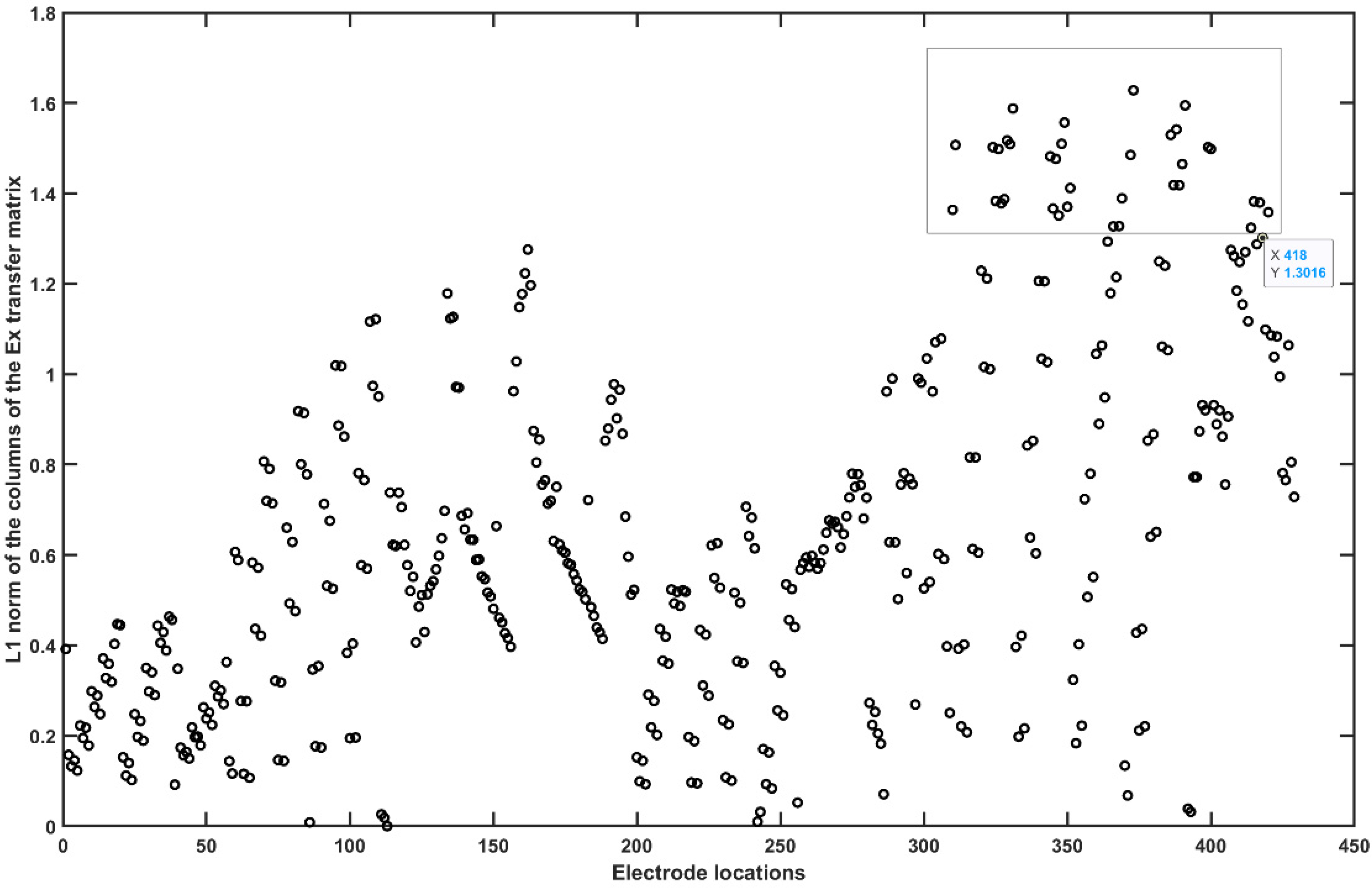
2.3.5. Assessing the Electric Field Distribution in the Occipital and Parietal Lobes

It was important to assess the electric field distribution in the cerebral volumes near the cerebellum for safety (avoid spillover to the lesioned brain). To evaluate the electric field distribution of the nearby occipital and parietal lobes, we created a mask for each lobe using MNI atlas in the FSL [55]. A code was scripted in MATLAB to isolate the electric field in the masked regions (occipital and parietal lobes) of the brain.

2.4. Statistical Analysis of the Electric Field Distribution in the Head Model of the 55 to 59 Years Old

The electric field was computed at all the voxels (voxel size 1 mm3) using ROAST [27] for the five montages (see Section 2.3.1). We analyzed the electric field distribution across lobules, dentate nuclei, and occipital and parietal lobes using two-way ANOVA (‘anovan′ in MATLAB) for the factors of interest – brain regions, montages, and their interactions (brain region*montage). In the Generalized Linear Model (GLM), the proportion of the total variability in the dependent variable that is accounted for by the variation in the independent variable found using the eta-squared effect size measure. Post-hoc multiple comparison tests were conducted using Bonferroni′s critical values.

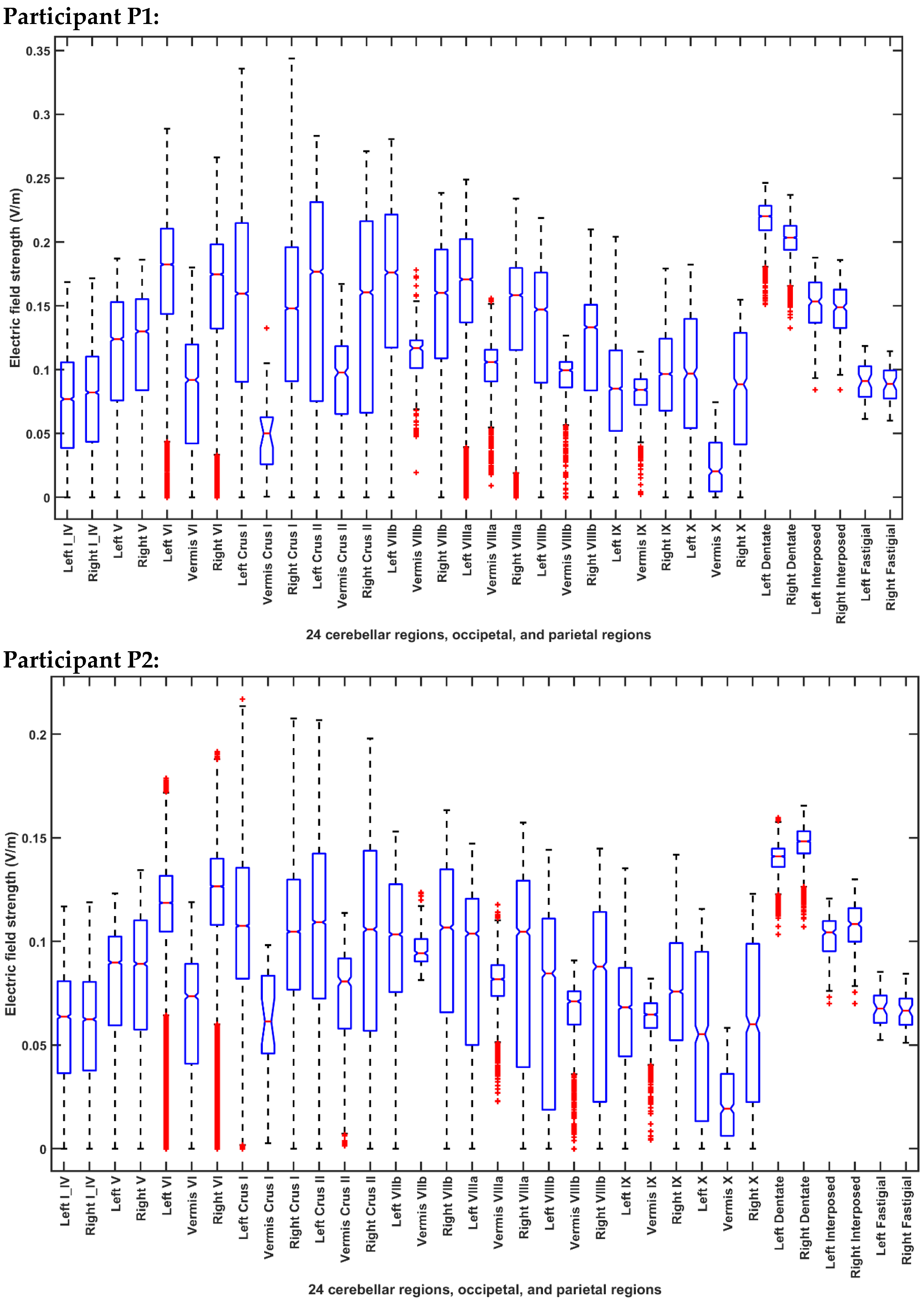
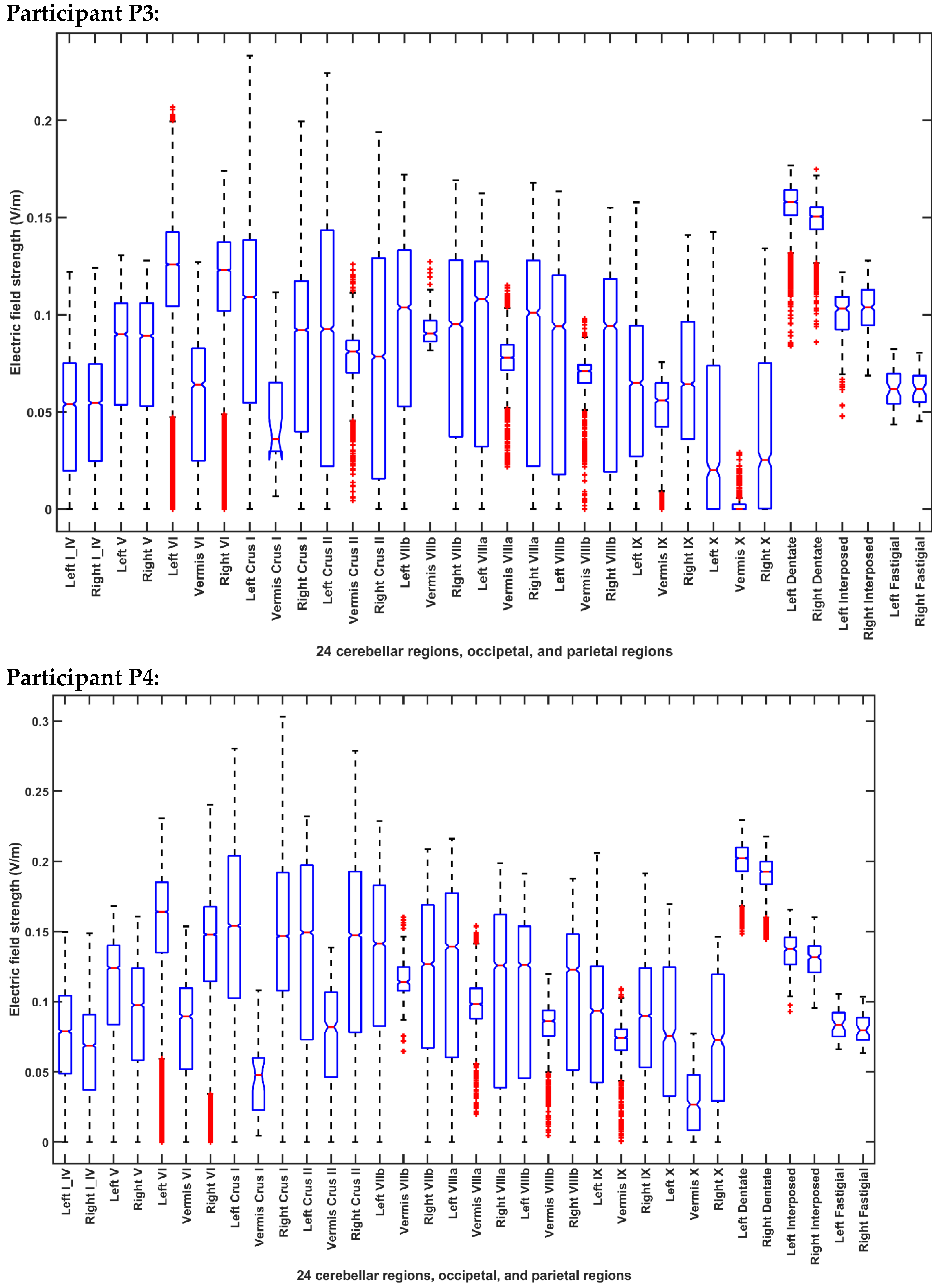
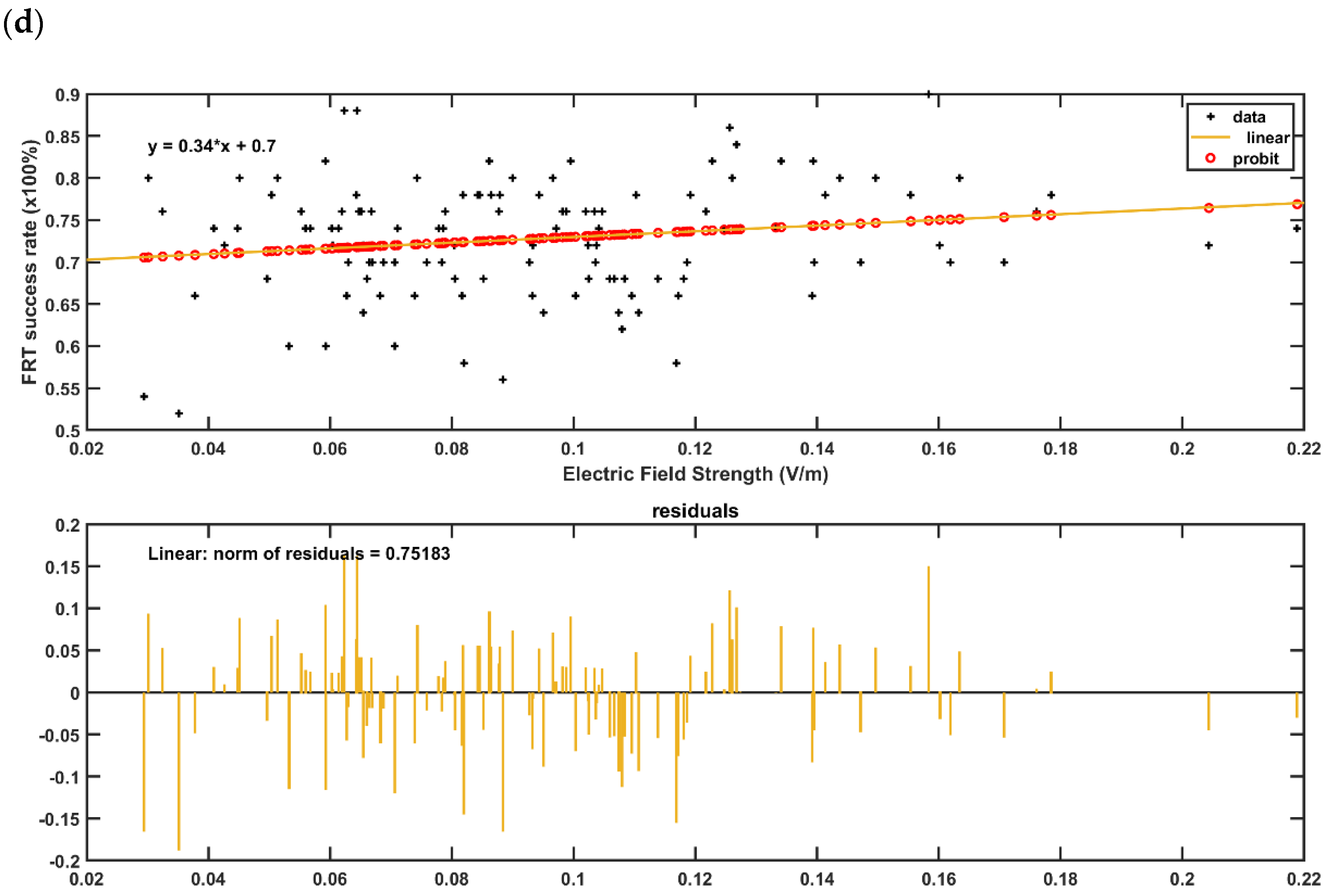
2.5. Regression Analysis of the Electric Field Distribution with the Behavioral Outcome in the Post-Stroke Subjects

Recent work shows that the cerebellum is organized in distinct functional subregions revealed by a multi-domain task battery (MDTB) based on Diedrichsen and Kriegeskorte [56,57] that provided a functional atlas. Therefore, ctDCS can have a multi-domain functional effect that can be elucidated with a multi-domain task battery (MDTB) [57] where a functional atlas can be used for the first optimization of ctDCS electrode montage. Here, the novel parcellation of the human cerebellum into functional regions using MTDB can be scaled as the spatial target for the electric field, E , where E vector can be constrained to be normal to the cerebellar surface in order to optimally target the Purkinje cells [7]. MDTB results also revealed a need for representational models that specify how the electric field, E , distribution due to ctDCS relates to motor responses or cognitive processes across MDTB, i.e., the distribution of activity profiles across experimental conditions. In the current study, we hypothesized that the electric field, E , distribution due to ctDCS has a linear relationship with the q behavioral outcome measures across p subjects (or, p trials of a single subject) represented by p × q behavioral outcome (continuous) matrix, B. Linear model, when applicable, needs to be appropriately regularized, which effectively imposes a prior on the activity profiles. Such a linear relationship can be captured by p × q × 3m regression matrix, A, i.e., B = A E + w , where w is the zero-mean normally distributed residuals not explained by the linear regression. Here, p × q behavioral outcome (continuous) matrix, B, can suffer from multicollinearity in a large multi-domain task battery so we may be able to reduce its dimension using principal component analysis and then the orthogonal dependent variables (i.e., uncorrelated functional profiles) can be individually fitted to the electric field, E , distribution as a predictor.
In our repeated-measure counter-balanced crossover study, we compared two bipolar montages across 5 post-stroke subjects (“one-size-fits-all”), bipolar PO9h–PO10h for dentate nuclei and bipolar Exx7–Exx8 for bilateral cerebellar leg lobules VII–IX, so the proportion of the total variability in the electric field, E , is postulated to be accounted for by the variation in the independent variables, brain regions, montages, stroke participants, and their interactions. This leads to a GLM using three-way ANOVA (‘anovan’ in MATLAB) for the factors of interest – brain regions, montages, stroke participants, and their interactions – based on their statistical significance. Here, the electric field, E , distribution is the dependent variable and different electric field, E , distribution can affect outcomes across MTDB [57]. Next, the outcomes, B, can be treated as a random variable and the goal is to predict, for each possible outcome, the probability of an electric field, E , distribution (or, related montages, I, if statistically significant from ANOVA) exhibiting that outcome. In the current study, we have one behavioral outcome, i.e., the number of successful target reaches (binomial distribution) during FRT trials, so q = 1. Here, the p × 1 behavioral outcome matrix, B, is the success rate at FRT trials post-intervention for the different electric field, E , distribution. This leads to a GLM for the dependent variable, B, using probit link (‘glmfit’ in MATLAB) for the predictor of interest (z-value of a normal distribution) – electric field, E , distribution. Baseline equivalence between the two groups was confirmed by the Wilcoxon rank-sum test (‘ranksum’ in Matlab).
We postulate that ctDCS optimization should be based on deficits in functional outcomes during quantitative multi-task evaluation due to cerebellar multiple functionalities [58] where ctDCS optimization can be based on mapping to universal cerebellar computations [58], e.g., relate to the executive cluster of the CCAS [59] in IMA. Importantly, King et al. recently showed that lobular boundaries commonly used to summarize functional data do not coincide with functional subdivisions [57]. Here, human dentate nuclei have also been found to be divided into three functional territories; default-mode, salience-motor, and visual brain networks [60]. Therefore, we propose a functional optimization of ctDCS for future clinical studies to maximize behavioral outcomes based on representational models. Here, the behavioral outcome (continuous) matrix, B, from a multi-domain task battery can be subjected to dimension reduction along the principal gradient, P, that can reveal mapping to universal cerebellar computations across multiple task domains. This may be related to cerebellar double motor representation (lobules I-VI and VIII), and its relationship with triple non-motor representation (lobules VI/Crus I, Crus II/VIIB, IX/X) where functional differences and similarities across these different representations were shown recently [61].
If the montages have a significant effect on, E , and the linear model holds, i.e., P = A E + w , then for the p × 1 principal gradient, P, the p × 3m regression matrix, A ^ = arg   min A ( ( P A E ) T C w 1 ( P A E ) ) , for a residual covariance matrix, Cw. Since, E = L I + e , so P = ALI + ( Ae + w ) , where the covariance of ( Ae + w ) is C w + AC e A T . Therefore, if A ^ is known from regression analysis (e.g., Figure 8 for our single outcome measure in this study) then the L2 regularized [48] optimal stimulation current sources for a given principal gradient, P, (e.g., cognitive or motor [62] as necessary for rehabilitation) can be found as I ^ = arg   min I ( ( P A ^ LI ) T ( C w + A ^ C e A ^ T ) 1 ( P A ^ LI ) + λ I 2 2 ) subjected to other constraints (see Section 2.3.2) under convex optimization [49]. Also, linear programming can maximize the p × 1 principal gradient, P, i.e., I ^ = arg   max I ( W T A ^ LI ) , where W R p is a vector of weights (unit vector in our case), under the following constraints used in this study:
Total anodal current is equal to the cathodal current;
i = 1 n I i = 0
Total anodal and cathodal current magnitude is below a set threshold of 4 mA for safety and comfort (i.e., maximum anodal or cathodal current is 2 mA);
j = 1 n | x j | 4
This can be solved using CVX toolbox in Matlab (Mathworks, Inc., MA, USA) for the stroke subjects based on a reduced transfer matrix, L ´ R 3 m × r , where I R r and r < n , i.e., I ^ = arg   max I ( W T A ^ L ´ I ) , after the forward selection approach to find r < n scalp stimulation current sources with the high norm of its corresponding L column (from the head model for the age group of 55–59 years).

3. Results

Figure 2 shows the head model from the MRI template of 55-59 years age-group which was used to generate the whole head transfer matrices (429 electrodes—See Appendix B: Table A2) to optimize the bipolar ctDCS montage. The reduced set of 87 electrode locations to optimize bipolar ctDCS montage were selected for high L1 norm of the columns of the transfer matrices related to cerebellar brain, namely (shown in Figure 3), “E145”, “E146”, “E156”, “E165”, “Ex1”, “Ex2”, “Ex3”, “Ex4”, “Ex5”, “Ex6”, “Ex7”, “Ex8”, “Exx10”, “Exx11”, “Exx12”, “Exx1”, “Exx2”, “Exx3”, “Exx4”, “Exx5”, “Exx6”, “Exx7”, “Exx8”, “Exx9”, “Exxz”, “Exz”, “I1h”, “I2h”, “Iz”, “NkB”, “NkL”, “NkR”, “O1”, “O1h”, “O2”, “O2h”, “OI1”, “OI1h”, “OI2”, “OI2h”, “OIz”, “Oz”, “P10”, “P10h”, “P7”, “P7h”, “P8”, “P8h”, “P9”, “P9h”, “PO10”, “PO10h”, “PO7”, “PO7h”, “PO8”, “PO8h”, “PO9”, “PO9h”, “POO10”, “POO10h”, “POO1h”, “POO2”, “POO2h”, “POO3h”, “POO8”, “POO9”, “POO9h”, “POOz”, “PPO10”, “PPO10h”, “PPO7”, “PPO7h”, “PPO8”, “PPO8h”, “PPO9”, “PPO9h”, “T5”, “T6”, “TPP10h”, “TPP7”, “TPP8”, “TPP8h”, “TPP9h”, “Z1”, “Z2”, “Z7”, “Z9”. In this study, we also wanted a low L1 norm of the columns of the transfer matrices (L1 norm < 0.01 selected—see Appendix C) for the non-cerebellar brain (i.e., row 35—see Appendix C) to avoid spillover to lesional cerebral areas in stroke subjects which limited the available electrode locations to “E145”, “E146”, “E156”, “E165”,”Ex1”, “Ex2”, “Ex3”, “Ex4”, “Ex6”, “Exx1”, “Exx2”, “Exx3”, “Exx4”, “Exx5”, “Exx6”, “Exx7”, “Exx8”, “Exxz”, “Exz”, “I1h”, “I2h”, “Iz”, “NkB”, “NkL”, “NkR”, “O2h”, “OI1h”, “OI2h”, “OIz”, “Oz”, “POO1h”, “POO2”, “POO2h”, “POOz”, “Z1”, “Z2”, “Z7”, “Z9”. This provided a reduced set of scalp electrode locations (primarily overlying the cerebellum) for stroke subjects.
The optimal bipolar montage found for the head model from the MRI template of 55-59 years age- group were Z7–POO2 for case 4 (optimization for dentate nuclei) and Exx5–Ex6 for case 5 (optimization for bilateral lobules VII–IX). For the post-stroke subjects undergoing ctDCS, we selected PO9h–PO10h for case 1 and Exx7–Exx8 for case 2 based on group-analysis of the subject-specific optimization since the lesional brain areas were primarily in the frontal lobe (occipital and parietal lobes were free from lesions) in the five post-stroke participants who volunteered for the ctDCS FRT study. Figure 4 shows the boxplot of the electric field (EF) strength for different ctDCS montages for the head model from the MRI template of 55-59 years age-group across 24 cerebellar regions, occipital and parietal lobes where Figure 4a shows the EF distribution for the Celnik montage, Figure 4b shows the EF distribution for the Manto montage, Figure 4c shows the EF distribution for the Extracephalic montage, Figure 4d shows the EF distribution for the PO9h–PO10h montage for case 1 (optimization for dentate nuclei), Figure 4e shows the EF distribution for the Exx7–Exx8 montage for case 2 (optimization for bilateral lobules VII–IX). Here, the electric field strength at the dentate nuclei was found to be high across all montages including the conventional Celnik and Manto ctDCS montages where the Manto montage from conventional ctDCS montages was found to be the best to stimulate the dentate nuclei in addition to the lower limb representations in the cerebellum. Also, the EF strength at the non-cerebellar occipital and parietal regions was found to be high (comparable to the Manto montage) for our PO9h–PO10h montage. However, the EF strength at the non-cerebellar occipital and parietal regions was found to be low (comparable to the Extracephalic montage) for the Exx7–Exx8 montage. Nevertheless, the median of the EF strength at the non-cerebellar occipital and parietal regions was low (<0.02 V/m), and most of the boxplot consisted of the outliers which are plotted individually using the + symbol. Here, Figure 4f shows two-way ANOVA results for the factors of interest–brain regions, montages, and their interactions (brain region*montage) which were all significant.
Figure 5 and Figure 6 present the boxplot of the electric field distribution for the 10 post-stroke patients for the PO9h–PO10h montage for case 1 (optimization for dentate nuclei) and for the Exx7–Exx8 montage for case 2 (optimization for bilateral lobules VII–IX) respectively. PO9h–PO10h montage for case 1 was optimized for the dentate nuclei which led to a higher electric field strength at the dentate nuclei as expected. However, PO9h–PO10h montage also led to an overall higher electric field strength at the bilateral leg lobules VII-IX when compared to the Exx7–Exx8 montage for the same stimulation current (2 mA). PO9h–PO10h montage also led to electric field spillover to the non-cerebellar occipital and parietal regions. Figure 7a shows three-way ANOVA results for the factors of interest–subjects, brain regions, montages, and their interactions which were all significant. Figure 7b shows the multiple comparisons of the population marginal means between the PO9h–PO10h montage and the Exx7–Exx8 montage which was found to be significantly (alpha = 0.05) different from each other. Figure 7c shows the multiple comparison test of the population marginal means of different brain regions (X2) where the dentate nuclei were exposed to a significantly (alpha = 0.05) higher electric field strength (>0.12 V/m) when compared to other brain regions across montages (X1) and subjects (X3). Figure 7d shows the multiple comparison test of the population marginal means of different subjects (X3) where the subjects P8-P10 were exposed to the significantly (alpha = 0.05) higher electric field strength when compared to other subjects across montages (X1) and brain regions (X2). Pre-intervention baseline equivalence of the FRT success rate (%) between the two repeated-measure counter-balanced crossover study groups was confirmed by the Wilcoxon rank-sum test that gave a p-value of 0.5216 so there was not enough evidence (5% significance level) to reject the null hypothesis of equal medians. The post-intervention FRT success rate (%) between the two repeated-measure counter-balanced crossover study groups gave a p-value of 4.6635 × e−5 so the null hypothesis of equal medians was rejected. Since the electric field, E , distribution, as well as the post-intervention FRT success rate (%), significantly varied so a GLM model (with probit link) was fitted to the independent variable, FRT success rate (%), as the p × 1 behavioral outcome matrix, B, from the FRT study. Figure 8 shows that a probit fit is comparable to a linear fit along with its linear regression residuals. The top panel of Figure 8 shows the GLM model (with probit link) results where the lobular maximum electric field strength is the predictor in Figure 8a and the lobular median electric field strength is the predictor in Figure 8b. FRT success rate (%) was found to be more sensitive to the lobular median electric field strength than the lobular maximum electric field strength, slope 0.17 versus 0.09. Also, the bottom panel of Figure 8 shows the GLM model (with probit link) results where the median electric field strength in the dentate nuclei is the predictor in the Figure 8c and the lower-limb area lobular median electric field strength is the predictor in the Figure 8d. Here, the FRT success rate (%) was found to be more sensitive to the lower-limb representations lobular median electric field strength than the dentate nuclei median electric field strength, slope 0.34 versus 0.27.

4. Discussion

In this pilot study on 5 stroke survivors, ctDCS of the dentate nuclei facilitated greater target reaches during FRT when compared to bilateral cerebellar lower-limb representations ctDCS. Inter-subject variability in the electric field strength at the cerebellum, as shown in Figure 7d, is expected due to the “one-size-fits-all” approach taken in this preliminary study. Nevertheless, Figure 8 shows that the FRT success rate (%) was positively related to the electric field strength at the cerebellum. Here, the FRT success rate (%) was found to be more sensitive to the lower-limb representations lobular median electric field strength than the dentate nuclei median electric field strength. Therefore, a higher electric field strength at the lower-limb representations of the cerebellum is postulated to be responsible for the improvements found during our VR-based based target reaching task where ctDCS montage for the dentate nuclei (PO9h–PO10h) resulted in a significantly (alpha = 0.05) higher electric field strength when compared to the ctDCS montage for the bilateral lower-limb representation of the cerebellum (Exx7–Exx8) for the same stimulation current (2 mA) as shown in the Figure 7b. Electric field strength due to ctDCS montage for the dentate nuclei (PO9h–PO10h) reached not only the dentate nuclei but also reached lobules Crus I and Crus II (see Figure 4d ,e), and even resulted in a higher electric field strength at the cerebellar lower-limb representations when compared to the ctDCS montage for the bilateral lower-limb representations of the cerebellum (Exx7–Exx8) for the same stimulation current (2 mA)—see Figure 4, Figure 5 and Figure 6. This is due to a different objective function used to optimize ctDCS montage for the dentate nuclei versus that for the bilateral lower-limb representations of the cerebellum. The optimal ctDCS montage for the bilateral lower-limb representations of the cerebellum aimed for the uniform electric field in the bilateral cerebellar lobules VII-IX whereas the optimal ctDCS montage for the dentate nuclei aimed for maximum electric field strength. Here, the ctDCS montage for the bilateral lower-limb representations of the cerebellum (Exx7–Exx8) will require a higher stimulation current to reach comparable electric field strength at the lower-limb representations of the cerebellum. Also, this pilot study was limited by “one-size-fits-all” ctDCS montage for the dentate nuclei as well as the bilateral lower-limb representations of the cerebellum. In future clinical studies, subject-specific ctDCS montages need to be tested for post-stroke balance training.
The proposed deep ctDCS targeting the dentate nuclei were found to be painless by all the 5 subjects where a weak direct current (= 2 mA) was delivered through a 2 cm diameter saline-soaked sponge electrode overlying the cerebellum. Skin irritation was found in one subject which can be due to a relatively high current density of 0.635 mA/cm2. Larger electrode size can ameliorate this issue in subjects with sensitive skin. Overall, bipolar bilateral ctDCS of the dentate nuclei performed better than the bipolar bilateral ctDCS of the cerebellar lower-limb representations for the same 2mA stimulation current where extensive reciprocal connectivity between the dentate nucleus and the wide swaths of cerebral cortex can affect motor as well as cognitive function [12]. Figure 4 shows that conventional ctDCS montages, e.g., Celnik, Manto, and Extracephalic, all affected the dentate nuclei so the functional effects due to these conventional ctDCS montages should be investigated not only based on its effects by polarizing Purkinje cells [13] but also based on its effects on the dentate nuclei. Also, the electric field effects of the Manto ctDCS montage were primarily focused on the cerebellar lower-limb representations which were found to be comparable to our ctDCS montage (Exx7–Exx8 montage)—see Figure 4b,e. We also found that electric field effects of our ctDCS montage for the dentate nuclei (PO9h–PO10h) reached lobules Crus I and Crus II (see Figure 4d) which can have beneficial cognitive effects by polarizing Purkinje cells. Nevertheless, the effectiveness of ctDCS of dentate nuclei needs to be tested as an adjuvant treatment to VR-based balance/weight-shifting training since the final goal is to improve functional outcomes. This pilot study was limited by a heterogeneous small sample size due to convenience sampling which consisted of 10 males within a large age range from 28 years to 59 years. Therefore, a larger clinical study is necessary to statistically confirm the effectiveness of ctDCS of the dentate nuclei with objective balance assessments.
During balance rehabilitation, an objective assessment of the balance and posture during functional reach tasks (FRT) or cued weight-shifting will require optical motion analysis technology that can provide a sensitive measure. However, marker-based systems (e.g., VICON, UK) are too expensive for monitoring in a community setting not only in developing countries but also in developed countries including the USA. Therefore, we developed marker-less time-of-flight systems [16,26,63,64], including the low-cost (<$150) Microsoft Kinect sensor (developed for video gaming), that are increasingly used for motion capture due to its lower costs [65]. Also, postural sway based on the center of pressure (CoP) is important for balance assessment; and the Wii Balance Board (WiiBB) has demonstrated good test-retest reliability (ICC = 0.66–0.94) and construct validity when benchmarked against laboratory-grade force platforms (ICC = 0.77–0.89) [66]. In principal accordance, we used low-cost (<$150) WiiBB for standing balance tests where cursor tracking in the virtual reality (VR) using CoP has been implemented and tested for usability [23]. This HMI has also been tested under an operant conditioning paradigm for balance training [67] where the cursor (a VR object) controller is designed such that it is less challenging to control using paretic leg to reach the cued VR targets, and this innovative approach can ameliorate learned non-use of the paretic leg by encouraging its increased use during adaptive VR-based weight-shifting tasks [67]. We postulate that operant conditioning can lead to learned internal representations and response to stimuli that can be facilitated with adjuvant treatment with ctDCS [68,69]. Here, VR-environment for FRT is postulated to be motivating thereby improving the therapy effects (Gil-Gómez et al., 2011). Indeed, systematic review and meta-analysis based on forty-three randomized controlled trials have shown that balance capacities can be improved by well-targeted exercise therapy programs, specifically, balance and/or weight-shifting training, in the chronic phase after stroke [70]. Furthermore, another systematic review and meta-analysis based on literature searches in databases including PubMed, Embase, MEDLINE, and Cochrane Library by de Rooij et al. [71] showed that VR training is more effective than balance training without VR for improving balance ability in patients with stroke. Also, a systematic review on feasibility and effectiveness based on literature searches in five databases including PubMed and the Cochrane Library [72] showed that VR can increase motivation allowing longer and more training sessions in community-dwelling stroke survivors. Nevertheless, there exists very little evidence about interventions other than exercises, e.g., ctDCS, that can improve post-stroke standing balance function [73].
To investigate post-stroke standing balance function, CoP trajectories during cued weight shifts in different directions during FRT [23] can elucidate ideomotor apraxia (IMA) found in our subjects, which may contribute to patients overall day-to-day motor disability [74]. IMA of lower limbs has rarely been investigated systematically [75] even though it has high relevance for maintaining independence in daily life activities [76]. Furthermore, IMA is one the earliest disturbances in Alzheimer′s disease [77] where disruption of the cerebrocerebellar network has been hypothesized based on the executive cluster of the cerebellar cognitive affective syndrome (CCAS) [59]. We recently presented ctDCS for healthy aging [78] where bipolar bilateral ctDCS can be a low-cost intervention that needs to be validated using a prospective, randomized, placebo-controlled, double-blinded, clinical study. Also, according to the majority of studies in the literature, limb apraxia in right-handed stroke patients is a disorder that typically occurs in 30–50% of the patients with left hemisphere damage and 0 to 30% in patients with right hemisphere damage [76]. Here, post-stroke IMA patients with left posterior parietal and/or premotor cortex lesions but intact cerebellum can be suitable for ctDCS. Therefore, we are investigating the feasibility of our mobile VR-based balance training in conjunction with bilateral ctDCS in the right lower limb post-stroke IMA with left hemisphere damage [75]. IMA is also an area of scientific significance for our operant conditioning approach to balance training [67] where one can learn how the normal human praxis system improves in IMA during adaptive balance training [67]. This is postulated due to IMA’s cerebellar component related to cardinal motor deficits which are thought to arise from damage to the cerebrocerebellar network communicating internal representations for actions. Here, an early operant conditioning approach to balance training [67] in a community setting after stroke may be crucial for recovery through learning and experience [79]. Recovery through balance training [67] is crucial since falls are more likely in the apraxias [80], and the severity of apraxia predicts the rehabilitation success for patients with hemiplegia [76]. In principal accordance, an augmented mobile VR interface can allow remote delivery of new VR balance training games to keep the motivation for home-based intervention. To address usability issues with individualized ctDCS montage, we have developed an innovative low-cost washable neoprene cap with subject-specific stitched saline-soaked electrodes that can be worn during balance training [20]. Such a home-based upper-limb training approach has also been proposed by de Winckel and colleagues [22], however, our approach is novel for lower limb balance training.
Our optimization approach for a minimal set of electrodes for home-based tDCS is based on an open-source computational pipeline [7] that aimed to keep the bilateral ctDCS electric field limited to the cerebellum and away from the cerebral areas that were lesioned in our stroke subjects. Here, first, a reduced set of electrodes (see Figure 3) relevant for focal stimulation of the cerebellum were identified in the stroke subjects for the optimization of a “one-size-fits-all” bipolar electrode montage for ctDCS, as discussed in the Methods section. This two-step process to identify a “one-size-fits-all” bipolar electrode montage to target cerebellar lobules and nuclei is postulated to be more practical in low-resource home-based or community-based settings constrained by a lack of computing power and high-quality neuroimaging data. However, our innovation in optimizing the lobular electric field for patient-relevant functional outcome and neuroplastic effects in stroke survivors is also important for patient-specific dosing based on MRI data that may reduce inter-individual variability [81]. Here, optimization based on the relevant component of the electric field [81] needs to be verified for different cerebellar lobular targets, including the molecular layer, the granule cell layer and the Purkinje cell layer, since different ctDCS electrode montages can affect different parts of the cerebellum (and cerebellar circuit) [7] leading to different functional outcomes and neuroplastic effects. For example, anodal ctDCS using Celnik montage [13] affected the adaptation rate of spatial but not temporal elements of walking where the spatial adaptation was postulated to be related to pontocerebellum stimulation [10]. Our open-source computational modeling pipeline [7] confirmed that the magnitude of the electric field for Celnik montage [13] primarily targeted the pontocerebellum as postulated in the experimental paper by Jayaram et al. [10]. The innovation lies not only in the ability to optimize the lobular electric field in the cerebellum [7] but also in the augmented approach to address functional heterogeneity [58] based on the outcomes from a task battery. Here, post-stroke deficits can cover multiple task domains that can be elucidated with multi-domain behavioral experiments (e.g., FRT balance function, hand function, gait function, cognitive function) to develop an appropriate objective function for ctDCS optimization that addresses cerebellar multiple functionalities [58]. Here, optimization of the lobular electric field in the cerebellum [7] is challenging without subject-specific neuroimaging guided head modeling due to the extreme folding of the cerebellar cortex. We also postulate for future studies that ctDCS optimization needs to be based on the mapping to universal cerebellar computations (e.g., comparator function) [58] that can ameliorate deficits in multiple task domains [58].
Neurorehabilitation service delivery at homes and in the community settings can incorporate mobile-health based approaches to low-cost neurotechnologies that are tailored to an individual health condition as identified based on WHO International Classification of Functioning (ICF) [82]. Here, functional optimization of ctDCS will require a large patient outcome dataset possible using big data mobile-health (mHealth) approaches that also requires sustainable and multi-professional rehabilitation systems, including the provision of services to the rural population. This was investigated by a randomized controlled trial on family-led rehabilitation after stroke in India (ATTEND) [83]. In the ATTEND trial, regular stroke rehabilitation services provided by family caregivers were found not effective even after structured training including information provision, joint goal setting, carer training, and task-specific training [83]. ATTEND trial suggested investigation of the effects of task shifting to health-care assistants or team-based community care that necessitated telerehabilitation strategies due to the scarcity of trained professionals in India. Furthermore, telestroke model in India for thrombolysis in acute ischemic stroke showed that smartphone-based telestroke services may be a much cheaper alternative to video-conferencing-based telestroke services and are more portable with less technical glitches [84]. India is ripe for the assessment of the feasibility and usability of telemedicine approaches not only in acute stroke [84] but also in chronic stroke. Tele-rehabilitation is also justified since functional improvements have been found to be equal for telerehabilitation and virtual reality (VR)-based training when compared to a similar intervention with therapist-supervision in the clinic [72]. Therefore, we propose testing of the effectiveness of a low-cost neurotechnology platform [23] for remote (smartphone-based) patient care and monitoring through the hub and spoke model (HSM) of telemedicine that is not only necessary to create a large patient outcome dataset but is also crucial to meet the growing needs of stroke survivors in India [85,86]. In the HSM of neurorehabilitation, the service delivery assets into a network consist of an anchor establishment (hub) which will offer a full array of services, complemented by secondary community-based establishments (spokes) that can offer local neurorehabilitation service arrays, routing patients needing more intensive services to the hub for treatment. Here, the feasibility of an online assessment document called ‘Rehabilitation Problem-Solving Form’ (RPS-Form) [87] was shown by us in a preliminary study in India to monitor patient’s response to a short-duration moderate-intensity neurostimulation therapy by assessing all the ICF components. Here, our innovative online RPS-Form captures patients’ perspective that has been shown in our preliminary study [87] to facilitate communications between the patient (at the spoke in HSM) and his/her multi-disciplinary rehabilitation team (at the hub in HSM) consisting of physiotherapists, occupational therapists, medical doctors, and rehabilitation engineers. Such multi-session neurotechnology intervention may be necessary for a community setting where post-stroke remote tDCS plus target tracking training has been shown feasible and usable for upper limb [22], however, the feasibility of remote delivery of ctDCS in conjunction with mobile VR-based balance training in a low resource community setting is unknown. Here, the feasibility and usability testing of remote delivery of ctDCS are crucial since usability issues could lead to user error that has the potential to compromise patient safety and negatively impact the quality of therapy and outcomes.

5. Conclusions

We developed and evaluated a rational approach to optimize deep ctDCS of the dentate nuclei and lower limb representations in the cerebellum for post-stroke balance rehabilitation. Our pilot study presented promising results on the beneficial effects of deep ctDCS on functional reach during a standing balance task in chronic stroke survivors. However, our clinical study in a low-resoure setting was limited by “one-size-fits-all” bipolar ctDCS montage as well as a small sample size.

Author Contributions

Study conceptualization and design, A.D. (Anirban Dutta); methodology, Z.R., A.D. (Anirban Dutta) and U.L.; software, Z.R., D.S.; validation, A.D. (Anirban Dutta), U.L., and M.V.P.S.; formal analysis, A.D. (Anirban Dutta) and Z.R.; investigation, Z.R., D.S., A.D. (Adyasha Dash) and S.K.; resources, A.D. (Anirban Dutta), U.L., and M.V.P.S.; data curation, Z.R., D.S. and S.K.; writing—original draft preparation, A.D. (Anirban Dutta) and Z.R.; writing—review and editing, A.D. (Anirban Dutta), U.L., and M.V.P.S.; visualization, Z.R.; supervision, A.D. (Anirban Dutta), U.L., and M.V.P.S.; project administration, A.D. (Anirban Dutta), U.L., and M.V.P.S.; funding acquisition, A.D. (Anirban Dutta), U.L., and M.V.P.S. All authors have read and agreed to the published version of the manuscript.

Funding

This research was funded by the Indian Ministry of Human Resource Development (MHRD)′s Scheme for Promotion of Academic and Research Collaboration (SPARC), grant number 2018−2019/P721/SL, and Indian Department of Health Research, Project Code No. N1761.

Acknowledgments

Authors would like to acknowledge the technical support from Brandon Ruszala for the development of the CLOS pipeline. Initial technology development and experimental validation of the HMI by Deepesh Kumar during his doctoral research is also acknowledged by the authors. Authors also acknowledge the initial funding (2014−2017) by the Department of Science and Technology (DST), India and Institut National de Recherche en Informatique et en Automatique (Inria), France—https://team.inria.fr/nphys4nrehab/.

Conflicts of Interest

The authors declare no conflict of interest.

Appendix A

Table A1. The 34 SUIT labels are.
1Left I_IV10Right Crus I19Right VIIIa28Right X
2Right I_IV11Left Crus II20Left VIIIb29Left Dentate
3Left V12Vermis Crus II21Vermis VIIIb30Right Dentate
4Right V13Right Crus II22Right VIIIb31Left Interposed
5Left VI14Left VIIb23Left IX32Right Interposed
6Vermis VI15Vermis VIIb24Vermis IX33Left Fastigial
7Right VI16Right VIIb25Right IX34Right Fastigial
8Left Crus I17Left VIIIa26Left X
9Vermis Crus I18Vermis VIIIa27Vermis X

Appendix B

Table A2. 429 electrode locations (including fiducials and reference electrodes) with the X, Y, Z for 55–59 years head model are.
No.LocationxyzNo.Locationxyz
1Fp1−22.559282.9048813.87207216P5h−62.6435−55.41748.50705
2Fpz3.84229687.0361617.49313217P3h−44.5991−62.238271.54874
3Fp228.5267883.5557813.67529218P1h−15.6894−68.094783.5882
4AF7−41.997671.2404812.12234219P2h19.79522−68.73883.61536
5AF5−34.664775.1093825.48365220P4h49.80881−62.995571.23532
6AF3-25.390478.6030535.73096221P6h67.89475-54.850247.65088
7AF1-11.94179.8082443.49709222P8h73.34005−48.408922.94698
8AFz2.70088180.8320945.4243223P10h74.35319−44.3501−5.70373
9AF218.3883480.301643.27522224PO9h−55.5975−70.1245−6.82361
10AF432.6685178.8377135.49923225PO7h−54.5191−76.033519.40764
11AF641.6306375.4140525.66882226PO5h−45.1531−82.196735.4382
12AF847.4969772.0057813.61991227PO3h−29.3346−88.084447.25826
13F9−55.9450.26538−18.4116228PO1h−8.08273−90.920553.45393
14F7−56.172453.0370111.21066229PO2h13.28204−91.06852.90984
15F5−50.874456.2102531.86567230PO4h32.52896−88.408447.14226
16F3−39.095259.7721850.02259231PO6h50.25244−81.43135.07223
17F1−20.103363.80363.89388232PO8h59.58925−74.912819.71736
18Fz2.9971265.0825769.42619233PO10h61.64832−69.6594−5.77207
19F227.3684263.4777164.33418234O1h−16.0684−100.44816.96381
20F445.6599560.4467150.90544235O2h20.76301−100.28515.9655
21F657.0342157.1277533.22234236I1h−11.759−96.2474−22.6608
22F862.1844953.9264712.13087237I2h16.51372−96.2668−21.869
23F1061.5201751.90641−17.3684238AFp7−32.066478.358713.15924
24FT9−66.237132.61463−20.9561239AFp5−25.927580.7501221.30455
25FT7−65.319431.5080511.14653240AFp3−19.288482.7390828.30598
26FC5−62.089932.1592937.65389241AFp1−8.2879284.6865531.39793
27FC3−49.372733.471561.182242AFpz3.52684585.0081832.90711
28FC1−26.79137.6875380.24023243AFp214.765284.9275131.13003
29FCz4.25383338.9196987.41366244AFp424.7335583.5539128.15581
30FC233.3150737.8310380.37218245AFp633.5251180.7592522.74153
31FC456.883233.7827861.13577246AFp837.8140279.4077212.13282
32FC669.4199831.8848337.35075247AFF9−48.163662.60542−15.9273
33FT872.1251131.0966411.29649248AFF7−49.545263.0608911.20612
34FT1072.2873631.96451−21.5403249AFF5−43.424766.7226628.63601
35T9−68.49988.249681−22.4725250AFF3−32.721169.9212443.53524
36T7−71.38535.0569811.08433251AFF1−16.686672.8226153.58292
37C5−69.2293.88409542.42783252AFFz4.28883274.7117357.53587
38C3−57.7473.71783167.76955253AFF222.8442373.1677954.42189
39C1−31.58174.96747789.48766254AFF438.4879171.4105543.94503
40Cz3.4564955.32964299.52775255AFF650.0304367.0297329.6401
41C238.092385.8229188.99616256AFF855.6507763.688711.91936
42C464.267014.36962167.62971257AFF1054.2640662.65546−16.8431
43C675.434026.50590942.33944258FFT9−62.32341.66684−20.9349
44T877.386026.5302289.717833259FFT7−61.323442.5876110.88625
45T1074.502887.909821−22.3627260FFC5−57.024744.44134.49869
46TP7−73.5016−21.514510.67297261FFC3−44.697646.6125156.76297
47CP5−71.524−24.361442.38637262FFC1−24.290851.5522572.34157
48CP3−61.6892−27.372669.56094263FFCz3.46513354.2273579.14475
49CP1−33.5793−28.531492.61813264FFC231.0000151.9175872.89468
50CPz3.611006−29.6046102.548265FFC451.296248.0126157.39484
51CP240.46755−28.572392.68565266FFC664.1818544.1112835.40215
52CP467.15958−26.254970.12574267FFT868.2642.4424210.99613
53CP677.5511−23.114340.75406268FFT1067.7798642.6417−21.5682
54TP879.52268−20.99959.849888269FTT9−68.267319.54876−20.5511
55P9−67.2474−45.3603−21.1713270FTT7−68.489519.3065410.96369
56P7−68.778−46.065311.4691271FCC5−66.150819.1065640.53259
57P5−66.2887−52.51336.08666272FCC3−54.275617.8866264.73584
58P3−54.9608−59.644260.7231273FCC1−29.382120.9585186.31815
59P1−29.4783−66.377279.33228274FCCz3.95881822.0033294.121
60Pz1.16076−67.046186.85532275FCC235.5261222.5981685.42201
61P235.68975−66.379579.29573276FCC460.7579719.8873564.52368
62P460.31538−59.888559.73956277FCC672.3289621.0687440.94543
63P671.43842−51.495435.46394278FTT875.1599819.0723411.70313
64P874.42983−46.159810.89193279FTT1074.1830119.9038−19.5862
65P1073.05866−44.5554−22.0247280TTP7−73.2764−8.5987711.85397
66PO9−55.4014−66.2734−22.0704281CCP5−71.2532−9.3382642.32324
67PO7−57.4879−72.080411.77603282CCP3−61.0012−11.126768.91452
68PO5−50.2619−79.283227.65109283CCP1−33.6162−11.710391.75061
69PO3−38.3293−85.410141.33633284CCPz3.522455−12.3699102.5344
70PO1−18.2358−90.25350.93382285CCP240.14838−11.174692.32234
71POz3.252028−91.05754.66248286CCP466.77457−10.846970.0064
72PO224.01926−90.005750.48114287CCP677.44537−8.4946541.47523
73PO442.66196−85.439140.63985288TTP879.36731−7.5753711.90171
74PO655.28989−78.390127.5132289TPP9−69.0679−26.4722−22.8065
75PO862.37442−71.684711.74387290TPP7−72.1635−32.964810.49897
76PO1060.72315−67.1283−20.8686291CPP5−70.2081−37.213939.19454
77O1−32.7194−94.012114.27106292CPP3−60.0331−43.435465.72448
78Oz3.040962−102.26117.13088293CPP1−33.7106−48.891588.78305
79O238.5953−93.105413.28896294CPPz3.471033−50.157896.55543
80O9−31.4911−90.3528−22.2667295CPP241.27761−47.540188.19879
81O1035.9837−91.066−21.1492296CPP465.71957−43.065765.24334
82I1−31.4911−90.3528−22.2667297CPP675.38837−37.513739.31531
83I235.9837−91.066−21.1492298TPP878.0984−32.642111.23656
84AFp9h−33.493179.64136−1.93019299TPP1077.33778−26.388−23.5285
85AFp7h−29.07579.4813117.76607300PPO9−62.4592−53.9455−21.5535
86AFp5h−22.349982.0106925.16756301PPO7−64.3126−60.004311.86185
87AFp3h−14.440683.7433530.16004302PPO5−60.4425−66.135931.64876
88AFp1h−2.9014885.0402231.85801303PPO3−47.0598−74.488551.85476
89AFp2h9.67553585.0908432.41395304PPO1−25.6341−79.834165.64269
90AFp4h19.428884.6137429.56817305PPOz2.544747−82.108469.75008
91AFp6h28.5492182.6992224.88188306PPO230.92945−80.004165.53837
92AFp8h34.6798280.5353217.90698307PPO452.82137−73.594451.12067
93AFp10h39.6157279.72829−3.10175308PPO665.23055−65.126231.95901
94AFF9h−50.373165.10702−5.09855309PPO869.65572−58.32510.88854
95AFF7h−47.219764.6423921.10871310PPO1067.54266−54.4292−22.6903
96AFF5h−38.065969.2064335.60582311POO9−46.5394−78.0818−22.3323
97AFF3h−25.671371.193149.07541312POO7−47.1039−83.409113.77876
98AFF1h−6.3259173.7285557.30378313POO5−38.0156−90.04522.25939
99AFF2h13.2815674.0215557.3758314POO3−26.5354−95.008730.24876
100AFF4h32.1430172.0044449.46066315POO1−11.3729−97.507135.97657
101AFF6h45.6277268.7217137.0618316POOz1.421684−98.170336.50932
102AFF8h52.9666866.0757920.63462317POO218.62236−97.262834.81373
103AFF10h56.2092665.41907−5.3522318POO433.08083−93.882529.92061
104FFT9h−62.208242.18876−7.02438319POO643.59314−89.064322.69428
105FFT7h−60.20843.7107222.80203320POO852.61583−82.925813.22738
106FFC5h−52.100845.2152746.08334321POO1052.20508−78.4769−21.0116
107FFC3h−35.246349.0172665.63649322OI1−33.6804−92.1769−4.83753
108FFC1h−10.051951.6720578.71602323OIz2.777775−101.21−5.77148
109FFC2h16.6363752.1478378.93129324OI238.28328−92.2741−4.78841
110FFC4h41.6530450.3555366.03575325T3−71.38535.0569811.08433
111FFC6h58.8519546.5283446.21732326T5−68.778−46.065311.4691
112FFT8h67.1180342.8977424.38205327T477.386026.5302289.717833
113FFT10h68.2358442.95902−6.70591328T674.42983−46.159810.89193
114FTT9h−68.314320.6105−6.39526329Exz3.413347−94.1549−34.1897
115FTT7h−68.13419.940427.09219330Ex1−8.96197−94.2189−34.75
116FCC5h−62.230317.1879652.15804331Ex213.74652−94.1877−33.868
117FCC3h−42.151319.7522677.24973332Ex3−36.2817−82.5359−38.5457
118FCC1h−12.903622.051191.96693333Ex443.2247−80.4344−40.514
119FCC2h19.4188722.724391.5395334Ex5−45.9755−71.6576−39.8934
120FCC4h49.6914320.5515876.14634335Ex651.25343−72.2088−40.2305
121FCC6h68.290118.717253.31686336Ex7−53.701−60.5663−40.0393
122FTT8h75.1045319.1103625.89622337Ex860.58237−59.2705−39.1244
123FTT10h74.329621.48304−7.01454338Ex9−59.7161−48.2031−38.4779
124TTP7h−73.2487−9.1911126.35322339Ex1065.82136−47.2179−39.1501
125CCP5h−68.0965−11.918756.38265340Ex11−61.9403−42.6414−39.7219
126CCP3h−49.0741−11.607482.11982341Ex1268.00566−42.5266−39.2374
127CCP1h−15.7263−11.678199.48219342Ex13−65.1545−22.0944−31.4051
128CCP2h21.99551−11.296699.28143343Ex1469.53552−21.2467−32.9172
129CCP4h55.17046−11.688182.76363344Ex19−67.12888.122559−35.3273
130CCP6h74.18729−8.8951255.26226345Ex2072.71488.95946−35.0052
131TTP8h79.55205−7.0323725.88526346Ex21−65.735919.52943−34.2457
132TPP9h−73.1609−31.863−6.42023347Ex2271.6770720.64119−34.9331
133TPP7h−71.2541−35.664325.71736348Ex23−64.418730.91435−34.9063
134CPP5h−66.9441−40.784752.23498349Ex2470.6926130.84808−34.6901
135CPP3h−48.5238−46.019378.62906350Ex25−61.079441.18943−35.0183
136CPP1h−16.212−48.347395.56354351Ex2666.7376441.93864−34.4454
137CPP2h22.19478−48.915795.74229352Ex27−54.562351.50744−34.1932
138CPP4h54.62639−44.867878.57848353Ex2860.4430751.08272−33.6067
139CPP6h72.4343−40.448651.81738354Ex29−46.659758.25651−33.7596
140TPP8h77.38898−35.524824.96803355Ex3052.0083759.01769−33.3612
141TPP10h78.72811−31.5109−7.08444356Ex31−37.356664.40849−32.5878
142PPO9h−63.5017−57.5402−6.52086357Ex3242.7980964.87608−33.3054
143PPO7h−63.334−62.143522.93271358Ex33−27.809869.11741−31.0611
144PPO5h−54.6809−70.914742.44857359Ex3434.6023269.6494−30.5847
145PPO3h−37.0488−78.176759.33378360Exxz2.600347−88.223−53.4067
146PPO1h−11.9075−81.224569.38043361Exx1−14.7184−87.6082−53.7016
147PPO2h17.13343−81.293969.21624362Exx212.11622−88.1398−53.8715
148PPO4h43.56473−76.698359.87423363Exx3−39.6464−73.0199−51.5006
149PPO6h60.5297−69.120142.01922364Exx444.51721−73.1659−52.6129
150PPO8h67.73132−61.857121.41818365Exx5−49.3719−59.3122−53.2278
151PPO10h69.40595−56.9527−5.5405366Exx654.64212−60.8592−52.4478
152POO9h−46.5702−81.4362−6.27118367Exx7−54.6454−44.98−54.0367
153POO7h−42.5362−87.141917.76792368Exx859.84738−49.264−52.8618
154POO5h−32.906−92.456626.75433369Exx9−56.4254−37.1207−53.3956
155POO3h−18.1407−97.071832.9983370Exx1063.56102−35.4075−53.3598
156POO1h−4.35032−98.197436.47809371Exx11−57.4456−29.9627−53.944
157POO2h10.44098−98.173535.64018372Exx1264.68636−31.6225−53.0232
158POO4h24.9554−96.037133.98659373Exx13−59.97−21.5577−55.1901
159POO6h39.33543−91.276326.13067374Exx1466.54841−22.0255−55.3961
160POO8h48.66409−85.852117.3463375Exx15−62.8827−8.8041−51.3662
161POO10h51.90488−81.7238−3.61663376Exx1669.73143−8.80946−51.6004
162OI1h−16.2967−99.2963−5.70751377Exx19−62.684310.32494−49.7987
163OI2h19.77029−99.3035−5.48463378Exx2068.7989810.01529−50.2973
164Fp1h−11.06985.7890616.19175379Exx21−62.726618.11554−47.6526
165Fp2h17.4042586.0006816.62331380Exx2268.6875818.27113−48.8729
166AF9h−43.129973.41663−3.09828381Exx23−62.651226.49811−46.3039
167AF7h−38.028373.3938920.26724382Exx2468.6565928.04243−48.9772
168AF5h−31.28976.6660430.64554383Exx25−60.779438.99−46.6925
169AF3h−19.729879.6774638.74554384Exx2665.7175441.25271−46.1681
170AF1h−5.3416680.6579744.42367385Exx27−54.892650.79774−45.9224
171AF2h11.6248680.6636344.63826386Exx2861.0932749.51846−47.248
172AF4h25.9284779.9629839.45565387Exx29−46.668460.09819−43.8871
173AF6h37.1020977.5342931.11362388Exx3053.1561859.38957−44.2863
174AF8h44.7990573.6374620.56396389Exx31−34.866366.18984−42.5205
175AF10h48.3070474.28571−3.70438390Exx3239.0632867.17146−42.6776
176F9h−56.279453.9874−4.8204391Exx33−25.342769.17799−42.3267
177F7h−54.127654.8329721.29189392Exx3432.0988769.18816−42.7444
178F5h−46.171157.4113941.39215393Nz3.04564985.78599−13.0592
179F3h−30.632861.4975657.99867394Iz2.468983−97.0978−20.8705
180F1h−8.2953264.871567.98486395LPA−68.49988.249681−22.4725
181F2h15.8109664.3628268.75623396RPA74.502887.909821−22.3627
182F4h36.6189862.4940658.716397E91−61.6492−8.67609−54.4837
183F6h53.1810757.7742542.0475398E145−17.7096−92.294−40.2247
184F8h60.8374854.728222.34931399E146−6.71912−95.1286−29.8033
185F10h63.202952.89882−6.03739400E15612.13489−95.1305−28.0012
186FT9h−66.271731.36578−6.40502401E16522.84798−92.1301−40.7906
187FT7h−65.015331.0867825.53057402E21668.56397−9.00269−54.6747
188FC5h−57.365931.3486350.01614403E22966.978368.062315−56.7868
189FC3h−39.129334.0717572.53582404E23367.4563524.21528−61.932
190FC1h−11.573638.0450886.22924405E23660.2682348.67714−55.5136
191FC2h19.2605137.3940786.27477406E23763.4742339.36662−66.5048
192FC4h45.0823336.4893572.40091407E23837.4712768.77808−30.4581
193FC6h64.2074132.1349550.49309408E23951.793660.47199−51.2174
194FT8h71.3565832.4067425.6693409E24054.8112354.56659−60.9892
195FT10h72.2415831.60956−6.88527410E241−32.479967.65216−30.8595
196T9h−70.06755.813199−4.69129411E242−45.663760.77062−52.4213
197T7h−71.33255.36541926.65917412E243−49.174155.07184−61.148
198C5h−65.08583.17189555.58735413E246−55.585948.38052−54.9718
199C3h−46.15865.29542479.522414E247−58.365939.83813−66.754
200C1h−15.51445.29671496.40534415E251−60.658323.2251−61.7857
201C2h21.453326.00842896.20527416E256−60.80257.515017−56.689
202C4h52.604895.31687979.24145417Z1 (CUSTOM1)−23.8825−83.2177−58.0362
203C6h72.166734.23855353.78267418Z2 (CUSTOM2)28.18846−84.073−57.3271
204T8h77.503047.38178926.59993419NkB0.964145−87.1275−81.3772
205T10h75.505368.118926−5.99068420NkF4.98704634.93547−110.5
206TP7h−73.3161−21.740424.86315421NkL−53.381−43.9806−86.5306
207CP5h−68.7413−26.284355.30541422NkR57.15611−46.0686−81.5096
208CP3h−50.1834−27.503382.00723423Z7 (CUSTOM7)−38.1961−83.0703−32.9412
209CP1h−16.7946−29.91399.5545424Z8 (CUSTOM8)29.06139−92.9926−27.3526
210CP2h22.80005−28.710699.65032425Z9 (CUSTOM9)1.175956−87.1841−64.4326
211CP4h56.18856−27.806881.92991426BuccR64.7690322.15443−76.1383
212CP6h74.4538−24.36955.76225427BuccL−59.186422.08333−76.1964
213TP8h79.55327−21.263125.87299428TP9−72.7334−34.6841−21.3735
214P9h−68.3091−45.6398−5.21867429TP1078.42117−34.7148−20.7991
215P7h−68.2502−48.837224.32609

Appendix C

Figure A1. The head model from the 55–59 years old MRI template is shown below with two tentative electrode locations and the X, Y, and the Z-direction of the global coordinate system.
Brainsci 10 00094 g0a1
Figure A2. Ex transfer matrix for the head model from the 55–59 years old MRI template. The X-axis shows the electrode locations (refer Appendix B) and Y-axis shows the 34 SUIT regions (refer Appendix A) and non-cerebellar brain.
Brainsci 10 00094 g0a2
Figure A3. L1 norm of the columns of the Ex transfer matrix without the non-cerebellar brain (i.e. row 35). The rectangle shows the electrode locations with the high L1 norm (electrodes relevant for cerebellar stimulation in Ex).
Brainsci 10 00094 g0a3
Table A3. List of electrode locations relevant for cerebellar stimulation in Ex (L1 norm > 1.3).
1“P10”10“PO10h”19“POO8”28“PPO9”
2“P10h”11“PO7”20“POO9”29“PPO9h”
3“P7”12“PO7h”21“POO9h”30“T5”
4“P7h”13“PO8”22“PPO10”31“T6”
5“P8”14“PO8h”23“PPO10h”32“TPP10h”
6“P8h”15“PO9”24“PPO7”33“TPP7”
7“P9”16“PO9h”25“PPO7h”34“TPP8”
8“P9h”17“POO10”26“PPO8”35“TPP8h”
9“PO10”18“POO10h”27“PPO8h”36“TPP9h”
Figure A4. L1 norm of the non-cerebellar brain row (= 35) of the Ex transfer matrix.
Brainsci 10 00094 g0a4
Figure A5. Ey transfer matrix for the head model from the 55–59 years old MRI template. The X-axis shows the electrode locations (refer Appendix B) and Y-axis shows the 34 SUIT regions (refer Appendix A) and non-cerebellar brain.
Brainsci 10 00094 g0a5
Figure A6. L1 norm of the columns of the Ey transfer matrix without the non-cerebellar brain (i.e. row 35). The rectangle shows the electrode locations with the high L1 norm (electrodes relevant for cerebellar stimulation in Ey).
Brainsci 10 00094 g0a6
Table A4. List of electrode locations relevant for cerebellar stimulation in Ey (L1 norm > 2).
1“I1h”10“OI2”
2“I2h”11“OI2h”
3“Iz”12“OIz”
4“O1”13“Oz”
5“O1h”14“POO1h”
6“O2”15“POO2”
7“O2h”16“POO2h”
8“OI1”17“POO3h”
9“OI1h”18“POOz”
Figure A7. L1 norm of the non-cerebellar brain row (= 35) of the Ey transfer matrix.
Brainsci 10 00094 g0a7
Figure A8. Ez transfer matrix for the head model from the 55–59 years old MRI template. The X-axis shows the electrode locations (refer Appendix B) and Y-axis shows the 34 SUIT regions (refer Appendix A) and non-cerebellar brain.
Brainsci 10 00094 g0a8
Figure A9. L1 norm of the columns of the Ez transfer matrix without the non-cerebellar brain (i.e., row 35). The rectangle shows the electrode locations with the high L1 norm (electrodes relevant for cerebellar stimulation in Ez).
Brainsci 10 00094 g0a9
Table A5. List of electrode locations relevant for cerebellar stimulation in Ez (L1 norm > 4.5).
1“E145”10“Ex6”19“Exx4”28“NkL”
2“E146”11“Ex7”20“Exx5”29“NkR”
3“E156”12“Ex8”21“Exx6”30“CUSTOM1”
4“E165”13“Exx10”22“Exx7”31“CUSTOM2”
5“Ex1”14“Exx11”23“Exx8”32“CUSTOM7”
6“Ex2”15“Exx12”24“Exx9”33“CUSTOM9”
7“Ex3”16“Exx1”25“Exxz”
8“Ex4”17“Exx2”26“Exz”
9“Ex5”18“Exx3”27“NkB”
Figure A10. L1 norm of the non-cerebellar brain row (= 35) of the Ez transfer matrix.
Brainsci 10 00094 g0a10

Appendix D

(1) Post-stroke subject-specific SUIT flatmaps for all the 10 participants are provided below for the two cases, 1) Bipolar PO9h–PO10h montage for dentate nuclei: A 3.14 cm2 (1 cm radius) circular anode was placed at the contra-lesional side, and a 3.14 cm2 cathode was placed at the ipsilesional side for ctDCS with 2 mA direct current.
(2) Bipolar Exx7–Exx8 montage for bilateral leg lobules VII–IX: A 3.14 cm2 (1 cm radius) circular anode was placed at the contra-lesional side, and a 3.14 cm2 cathode was placed at the ipsilesional side for ctDCS with 2 mA direct current.
Figure A11. Post-stroke subject-specific SUIT flatmaps for all the 10 participants.
Brainsci 10 00094 g0a11

References

  1. Feigin, V.L.; Forouzanfar, M.H.; Krishnamurthi, R.; Mensah, G.A.; Connor, M.; Bennett, D.A.; Moran, A.E.; Sacco, R.L.; Anderson, L.; Truelsen, T.; et al. Global and regional burden of stroke during 1990–2010: Findings from the global burden of disease study 2010. Lancet 2014, 383, 245–255. [Google Scholar] [CrossRef]
  2. Pandian, J.D.; Sudhan, P. Stroke epidemiology and stroke care services in India. J. Stroke 2013, 15, 128–134. [Google Scholar] [CrossRef] [Green Version]
  3. Kamalakannan, S.; Gudlavalleti, A.S.V.; Gudlavalleti, V.S.M.; Goenka, S.; Kuper, H. Incidence and prevalence of stroke in India: A systematic review. Indian J. Med. Res. 2017, 146, 175–185. [Google Scholar] [CrossRef]
  4. Das, A.; Botticello, A.L.; Wylie, G.R.; Radhakrishnan, K. Neurologic disability: A hidden epidemic for India. Neurology 2012, 79, 2146–2147. [Google Scholar] [CrossRef] [Green Version]
  5. Wathen, C.A.; Frizon, L.A.; Maiti, T.K.; Baker, K.B.; Machado, A.G. Deep brain stimulation of the cerebellum for poststroke motor rehabilitation: From laboratory to clinical trial. Neurosurg. Focus 2018, 45, E13. [Google Scholar] [CrossRef]
  6. Bond, K.M.; Brinjikji, W.; Eckel, L.J.; Kallmes, D.F.; McDonald, R.J.; Carr, C.M. Dentate update: Imaging features of entities that affect the dentate nucleus. Am. J. Neuroradiol. 2017, 38, 1467–1474. [Google Scholar] [CrossRef] [PubMed] [Green Version]
  7. Rezaee, Z.; Dutta, A. Cerebellar lobules optimal stimulation (CLOS): A computational pipeline to optimize cerebellar lobule-specific electric field distribution. Front. Neurosci. 2019, 13, 266. [Google Scholar] [CrossRef] [PubMed]
  8. Grimaldi, G.; Argyropoulos, G.P.; Bastian, A.; Cortes, M.; Davis, N.J.; Edwards, D.J.; Ferrucci, R.; Fregni, F.; Galea, J.M.; Hamada, M.; et al. Cerebellar transcranial direct current stimulation (ctDCS). Neuroscientist 2016, 22, 83–97. [Google Scholar] [CrossRef] [PubMed] [Green Version]
  9. Van Dun, K.; Bodranghien, F.C.A.A.; Mariën, P.; Manto, M.U. tDCS of the cerebellum: Where do we stand in 2016? Technical issues and critical review of the literature. Front. Hum. Neurosci. 2016, 10, 199. [Google Scholar] [CrossRef] [PubMed] [Green Version]
  10. Jayaram, G.; Tang, B.; Pallegadda, R.; Vasudevan, E.V.L.; Celnik, P.; Bastian, A. Modulating locomotor adaptation with cerebellar stimulation. J. Neurophysiol. 2012, 107, 2950–2957. [Google Scholar] [CrossRef] [Green Version]
  11. Poortvliet, P.; Hsieh, B.; Cresswell, A.; Au, J.; Meinzer, M. Cerebellar transcranial direct current stimulation improves adaptive postural control. Clin. Neurophysiol. Off. J. Int. Fed. Clin. Neurophysiol. 2018, 129, 33–41. [Google Scholar] [CrossRef] [Green Version]
  12. Ferrucci, R.; Bocci, T.; Cortese, F.; Ruggiero, F.; Priori, A. Cerebellar transcranial direct current stimulation in neurological disease. Cerebellum Ataxias 2016, 3, 16. [Google Scholar] [CrossRef] [PubMed] [Green Version]
  13. Galea, J.M.; Jayaram, G.; Ajagbe, L.; Celnik, P. Modulation of cerebellar excitability by polarity-specific noninvasive direct current stimulation. J. Neurosci. Off. J. Soc. Neurosci. 2009, 29, 9115–9122. [Google Scholar] [CrossRef] [PubMed]
  14. Timmann, D.; Drepper, J.; Frings, M.; Maschke, M.; Richter, S.; Gerwig, M.; Kolb, F.P. The human cerebellum contributes to motor, emotional and cognitive associative learning. A review. Cortex J. Devoted Study Nerv. Syst. Behav. 2010, 46, 845–857. [Google Scholar] [CrossRef] [PubMed]
  15. Ishikawa, T.; Tomatsu, S.; Tsunoda, Y.; Lee, J.; Hoffman, D.S.; Kakei, S. Releasing dentate nucleus cells from Purkinje cell inhibition generates output from the cerebrocerebellum. PLoS ONE 2014, 9, e108774. [Google Scholar] [CrossRef] [PubMed] [Green Version]
  16. Kumar, D.; Das, A.; Lahiri, U.; Dutta, A. A Human-machine-interface integrating low-cost sensors with a neuromuscular electrical stimulation system for post-stroke balance rehabilitation. JoVE 2016, e52394. [Google Scholar] [CrossRef] [PubMed] [Green Version]
  17. Jalali, R.; Miall, R.C.; Galea, J.M. No consistent effect of cerebellar transcranial direct current stimulation on visuomotor adaptation. J. Neurophysiol. 2017, 118, 655–665. [Google Scholar] [CrossRef] [Green Version]
  18. Jalali, R.; Chowdhury, A.; Wilson, M.; Miall, R.C.; Galea, J.M. Neural changes associated with cerebellar tDCS studied using MR spectroscopy. Exp. Brain Res. 2018, 236, 997–1006. [Google Scholar] [CrossRef] [Green Version]
  19. Zandvliet, S.B.; Meskers, C.G.M.; Kwakkel, G.; van Wegen, E.E.H. Short-term effects of cerebellar tDCS on standing balance performance in patients with chronic stroke and healthy age-matched elderly. Cerebellum Lond. Engl. 2018, 17, 575–589. [Google Scholar] [CrossRef] [Green Version]
  20. Yosephi, M.H.; Ehsani, F.; Zoghi, M.; Jaberzadeh, S. Multi-session anodal tDCS enhances the effects of postural training on balance and postural stability in older adults with high fall risk: Primary motor cortex versus cerebellar stimulation. Brain Stimulat. 2018, 11, 1239–1250. [Google Scholar] [CrossRef]
  21. Batsikadze, G.; Rezaee, Z.; Chang, D.-I.; Gerwig, M.; Herlitze, S.; Dutta, A.; Nitsche, M.A.; Timmann, D. Effects of cerebellar transcranial direct current stimulation on cerebellar-brain inhibition in humans: A systematic evaluation. Brain Stimul. 2019, 12, 1177–1186. [Google Scholar] [CrossRef] [PubMed]
  22. Van de Winckel, A.; Carey, J.R.; Bisson, T.A.; Hauschildt, E.C.; Streib, C.D.; Durfee, W.K. Home-based transcranial direct current stimulation plus tracking training therapy in people with stroke: An open-label feasibility study. J. NeuroEngineering Rehabil. 2018, 15, 83. [Google Scholar] [CrossRef] [PubMed] [Green Version]
  23. Verma, S.; Kumar, D.; Kumawat, A.; Dutta, A.; Lahiri, U. A low-cost adaptive balance training platform for stroke patients: A usability study. IEEE Trans. Neural Syst. Rehabil. Eng. 2017, 25, 935–944. [Google Scholar] [CrossRef] [PubMed]
  24. Dutta, A.; Lahiri, U.; Das, A.; Nitsche, M.A.; Guiraud, D. Post-stroke balance rehabilitation under multi-level electrotherapy: A conceptual review. Front. Neurosci. 2014, 8, 403. [Google Scholar] [CrossRef] [Green Version]
  25. Dutta, A.; Banerjee, A.; Dutta, A. Low-cost visual postural feedback with Wii balance board and Microsoft Kinect—A feasibility study. In Proceedings of the 2013 IEEE Point-of-Care Healthcare Technologies (PHT), Bangalore, India, 16–18 January 2013; pp. 291–294. [Google Scholar]
  26. Dutta, A.; Chugh, S.; Banerjee, A.; Dutta, A. Point-of-care-testing of standing posture with Wii balance board and Microsoft Kinect during transcranial direct current stimulation: A feasibility study. NeuroRehabilitation 2014, 34, 789–798. [Google Scholar] [CrossRef]
  27. Huang, Y.; Datta, A.; Bikson, M.; Parra, L.C. ROAST: An open-source, fully-automated, realistic volumetric-approach-based simulator for TES. In Proceedings of the 2018 40th Annual International Conference of the IEEE Engineering in Medicine and Biology Society (EMBC), Honolulu, HI, USA, 18–21 July 2018. [Google Scholar]
  28. Jurcak, V.; Tsuzuki, D.; Dan, I. 10/20, 10/10, and 10/5 systems revisited: Their validity as relative head-surface-based positioning systems. NeuroImage 2007, 34, 1600–1611. [Google Scholar] [CrossRef]
  29. Thielscher, A.; Opitz, A.; Windhoff, M. Impact of the gyral geometry on the electric field induced by transcranial magnetic stimulation. NeuroImage 2011, 54, 234–243. [Google Scholar] [CrossRef]
  30. Windhoff, M.; Opitz, A.; Thielscher, A. Electric field calculations in brain stimulation based on finite elements: An optimized processing pipeline for the generation and usage of accurate individual head models. Hum. Brain Mapp. 2013, 34, 923–935. [Google Scholar] [CrossRef]
  31. Fillmore, P.T.; Phillips-Meek, M.C.; Richards, J.E. Age-specific MRI brain and head templates for healthy adults from 20 through 89 years of age. Front. Aging Neurosci. 2015, 7, 44. [Google Scholar] [CrossRef] [Green Version]
  32. Avants, B.B.; Epstein, C.L.; Grossman, M.; Gee, J.C. Symmetric diffeomorphic image registration with cross-correlation: Evaluating automated labeling of elderly and neurodegenerative brain. Med. Image Anal. 2008, 12, 26–41. [Google Scholar] [CrossRef] [Green Version]
  33. Escalona, P.R.; Early, B.; McDonald, W.M.; Doraiswamy, P.M.; Shah, S.A.; Husain, M.M.; Boyko, O.B.; Figiel, G.S.; Ellinwood, E.H.; Nemeroff, C.B.; et al. Reduction of cerebellar volume in major depression: A controlled MRI study. Depression 1993, 1, 156–158. [Google Scholar] [CrossRef]
  34. Richards, J.E.; Xie, W. Brains for all the ages: Structural neurodevelopment in infants and children from a life-span perspective. In Advances in Child Development and Behavior; Benson, J.B., Ed.; Elsevier: Amsterdam, The Netherlands, 2015; Volume 48, pp. 1–52. ISBN 0065-2407. [Google Scholar]
  35. Richards, J.E.; Sanchez, C.; Phillips-Meek, M.; Xie, W. A database of age-appropriate average MRI templates. Shar. Wealth Brain Imaging Repos. 2015 2016, 124, 1254–1259. [Google Scholar] [CrossRef] [Green Version]
  36. Sanchez, C.E.; Richards, J.E.; Almli, C.R. Age-specific MRI templates for pediatric neuroimaging. Dev. Neuropsychol. 2012, 37, 379–399. [Google Scholar] [CrossRef] [Green Version]
  37. Penny, W.D.; Friston, K.J.; Ashburner, J.T.; Kiebel, S.J.; Nichols, T.E. Statistical Parametric Mapping: The Analysis of Functional Brain Images; Elsevier: Amsterdam, The Netherlands, 2011; ISBN 978-0-08-046650-7. [Google Scholar]
  38. Fang, Q.; Boas, D.A. Tetrahedral mesh generation from volumetric binary and grayscale images. In Proceedings of the 2009 IEEE International Symposium on Biomedical Imaging: From Nano to Macro, Boston, MA, USA, 28 June–1 July 2009; pp. 1142–1145. [Google Scholar]
  39. Dular, P.; Geuzaine, C.; Henrotte, F.; Legros, W. A general environment for the treatment of discrete problems and its application to the finite element method. IEEE Trans. Magn. 1998, 34, 3395–3398. [Google Scholar] [CrossRef]
  40. SPM. Statistical Parametric Mapping. Available online: http://www.fil.ion.ucl.ac.uk/spm/ (accessed on 16 June 2018).
  41. Datta, A.; Bansal, V.; Diaz, J.; Patel, J.; Reato, D.; Bikson, M. Gyri-precise head model of transcranial direct current stimulation: Improved spatial focality using a ring electrode versus conventional rectangular pad. Brain Stimulat. 2009, 2, 201–207.e1. [Google Scholar] [CrossRef] [Green Version]
  42. Foerster, Á.S.; Rezaee, Z.; Paulus, W.; Nitsche, M.A.; Dutta, A. Effects of cathode location and the size of anode on anodal transcranial direct current stimulation over the leg motor area in healthy humans. Front. Neurosci. 2018, 12, 443. [Google Scholar] [CrossRef]
  43. Oostenveld, R.; Praamstra, P. The five percent electrode system for high-resolution EEG and ERP measurements. Clin. Neurophysiol. 2001, 112, 713–719. [Google Scholar] [CrossRef]
  44. Otal, B.; Dutta, A.; Foerster, Á.; Ripolles, O.; Kuceyeski, A.; Miranda, P.C.; Edwards, D.J.; Ilić, T.V.; Nitsche, M.A.; Ruffini, G. Opportunities for guided multichannel non-invasive transcranial current stimulation in poststroke rehabilitation. Front. Neurol. 2016, 7, 21. [Google Scholar] [CrossRef] [Green Version]
  45. Grimaldi, G.; Manto, M. Anodal transcranial direct current stimulation (tDCS) decreases the amplitudes of long-latency stretch reflexes in cerebellar ataxia. Ann. Biomed. Eng. 2013, 41, 2437–2447. [Google Scholar] [CrossRef]
  46. Dmochowski, J.P.; Datta, A.; Bikson, M.; Su, Y.; Parra, L.C. Optimized multi-electrode stimulation increases focality and intensity at target. J. Neural Eng. 2011, 8, 046011. [Google Scholar] [CrossRef]
  47. Lee, C.; Kim, E.; Im, C.-H. Techniques for efficient computation of electric fields generated by transcranial direct-current stimulation. IEEE Trans. Magn. 2018, 54, 1–5. [Google Scholar] [CrossRef]
  48. Neumaier, A. Solving ill-conditioned and singular linear systems: A tutorial on regularization. SIAM Rev. 1998, 40, 636–666. [Google Scholar] [CrossRef]
  49. Boyd, S.; Vandenberghe, L. Convex Optimization; Cambridge University Press: Cambridge, UK, 2004. [Google Scholar] [CrossRef]
  50. Saturnino, G.B.; Siebner, H.R.; Thielscher, A.; Madsen, K.H. Accessibility of cortical regions to focal TES: Dependence on spatial position, safety, and practical constraints. NeuroImage 2019, 203, 116183. [Google Scholar] [CrossRef] [PubMed]
  51. Buckner, R.L.; Krienen, F.M.; Castellanos, A.; Diaz, J.C.; Yeo, B.T.T. The organization of the human cerebellum estimated by intrinsic functional connectivity. J. Neurophysiol. 2011, 106, 2322–2345. [Google Scholar] [CrossRef]
  52. Diedrichsen, J. A spatially unbiased atlas template of the human cerebellum. NeuroImage 2006, 33, 127–138. [Google Scholar] [CrossRef]
  53. Diedrichsen, J.; Balsters, J.H.; Flavell, J.; Cussans, E.; Ramnani, N. A probabilistic MR atlas of the human cerebellum. NeuroImage 2009, 46, 39–46. [Google Scholar] [CrossRef]
  54. Giacometti, P.; Perdue, K.L.; Diamond, S.G. Algorithm to find high density EEG scalp coordinates and analysis of their correspondence to structural and functional regions of the brain. J. Neurosci. Methods 2014, 229, 84–96. [Google Scholar] [CrossRef] [Green Version]
  55. FSL. FslWiki. Available online: https://fsl.fmrib.ox.ac.uk/fsl/fslwiki (accessed on 17 February 2018).
  56. Diedrichsen, J.; Kriegeskorte, N. Representational models: A common framework for understanding encoding, pattern-component, and representational-similarity analysis. PLoS Comput. Biol. 2017, 13, e1005508. [Google Scholar] [CrossRef] [Green Version]
  57. King, M.; Hernandez-Castillo, C.R.; Poldrack, R.A.; Ivry, R.B.; Diedrichsen, J. Functional boundaries in the human cerebellum revealed by a multi-domain task battery. Nat. Neurosci. 2019, 22, 1371–1378. [Google Scholar] [CrossRef]
  58. Diedrichsen, J.; King, M.; Hernandez-Castillo, C.; Sereno, M.; Ivry, R.B. Universal transform or multiple functionality? Understanding the contribution of the human cerebellum across task domains. Neuron 2019, 102, 918–928. [Google Scholar] [CrossRef]
  59. Mariën, P.; van Dun, K.; Verhoeven, J. Cerebellum and apraxia. Cerebellum Lond. Engl. 2015, 14, 39–42. [Google Scholar] [CrossRef] [PubMed] [Green Version]
  60. Guell, X.; D’Mello, A.M.; Hubbard, N.A.; Romeo, R.R.; Gabrieli, J.D.; Whitfield-Gabrieli, S.; Schmahmann, J.D.; Anteraper, S.A. Functional territories of human dentate nucleus. bioRxiv 2019, 608620. [Google Scholar] [CrossRef] [PubMed]
  61. Guell, X.; Schmahmann, J.D.; Gabrieli, J.D.; Ghosh, S.S. Functional gradients of the cerebellum. eLife 2018, 7, e36652. [Google Scholar] [CrossRef] [PubMed]
  62. Stoodley, C.J.; Schmahmann, J.D. Evidence for topographic organization in the cerebellum of motor control versus cognitive and affective processing. Cortex J. Devoted Study Nerv. Syst. Behav. 2010, 46, 831–844. [Google Scholar] [CrossRef] [PubMed] [Green Version]
  63. Dutta, A.; Kumar, R.; Malhotra, S.; Chugh, S.; Banerjee, A.; Dutta, A. A low-cost point-of-care testing system for psychomotor symptoms of depression affecting standing balance: A preliminary study in India. Depress. Res. Treat. 2013, 2013, 640861. [Google Scholar] [CrossRef] [PubMed] [Green Version]
  64. Kumar, D.; González, A.; Das, A.; Dutta, A.; Fraisse, P.; Hayashibe, M.; Lahiri, U. Virtual reality-based center of mass-assisted personalized balance training system. Front. Bioeng. Biotechnol. 2018, 5, 85. [Google Scholar] [CrossRef] [Green Version]
  65. Clark, R.A.; Pua, Y.-H.; Bryant, A.L.; Hunt, M.A. Validity of the Microsoft Kinect for providing lateral trunk lean feedback during gait retraining. Gait Posture 2013, 38, 1064–1066. [Google Scholar] [CrossRef]
  66. Clark, R.A.; Bryant, A.L.; Pua, Y.; McCrory, P.; Bennell, K.; Hunt, M. Validity and reliability of the Nintendo Wii balance board for assessment of standing balance. Gait Posture 2010, 31, 307–310. [Google Scholar] [CrossRef]
  67. Kumar, D.; Sinha, N.; Dutta, A.; Lahiri, U. Virtual reality-based balance training system augmented with operant conditioning paradigm. Biomed. Eng. OnLine 2019, 18, 90. [Google Scholar] [CrossRef] [Green Version]
  68. Dutta, A.; Kumar, D.; Lahiri, U.; Das, A.; Padma, M.V. Post-stroke engagement-sensitive balance rehabilitation under an adaptive multi-level electrotherapy: Clinical hypothesis and computational framework. Neurosci. Biomed. Eng. 2014, 2, 66–80. [Google Scholar] [CrossRef]
  69. Ebner, T.J. Cerebellum and internal models. In Handbook of the Cerebellum and Cerebellar Disorders; Springer: Dordrecht, The Netherlands, 2013; pp. 1279–1295. ISBN 978-94-007-1332-1. [Google Scholar]
  70. Van Duijnhoven, H.J.R.; Heeren, A.; Peters, M.A.M.; Veerbeek, J.M.; Kwakkel, G.; Geurts, A.C.H.; Weerdesteyn, V. Effects of exercise therapy on balance capacity in chronic stroke: Systematic review and meta-analysis. Stroke 2016, 47, 2603–2610. [Google Scholar] [CrossRef] [PubMed] [Green Version]
  71. De Rooij, I.J.M.; van de Port, I.G.L.; Meijer, J.-W.G. Effect of virtual reality training on balance and gait ability in patients with stroke: Systematic review and meta-analysis. Phys. Ther. 2016, 96, 1905–1918. [Google Scholar] [CrossRef] [PubMed]
  72. Schröder, J.; van Criekinge, T.; Embrechts, E.; Celis, X.; Van Schuppen, J.; Truijen, S.; Saeys, W. Combining the benefits of tele-rehabilitation and virtual reality-based balance training: A systematic review on feasibility and effectiveness. Disabil. Rehabil. Assist. Technol. 2019, 14, 2–11. [Google Scholar] [CrossRef] [PubMed]
  73. Denissen, S.; Staring, W.; Kunkel, D.; Pickering, R.M.; Lennon, S.; Geurts, A.C.; Weerdesteyn, V.; Verheyden, G.S. Interventions for preventing falls in people after stroke. Cochrane Database Syst. Rev. 2019, 10, CD008728. [Google Scholar] [CrossRef] [Green Version]
  74. Zadikoff, C.; Lang, A.E. Apraxia in movement disorders. Brain J. Neurol. 2005, 128, 1480–1497. [Google Scholar] [CrossRef] [Green Version]
  75. Ambrosoni, E.; Sala, S.D.; Motto, C.; Oddo, S.; Spinnler, H. Gesture imitation with lower limbs following left hemisphere stroke. Arch. Clin. Neuropsychol. 2006, 21, 349–358. [Google Scholar] [CrossRef] [Green Version]
  76. Buchmann, I.; Randerath, J. Selection and application of familiar and novel tools in patients with left and right hemispheric stroke: Psychometrics and normative data. Cortex 2017, 94, 49–62. [Google Scholar] [CrossRef]
  77. Dobigny-Roman, N.; Dieudonne-moinet, B.; Tortrat, D.; Verny, M.; Forotte, B. Ideomotor apraxia test: A new test of imitation of gestures for elderly people. Eur. J. Neurol. 1998, 5, 571–578. [Google Scholar] [CrossRef]
  78. Rezaee, Z.; Dutta, A. Lobule-Specific Dosage Considerations for Cerebellar Transcranial Direct Current Stimulation During Healthy Aging: A Computational Modeling Study Using Age-Specific Magnetic Resonance Imaging Templates. Neuromodulation Technol. Neural Interface 2020. [Google Scholar] [CrossRef]
  79. Mutha, P.K.; Stapp, L.H.; Sainburg, R.L.; Haaland, K.Y. Motor adaptation deficits in ideomotor apraxia. J. Int. Neuropsychol. Soc. JINS 2017, 23, 139–149. [Google Scholar] [CrossRef] [Green Version]
  80. Teasell, R.; McRae, M.; Foley, N.; Bhardwaj, A. The incidence and consequences of falls in stroke patients during inpatient rehabilitation: Factors associated with high risk. Arch. Phys. Med. Rehabil. 2002, 83, 329–333. [Google Scholar] [CrossRef] [PubMed]
  81. Laakso, I.; Mikkonen, M.; Koyama, S.; Hirata, A.; Tanaka, S. Can electric fields explain inter-individual variability in transcranial direct current stimulation of the motor cortex? Sci. Rep. 2019, 9, 1–10. [Google Scholar] [CrossRef] [PubMed]
  82. Khattar, B.; Banerjee, A.; Reddi, R.; Dutta, A. Feasibility of functional electrical stimulation-assisted neurorehabilitation following stroke in India: A case series. Case Rep. Neurol. Med. 2012, 2012, 830873. [Google Scholar] [CrossRef] [Green Version]
  83. Lindley, R.I.; Anderson, C.S.; Billot, L.; Forster, A.; Hackett, M.L.; Harvey, L.A.; Jan, S.; Li, Q.; Liu, H.; Langhorne, P.; et al. Family-led rehabilitation after stroke in India (ATTEND): A randomised controlled trial. Lancet 2017, 390, 588–599. [Google Scholar] [CrossRef]
  84. Sharma, S.; Padma, M.V.; Bhardwaj, A.; Sharma, A.; Sawal, N.; Thakur, S. Telestroke in resource-poor developing country model. Neurol. India 2016, 64, 934. [Google Scholar] [CrossRef] [PubMed]
  85. Khanna, M.; Gowda, G.S.; Bagevadi, V.I.; Gupta, A.; Kulkarni, K.; S Shyam, R.P.; Basavaraju, V.; Ramesh, M.B.; Sashidhara, H.N.; Manjunatha, N.; et al. Feasibility and utility of tele-neurorehabilitation service in India: Experience from a quaternary center. J. Neurosci. Rural Pract. 2018, 9, 541–544. [Google Scholar]
  86. Kamalakannan, S.; Gudlavalleti Venkata, M.; Prost, A.; Natarajan, S.; Pant, H.; Chitalurri, N.; Goenka, S.; Kuper, H. Rehabilitation needs of stroke survivors after discharge from hospital in India. Arch. Phys. Med. Rehabil. 2016, 97, 1526–1532.e9. [Google Scholar] [CrossRef] [Green Version]
  87. Banerjee, A.; Kumar, R.; Khattar, B.; Reddi, R.; Dutta, A. Customizing functional electrical therapy using a ’rehabilitation problem-solving form’—A preliminary study. In Converging Clinical and Engineering Research on Neurorehabilitation; Pons, J.L., Torricelli, D., Pajaro, M., Eds.; Springer: Berlin/Heidelberg, Germany, 2013; pp. 183–188. [Google Scholar]
Figure 1. Portable experimental setup for the clinical study consisting of the Wii Balance Board to measure the center of pressure (CoP), a small form factor desktop PC with monitor for the virtual reality (VR) balance testing and training based on CoP. And the wireless STARSTIM 8 simulator for cerebellar transcranial direct current stimulation (ctDCS).
Brainsci 10 00094 g001
Figure 2. Clinical bilateral ctDCS montages used for FRT balance study is shown on the head model from 55 to 59 years age-group MRI template. Top panel: bipolar at PO9h-PO10h, Bottom panel: bipolar at Exx7–Exx8.
Brainsci 10 00094 g002
Figure 3. Reduced set of 87 electrode locations to optimize bipolar ctDCS montage for stroke survivors, namely: “E145”, “E146”, “E156”, “E165”, “Ex1”, “Ex2”, “Ex3”, “Ex4”, “Ex5”, “Ex6”, “Ex7”, “Ex8”, “Exx10”, “Exx11”, “Exx12”, “Exx1”, “Exx2”, “Exx3”, “Exx4”, “Exx5”, “Exx6”, “Exx7”, “Exx8”, “Exx9”, “Exxz”, “Exz”, “I1h”, “I2h”, “Iz”, “NkB”, “NkL”, “NkR”, “O1”, “O1h”, “O2”, “O2h”, “OI1”, “OI1h”, “OI2”, “OI2h”, “OIz”, “Oz”, “P10”, “P10h”, “P7”, “P7h”, “P8”, “P8h”, “P9”, “P9h”, “PO10”, “PO10h”, “PO7”, “PO7h”, “PO8”, “PO8h”, "PO9”, “PO9h”, “POO10”, “POO10h”, “POO1h”, “POO2”, “POO2h”, “POO3h”, “POO8”, “POO9”, “POO9h”, “POOz”, “PPO10”, “PPO10h”, “PPO7”, “PPO7h”, “PPO8”, “PPO8h”, “PPO9”, “PPO9h”, “T5”, “T6”, “TPP10h”, “TPP7”, “TPP8”, “TPP8h”, “TPP9h”, “Z1”, “Z2”, “Z7”, “Z9”. The global coordinate system shown by colored vectors, red: X, green: Y, blue: Z.
Brainsci 10 00094 g003
Figure 4. Boxplot of the electric field distribution for different ctDCS montages for the head model from the MRI template of 55-59 years age-group across 24 cerebellar regions, occipital and parietal lobes where in each box, the central mark indicates the median, and the bottom and top edges of the box indicate the 25th and 75th percentiles, respectively. The whiskers extend to the most extreme data points not considered outliers, and the outliers are plotted individually using the ‘+’ symbol. If the notches in the box plot do not overlap, one can conclude, with 95% confidence that the true medians do differ. (a) Shows the EF distribution for the Celnik montage. (b) Shows the EF distribution for the Manto montage. (c) Shows the EF distribution for the Extracephalic montage. (d) Shows the EF distribution for the PO9h–PO10h montage for case 1 (Optimization for dentate nucleus). (e) Shows the EF distribution for the Exx7–Exx8 montage for case 2 (Optimization for lobules VII–IX). (f) ANOVA table: Two-way ANOVA for the factors of interest–montages (X1), brain regions (X2), and their interactions (montage* brain region)–all found significant. Source: Source of variability; Sum Sq.: Sum of Squares due to each source; d. f.: Degrees of freedom associated with each source; Mean Sq.: Mean Square for each source, which is the ratio Sum Sq. /d. f. F: statistics which is the ratio of the mean squares.
Brainsci 10 00094 g004aBrainsci 10 00094 g004bBrainsci 10 00094 g004c
Figure 5. Boxplot of the lobular electric field distribution for the 10 post-stroke patients for the PO9h–PO10h montage for case 1 (optimization for dentate nuclei).
Brainsci 10 00094 g005aBrainsci 10 00094 g005bBrainsci 10 00094 g005cBrainsci 10 00094 g005dBrainsci 10 00094 g005e
Figure 6. Boxplot of the lobular electric field distribution for the 10 post-stroke patients for the Exx7–Exx8 montage for case 2 (optimization for bilateral lobules VII–IX).
Brainsci 10 00094 g006aBrainsci 10 00094 g006bBrainsci 10 00094 g006cBrainsci 10 00094 g006dBrainsci 10 00094 g006e
Figure 7. (a) ANOVA table: Three-way ANOVA for the factors of interest–montages (X1), brain regions (X2), subject (X3), and their interactions–all found significant. (b) Results of the multiple comparison test of the population marginal means between the PO9h–PO10h montage and the Exx7 – Exx8 montage (X1). (c) Results of the multiple comparison test of the population marginal means of different brain regions (X2). The dentate nuclei were exposed to the highest electric field strength (>0.12 V/m) across montages (X1) and subjects (X3). (d) Results of the multiple comparison test of the population marginal means of different subjects (X3). Subject P8 was exposed to the highest electric field strength (>0.1 V/m) across montages (X1) and brain regions (X2). Source: Source of variability;.Sum Sq.: Sum of Squares due to each source; d. f.: Degrees of freedom associated with each source; Mean Sq.: Mean Square for each source, which is the ratio Sum Sq. /d. f. F: statistics which is the ratio of the mean squares.
Brainsci 10 00094 g007aBrainsci 10 00094 g007b
Figure 8. (a,b) GLM model (with probit link) for the post-intervention FRT success rate (%) with the lobular maximum electric field strength as the predictor in (a), and with the lobular median electric field strength as the predictor in the (b). The plot shows the observed and estimated the FRT success rate (%) versus the predictor values as well as the residuals where the FRT success rate (%) found to be more sensitive to lobular median electric field strength (slope 0.17—Figure 8b) than the lobular maximum electric field strength (slope 0.09—Figure 8a). (c,d) GLM model (with probit link) for the post-intervention FRT success rate (%) with the median electric field strength in dentate nuclei as the predictor in the c), and with the median electric field strength in the bilateral cerebellar leg area lobules as the predictor in the (d). The plot shows the observed and estimated the FRT success rate (%) versus the predictor values as well as the residuals where the FRT success rate (%) found to be more sensitive to the leg area lobular median electric field strength (slope 0.34—Figure 8d) than the dentate nuclei median electric field strength (slope 0.27—Figure 8c).
Brainsci 10 00094 g008aBrainsci 10 00094 g008bBrainsci 10 00094 g008c
Table 1. Ten chronic (>6 months) stroke participants.
Participant IDAgeGenderHemiplegic Side
P1 *48 yearsMaleLEFT
P2 *38 yearsMaleRIGHT
P335 yearsMaleLEFT
P4 *44 yearsMaleRIGHT
P556 yearsMaleRIGHT
P659 yearsMaleRIGHT
P728 yearsMaleLEFT
P8 *50 yearsMaleLEFT
P950 yearsMaleLEFT
P10 *32 yearsMaleRIGHT
* starred participants completed the FRT study.

