Modified Multi-Support Response Spectrum Analysis of Structures with Multiple Supports under Incoherent Ground Excitation

Abstract

This study develops a modified multi-support response spectrum (MSRS) method, in order to efficiently and accurately calculate the response of multi-support structures under incoherent ground motions. The modified MSRS method adopts three ancillary processes, constructing structural displacement vectors or constructing infinite stiffness members or increasing the degrees of freedom at structural supports. Then, the modified MSRS method is verified in a comparison with the existing MSRS method through a model of a five-span reinforced concrete continuous rigid frame bridge. Finally, the collective structural response spectrum, the structural power spectrum, and the simplified structural power spectrum are deduced from the equation of the motion taking ground motion displacements as the input, and validated through the same bridge model.

1. Introduction

In recent decades, multi-support structures, such as long-span bridges, in cities or on coasts have been constructed with the development of infrastructures around the world [1]. Meanwhile, destructive earthquakes have frequently occurred on earth, for instance, the Wenchuan earthquake of China in 2008 and the Fukushima earthquake of Japan in 2011, which seriously damaged many bridges. These disasters promoted the considerable researches on the anti-seismic capacity of structures.

Furthermore, according to analytical and experimental achievements, the anti-seismic design codes of structures in the world were continuously improved [2,3], leading to the survival of more structures in serious earthquakes [4,5,6,7].

At present, a concept named as resilient city is established to make civil infrastructures enable to be quickly restored after an earthquake [8]. Actually, this resilience indicates that structures could work in a normal/stable working state or a limited elastic-plastic working state during a strong earthquake [9]. Thus, structural analysis, even for the structures in the elastic working state, is still necessary in order to pursue the goal of resilient structures. Meanwhile, the progress in engineering materials and structural designs has greatly improved the structural loading capacity, which has continuously provided higher performance products for structural engineering [10,11,12]. Hence, new structures could have a stronger capacity to work in the elastic state than the past structures under the same seismic magnitude [13,14]. This tendency is promoting the development of analytical techniques for the structural elastic working behavior in both calculating efficiency and simulating accuracy [15].

Infrastructures, such as multi-support structures and long-span structures, are huge in scale and complex in configuration. These structures are important in social life and expensive in cost, so that they must satisfy of safety requirements under the severe earthquakes [16,17]. So far, response spectrum methods have already become the basic approaches for analyzing multi-supported or long-span structures [18,19,20]. The conventional spectrum methods suppose that all the structural supports move synchronously according to the same rule. However, because the seismic response of multi-supported structures is in fact affected by wave passage, random disturbance, damping, and the local site, it is concluded that the motions at different supports of the structure with multi-supports are not completely consistent, particularly, for the long-span structures with multi-supports [21,22,23,24]. Berrah and Kausel modified the spectral value of the response spectrum in consideration of the effects caused by different seismic wave inputs at various supports, and then used the modal combination method to calculate the structural response [25]. Actually, the multi-support excitations affect not only the spectral value, but also the correlation coefficient of the model combination. Hence, they modified the correlation coefficient in their following study and finally obtained the Berrah-Kausel (B-K) method [26]. Meanwhile, Kiureghian and Neuenhofer derived out the multi-support excitation response spectrum (MSRS) method based on the stationary random vibration theory [18]. The MSRS method has a rigorous theoretical basis and reflects the wave passage effect, incoherence effect, and local site effect; also, the MSRS method reflects the ground motion correlation in different supports and the whole working relation in structural vibration modes. In the past twenty years, the MSRS method has made great contributions to the analysis of long-span and multi-support structures under incoherent ground motions. However, the MSRS method also exposes some shortcomings and insufficiencies with its applications:

The displacements near to the supports of long-span and multi-support structures are not accurate in many cases, based on a conceptual and empirical adjustment. It is not clear that these displacements are mainly related to the structural configuration or incoherent ground motions or the analytical method itself. For instance, the displacements at structural supports might cause a change of the structural configuration, which could result in a leap of the structural vibration modes to an extent. When the differences of displacements at several structural supports are great enough, this mode leap could not be neglected in the structural response. Besides, all the elements of an ideal structural model synchronously work under a ground motion. But, in the real situation, a structure presents two different features: (a) the structure undergoes a relatively low-intensity ground motion in the linear phrase of structural vibration; (b) all the parts of the structure could achieve their working states, only when the ground motion reaches to a certain intensity. This implies that the MSRS method might overestimate or underestimate the anti-seismic ability of the structure, even in its linear analysis.

As mentioned above, an updating concept is to make the long-span and multi-support structures keep in a linear/elastic working state, even under a strong shock. In addition, although these structures simply consist of a large-span beam and two piers, their response under dynamic loading is complex and difficult to accurately calculate. Hence, the improvement on the existing analytical techniques is expected to address the issues raised in long-span and multi-support structures.

In view of the problems mentioned above, a modified MSRS method in this study is proposed to calculate the seismic response of long-span or multi-support structures under incoherent ground excitations more concisely and accurately, which can provide the useful reference to the rational seismic design of the bridge with multi-supports. Three ancillary methods are tried inclusive of making the structural displacement vector, making infinite stiffness members at supports, and increasing the degrees of freedom at structural supports. Furthermore, this study tries to obtain the collective structural response spectrum and structural power spectrum from the equation of the motion taking ground motion displacements as the input; meanwhile, it proposes the simplified structural power spectrum.

2. The Response Spectrum Method under Coherent Ground Excitations

The differential equation of motion of a lumped mass system with n-degrees-of-freedom under a coherent ground motion can be written as

$$\mathbf{M}\ddot{\mathbf{X}}+\mathbf{C}\dot{\mathbf{X}}+\mathbf{K}\mathbf{X}=-\mathbf{M}\mathbf{I}{\ddot{x}}_g\left(t\right),$$

(1)

where, $\mathbf{M}$, $\mathbf{C}$, and $\mathbf{K}$ are the $n\times n$ mass, damping, and stiffness matrices; $\mathbf{X}$, $\dot{\mathbf{X}}$ and $\ddot{\mathbf{X}}$ are the displacement, velocity, and acceleration vectors; $\mathbf{I}$ is the influence vector, which represents the displacements to the structural degrees of freedom; and $\ddot{x}$_g(t) as a stochastic process is the time-history of the ground acceleration motion. Then, the solution of Equation (1), the structural displacement, X (t), is written as

$$\mathbf{X}\left(t\right)={\displaystyle \sum _{j=1}^n{\mathsf{\phi }}_j{u}_j}\left(t\right)=\mathsf{\Phi }\mathbf{u}\left(t\right),$$

(2)

where $\mathbf{u}\left(t\right)={\left[u_1\left(t\right),u_2\left(t\right),\cdots u_n\left(t\right)\right]}^T$, in which $u_j\left(t\right)$ is a random excitation corresponding to the jth mode; $\mathsf{\Phi }=\left[{\mathsf{\phi }}_1,{\mathsf{\phi }}_2,\cdots {\mathsf{\phi }}_n\right]$ is the mode matrix, in which ${\mathsf{\phi }}_j$ is the jth mode vector. Here, structural damping is supposed as proportional damping. After substituting Equation (2) into Equation (1), Equation (3) for the jth modal is obtained by using the orthogonal condition of vibration modes

$${\ddot{u}}_j\left(t\right)+2{\zeta }_j{\omega }_j{\dot{u}}_j\left(t\right)+{\omega }_j^2{u}_j\left(t\right)={\beta }_j{\ddot{x}}_g\left(t\right)\hspace{1em}j=1,2,\cdot \cdot \cdot ,n,$$

(3)

where ${\omega }_j$ and ${\xi }_j$ denote the natural frequency and damping ratio corresponding to the jth mode; ${\beta }_j$ is the jth mode participation factor, which is obtained from Equation (4)

$${\beta }_j=-\frac{{\mathsf{\phi }}_j^T\mathbf{M}\mathbf{I}}{{\mathsf{\phi }}_j^T\mathbf{M}{\mathsf{\phi }}_j}.$$

(4)

Introduce the differential equation of motion of the standard single-degree-of-freedom system

$${\ddot{\delta }}_j\left(t\right)+2{\zeta }_j{\omega }_j{\dot{\delta }}_j\left(t\right)+{\omega }_j^2{\delta }_j\left(t\right)={\ddot{x}}_g\left(t\right)\hspace{1em}j=1,2,\cdot \cdot \cdot ,n,$$

(5)

where, ${\zeta }_j$, ${\omega }_j$, and ${\ddot{x}}_g\left(t\right)$ are the damping ratio, natural frequency, and ground motion, respectively. Then,

$$u_j\left(t\right)={\beta }_j{\delta }_j\left(t\right).$$

(6)

Suppose that $z\left(t\right)$ is a certain seismic response of the structure, such as the displacement of a node, an internal force in the member, and so on. Thus, $z\left(t\right)$ can be expressed using the nodal displacement, $\mathbf{X}\left(t\right)$

$$z\left(t\right)={\mathbf{q}}^T\mathbf{X}\left(t\right),$$

(7)

where $\mathbf{q}$ is the transform vector relating to the function of the geometric and physical properties of the structure. Substituting Equations (3) and (6) into Equation (7) yields

$$z\left(t\right)={\displaystyle \sum _{j=1}^n{b}_j}{\delta }_j\left(t\right),$$

(8)

where,

$$b_j={\beta }_j{\mathbf{q}}^T{\mathsf{\phi }}_j\hspace{1em}j=1,2,\cdots ,n.$$

(9)

3. The MSRS Method under Incoherent Ground Excitations

3.1. The Equation of Motion

The motion equation of the n-degrees-of-freedom system with m supports under an incoherent ground motion excitation can be written as Equation (10) [27]

$$\left[\begin{array}{cc}\mathbf{M}& {\mathbf{M}}_c\\ {\mathbf{M}}_c^T& {\mathbf{M}}_g\end{array}\right]\left\{\begin{array}{l}\ddot{\mathbf{X}}\\ {\ddot{\mathbf{X}}}_g\end{array}\right\}+\left[\begin{array}{cc}\mathbf{C}& {\mathbf{C}}_c\\ {\mathbf{C}}_c^T& {\mathbf{C}}_g\end{array}\right]\left\{\begin{array}{l}\dot{\mathbf{X}}\\ {\dot{\mathbf{X}}}_g\end{array}\right\}+\left[\begin{array}{cc}\mathbf{K}& {\mathbf{K}}_c\\ {\mathbf{K}}_c^T& {\mathbf{K}}_g\end{array}\right]\left\{\begin{array}{l}\mathbf{X}\\ {\mathbf{X}}_g\end{array}\right\}=\left\{\begin{array}{l}\mathbf{0}\\ \mathbf{F}\end{array}\right\},$$

(10)

where the subscript, g represents the point connecting the structural support and ground, and the degree of freedom to the point g is called as the support degree of freedom. Therefore, M_g, C_g and K_g are the $m\times m$ mass, damping, and stiffness matrices associated with the support degrees of freedom; $\mathbf{M}$, $\mathbf{C}$, and $\mathbf{K}$ are the $n\times n$ mass, damping, and stiffness matrices associated with the non-support degrees of freedom; ${\mathbf{M}}_c$, ${\mathbf{C}}_c$, and ${\mathbf{K}}_c$ are the $n\times m$ coupling matrices associated with both the support and non-support degrees of freedom; $\ddot{\mathbf{X}}$, $\dot{\mathbf{X}}$, and $\mathbf{X}$ are the vectors of the absolute acceleration, velocity, and total displacement at the non-support degrees of freedom; ${\ddot{\mathbf{X}}}_g$, ${\dot{\mathbf{X}}}_g$, and ${\mathbf{X}}_g$ are the vectors of acceleration, velocity, and displacement at the support degrees of freedom; $\mathbf{F}$ is the vector of the reacting forces at the support degrees of freedom.

3.2. Solution of Equation (10)

As mentioned above, $z\left(t\right)$ denotes a structural seismic response, such as nodal displacement or internal force in members. Decomposing the structural absolute displacement, $\mathbf{X}$, into the pseudo-static displacement, ${\mathbf{X}}^s$, and the dynamic displacement, ${\mathbf{X}}^d$, the structural seismic response can be written as Equation (11)

$$z\left(t\right)={\mathbf{q}}^T\mathbf{X}={\mathbf{q}}^T\left({\mathbf{X}}^s+{\mathbf{X}}^d\right).$$

(11)

By using the mode decomposition method, the mean value and mean square deviation of the structural peak response, ${\mu }_{\left|z,\max \right|}$ and ${\mathsf{\sigma }}_{\left|z,\max \right|}$, can be calculated as Equations (12) and (13)

$$\begin{array}{ll}{\mu }_{\left|z,\max \right|}=& [{\displaystyle \sum _{k=1}^m{\displaystyle \sum _{l=1}^m{a}_k{a}_l{\rho }_{x_{gk}{x}_{gl}}{\mu }_{x_{gk,\max }}{\mu }_{x_{gl,\max }}}}+2{\displaystyle \sum _{k=1}^m{\displaystyle \sum _{l=1}^m{\displaystyle \sum _{j=1}^n{a}_k{b}_{jl}{\rho }_{x_{gk}{\ddot{x}}_{glj}}{D}_l\left({\omega }_j,{\xi }_j\right)}}}\\ & {+{\displaystyle \sum _{k=1}^m{\displaystyle \sum _{l=1}^m{\displaystyle \sum _{i=1}^n{\displaystyle \sum _{j=1}^n{b}_{ik}{b}_{jl}{\rho }_{{\ddot{x}}_{gki}{\ddot{x}}_{glj}}}{\mu }_{x_{gk,\max }}{D}_k\left({\omega }_i,{\xi }_i\right)D_l\left({\omega }_j,{\xi }_j\right)}}}]}^{1/2}\end{array}$$

(12)

$${\mathsf{\sigma }}_{\left|z,\max \right|}=[{\displaystyle \sum _{k=1}^m{\displaystyle \sum _{l=1}^m{a}_k{a}_l{\rho }_{x_{gk}{x}_{gl}}{\mathsf{\sigma }}_{x_{gk,\max }}{\mathsf{\sigma }}_{x_{gl,\max }}+2{\displaystyle \sum _{k=1}^m{\displaystyle \sum _{l=1}^m{\displaystyle \sum _{j=1}^m{a}_k{b}_{jl}{\rho }_{x_{gk}{\ddot{x}}_{glj}}{\mathsf{\sigma }}_{x_{gk,\max }}{\mathsf{\sigma }}_{{\ddot{x}}_{gl,\max }}}}}}}{+{\displaystyle \sum _{k=1}^m{\displaystyle \sum _{l=1}^m{\displaystyle \sum _{i=1}^m{\displaystyle \sum _{j=1}^m{b}_{ik}{b}_{jl}{\rho }_{{\ddot{x}}_{gki}{\ddot{x}}_{glj}}{\mathsf{\sigma }}_{{\ddot{x}}_{gk,\max }}{\mathsf{\sigma }}_{{\ddot{x}}_{gl,\max }}}}}}]}^{\frac{1}{2}}$$

(13)

where,

$${\rho }_{x_{gk}{x}_{gl}}=\frac{1}{{\sigma }_{x_{gk}}{\sigma }_{x_{gl}}}{\displaystyle {\int }_{-\infty }^{\infty }{S}_{x_{gk}{x}_{gl}}}\left(i\omega \right)d\omega ,$$

(14)

$${\rho }_{x_{gk}{\ddot{x}}_{glj}}=\frac{1}{{\sigma }_{x_{gk}}{\sigma }_{{\ddot{x}}_{glj}}}{\displaystyle {\int }_{-\infty }^{\infty }{H}_j\left(-i\omega \right)S_{x_{gk}{\ddot{x}}_{gl}}}\left(i\omega \right)d\omega ,$$

(15)

$${\rho }_{{\ddot{x}}_{gki}{\ddot{x}}_{glj}}=\frac{1}{{\sigma }_{{\ddot{x}}_{gki}}{\sigma }_{{\ddot{x}}_{glj}}}{\displaystyle {\int }_{-\infty }^{\infty }{H}_i\left(i\omega \right)H_j\left(-i\omega \right)S_{{\ddot{x}}_{gk}{\ddot{x}}_{gl}}}\left(i\omega \right)d\omega .$$

(16)

In Equations (12)–(16), ${\omega }_j$ and ${\zeta }_j$ denote the natural frequency and damping radio of the jth mode; ${\mu }_{x_{gk,\max }}$ is the mean value of the ground displacement peak at the kth support; $D_l({\omega }_j,{\zeta }_j)$ represents the mean displacement response spectrum of the site condition at the kth support; ${\rho }_{x_{gk}{x}_{gl}}$ denotes the cross-correlation coefficient between the ground displacements, $x_{gk}$ and $x_{gl}$ at supports, k and l; ${\rho }_{x_{gk}{\ddot{x}}_{gl}}$ denotes the cross-correlation coefficient between the ground displacements, $x_{gk}$ at support k and the ground acceleration, ${\ddot{x}}_{gl}$ at support l; ${\rho }_{{\ddot{x}}_{gk}{\ddot{x}}_{gl}}$ denotes the cross-correlation coefficient between the ground accelerations, ${\ddot{x}}_{gk}$ and ${\ddot{x}}_{gl}$ at supports, k and l; ${\sigma }_{x_{gk}}$ and ${\sigma }_{x_{gl}}$ represent the mean square deviations of displacements at supports, k and l; $S_{x_{gk}{x}_{gl}}\left(i\omega \right)$ is the cross-power spectral density function between the ground displacements $x_{gk}$ at support k, and $x_{gl}$ at support l for the ith mode; ${\sigma }_{{\ddot{x}}_{gki}}$ and ${\sigma }_{{\ddot{x}}_{glj}}$ are, respectively, the mean square deviations of displacements of the ground accelerations, ${\ddot{x}}_{gk}$ at support k and, ${\ddot{x}}_{gl}$ at support l; $H_i\left(i\omega \right)$ is the complex frequency response function for ith mode and $H_j\left(-i\omega \right)$ is the conjugate one; $S_{x_{gk}{\ddot{x}}_{gl}}\left(i\omega \right)$ is the cross-power spectral density function between the ground displacements, $x_{gk}$ at support k and the accelerations, ${\ddot{x}}_{gl}$ at support l; $S_{{\ddot{x}}_{gk}{\ddot{x}}_{gl}}$ is the cross-power spectral density function of the accelerations between ${\ddot{x}}_{gk}$ at support k and at the ${\ddot{x}}_{gl}$ support; ${\mathsf{\sigma }}_{x_{gk}}$ and ${\sigma }_{{\ddot{x}}_{gki}}$ can be obtained by Equation (17)

$${\sigma }_{x_{gk}}^2={\displaystyle {\int }_{-\infty }^{\infty }{S}_{x_{gk}{x}_{gk}}\left(\omega \right)}d\omega ,{\sigma }_{{\ddot{x}}_{gki}}^2={\displaystyle {\int }_{-\infty }^{\infty }{\left|H\left(i\omega \right)\right|}^2{S}_{{\ddot{x}}_{gk}{\ddot{x}}_{gk}}\left(\omega \right)}d\omega .$$

(17)

And the coefficients, $a_k$ and $b_{jk}$ are expressed by Equation (18),

$$a_k={\mathbf{q}}^T{\mathbf{r}}_k,b_{jk}={\mathbf{q}}^T{\mathsf{\phi }}_j{\beta }_{jk}.k=1,2,\cdots ,m;j=1,2,\cdots ,n,$$

(18)

where $\mathbf{q}$ is the transfer vector, which can transform the displacement response into other structural responses, such as the bending moment, shear force, and so on; ${\mathsf{\phi }}_j$ is the column vector of the $j\mathrm{th}$ mode; ${\mathbf{r}}_k$ is the kth column in the pseudo-static influence matrix, $\mathbf{R}=-{\mathbf{K}}^{-1}{\mathbf{K}}_c$; ${\beta }_{jk}$ denotes the $j$th mode participation factor under the ground motion acceleration at support $k$, which can be calculated by the following formula

$${\beta }_{jk}=\frac{-{\mathsf{\phi }}_j^T\mathbf{M}{\mathbf{r}}_k}{{\mathsf{\phi }}_j^T\mathbf{M}{\mathsf{\phi }}_j}.\hspace{1em}k=1,2,\cdots m;j=1,2,\cdots n.$$

(19)

4. The Modified MSRS Method

4.1. Problems in the MSRS Method

The response, $z\left(t\right)$, in Equation (11) is obtained by the product of the transfer vector, q and the displacement vector, $\mathbf{X}$ at the non-support degrees of freedom. However, not all responses are caused by the non-support degrees of freedom completely, in other words, the displacements at the structural support degrees of freedom also have a certain contribution to structural response. For example, various internal forces in components around structural supports can not be obtained by the linear combination of the displacements at the non-support degrees of freedom only, which results in the great deviation of internal forces obtained by Equation (11). Hence, it is necessary to investigate the contribution of displacements at the structural support degrees of freedom to the structural response. The following section introduces three methods to improve the expression of the support contribution to the structural response.

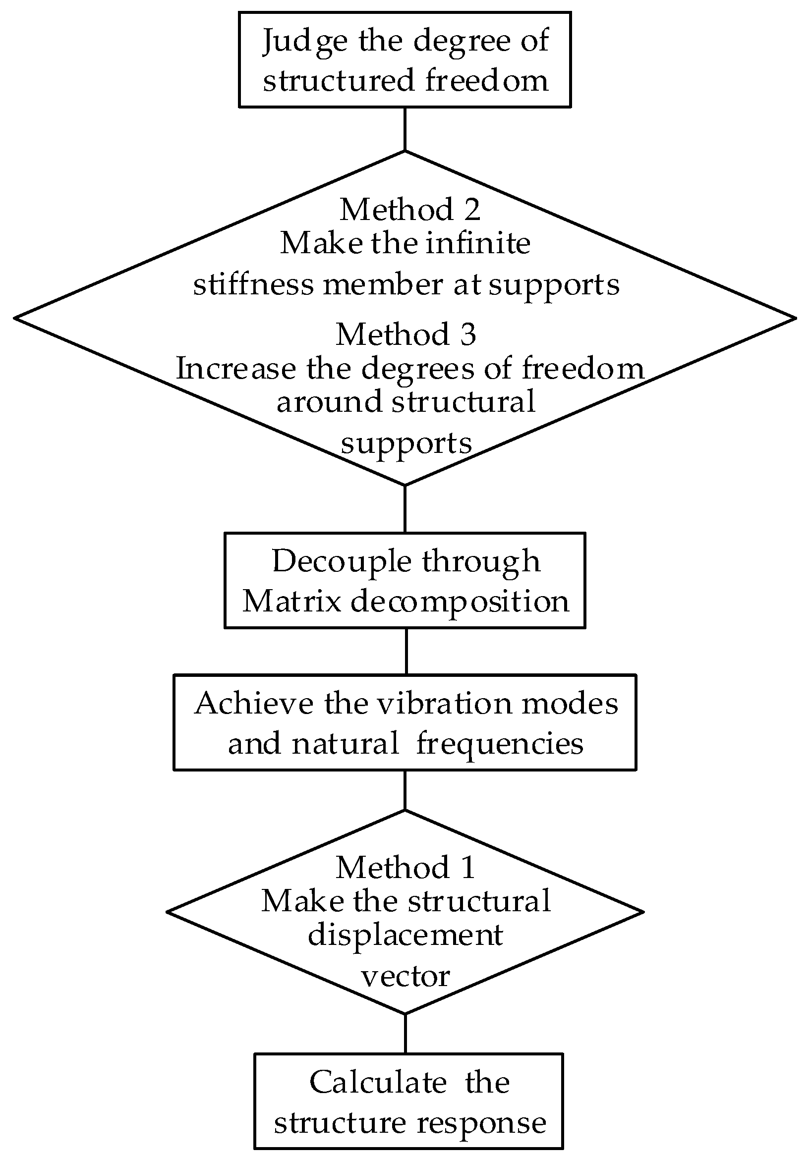
4.2. Method 1: Making the Structural Displacement Vector

This method is used to make the vector, ${\mathbf{X}}_a$, including all the translational displacements of the structure, that is,

$${\mathbf{X}}_a=\left\{\begin{array}{l}\mathbf{X}\\ {\mathbf{X}}_g\end{array}\right\},$$

(20)

where ${\mathbf{X}}_a$ is called the translational displacement vector. The transform vector, ${\mathbf{q}}_a$, is also divided into two parts corresponding to ${\mathbf{X}}_a$

$${\mathbf{q}}_a=\left\{\begin{array}{l}\mathbf{q}\\ {\mathbf{q}}_g\end{array}\right\},$$

(21)

where $\mathbf{q}$ and ${\mathbf{q}}_g$ correspond to $\mathbf{X}$ and ${\mathbf{X}}_g$. Hence, when ${\mathbf{q}}_a$ and ${\mathbf{X}}_a$ replace $\mathbf{q}$ and $\mathbf{X}$ in Equation (11), the new expression of the structural response, $z\left(t\right)$, can be written as

$$z\left(t\right)={\mathbf{q}}_a{}^T{\mathbf{X}}_a={\left\{\begin{array}{l}\mathbf{q}\\ {\mathbf{q}}_g\end{array}\right\}}^T\left\{\begin{array}{l}{\mathbf{X}}^s+{\mathbf{X}}^d\\ {\mathbf{X}}_g\end{array}\right\}={\mathbf{q}}^T\left({\mathbf{X}}^s+{\mathbf{X}}^d\right)+{\mathbf{q}}_g{}^T{\mathbf{X}}_g.$$

(22)

Then, Equation (23) can be yielded by substituting ${\mathbf{X}}^s=\mathbf{R}{\mathbf{X}}_g$ and ${\mathbf{X}}^d={\displaystyle \sum _{j=1}^n{\displaystyle \sum _{k=1}^m{\mathsf{\phi }}_j{\beta }_{jk}}}{\delta }_{jk}\left(t\right)$ into Equation (22)

$$z\left(t\right)={\displaystyle \sum _{k=1}^m\left(q_{gk}+a_k\right)x_{gk}+{\displaystyle \sum _{k=1}^m{\displaystyle \sum _{j=1}^n{b}_{jk}{\delta }_{jk}}}}.$$

(23)

If $\left(q_{gk}+a_k\right)$ in Equation (23) is written as

$$c_k=q_{gk}+a_k=q_{gk}+{\mathit{q}}^T{r}_k,$$

(24)

Equation (22) can be simplified as Equation (25)

$$z\left(t\right)={\displaystyle \sum _{k=1}^m{c}_k{x}_{gk}+{\displaystyle \sum _{k=1}^m{\displaystyle \sum _{j=1}^n{b}_{jk}{\delta }_{jk}}}},$$

(25)

and Equation (12) can be simplified as Equation (26)

$$\begin{array}{ll}{\mu }_{\left|z_{\max }\right|}=& [{\displaystyle \sum _{k=1}^m{\displaystyle \sum _{l=1}^m{c}_k{c}_l{\rho }_{x_{gk}{x}_{gl}}{\mu }_{x_{gk,\max }}{\mu }_{x_{gl,\max }}+2{\displaystyle \sum _{k=1}^m{\displaystyle \sum _{l=1}^m{\displaystyle \sum _{j=1}^n{c}_k{b}_{lj}{\rho }_{x_{gk}{\ddot{x}}_{glj}}{D}_l\left({\omega }_j,{\xi }_j\right)}}}}}\\ & {+{\displaystyle \sum _{k=1}^m{\displaystyle \sum _{l=1}^m{\displaystyle \sum _{i=1}^n{\displaystyle \sum _{j=1}^n{b}_{ki}{b}_{lj}{\rho }_{{\ddot{x}}_{gki}{\ddot{x}}_{glj}}}{\mu }_{x_{gk,\max }}{D}_k\left({\omega }_i,{\xi }_i\right)D_j\left({\omega }_j,{\xi }_j\right)}}}]}^{1/2}\end{array}$$

(26)

It should be noted that Equation (26) includes the effect caused by the displacements at the structural support degrees of freedom, so that this method could be considered as the best one.

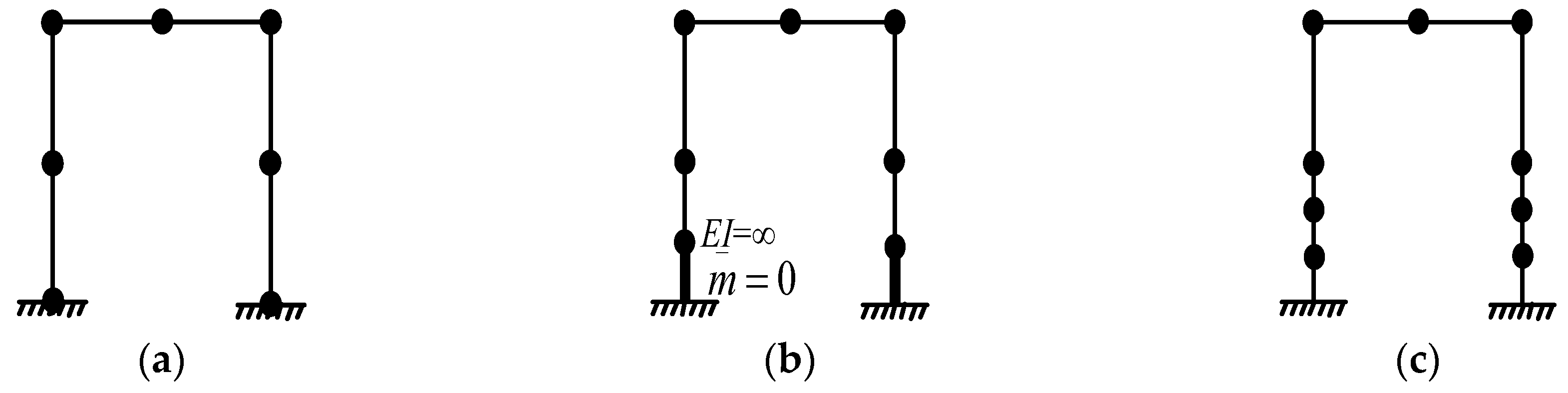
4.3. Method 2: Making the Infinite Stiffness Member at Supports

Considering the contribution of displacements at structural supports to the structural response, this method adopts making the infinite stiffness and massless member (unit bars) at supports (Figure 1b). The structural degrees of freedom at supports are changed into the non-support degrees of freedom. The structural vibration characteristics and the input of ground motion remain the same as those in the original model. This method considers the response caused by the structural support degrees of freedom without increasing the calculation. However, this method is not applicable for the structures with hinge supports, because the rotating displacements at both ends of the infinite stiffness member no longer remain completely consistent.

4.4. Method 3: Increasing the Degrees of Freedom around Structural Supports

This method is used to increase the degrees of freedom around structural supports (Figure 1c). All or almost all contributions of the displacements at the structural supports to the structural response could be substituted by the degrees of freedom near the supports. However, this method could result in an obvious increase of computation.

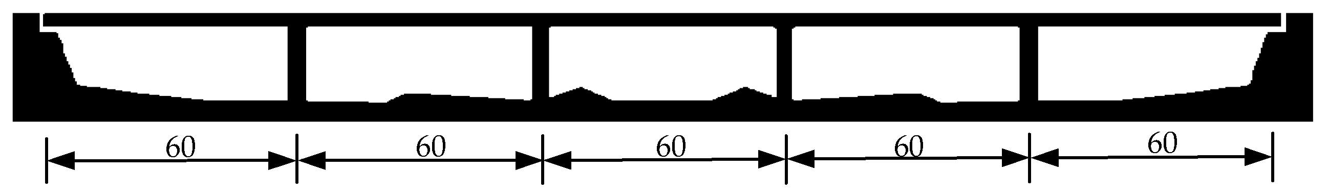
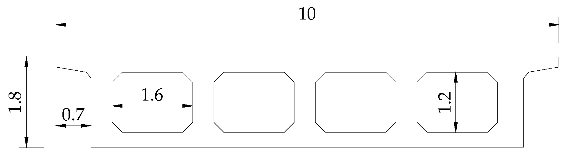
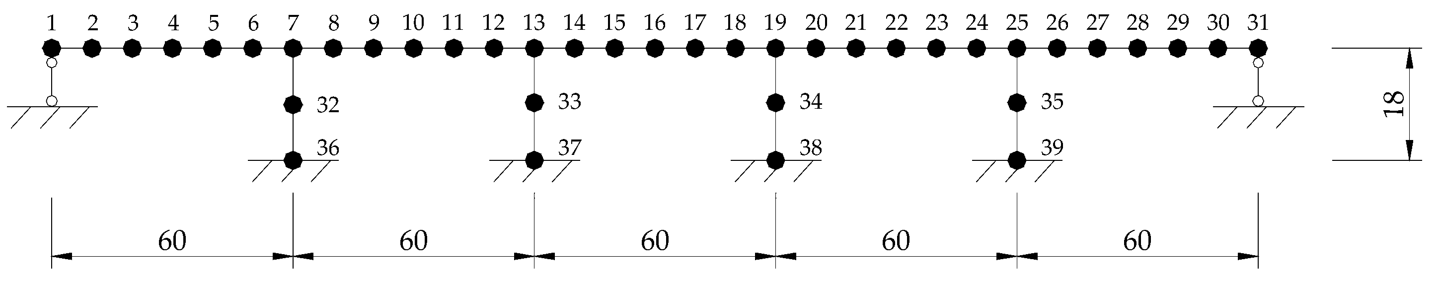
5. The Verification of the Modified MSRS Method

Here, a five-span reinforced concrete bridge is modeled as a 2-D frame system shown in Figure 2, which is used to verify the modified MSRS method in comparison with the original MSRS method. The distributions of the bridge mass and stiffness are homogeneous. Each span is 60 m and the width of the main bridge is 10 m. The girder consists of four single-box pre-stressed concrete continuous box girders, as shown in Figure 3. The four main piers are rectangular reinforced concrete piers with the same cross sections of 1.8 m × 2.4 m, the same heights of 18.0 m, and the same damping radios of ξ₁ = ξ₂ = 0.02.

The planar discrete model of the bridge used for calculating the structural responses is shown in Figure 4.

Figure 5 shows the first six dissymmetric or symmetric vibration modes of the bridges because of the symmetric structure.

The following section will firstly verify the shortcoming of the Complete Quadratic Combination (CQC) method in comparison with the MSRS method through numerically analyzing the response of the bridge under horizontal coherent or incoherent ground motion excitations as the stationary random process. Then, the modified MSRS method is calculated in the following process shown in Figure 6 and compared with the MSRS method using the same calculating example.

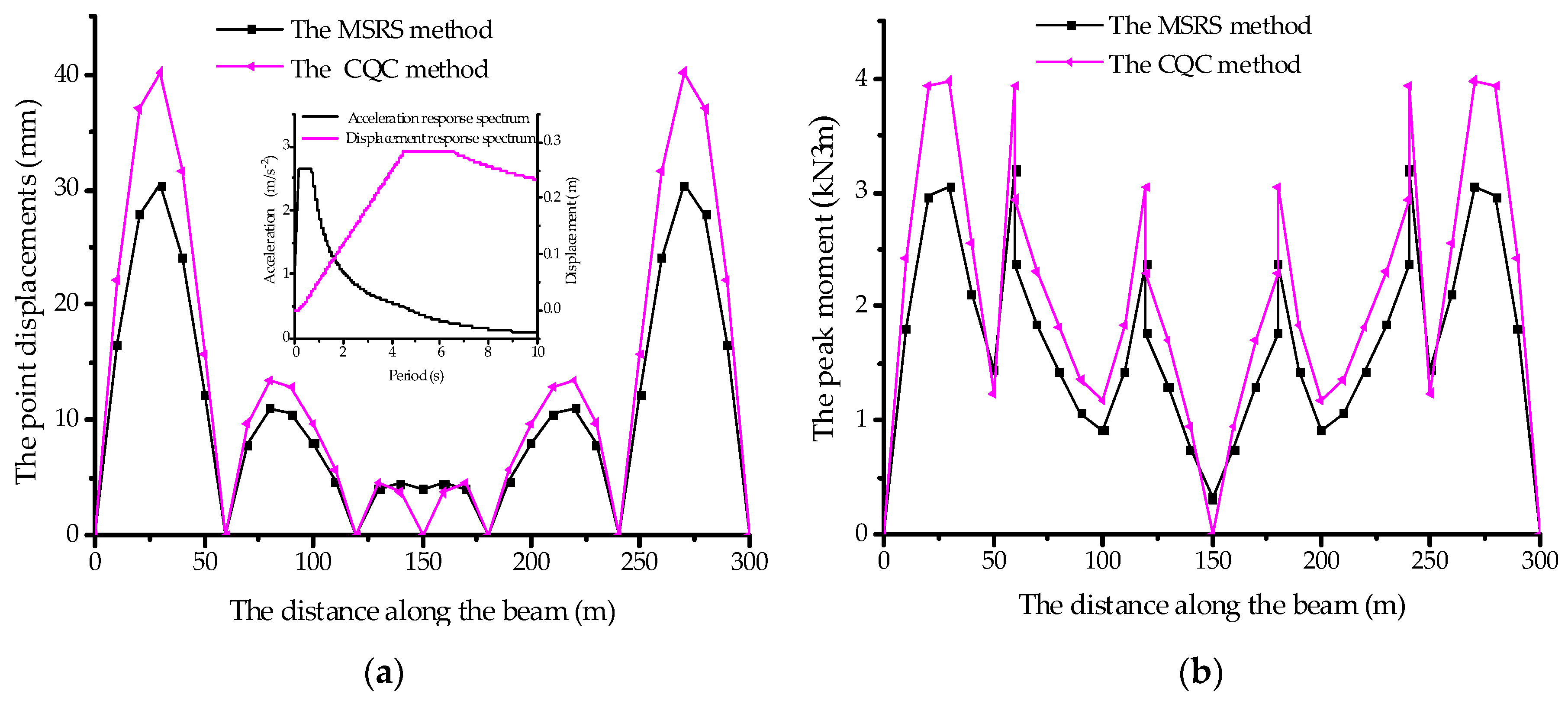
5.1. Comparison of the MSRS Method with the CQC Method

Figure 7a,b show the peak displacements and bending moments at the individual points along the length of the main beam calculated by the MSRS and CQC method in the case that the site is the Category IV and the ground movement intensity is the Level 9. The response spectrum of the case is shown in Figure 7a and the correlation coefficient, ${\rho }_{ij}$ between mode i and j for the CQC method is calculated by Equation (27)

$${\rho }_{ij}=\frac{8\sqrt{{\xi }_i{\xi }_j}\left({\xi }_i+r{\xi }_j\right)r^{3/2}}{{\left(1-r^2\right)}^2+4{\xi }_i{\xi }_{j}r\left(1+r^2\right)+4\left({\xi }_i^2+{\xi }_j^2\right)r^2},$$

(27)

where r is calculated by Equation (28)

$$r=\frac{{\omega }_i}{{\omega }_j}$$

(28)

where ω_i is the frequency for mode i.

It is shown that the structural response calculated using the MSRS method is less than that obtained from the CQC method (Figure 7), because the MSRS method considers the wave passage effect and the CQC method does not involve this effect instead. This implies that the result calculated using the CQC method becomes conservative. Besides, the passage effect, which leads to the different phases of the seismic wave at individual supports, at the same time, might reduce the structural response in some cases. It can be seen that the results calculated by the two methods are obviously different at the middle point of the main beam. The bending moment and the biggest displacement at this point calculated by the CQC method are zero under coherent ground motion, while the corresponding values calculated by the MSRS method are 322 kN∙m and 4.075 mm, respectively. This is because the MSRS method includes the pseudo static effect derived from the displacement differences of individual supports and the CQC method does not introduce this pseudo static displacement instead. This further indicates that the MSRS method can more accurately reflect the structural response than the CQC method does.

5.2. Comparison of the Modified MSRS Method with the MSRS Method

Table 1. The comparison of bending moments from the MSRS method and the modified MSRS method.

Position	Bending Moment M (×103 kN∙m)
Method	The MSRS Method	The Modified MSRS Method 1 1	The Modified MSRS Method 2 1
Girder point 4	2.99	3.06	3.06
Girder point 10	1.06	1.06	1.06
Girder point 16	0.30	0.30	0.32
Pier point 7	14.30	39.50	39.50
Pier point 13	14.20	37.50	37.50
Pier point 32	35.40	1.36	1.36
Pier point 33	35.30	0.79	0.79

¹ The modified MSRS method 1 or 2 indicates Method 1 or 2.

lists the bending moments at the typical girder and pier points calculated by the existing MSRS method and the modified MRSR method utilizing Method 1 and 2. From Table 1, it can be seen that:

• The bending moment values and the peak bending moment at the girder points calculated by the two methods are almost the same;
• The bending moments at the points far from supports calculated by the two methods are close to each other;
• The bending moments at the points of the piers close to the supports calculated by the existing MSRS method are much different from those calculated by the modified MSRS method, with even the biggest deviation is up to several tens of times different. Clearly, the MSRS method is inaccurate in calculating the responses near the supports when compared with the modified MSRS method. Therefore, the comparison based on Table 1 validates the modified MSRS method.

6. The Spectrum Methods for Incoherent Ground Displacement Excitations

6.1. The Differential Equation of Motion for Incoherent Ground Displacement Excitations

Nowadays, the concentrated mass method has been widely applied in the dynamic analysis of structures, with the zero values for the off-diagonal elements in the mass matrix. Thus, a differential equation of motion can be written as

$$\left[\begin{array}{cc}\mathbf{M}& \mathbf{0}\\ \mathbf{0}& {\mathbf{M}}_g\end{array}\right]\left\{\begin{array}{l}\ddot{\mathbf{X}}\\ {\ddot{\mathbf{X}}}_g\end{array}\right\}+\left[\begin{array}{cc}\mathbf{C}& \mathbf{0}\\ \mathbf{0}& {\mathbf{C}}_g\end{array}\right]\left\{\begin{array}{l}\dot{\mathbf{X}}\\ {\dot{\mathbf{X}}}_g\end{array}\right\}+\left[\begin{array}{cc}\mathbf{K}& {\mathbf{K}}_c\\ {\mathbf{K}}_c^T& {\mathbf{K}}_g\end{array}\right]\left\{\begin{array}{l}\mathbf{X}\\ {\mathbf{X}}_g\end{array}\right\}=\left\{\begin{array}{l}\mathbf{0}\\ \mathbf{F}\end{array}\right\},$$

(29)

in which all the items are the same meanings as those in Equation (10). Usually, an orthogonal damping coefficient matrix is manually constructed, when using the mode-superposition method to solve the differential equation of motion. Here, the off-diagonal elements in the damping matrix are also treated as zero. If the calculated values do not agree with the experimental values, the calculating model could be improved by changing the mode damping ratio.

For the concentrated mass system, the mass matrix is reasonable, like that in Equation (29). For the coherent mass system, the mass matrix in Equation (29) is also applicable when the original model 1 in Figure 1a is modified into that for the modified MSRS method by utilizing Method 1 in Figure 1b. Also, for the model in Figure 1b, the support degrees of freedom always maintain the same displacements with the non-support degrees of freedom, which are connected with the supports. Hence, it is reasonable to assume that the coupling damping coefficient is zero for the support and non-support degrees of freedom.

6.2. The Power Spectrum Method (Solution)

The first differential equation of motion in Equation (29) is written as Equation (30)

$$\mathbf{M}\ddot{\mathbf{X}}+\mathbf{C}\dot{\mathbf{X}}+\mathbf{K}\mathbf{X}+{\mathbf{K}}_c{\mathbf{X}}_g=\mathbf{0}.$$

(30)

Also, the solution of Equation (30) can be supposed as the form expressed by Equation (31)

$$\mathbf{X}=\mathsf{\Phi }\mathbf{u}={\displaystyle \sum _{j=1}^n{\mathsf{\phi }}_j}\cdot u_j,$$

(31)

where $\mathsf{\Phi }=\left[{\mathsf{\phi }}_1,{\mathsf{\phi }}_2,\cdots {\mathsf{\phi }}_n\right]$ is the mode matrix; ${\mathsf{\phi }}_j$ is the column vector of the jth mode; $u_j$ is the generalized coordinate of the jth mode. Substituting Equation (31) into Equation (30) and then multiplying ${\mathsf{\phi }}_j^T$, Equations (32) and (33) can be obtained by using the mode composition method

$${\ddot{u}}_j+\frac{{\mathsf{\phi }}_j^T\mathbf{C}{\mathsf{\phi }}_j}{{\mathsf{\phi }}_j^T\mathbf{M}{\mathsf{\phi }}_j}\cdot {\dot{u}}_j+\frac{{\mathsf{\phi }}_j^T\mathbf{K}{\mathsf{\phi }}_j}{{\mathsf{\phi }}_j^T\mathbf{M}{\mathsf{\phi }}_j}\cdot u_j=\frac{-{\mathsf{\phi }}_j^T{\mathbf{K}}_c}{{\mathsf{\phi }}_j^T\mathbf{M}{\mathsf{\phi }}_j}\cdot {\mathbf{X}}_g,$$

(32)

$${\ddot{u}}_j+2{\zeta }_j{\omega }_j{\dot{u}}_j+{\omega }_j^2{u}_j={\displaystyle \sum _{k=1}^m{\beta }_{jk}}{x}_{gk},$$

(33)

where $x_{gk}\left(t\right)$ is the ground motion displacement at support k at the time t; ${\beta }_{jk}$ denotes the participation factor of the jth mode at support k, as expressed by Equation (34)

$$\left\{{\beta }_{j1},{\beta }_{j2}\cdots {\beta }_{jm}\right\}=\frac{-{\mathsf{\phi }}_j^T{\mathbf{K}}_c}{{\mathsf{\phi }}_j^T\mathbf{M}{\mathsf{\phi }}_j},$$

(34)

where m is the number of supports. Hence, Equation (33) can be converted to Equation (35) using

$$u_j={\displaystyle \sum _{k=1}^m{\beta }_{jk}{\delta }_{jk}},{\ddot{\delta }}_j+2{\zeta }_j{\omega }_j{\dot{\delta }}_j+{\omega }_j^2{\delta }_j=x_{gk},$$

(35)

$$\mathbf{X}={\displaystyle \sum _{j=1}^n{u}_j{\mathsf{\phi }}_j}={\displaystyle \sum _{j=1}^n{\displaystyle \sum _{k=1}^m{\beta }_{jk}}}{\delta }_{jk}{\mathsf{\phi }}_j,$$

(36)

where ${\delta }_{jk}$ is the generalized displacement at the kth support in the jth mode.

Now, z is supposed as a structural response and expressed by Equations (37)–(39) through the nodal displacement vector, $\mathbf{X}$

$$z={\mathbf{q}}^T\mathbf{X},$$

(37)

$$z={\displaystyle \sum _{j=1}^n{\displaystyle \sum _{k=1}^m{\beta }_{jk}{\mathbf{q}}^T{\mathsf{\phi }}_j}}{\delta }_{jk}={\displaystyle \sum _{j=1}^n{\displaystyle \sum _{k=1}^m{b}_{jk}}}{\delta }_{jk},$$

(38)

$$b_{jk}={\beta }_{jk}{\mathbf{q}}^T{\mathsf{\phi }}_j,$$

(39)

where ${\mathbf{q}}^T$ is the vector transferring displacement response to the other response; $b_{jk}$ is the combination factor. Response $z$ is a random process, and its self-power spectral density function can be obtained from the theory of random vibration, that is,

$$S_{zz}\left(\omega \right)={\displaystyle \sum _{k=1}^m{\displaystyle \sum _{l=1}^m{\displaystyle \sum _{i=1}^n{\displaystyle \sum _{j=1}^n{b}_{ki}{b}_{lj}{H}_i\left(i\omega \right)}}}}H\left(-i\omega \right)S_{x_{gk}{x}_{gl}}\left(i\omega \right),$$

(40)

where ${\omega }_i$ is the natural frequency to the ith mode; $i={\left(-1\right)}^{-\frac{1}{2}}$ is the unit imaginary number; $H_i\left(i\omega \right)={\left[{\omega }_i{}^2-{\omega }^2+2i{\zeta }_i{\omega }_i\omega \right]}^{-1}$ is the complex frequency response function of the ith mode; $H_j\left(-i\omega \right)={\left[{\omega }_j{}^2-{\omega }^2-2i{\zeta }_j{\omega }_j\omega \right]}^{-1}$ is the conjugation of the complex frequency response function of the jth mode; ${\zeta }_i$ is the structural damping ratio of the ith mode; $S_{x_{gk}{x}_{gl}}\left(i\omega \right)$ is the cross-power spectrum density function of the earthquake displacements on the ground at points k and l, which is obtained from the acceleration cross-power spectrum density function, $S_{{\ddot{x}}_{gk}{\ddot{x}}_{gl}}\left(i\omega \right)$. Furthermore, the variance of response $z$ can be calculated as

$${\sigma }_z^2={\displaystyle {\int }_{-\infty }^{+\infty }{S}_{zz}\left(\omega \right)}d\omega ={\displaystyle \sum _{k=1}^m{\displaystyle \sum _{l=1}^m{\displaystyle \sum _{i=1}^n{\displaystyle \sum _{j=1}^n{b}_{ki}{b}_{lj}{\displaystyle {\int }_{-\infty }^{+\infty }{H}_i\left(i\omega \right)}}}}}{H}_j\left(-i\omega \right)S_{x_{gk}{x}_{gl}}\left(i\omega \right)d\omega .$$

(41)

Now, ${\rho }_{{\delta }_{ki}{\delta }_{lj}}$ is used to express the correlation coefficient of the jth mode response, ${\delta }_{lj}$ under ground displacement, $x_{gl}\left(t\right)$ at support l and ${\sigma }_{{\delta }_{ki}}^2$ is used to express the variance of the ith mode response, ${\delta }_{ki}$ under ground displacement, $x_{gk}\left(t\right)$ at support k, then,

$${\rho }_{{\delta }_{ki}{\delta }_{lj}}=\frac{1}{{\sigma }_{{\delta }_{ki}{\delta }_{lj}}}{\displaystyle {\int }_{-\infty }^{\infty }{H}_i\left(i\omega \right)}{H}_j\left(-i\omega \right)S_{x_{gk}{x}_{gl}}\left(i\omega \right)d\omega ,$$

(42)

$${\sigma }_{{\delta }_{ki}}{}^2={{\displaystyle {\int }_{-\infty }^{\infty }\left|H_i\left(i\omega \right)\right|}}^2{S}_{x_{gk}{x}_{gk}}\left(\omega \right)d\omega .$$

(43)

Thus,

$${\sigma }_z^2={\displaystyle \sum _{k=1}^m{\displaystyle \sum _{l=1}^m{\displaystyle \sum _{i=1}^n{\displaystyle \sum _{j=1}^n{b}_{ki}{b}_{lj}{\rho }_{{\delta }_{ki}{\delta }_{lj}}{\sigma }_{{\delta }_{ki}}}}}}{\sigma }_{{\delta }_{lj}}.$$

(44)

According to ${\sigma }_{\dot{z}}^2={\displaystyle {\int }_{-\infty }^{+\infty }{\omega }^2{S}_{zz}\left(i\omega \right)d\omega }$, the variance of the first derivative of $z\left(t\right)$ is given as

$${\sigma }_{\dot{z}}^2={\displaystyle \sum _{k=1}^m{\displaystyle \sum _{l=1}^m{\displaystyle \sum _{i=1}^n{\displaystyle \sum _{j=1}^n{b}_{ki}{b}_{lj}{\displaystyle {\int }_{-\infty }^{+\infty }{\omega }^2{H}_i\left(i\omega \right)}}}}}{H}_j\left(-i\omega \right)S_{x_{gk}{x}_{gl}}\left(i\omega \right)d\omega .$$

(45)

Furthermore, the average frequency, $\overline{\omega }$ and the average rate, $\gamma$ of $z\left(t\right)$ beyond zero are calculated by Equations (46) and (47)

$$\overline{\omega }=\frac{{\sigma }_{\dot{z}}^{}}{{\sigma }_z^{}},$$

(46)

$$\gamma =\frac{\overline{\omega }}{\pi }.$$

(47)

Meanwhile, the peak response factors, $p_z$ and $q_z$ of $z\left(t\right)$ can be calculated by Equations (48) and (49)

$$p_z=\sqrt{2\ln \left(\gamma T_d\right)}+\frac{0.5772}{\sqrt{2\ln \left(\gamma T_d\right)}},$$

(48)

$$q_z=\frac{\pi }{\sqrt{6}}\frac{1}{\sqrt{2\ln \left(\gamma T_d\right)}},$$

(49)

where $T_d$ is the duration of an earthquake.

Finally, the mean value and mean value square deviation of the absolute peak value, $\left|z_{\max }\right|$ for the structural response, $z\left(t\right)$ during the period, $\left[0,T_d\right]$ can be obtained as

$${\mu }_{\left|z_{\max }\right|}=p_z{\sigma }_z,$$

(50)

$${\sigma }_{\left|z_{\max }\right|}=q_z{\sigma }_z.$$

(51)

Once ${\mu }_{\left|z_{\max }\right|}$ and ${\sigma }_{\left|z_{\max }\right|}$ are determined, the mean and variance of the peak response of the structure can be obtained.

6.3. The Response Spectrum Method for Incoherent Ground Displacement Excitations

By substituting Equation (45) into Equation (46), ${\mu }_{z_{\max }}$ can be written as

$${\mu }_{z_{\max }}={\left({\displaystyle \sum _{k=1}^m{\displaystyle \sum _{l=1}^m{\displaystyle \sum _{i=1}^n{\displaystyle \sum _{j=1}^n{b}_{ki}{b}_{lj}{\rho }_{{\delta }_{ki}{\delta }_{lj}}{p}_z^2{\sigma }_{{\delta }_{ki}}}}}}{\sigma }_{{\delta }_{lj}}\right)}^{\frac{1}{2}}.$$

(52)

According to the definition of the response spectrum, a response spectrum value equals to average response of a single degree-of-freedom system subjected to the same ground excitation. Hence,

$$D_k\left({\omega }_i,{\zeta }_i\right)=p_{{\delta }_{ki}}{\sigma }_{{\delta }_{ki}}.$$

(53)

Substituting Equation (53) into Equation (52), ${\mu }_{z_{\max }}$ can be written as

$${\mu }_{z_{\max }}={\left({\displaystyle \sum _{k=1}^m{\displaystyle \sum _{l=1}^m{\displaystyle \sum _{i=1}^n{\displaystyle \sum _{j=1}^n{b}_{ki}{b}_{lj}{\rho }_{{\delta }_{ki}{\delta }_{lj}}\frac{p_z^2}{p_{{\delta }_{ki}}{p}_{{\delta }_{lj}}}{D}_k\left({\omega }_i,{\zeta }_i\right)}}}}{D}_l\left({\omega }_j,{\zeta }_j\right)\right)}^{\frac{1}{2}}.$$

(54)

Because $p_z^2/\left(p_{{\delta }_{ki}}{p}_{{\delta }_{lj}}\right)$ is near to 1, then

$${\mu }_{z_{\max }}={\left({\displaystyle \sum _{k=1}^m{\displaystyle \sum _{l=1}^m{\displaystyle \sum _{i=1}^n{\displaystyle \sum _{j=1}^n{b}_{ki}{b}_{lj}{\rho }_{{\delta }_{ki}{\delta }_{lj}}{D}_k\left({\omega }_i,{\zeta }_i\right)}}}}{D}_l\left({\omega }_j,{\zeta }_j\right)\right)}^{\frac{1}{2}}.$$

(55)

Equation (55) is the expression of the mean of the structural peak response under incoherent ground displacement excitation.

In consideration of the effect of the support degrees of freedom, the expression of the mean response spectrum method should be modified. Therefore, a structural response, $z\left(t\right)$ can be expressed by the nodal displacement, ${\mathbf{X}}_a$ and ${\mathit{q}}_a$,

$$z\left(t\right)={\mathbf{q}}_a{}^T{\mathbf{X}}_a={\left\{\begin{array}{l}\mathbf{q}\\ {\mathbf{q}}_g\end{array}\right\}}^T\left\{\begin{array}{l}\mathbf{X}\\ {\mathbf{X}}_g\end{array}\right\}={\mathbf{q}}^T\mathbf{X}+{\mathbf{q}}_g{}^T{\mathbf{X}}_g,$$

(56)

$$z\left(t\right)={\displaystyle \sum _{k=1}^m{q}_{gk}}{x}_{gk}\left(t\right)+{\displaystyle \sum _{j=1}^n{\displaystyle \sum _{k=1}^m{\beta }_{jk}{\mathbf{q}}^T{\mathsf{\phi }}_j{\delta }_{jk}\left(t\right)}}={\displaystyle \sum _{k=1}^m{q}_{gk}{x}_{gk}\left(t\right)}+{\displaystyle \sum _{j=1}^n{\displaystyle \sum _{k=1}^m{b}_{jk}{\delta }_{jk}}}\left(t\right),$$

(57)

$$\begin{array}{ll}{\mu }_{\left|z,\max \right|}=& [{\displaystyle \sum _{k=1}^m{\displaystyle \sum _{l=1}^m{q}_{gk}{q}_{gl}{\rho }_{x_{gk}{x}_{gl}}{\mu }_{x_{gk,\max }}{\mu }_{x_{gl,\max }}+2{\displaystyle \sum _{k=1}^m{\displaystyle \sum _{l=1}^m{\displaystyle \sum _{j=1}^n{q}_{gk}{b}_{lj}{\rho }_{x_{gk}{\ddot{x}}_{lj}}{D}_l\left({\omega }_j,{\zeta }_j\right)}}}}}\\ & {+{\displaystyle \sum _{k=1}^m{\displaystyle \sum _{l=1}^m{\displaystyle \sum _{i=1}^n{\displaystyle \sum _{j=1}^n{b}_{ki}{b}_{lj}{\rho }_{{\ddot{x}}_{gki}{\ddot{x}}_{glj}}}{\mu }_{x_{gk,\max }}{D}_k\left({\omega }_i,{\zeta }_i\right)D_l\left({\omega }_j,{\zeta }_j\right)}}}]}^{\frac{1}{2}}\end{array}$$

(58)

where q_gk is the conversion factor of x_gk in the conversion vector, ${\mathbf{q}}^T$.

It should be noted that the structural response derived from Equations (57) and (58) needs to be used to construct the structural displacement vector, ${\mathbf{X}}_a$ like the modified MSRS method utilizing Method 1.

6.4. The Simplified Power Spectrum Method

Here, a simplification of the peak factor, p_z or q_z, is made through the analysis of the structural response in the example above. The site condition of the structure is the Category Ⅳ and the seismic intensity Ⅸ. Structural damping ratio is supposed as 0.02. Structural response mean values and variance peak factors are calculated by Equations (44), (45), (48), and (49), as listed in

Table 2. The structural peak response values.

Position	Peak Factor		Position	Peak Factor
	${\mathit{p}}_{\mathit{z}}$	${\mathit{q}}_{\mathit{z}}$		${\mathit{p}}_{\mathit{z}}$	${\mathit{q}}_{\mathit{z}}$
VD 1 at Point 2	2.79	0.50	BBM at the left of Point 13	2.72	0.52
VD at Point 3	2.78	0.50	BBM at the right of Point 13	2.72	0.52
VD at Point 4	2.78	0.50	BBM at Point 14	2.72	0.52
VD at Point 5	2.77	0.50	BBM at Point 15	2.73	0.51
VD at Point 6	2.76	0.51	BBM at Point 16	2.80	0.50
VD at point 8	2.75	0.51	PBM 2 at Point 7	2.76	0.51
VD at Point 9	2.78	0.50	PBM at Point 13	2.70	0.52
VD at Point 10	2.81	0.49	PBM at Point 32	2.73	0.51
VD at Point 11	2.82	0.49	PBM at Point 33	2.72	0.52
VD at Point 12	2.78	0.50	SBM 2 at Point 36	2.71	0.52
VD at Point 14	2.72	0.51	SBM at Point 37	2.70	0.52
VD at Point 15	2.73	0.51	SF 3 in Beam 1–2	2.80	0.50
VD at Point 16	2.79	0.50	SF in Beam 2–3	2.79	0.50
HD 1 at bridge deck	2.70	0.52	SF in Beam 3–4	2.69	0.52
HD at Point 32	2.70	0.52	SF in Beam 4–5	2.80	0.50
HD at Point 33	2.69	0.52	SF in Beam 5–6	2.80	0.50
HD at Point 36	2.73	0.51	SF in Beam 6–7	2.80	0.50
HD at Point 37	2.69	0.52	SF in beam 7–8	2.82	0.49
BBM 2 at Point 2	2.79	0.50	SF in Beam 8–9	2.79	0.50
BBM at Point 3	2.79	0.50	SF in beam 9–10	2.72	0.51
BBM at Point 4	2.79	0.50	SF in Beam 10–11	2.72	0.52
BBM at Point 5	2.77	0.50	SF in beam 11–12	2.75	0.51
BBM at Point 6	2.71	0.52	SF in Beam 12–13	2.78	0.50
BBM at the left of Point 7	2.79	0.50	SF in Beam 13–14	2.73	0.51
BBM at the right of Point 7	2.73	0.51	SF in Beam 14–15	2.72	0.51
BBM at Point 8	2.71	0.52	SF in Beam 15–16	2.72	0.51
BBM at Point 9	2.75	0.51	SF in Pier 7–32	2.73	0.51
BBM at Point 10	2.82	0.49	SF in Beam 13–33	2.70	0.52
BBM at Point 11	2.78	0.50	SF in Beam 32–36	2.73	0.51
BBM at Point 12	2.70	0.52	SF in Beam 33–37	2.70	0.52

¹ VD and HD represent the vertical displacement and horizontal displacement, respectively; ² BBM, PBM, and SBM represent the beam bending moment, pier bending moment, and support bending moment, respectively; ³ SF represents the shearing force.

. In Table 2, the mean values are ${\mu }_{p_z}=$ 2.752 and ${\mu }_{q_z}=$ 0.508; the standard deviations are ${\sigma }_{p_z}=$ 0.0400 and ${\sigma }_{q_z}=$ 0.00884; the variation coefficients are ${\delta }_{p_z}=$ 0.015 and ${\delta }_{q_z}=$ 0.017; the largest difference between $p_z$ and ${\mu }_{p_z}$ is 2.75%; the largest difference between $q_z$ and ${\mu }_{q_z}$ is 3.22%. The calculating result indicates that the mean values and variance peak factors change to a small extent. Therefore, for a simplification, the peak factors to structural responses can be approximately calculated according to the seismic and structural features.

The mean value, $p_g$ and the peak variance factor, $q_g$ of ground motion displacement can be calculated by substituting Equations (59) and (60) into Equations (48), (49), (50), and (51)

$${\lambda }_m={\displaystyle {\int }_{-\infty }^{\infty }{\omega }^{m}S\left(\omega \right)}d\omega ,$$

(59)

$$\overline{\omega }=\frac{\sqrt{{\lambda }_2}}{\sqrt{{\lambda }_0}}.$$

(60)

The calculated result for Point 9 is $p_g$ = 2.533 and $q_g$ = 0.563, respectively, near to the corresponding values of the structural peak response factors, $p$ and $q$, as listed in Table 2. But, the difference still exists between the ground displacement factors and structural peak response factors. This difference seems to be because $p_g$ and $q_g$ do not include structural damping and natural frequency characteristics, which are considered in $p_z$ and $q_z$. However, since $p_z$ and $q_z$ do not obviously change with the damping ratios, as listed in

Table 3. The peak response factor of beam bending moment at Point 9.

$\mathit{\zeta }$	${\mathit{p}}_{\mathit{z}}$	${\mathit{q}}_{\mathit{z}}$
0.05	2.72	0.51
0.05	2.72	0.52
0.04	2.73	0.51
0.04	2.73	0.51
0.03	2.74	0.51
0.03	2.74	0.51
0.02	2.75	0.51
0.01	2.76	0.51

, the difference is not caused by the damping ratio, $\zeta$. Hence, it is not a reasonable choice to replace the peak response factor using those deduced in the case of ground displacement exercitation.

The analytical results above imply a different approach for describing structural peak response factors. This approach could be easily obtained through the generalized single-degree-of-freedom (GSDOF) system with lumped mass under seismic displacement action. The peak response factors of GSDOF systems corresponding to natural frequencies of the structure, $p_d$ and $q_d$, reflect the collective effect of the ground displacement, structural frequency, and damping characteristics. Therefore, $p_d$ and $q_d$ should be closer to the structural peak response factors. Equation (61) (reference) is adopted for the mth order spectral moment of the GSDOF system corresponding to the jth mode

$${\lambda }_{m,j}={\displaystyle {\int }_{-\infty }^{\infty }{\omega }^m{H}_j\left(i\omega \right)H_j\left(-i\omega \right)S\left(\omega \right)}d\omega ,$$

(61)

where S(ω) is the power spectrum density function of ground displacement. For the structural model in Figure 4, the mean value and peak variance factors of GSDOF systems, $p_d$ and $q_d$ can be calculated by Equations (60), (61), (48), (49), (50), and (51), and the result is shown in

Table 4. The peak factors of generalized single-degree-of-freedom (GSDOF) systems.

$\mathit{\omega }$	${\mathit{p}}_{\mathit{d}}$	${\mathit{q}}_{\mathit{d}}$	$\mathit{\omega }$	${\mathit{p}}_{\mathit{d}}$	${\mathit{q}}_{\mathit{d}}$
ω1 = 4.81	2.71	0.51	ω6 = 8.97	2.81	0.49
ω2 = 5.61	2.75	0.50	ω7 = 18.71	2.65	0.53
ω3 = 6.11	2.77	0.50	ω8 = 18.88	2.65	0.53
ω4 = 6.92	2.79	0.49	ω9 = 20.93	2.62	0.53
ω5 = 7.98	2.81	0.49	ω10 = 23.03	2.60	0.54

.

Now, ${\mu }_{p_d}=$ 2.750 and ${\mu }_{q_d}=$ 0.509 can be obtained by calculating the average value of the peak response factors for the first three vibration modes. Clearly, they are very close to the mean values of the structural peak response factors, ${\mu }_{p_z}=$ 2.752 and ${\mu }_{q_z}=$ 0.508. The greatest difference between ${\mu }_{p_d}$ and $p_z$, or ${\mu }_{q_d}$ and $q_z$, is 2.8% or 3.3%; if conducting similar calculation is conducted for the first six modes, ${\mu }_{p_d}=$ 2.779 and ${\mu }_{q_d}=$ 0.502. The greatest difference between ${\mu }_{p_d}$ and $p_z$, or ${\mu }_{q_d}$ and $q_z$, is 3.1% or 3.8%. Hence, structural peak response factors can be replaced using the mean peak response factor for the first k GSDOF systems, that is,

$${\overline{p}}_z=\frac{1}{k}{\displaystyle \sum _{j=1}^k{p}_{d,j}},$$

(62)

$${\overline{p}}_z=\frac{1}{k}{\displaystyle \sum _{j=1}^k{p}_{d,j}},$$

(63)

where p_d,j and q_d,j are calculated by Equations (59), (60), (48), (49), (50), and (51); k is the order number, which has the biggest contribution to the structural response and is taken as 3~6 for the example in Figure 4. ${\overline{p}}_z$ and ${\overline{q}}_z$ are the collective peak response factors based on the incoherent ground displacement input. Correspondingly, the response spectrum method using ${\overline{p}}_z$ and ${\overline{q}}_z$ is called as the collective response spectrum method. Now, the results above can be summarized as a few points:

• ${\overline{p}}_z$ and ${\overline{q}}_z$ in Equations (62) and (63) simplify the peak response factors, $p_z$ and $q_z$, in Equations (48) and (49). ${\overline{p}}_z$ and ${\overline{q}}_z$ can calculate the peak response and the variance of the peak response in the structural linear-elastic stage under incoherent ground motion.
• ${\overline{p}}_z$ and ${\overline{q}}_z$ have three merits when compared with the peak response factors, $p_z$ and $q_z$: less computation, less process extent in simplifying and approximating, and without involving in the response spectrum.
• When compared with the existing power spectrum method introduced above, the collective response spectrum method reduces the computational effort by about 50%.

6.5. The Validity of the Power Spectrum/Collective Response Spectrum Methods

In order to further verify the power spectrum method (Equations (49) and (51)), the simplified power spectrum method (Equations (62) and (63)) and the collective response spectrum method (Equations (48), (49), and (58)), the modified MSRS method (Equations (12) and (13)) is exampled to calculate the structural response. The calculated results are listed in

Table 5. The comparison of bending moments calculated by the four methods.

Structural Response	The MSRS Method		The Power Spectrum Method		The Simplified Power Spectrum Method	The Collective Response Spectrum Method
	${\mathit{\sigma }}_{\left|\mathit{M},\mathbf{max}\right|}{}^2$	${\mathit{\mu }}_{\left|\mathit{M},\mathbf{max}\right|}$	${\mathit{\sigma }}_{\left|\mathit{M},\mathbf{max}\right|}$	${\mathit{\mu }}_{\left|\mathit{M},\mathbf{max}\right|}$	${\mathit{\mu }}_{\left|\mathit{M},\mathbf{max}\right|}$	${\mathit{\mu }}_{\left|\mathit{M},\mathbf{max}\right|}$
BBM 1 at Point 02	0.61	1.81	0.62	1.54	1.71	1.76
BBM at Point 03	1.00	2.97	1.01	2.51	2.78	2.91
BBM at Point 04	1.02	3.06	1.03	2.54	2.82	3.02
BBM at Point 05	0.67	2.12	0.67	1.66	1.85	2.10
BBM at Point 06	0.31	1.45	0.43	1.04	1.19	1.14
BBM at the left of Point 07	0.97	3.20	1.10	2.72	3.01	2.72
BBM at the right of Point 07	0.76	2.37	0.88	2.14	2.42	2.76
BBM at Point 08	0.61	1.84	0.69	1.66	1.90	2.21
BBM at Point 09	0.47	1.43	0.51	1.24	1.40	1.58
BBM at Point 10	0.34	1.06	0.34	0.86	0.94	0.90
BBM at Point 11	0.29	0.92	0.34	0.83	0.92	0.92
BBM at Point 12	0.48	1.44	0.59	1.41	1.62	1.83
BBM at the left of Point 13	0.80	2.38	0.93	2.25	2.57	2.90
BBM at the right of Point 13	0.58	1.77	0.75	1.80	2.05	2.19
BBM at point 14	0.43	1.31	0.55	1.32	1.50	1.60
BBM at Point 15	0.24	0.75	0.30	0.73	0.83	0.87
BBM at Point 16	0.06	0.32	0.07	0.17	0.19	0.14
PBM at Point 07	1.20	3.95	1.53	3.75	4.21	3.91
PBM at Point 13	1.28	3.75	1.59	3.80	4.37	4.90
PBM at Point 32	0.44	1.36	0.47	1.15	1.31	1.52
PBM at Point 33	0.24	0.79	0.31	0.74	0.85	0.90
PBM at Point 36	1.59	5.32	2.09	5.04	5.75	6.00
PBM at Point 37	1.77	5.30	2.23	5.35	6.14	6.82

¹ BBM represents beam bending moment and PBM pier bending moment; ² M denotes bending moment.

and

Table 6. The comparison of displacements calculated by the four methods.

Structural Response (mm)	The MSRS Method		The Power Spectrum Method		The Simplified Power Spectrum Method	The Collective Response Spectrum Method
	${\mathit{\sigma }}_{\left|\mathit{z},\mathbf{max}\right|}$	${\mathit{\mu }}_{\left|\mathit{z},\mathbf{max}\right|}$	${\mathit{\sigma }}_{\left|\mathit{z},\mathbf{max}\right|}$	${\mathit{\mu }}_{\left|\mathit{z},\mathbf{max}\right|}$	${\mathit{\mu }}_{\left|\mathit{z},\mathbf{max}\right|}$	${\mathit{\mu }}_{\left|\mathit{z},\mathbf{max}\right|}$
VD 1 at Point 2	6.46	16.66	6.46	18.02	17.76	17.93
VD at Point 3	10.83	27.94	10.83	30.19	29.77	30.26
VD at Point 4	11.80	30.48	11.80	32.86	32.44	33.38
VD at Point 5	9.33	24.15	9.35	25.98	25.71	26.95
VD at Point 6	4.68	12.23	4.76	13.17	13.10	14.09
VD at Point 8	2.90	7.93	3.07	8.44	8.43	9.01
VD at Point 9	3.96	11.00	4.05	11.27	11.14	11.33
VD at Point 10	3.68	10.54	3.68	10.37	10.12	9.41
VD at Point 11	2.69	8.01	2.80	7.92	7.70	6.53
VD at Point 12	1.57	4.72	1.86	5.18	5.13	4.63

¹ VD indicates vertical displacement.

. The results calculated by the modified MSRS method are basically identical with those calculated by the MSRS method.

The MSRS method does not include the pseudo-static item, while this item is considered in the modified MSRS method. The calculating results of the four methods are close to each other. The pseudo-static response has little contribution to the structural response, except for the symmetrical responses (such as the bending moment, the vertical displacement et al.) at the mid-cross section of the intermediate span. Thus, removing the pseudo-static item might increase the computational efficiency for the structures in this study; but, for other structures, this method might be improper and needs a further verification.

7. Conclusions

This study further verifies that the MSRS method without the contribution of the structural support degrees of freedom in the seismic response of the multi-support structure can result in a large deviation of the structural response, particularly when near to the structural supports. Hence, three methods are proposed to improve the MSRS method. Using a model of a five-span reinforced concrete continuous rigid frame bridge under incoherent ground displacement excitation, it was verifies that the modified MSRS method could reflect the seismic responses of the structure more accurately than does the MSRS method.

The collective response spectrum method is proposed for the seismic analysis of structures under coherent and incoherent ground displacement excitation. For the generalized response spectrum method, the generalized peak response factors are introduced based on the fact that the structural response peak factor mainly depends on structural characteristics rather than structural response. The generalized response spectrum method greatly promotes computational efficiency.

In addition, it should be remarked that this study does not directly relate the response spectrum with the power spectrum. The future work will continue to address this issue by establishing the transformation relationship between the response and power spectrums.

References

1. Andersen, M.S.; Brandt, A. Aerodynamic Instability Investigations of a Novel, Flexible and Lightweight Triple-Box Girder Design for Long-Span Bridges. J. Bridge Eng. 2018, 23. [Google Scholar] [CrossRef]
2. Kamada, T.; Fujita, T. State of the Art of Development and Application of Antiseismic Systems in Japan. In Proceedings of the 2008 Seismic Engineering Conference: Commemorating the 1908 Messina and Reggio Calabria Earthquake, Reggio Calabria, Italy, 8–11 July 2008; American Institute of Physics: New York, NY, USA; Volume 1020, pp. 1255–1271. [Google Scholar]
3. Ashraf, A. Seismic analysis of wood building structures. Eng. Struct. 2006, 29, 213–223. [Google Scholar] [CrossRef]
4. Seo, J.; Rogers, L.P. Comparison of curved prestressed concrete bridge population response between area and spine modeling approaches toward efficient seismic vulnerability analysis. Eng. Struct. 2017, 150, 176–189. [Google Scholar] [CrossRef]
5. Ghadban, A.A.; Wehbe, N.I.; Pauly, T. Seismic performance of self-consolidating concrete bridge columns. Eng. Struct. 2018, 160, 461–472. [Google Scholar] [CrossRef]
6. Elmy, M.H.; Nakamura, S. Static and seismic behaviours of innovative hybrid steel reinforced concrete bridge. J. Constr. Steel. Res. 2017, 138, 701–713. [Google Scholar] [CrossRef]
7. Soleimani, F.; Vidakovic, B.; Desroches, R.; Padgett, J.E. Identification of the significant uncertain parameters in the seismic response of irregular bridges. Eng. Struct. 2017, 141, 356–372. [Google Scholar] [CrossRef]
8. Liu, Q.; Jiang, H. Experimental study on a new type of earthquake resilient shear wall. Earthq. Eng. Struct. Dyn. 2017, 46, 2479–2497. [Google Scholar] [CrossRef]
9. Dario, D.D.; Giuseppe, R. Earthquake-resilient design of base isolated buildings with TMD at basement: Application to a case study. Soil Dyn. Earthq. Eng. 2018, 113, 503–521. [Google Scholar] [CrossRef]
10. Le, H.T.N.; Poh, L.H.; Wang, S.; Zhang, M.H. Critical parameters for the compressive strength of high-strength concrete. Cem. Concr. Compos. 2017, 82, 202–216. [Google Scholar] [CrossRef]
11. D’Ambrisi, A.; Focacci, F.; Luciano, R.; Alecci, V.; Stefano de, M. Carbon-FRCM materials for structural upgrade of masonry arch road bridges. Compos. Pt. B-Eng. 2015, 75, 355–366. [Google Scholar] [CrossRef]
12. Hollaway, L.C. Advanced Fibre-Reinforced Polymer (FRP) Composite Materials in Bridge Engineering; Woodhead Publishing: Sawston, Cambridge, UK, 2013; pp. 582–630. ISBN 978-0-85709-418-6. [Google Scholar]
13. Zhang, A.L.; Li, S.H.; Jiang, Z.Q.; Fang, H.; Dou, C. Design theory of earthquake-resilient prefabricated sinusoidal corrugated web beam-column joint. Eng. Struct. 2017, 150, 665–673. [Google Scholar] [CrossRef]
14. Zhang, A.L.; Li, R.; Jiang, Z.Q.; Zhang, Z.Y. Experimental study of earthquake-resilient PBCSC with double flange cover plates. J. Constr. Steel. Res. 2018, 143, 343–356. [Google Scholar] [CrossRef]
15. Deng, K.; Wang, T.; Kurata, M.; Zhao, C.H.; Wang, K.K. Numerical study on a fully-prefabricated damage- tolerant beam to column connection for an earthquake-resilient frame. Eng. Struct. 2018, 159, 320–331. [Google Scholar] [CrossRef]
16. Gou, H.Y.; Wen, Z.; Yi, B.; Li, X.B.; Pu, Q.H. Experimental Study on Dynamic Effects of a Long-span Railway Continuous Beam Bridge. Appl. Sci. 2018, 8, 669. [Google Scholar] [CrossRef]
17. Zong, Z.H.; Xia, Z.H.; Liu, H.H.; Li, Y.L. Collapse Failure of Prestressed Concrete Continuous Rigid-Frame Bridge under Strong Earthquake Excitation: Testing and Simulation. J. Bridge Eng. 2016. [Google Scholar] [CrossRef]
18. Kiureghian, A.D.; Neuenhofer, A. Response spectrum method for multi-support seismic excitations. Earthq. Eng. Struct. Dyn. 1992, 21, 713–740. [Google Scholar] [CrossRef]
19. Allam, S.M.; Datta, T.K. Response Spectrum Analysis of Suspension Bridges for Random Ground Motion. J. Bridge Eng. 2002, 7, 325–337. [Google Scholar] [CrossRef]
20. Cowan, D.R.; Consolazio, G.R.; Davidson, M.T. Response-Spectrum Analysis for Barge Impacts on Bridge Structures. J. Bridge Eng. 2015. [Google Scholar] [CrossRef]
21. Wang, Q.X.; Wu, G.Z. Response of frame under multi-support excitations or disturbing forces. Earthq. Eng. Eng. Vib. 1983, 2, 3–17. (In Chinese) [Google Scholar] [CrossRef]
22. Shi, Z.L.; Li, Z.X. Methods of seismic response analysis for long-span bridges under multi-support excitations of random earthquake ground motion. Earthq. Eng. Eng. Vib. 2003, 23, 124–130. (In Chinese) [Google Scholar] [CrossRef]
23. Bai, F.L.; Li, H.N. Seismic response analysis of long-span spatial truss structure under multi-support excitations. Eng. Mech. 2010, 27, 67–73. (In Chinese) [Google Scholar]
24. Ding, Y.; Lin, W.; Li, Z.X. Non-Stationary random seismic response analysis of long-span structures under multi-support and multi-dimensional earthquake excitation. Eng. Mech. 2007, 24, 97–103. (In Chinese) [Google Scholar] [CrossRef]
25. Berrah, M.; Kausel, E. Response Spectrum Analysis of Structures Subjected to Spatially Varying Motions. Earthq. Eng. Struct. Dyn. 1992, 21, 461–470. [Google Scholar] [CrossRef]
26. Berrah, M.; Kausel, E. A Modal Combination Rule for Spatially Varying Seismic Motions. Earthq. Eng. Struct. Dyn. 1993, 22, 791–800. [Google Scholar] [CrossRef]
27. Clough, R.W.; Penzien, J. Dynamics of Structures; McGraw-Hill: New York, NY, USA, 1975. [Google Scholar] [CrossRef]
Figure 1. The models to method 2 and 3: (a) The original model; (b) The model to method 2; (c) The model to method 3.
Applsci 09 01744 g001
Figure 2. The five-span continuous rigid frame bridge (unit: m).
Applsci 09 01744 g002
Figure 3. The girder’s cross section (unit: m).
Applsci 09 01744 g003
Figure 4. The five-span continuous rigid frame bridge model (unit: m).
Applsci 09 01744 g004
Figure 5. (a)–(f) The first six vibration modes of the bridge.
Applsci 09 01744 g005
Figure 6. The analysis flowchart of the modified multi-support response spectrum (MSRS) method.
Applsci 09 01744 g006
Figure 7. The results calculated by the MSRS method and the Complete Quadratic Combination (CQC) method: (a) The peak displacements of the main beam; (b) The peak bending moments of the main beam.
Applsci 09 01744 g007