On the n-Dimensional Phase Portraits

 ,
,  ,
,  and
and
Abstract
:Featured Application
Abstract
1. Introduction
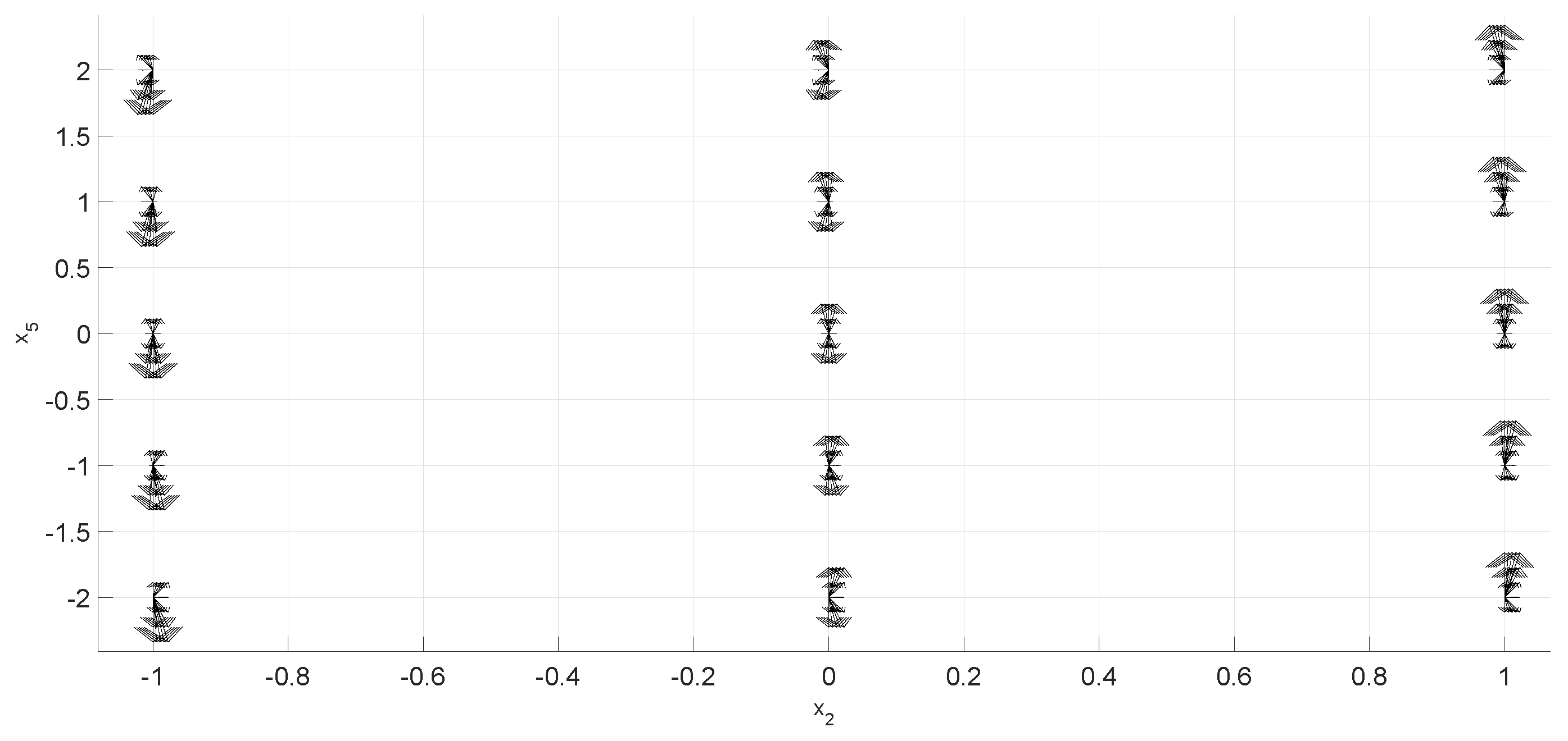
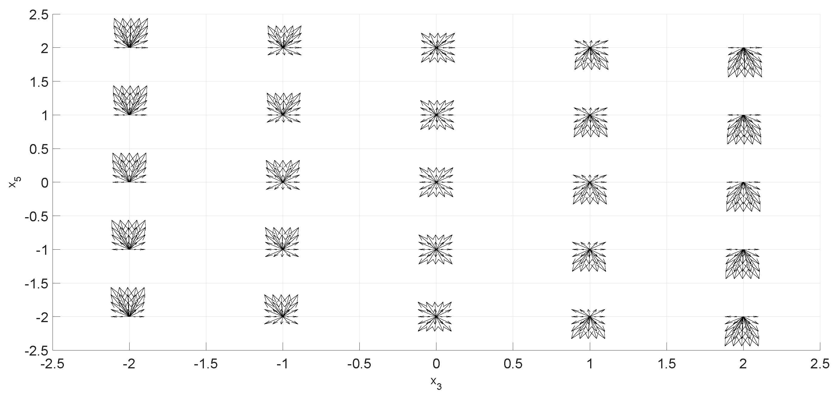
2. The n-Dimensional Phase Portraits by State Combinations
2.1. Foundation
2.2. Procedure
- 1.
- Construct the state space representation of the system.
- 2.
- Define regular initial conditions’ values for each state ().
- 3.
- Construct a phase portrait for each combination of states, a total of.
- 4.
- If necessary, redefine the initial conditions’ values and repeat step 3; that is, get enough sharpness.
- 5.
- Analyze each phase portrait separately.
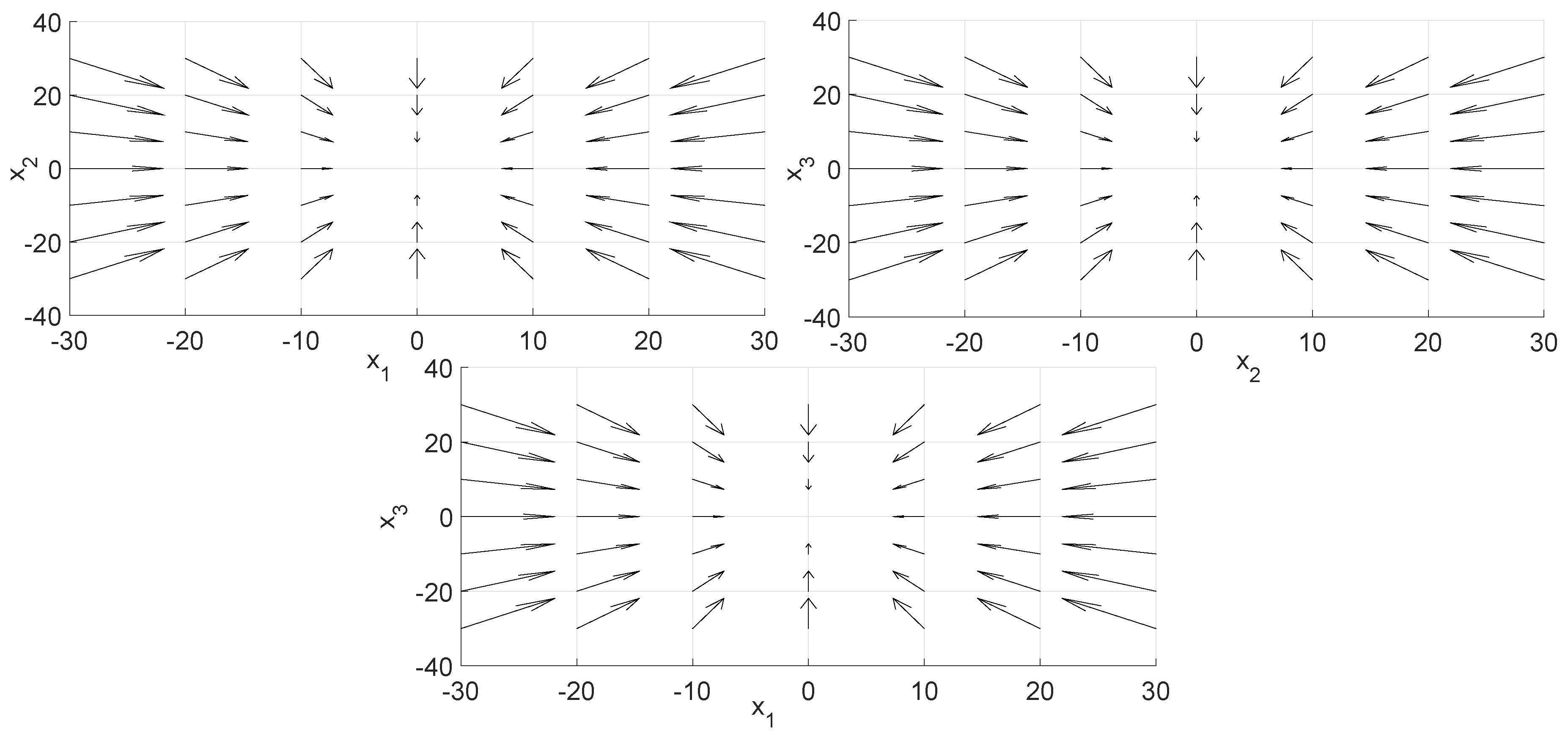
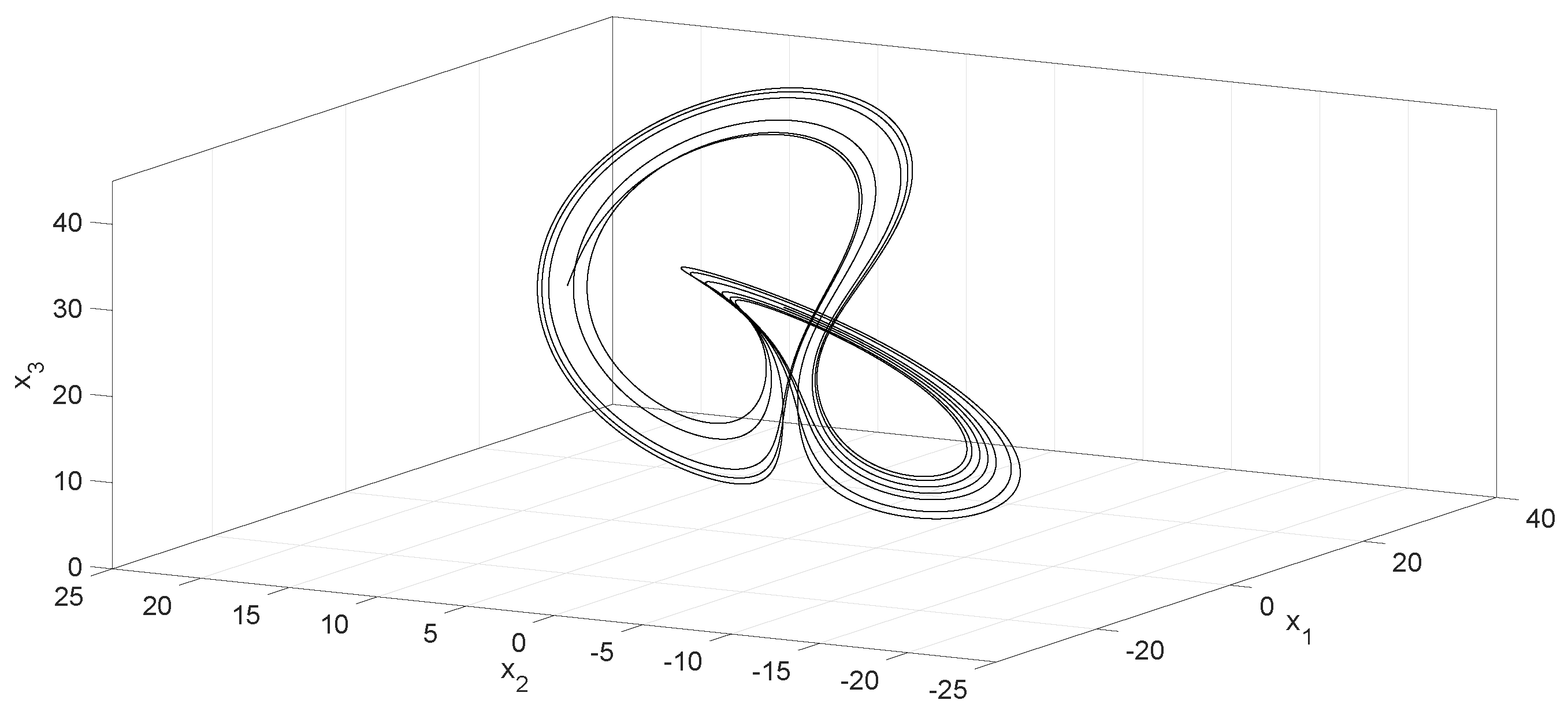
2.3. Examples
| −30 | −30 | −30 |
| −30 | −30 | −20 |
| −30 | −20 | −30 |
| −30 | −20 | −20 |
| ⋮ | ⋮ | ⋮ |
| 30 | 30 | 20 |
| 30 | 30 | 30 |
| , | , | , | ||||||
| −30 | −30 | −30 | 30 | 30 | 30 | 42.4 | 42.4 | 42.4 |
| −30 | −30 | −20 | 30 | 30 | 20 | 42.4 | 36 | 36 |
| −30 | −20 | −30 | 30 | 20 | 30 | 36 | 42.4 | 42.4 |
| −30 | −20 | −20 | 30 | 20 | 20 | 36 | 36 | 28.3 |
| ⋮ | ⋮ | ⋮ | ⋮ | ⋮ | ⋮ | ⋮ | ⋮ | ⋮ |
| 30 | 30 | 20 | −30 | −30 | −20 | 42.4 | 36 | 36 |
| 30 | 30 | 30 | −30 | −30 | −30 | 42.4 | 42.4 | 42.4 |
3. The n-Dimensional Phase Portraits by Coordinates’ Transformations
3.1. Foundation
3.2. Procedure
- 1.
- Construct the state space representation of the system.
- 2.
- Define regular initial conditions values for each state.
- 3
- Linearize if necessary, in every combination of regular initial conditions; alternatively linearize only in an equilibrium point of interest.
- 4.
- Try to found matrices such that; if not possible use another method for order reduction.
- 5.
- Determine the dominant states and construct a phase portrait for each combination of them.
- 6.
- If necessary, redefine the initial conditions values and repeat from step 3; that is, get enough sharpness.
- 7.
- Analyze each phase portrait separately.
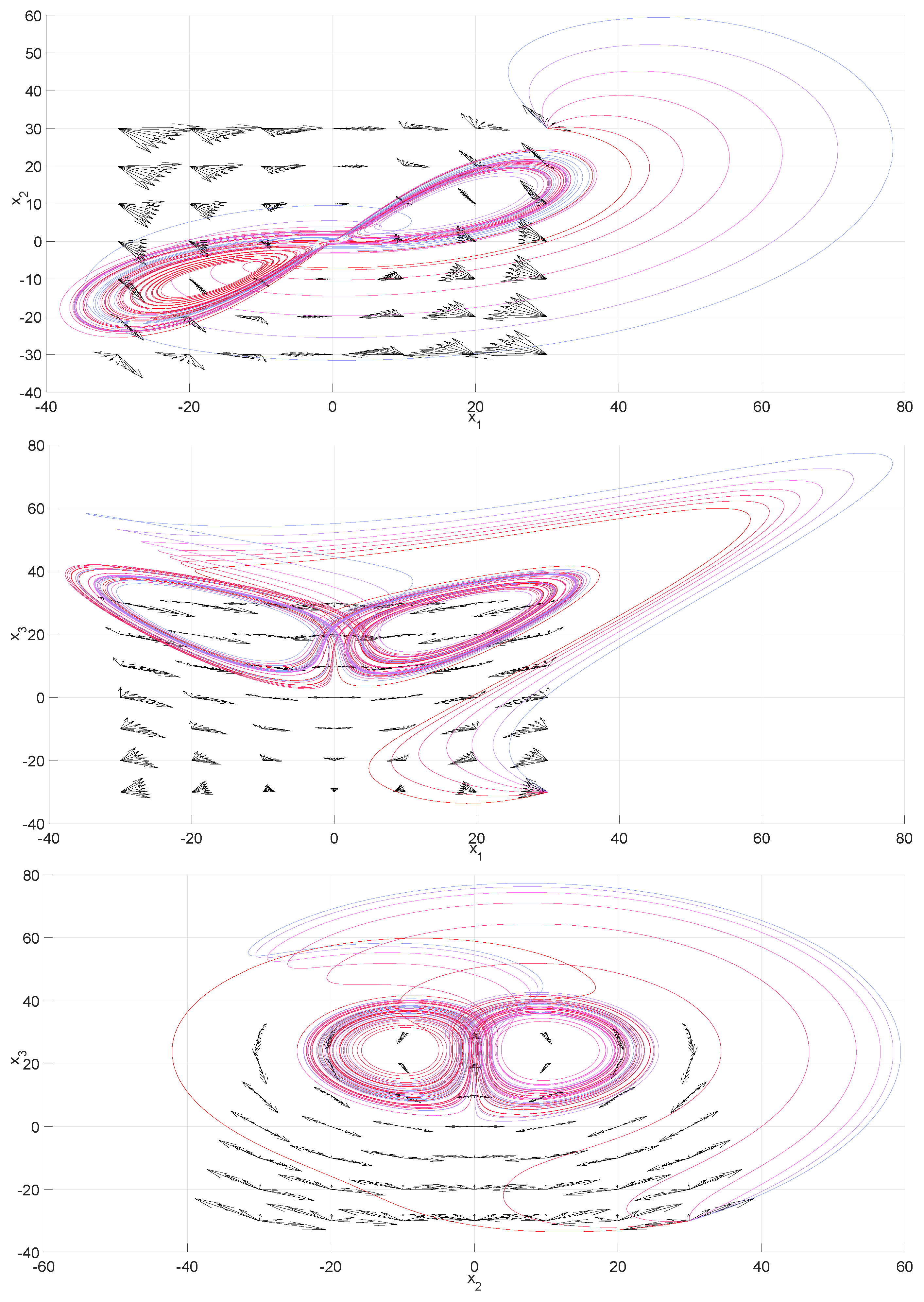
3.3. Examples
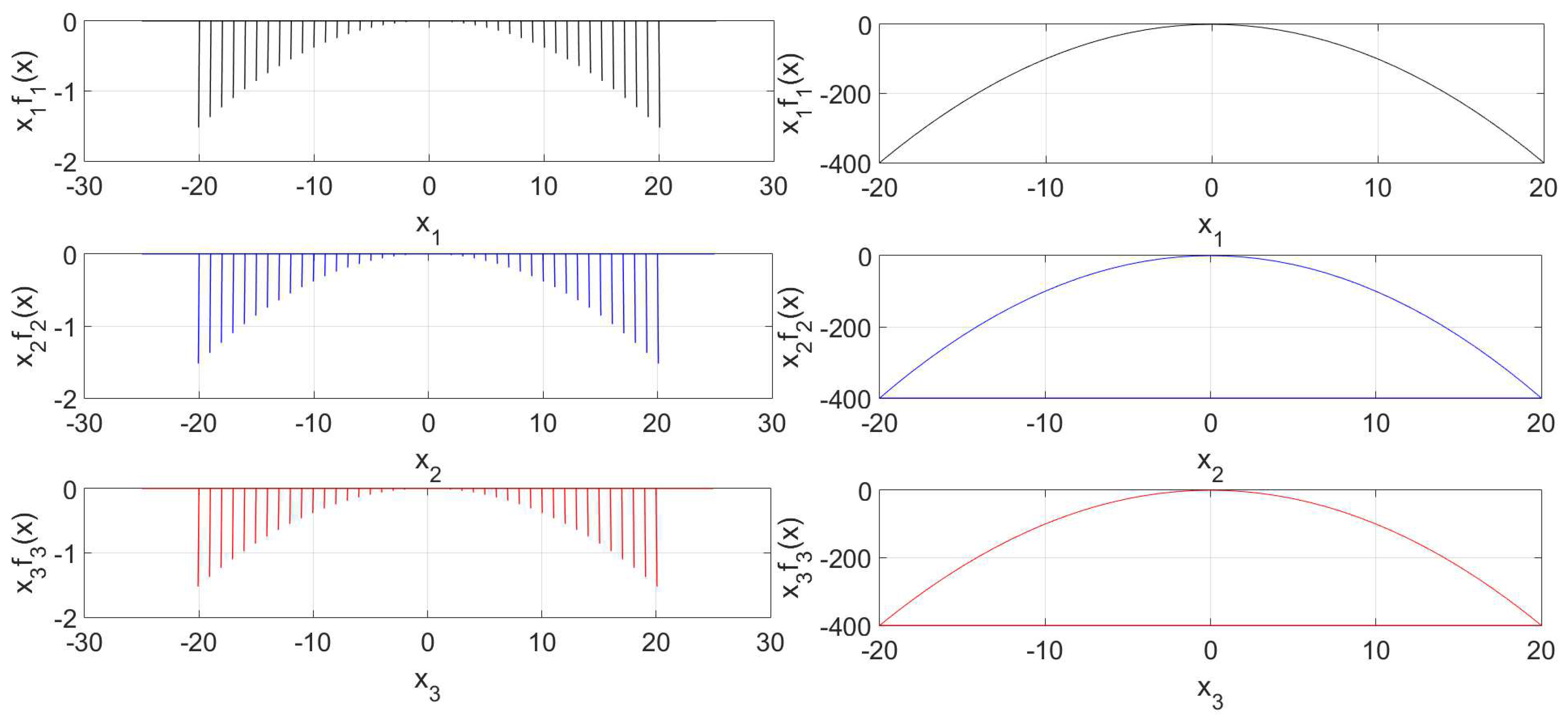
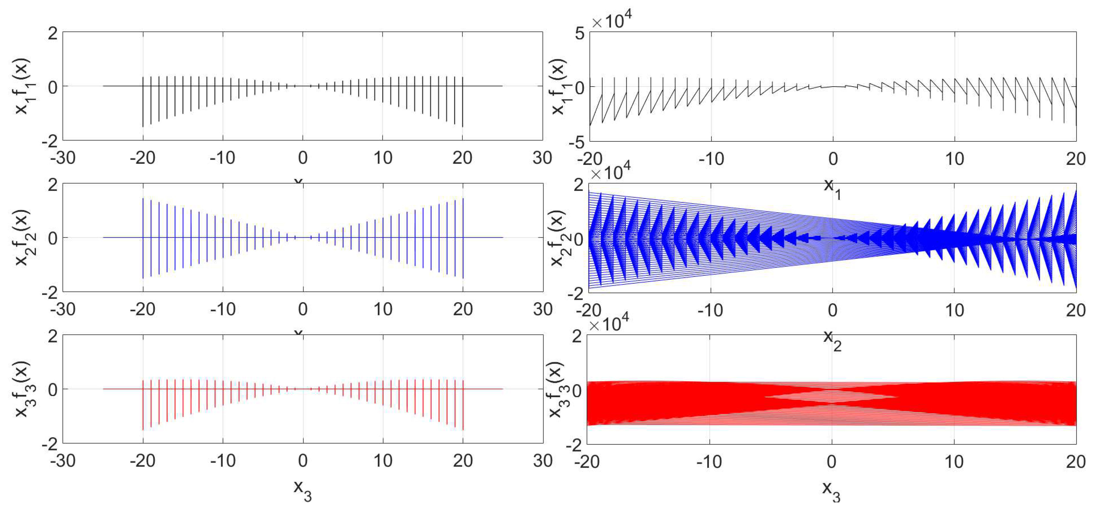
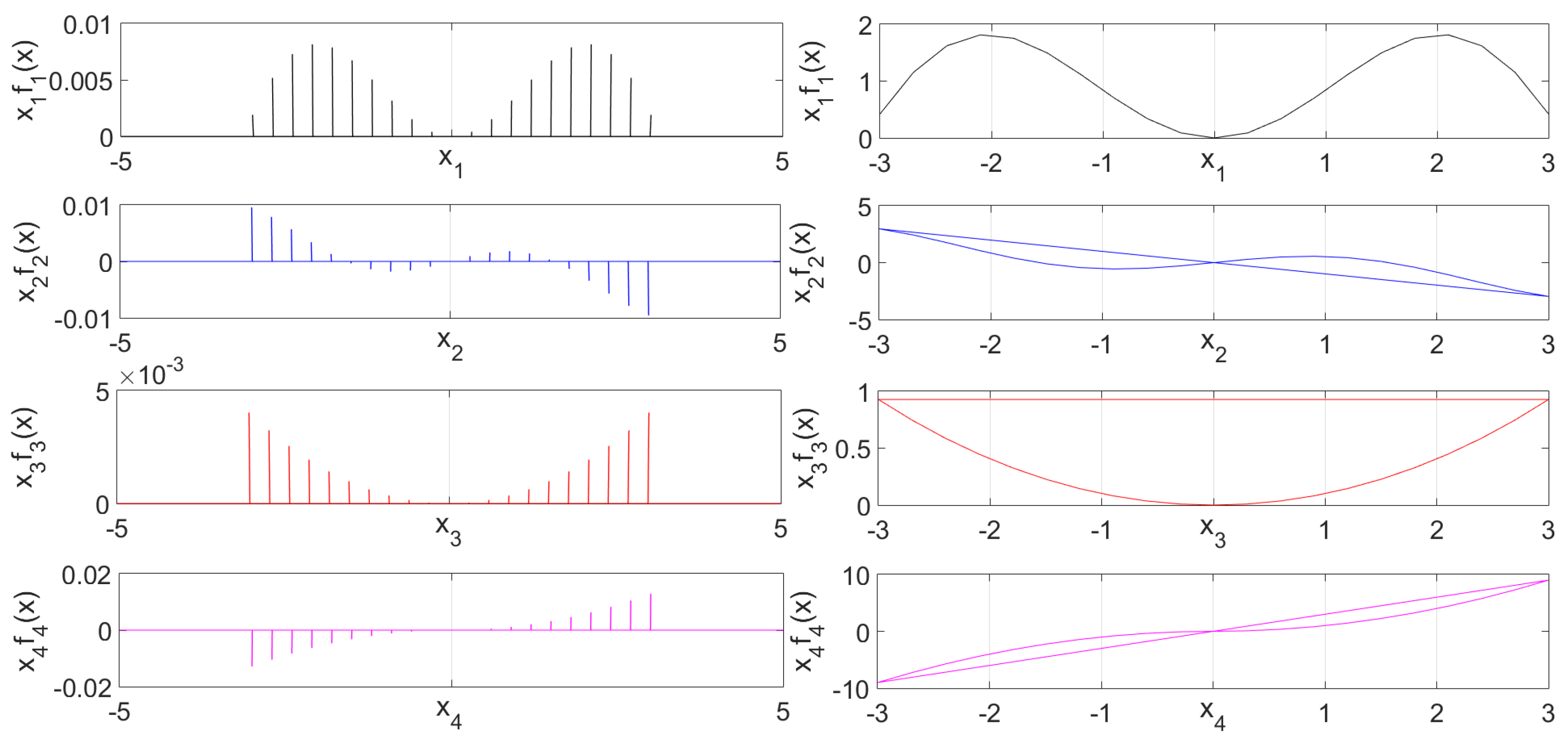
4. The State-by-State n-Dimensional Phase Portraits
4.1. Foundation
4.2. Procedure
- 1.
- Construct the state space representation of the system.
- 2.
- Define regular initial conditions values for each state.
- 3.
- Calculatefor each i-th state, and for the set of initial conditions.
- 4.
- Plot
- 5.
- Repeat Step 3 for each state, a total of n.
- 6.
- If necessary, redefine the initial conditions’ values and repeat from step 5; that is, get enough sharpness.
- 7.
- Analyze each phase portrait separately.
4.3. Examples
5. Conclusions
Author Contributions
Funding
Conflicts of Interest
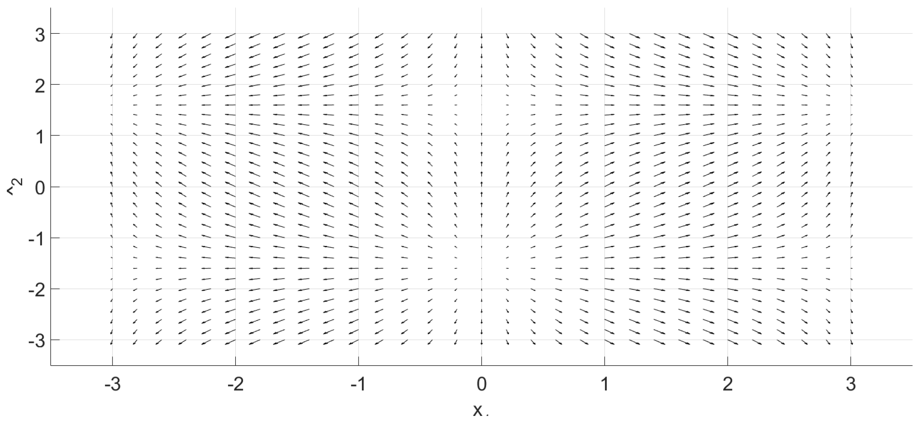
Appendix A. Matlab Code to Generate a n-Dimensional Phase Portrait by State Combinations
- %%%%%%%%%%%%%%%%% Quiver scale %%%%%%%%%%%%%%%%%%%%%%%%%%%%%%%%%
- scale=15;
- %%%%%%%%%%%%%%%%% Generate grid %%%%%%%%%%%%%%%%%%%%%%%%%%%%%%%%
- x=permn(-3:3/15:3,4); %(c) Jos van der Geest library from Matlab
- %%%%%%%%%%%%%%%%% THIS IS THE DYNAMICS %%%%%%%%%%%%%%%%%%%%%%%%%
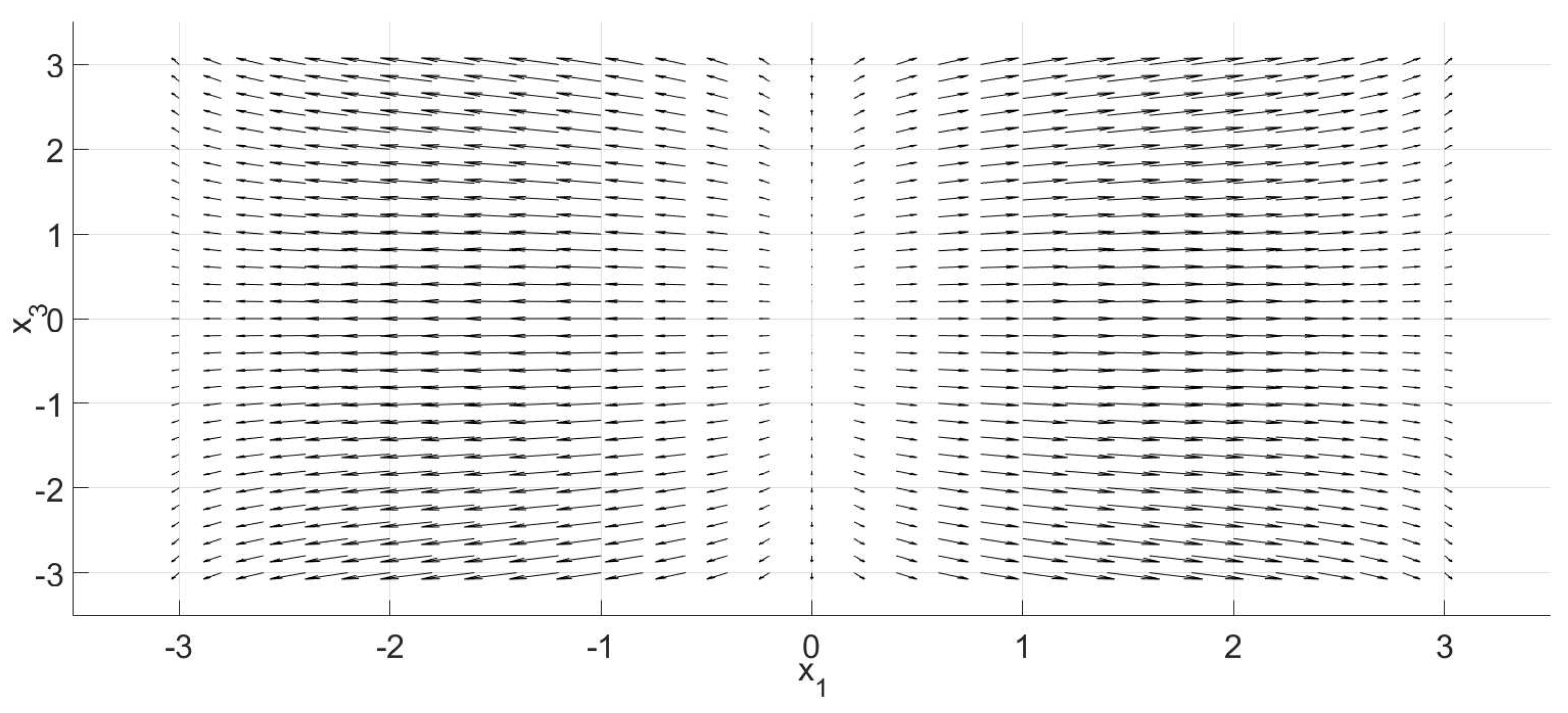
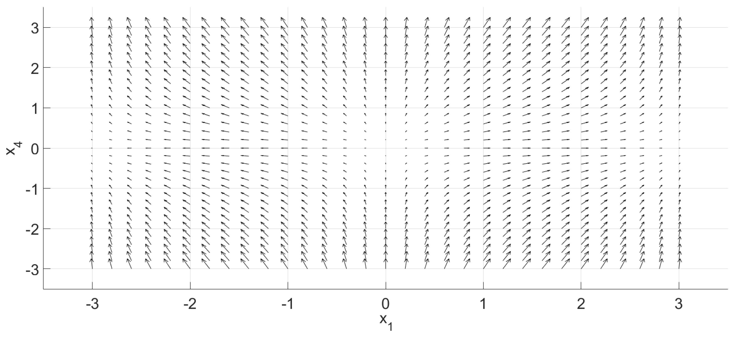
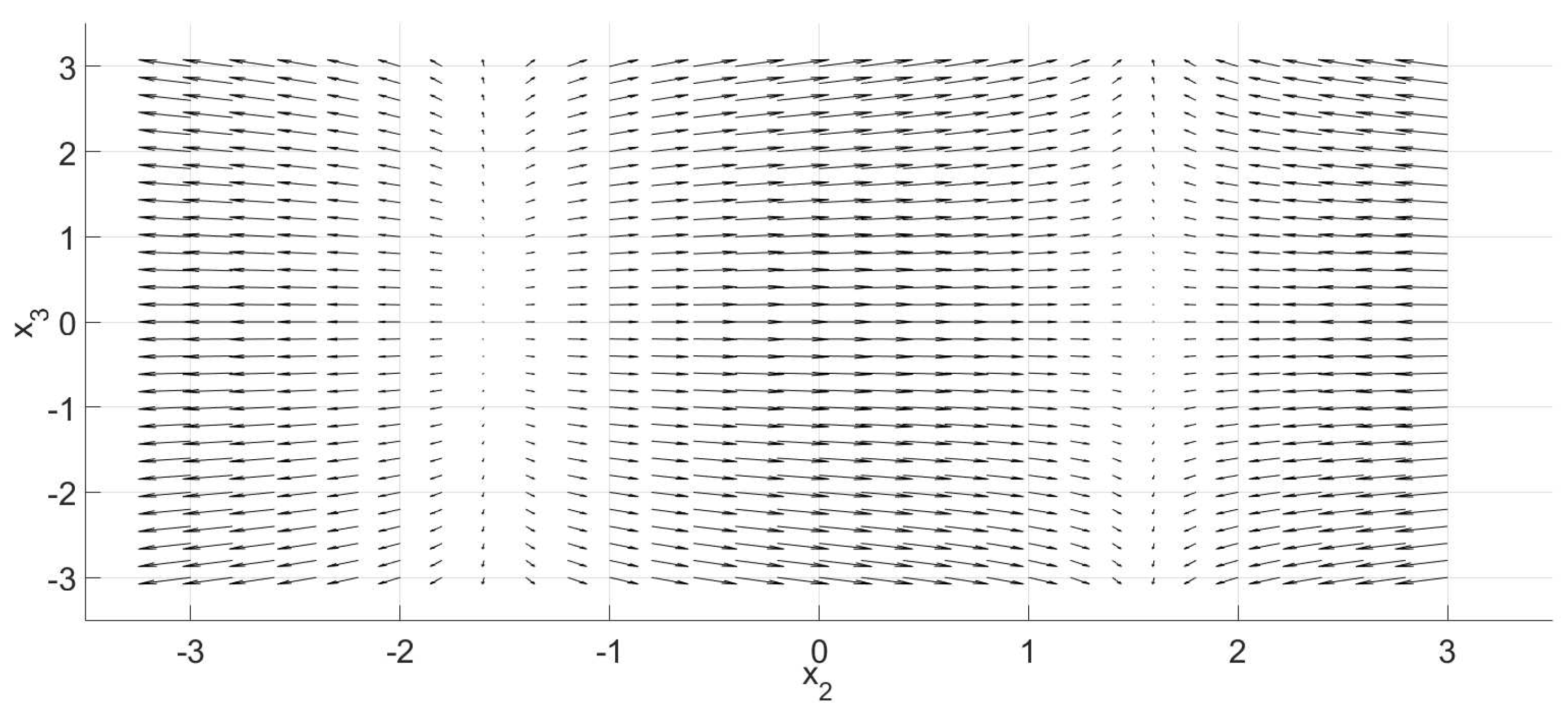
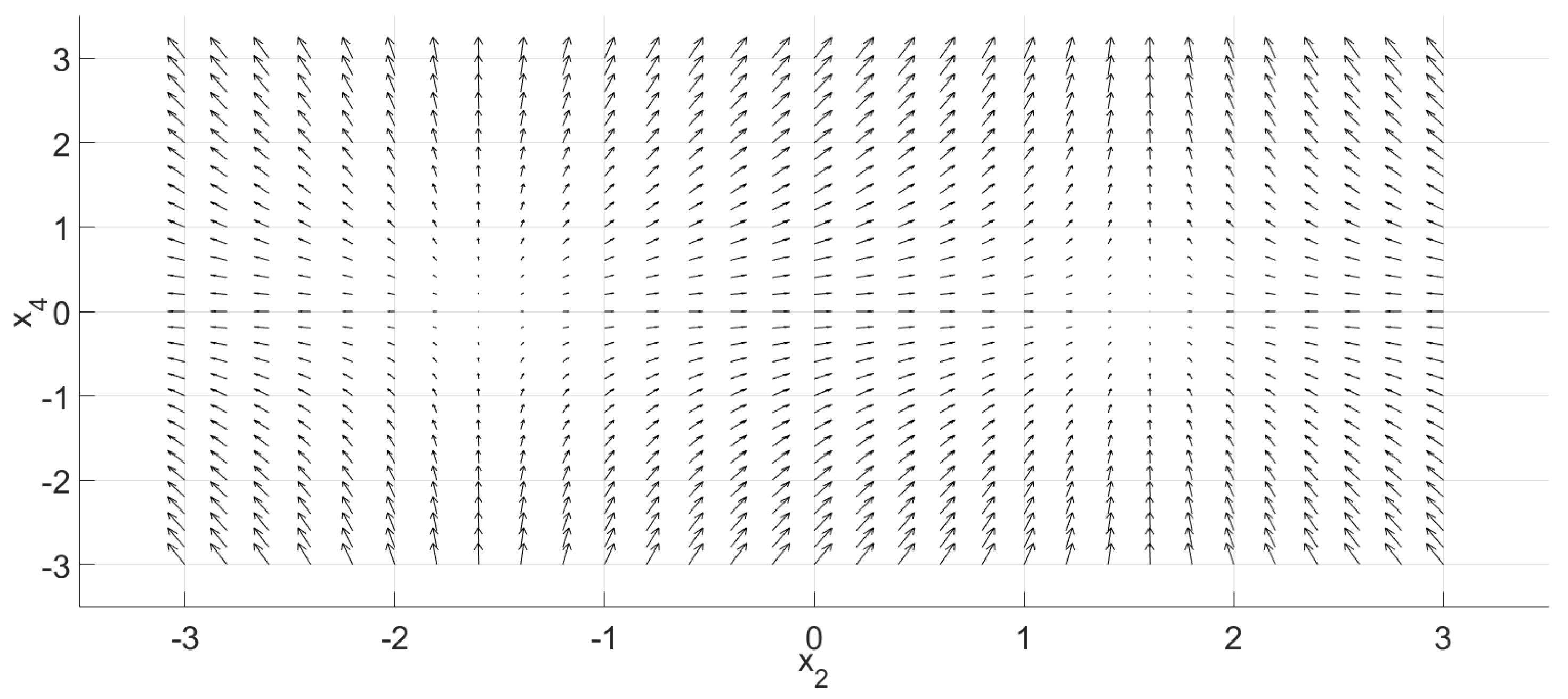
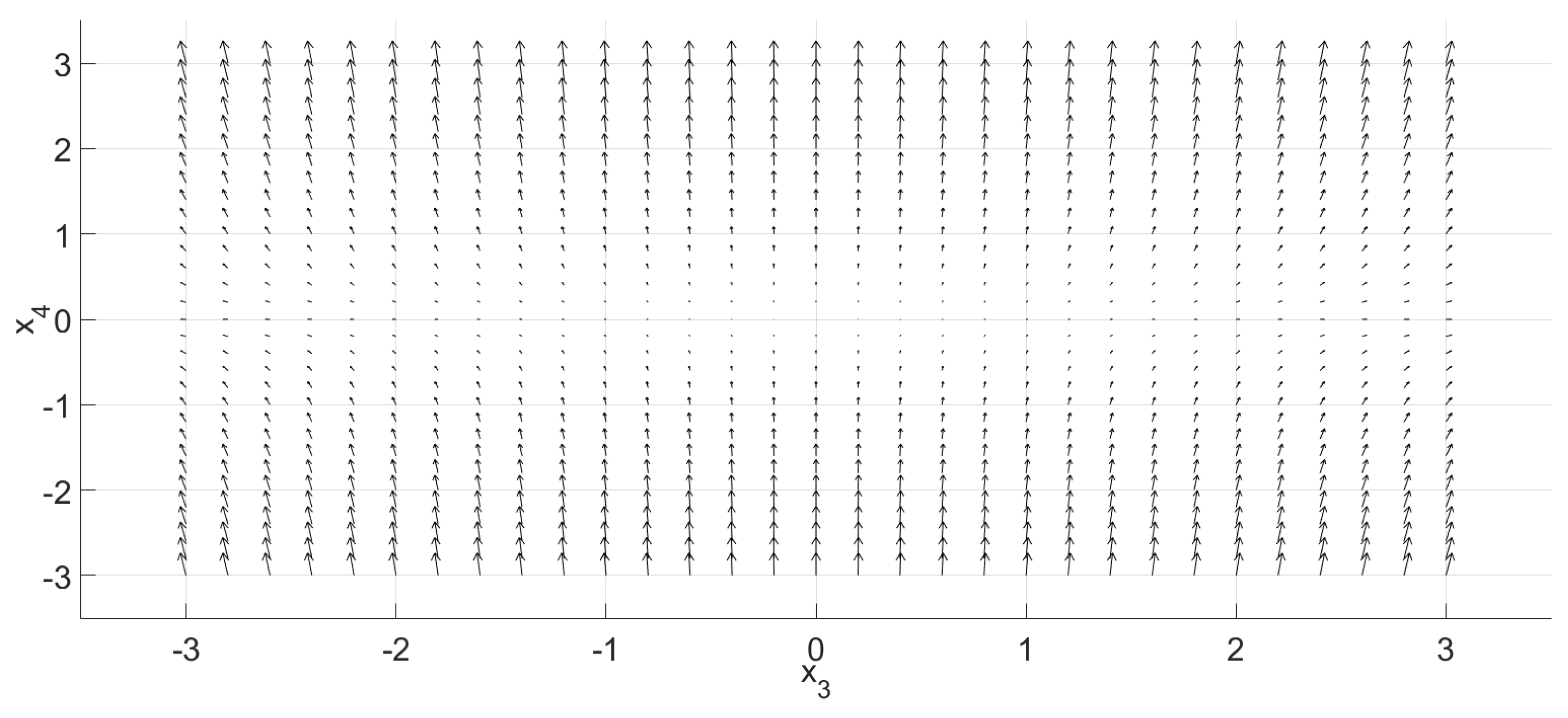
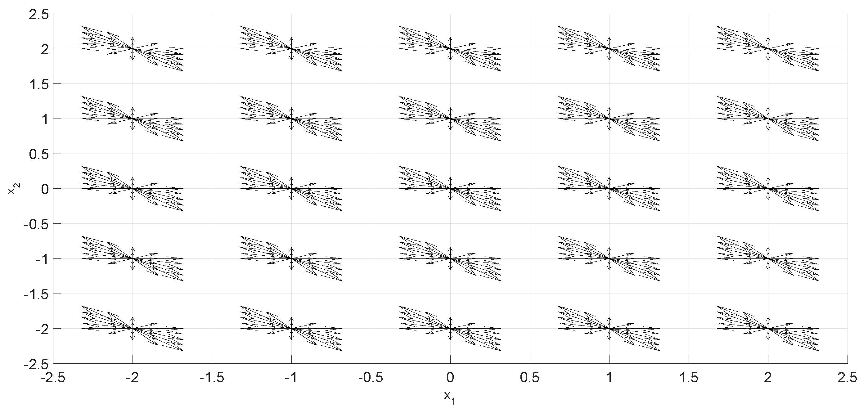
- f=[sin(x(:,1)),cos(x(:,2)),tan(x(:,3)/10),abs(x(:,4))];
- %%%%%%%%%%%%%%%%%%%%%%%%%%%%%%%%%%%%%%%%%%%%%%%%%%%%%%%%%%%%%%%%
- close all
- figure(’Name’,’Phase Portrait x_1 x_2’,’NumberTitle’,’off’)
- hold on
- quiver(x(:,1),x(:,2),f(:,1),f(:,2),scale,’k’)
- xlabel(’x_1’,’FontSize’,18)
- ylabel(’x_2’,’FontSize’,18)
- grid on
- figure(’Name’,’Phase Portrait x_1 x_3’,’NumberTitle’,’off’)
- hold on
- scale=30;
- quiver(x(:,1),x(:,3),f(:,1),f(:,3),scale,’k’)
- xlabel(’x_1’,’FontSize’,18)
- ylabel(’x_3’,’FontSize’,18)
- grid on
- figure(’Name’,’Phase Portrait x_1 x_4’,’NumberTitle’,’off’)
- hold on
- scale=30;
- quiver(x(:,1),x(:,4),f(:,1),f(:,4),scale,’k’)
- xlabel(’x_1’,’FontSize’,18)
- ylabel(’x_4’,’FontSize’,18)
- grid on
- figure(’Name’,’Phase Portrait x_2 x_3’,’NumberTitle’,’off’)
- hold on
- scale=30;
- quiver(x(:,2),x(:,3),f(:,2),f(:,3),scale,’k’)
- xlabel(’x_2’,’FontSize’,18)
- ylabel(’x_3’,’FontSize’,18)
- grid on
- figure(’Name’,’Phase Portrait x_2 x_4’,’NumberTitle’,’off’)
- hold on
- scale=30;
- quiver(x(:,2),x(:,4),f(:,2),f(:,4),scale,’k’)
- xlabel(’x_2’,’FontSize’,18)
- ylabel(’x_4’,’FontSize’,18)
- grid on
- figure(’Name’,’Phase Portrait x_3 x_4’,’NumberTitle’,’off’)
- hold on
- scale=30;
- quiver(x(:,3),x(:,4),f(:,3),f(:,4),scale,’k’)
- xlabel(’x_3’,’FontSize’,18)
- ylabel(’x_4’,’FontSize’,18)
- grid on
- shg
Appendix B. Matlab Code to Generate a State by State n-Dimensional Phase Portrait
- %%%%%%%%%%%%%%%%% Quiver scale %%%%%%%%%%%%%%%%%%%%%%%%%%%%%%%%%
- scale=1;
- %%%%%%%%%%%%%%%%% Generate grid %%%%%%%%%%%%%%%%%%%%%%%%%%%%%%%%
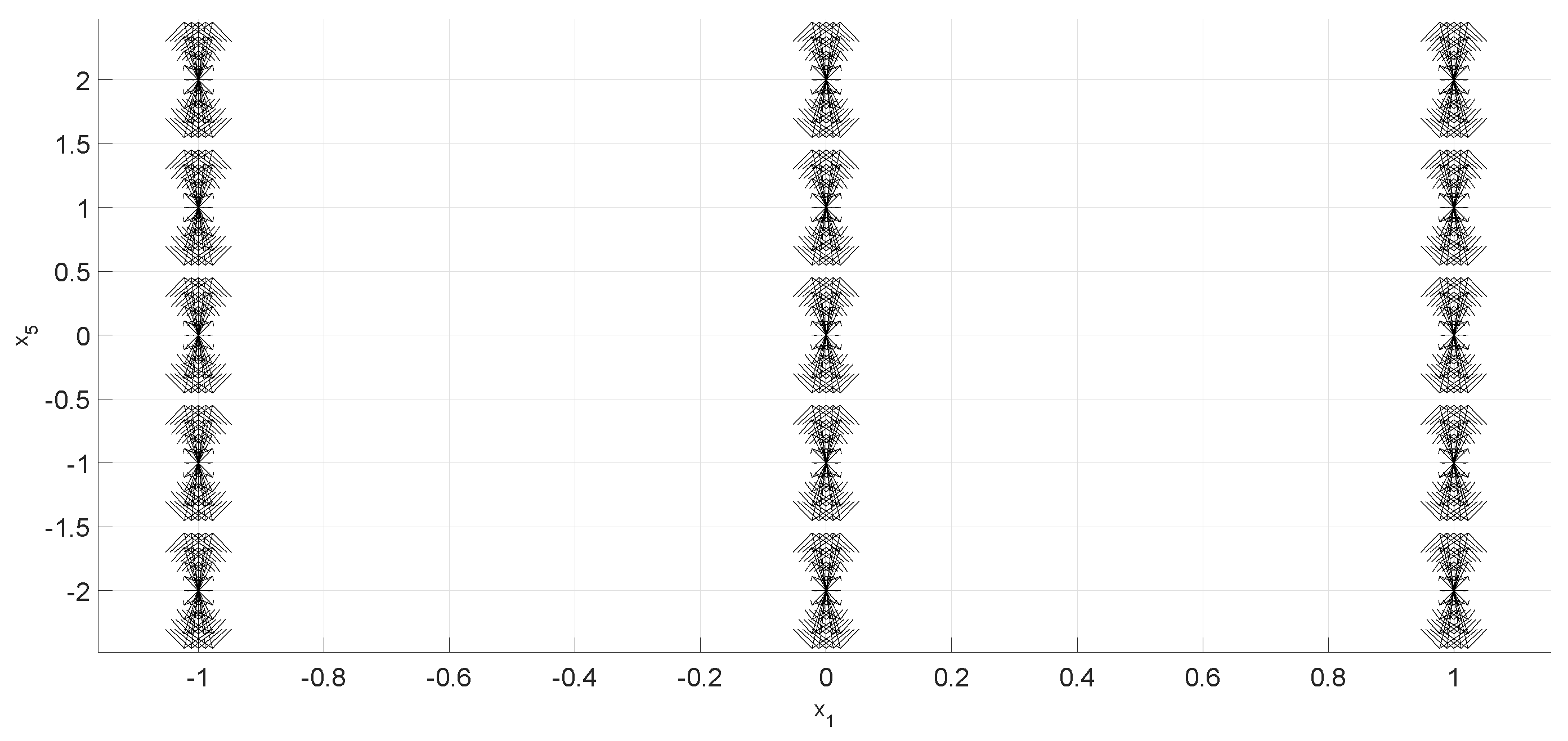
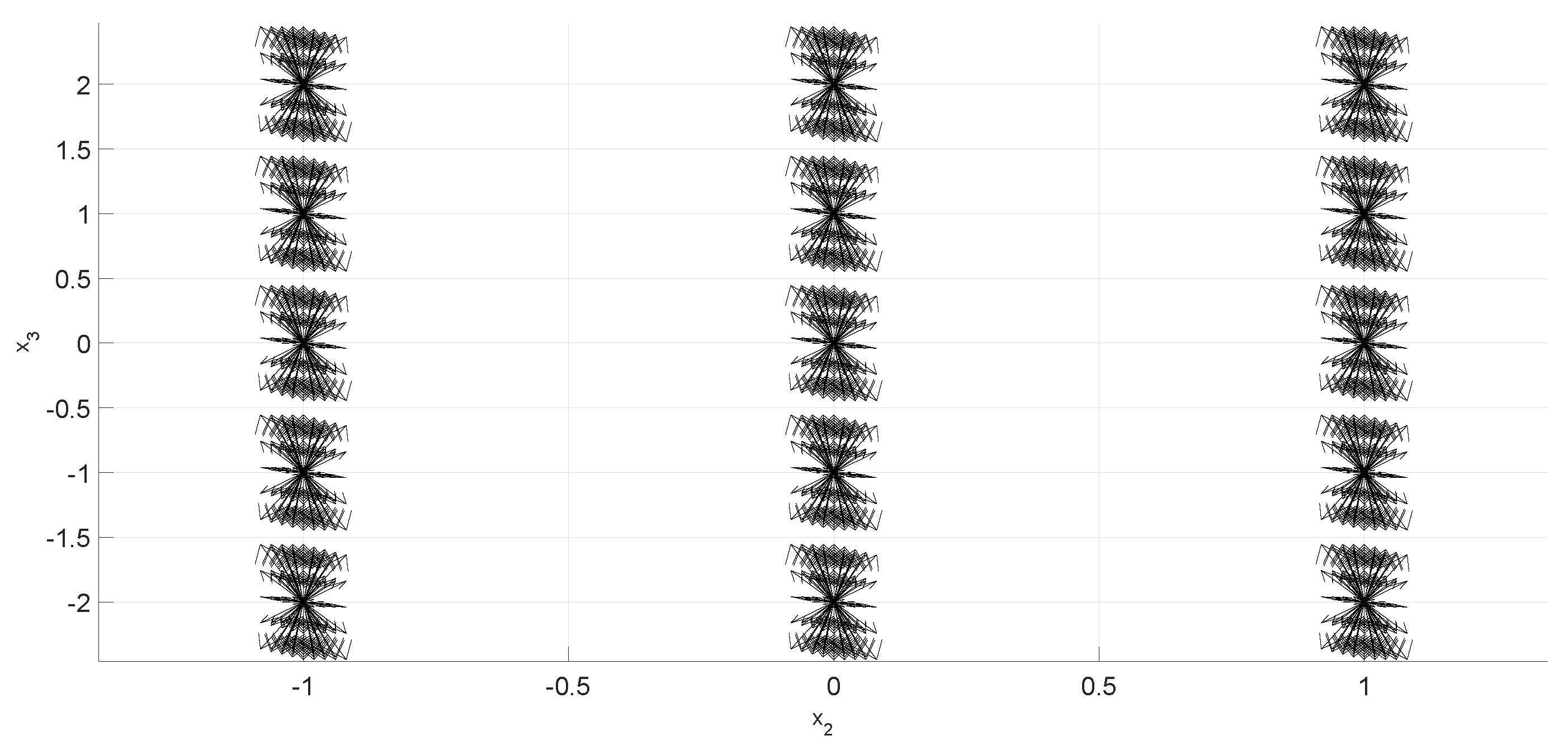
- x=permn(-3:3/10:3,4); %(c) Jos van der Geest library from Matlab
- %%%%%%%%%%%%%%%%% THIS IS THE DYNAMICS %%%%%%%%%%%%%%%%%%%%%%%%%
- f=[sin(x(:,1)),cos(x(:,2)),tan(x(:,3)/10),abs(x(:,4))];
- %%%%%%%%%%%%%%%%%%%%%%%%%%%%%%%%%%%%%%%%%%%%%%%%%%%%%%%%%%%%%%%%
- s=size(x(:,1));
- vy=zeros(s(:,1),1);
- z=1:1:s(:,1);
- z=z’;
- close all
- subplot(4,1,1)
- quiver( x(:,1) , y , x(:,1) , x(:,1).∗f(:,1) ,scale,’k’,’ShowArrowHead’,
- ’off’,’MaxHeadSize’,0.05,’AlignVertexCenters’,’on’,’LineWidth’,1)
- hold on;
- line([-5 5],[0 0],’Color’,’k’)
- subplot(4,1,2)
- quiver( x(:,2) , y , x(:,2) , x(:,2).∗f(:,2) ,scale,’b’,’ShowArrowHead’,
- ’off’,’MaxHeadSize’,0.05,’AlignVertexCenters’,’on’,’LineWidth’,1)
- hold on;
- line([-5 5],[0 0],’Color’,’b’)
- subplot(4,1,3)
- quiver( x(:,3) , y , x(:,3) , x(:,3).∗f(:,3) ,scale,’r’,’ShowArrowHead’,
- ’off’,’MaxHeadSize’,0.05,’AlignVertexCenters’,’on’,’LineWidth’,1)
- hold on;
- line([-5 5],[0 0],’Color’,’r’)
- subplot(4,1,4)
- quiver( x(:,4) , y , x(:,4) , x(:,4).∗f(:,4) ,scale,’m’,’ShowArrowHead’,
- ’off’,’MaxHeadSize’,0.05,’AlignVertexCenters’,’on’,’LineWidth’,1)
- hold on;
- line([-5 5],[0 0],’Color’,’m’)
- figure
- vsubplot(4,1,1)
- vplot(x(:,1),x(:,1).∗f(:,1),’k’)
- subplot(4,1,2)
- plot(x(:,2),x(:,2).∗f(:,2),’b’)
- subplot(4,1,3)
- plot(x(:,3),x(:,3).∗f(:,3),’r’)
- subplot(4,1,4)
- plot(x(:,4),x(:,4).∗f(:,4),’m’)
References
- Ifrah, G.; Harding, E.F.; Bellos, D.; Wood, S.; Harding, E.F. The Universal History of Computing: From the Abacus to Quantum Computing; John Wiley & Sons, Inc.: New York, NY, USA, 2000. [Google Scholar]
- Dorf, R.C.; Bishop, R.H. Modern Control Systems; Pearson: New York, NY, USA, 2011. [Google Scholar]
- Mermoud, G. Stochastic Reactive Distributed Robotic Systems; Springer: New York, NY, USA, 2014. [Google Scholar]
- Teschl, G. Ordinary Differential Equations and Dynamical Systems; American Mathematical Society: Ann Arbor, MI, USA, 2012; Volume 140. [Google Scholar]
- Khalil, H.K. Nonlinear Control; Pearson: New York, NY, USA, 2015. [Google Scholar]
- Xiong, L.; Liu, Z.; Zhang, X. Analysis, circuit implementation and applications of a novel chaotic system. Circuit World 2017, 43, 118–130. [Google Scholar] [CrossRef]
- Ahmad, I.; Saaban, A.B.; Ibrahim, A.B.; Shahzad, M. A research on active control to synchronize a new 3D chaotic system. Systems 2016, 4, 2. [Google Scholar] [CrossRef]
- Ge, G.; Wang, W. The application of the undetermined fundamental frequency method on the period-doubling bifurcation of the 3D nonlinear system. In Abstract and Applied Analysis; Hindawi: New York, NY, USA, 2013; Volume 2013. [Google Scholar]
- Rocha, R.; Andrucioli, G.L.; Medrano-T, R.O. Experimental characterization of nonlinear systems: A real-time evaluation of the analogous Chua’s circuit behavior. Nonlinear Dyn. 2010, 62, 237–251. [Google Scholar] [CrossRef]
- Deekshatulu, B. The x n-x plane for analysis of certain second-order nonlinear systems. IEEE Trans. Appl. Ind. 1963, 82, 315–317. [Google Scholar] [CrossRef]
- Shlomo, S.; Prakash, M. Phase space distribution of an N-dimensional harmonic oscillator. Nucl. Phys. A 1981, 357, 157–170. [Google Scholar] [CrossRef]
- Wilson-Jones, R.; Wellstead, P. A generalised phase portrait for piecewise linear system analysis. In Proceedings of the International Conference on Control IET, Coventry, UK, 21–24 March 1994; Volume 1, pp. 85–88. [Google Scholar]
- Zhao, F. Extracting and representing qualitative behaviors of complex systems in phase space. Artif. Intell. 1994, 69, 51–92. [Google Scholar] [CrossRef]
- Pettit, N.B.; Wellstead, P.E. Analyzing piecewise linear dynamical systems. IEEE Control Syst. 1995, 15, 43–50. [Google Scholar]
- Elhadj, Z.; Sprott, J. Some explicit formulas of Lyapunov exponents for three-dimensional quadratic mappings. Front. Phys. China 2009, 4, 549–555. [Google Scholar] [CrossRef]
- Volos, C.; Maaita, J.O.; Vaidyanathan, S.; Pham, V.T.; Stouboulos, I.; Kyprianidis, I. A novel 4-D hyperchaotic four-wing system with a saddle-focus equilibrium. IEEE Trans. Circuits Syst. II Express Briefs 2016, 64, 339–343. [Google Scholar] [CrossRef]
- Qi, G.; Chen, G.; Du, S.; Chen, Z.; Yuan, Z. Analysis of a new chaotic system. Phys. A Stat. Mech. Appl. 2005, 352, 295–308. [Google Scholar] [CrossRef]
- Schilders, W.H.; Van der Vorst, H.A.; Rommes, J. Model Order Reduction: Theory, Research Aspects and Applications; Springer: New York, NY, USA, 2008; Volume 13. [Google Scholar]
- Armaou, A.; Christofides, P.D. Dynamic optimization of dissipative PDE systems using nonlinear order reduction. Chem. Eng. Sci. 2002, 57, 5083–5114. [Google Scholar] [CrossRef]
- Amsallem, D.; Zahr, M.J.; Farhat, C. Nonlinear model order reduction based on local reduced-order bases. Int. J. Numer. Methods Eng. 2012, 92, 891–916. [Google Scholar] [CrossRef]
- Nayfeh, A.H. Order reduction of retarded nonlinear systems—The method of multiple scales versus center-manifold reduction. Nonlinear Dyn. 2008, 51, 483–500. [Google Scholar] [CrossRef]
- Kerschen, G.; Golinval, J.C.; Vakakis, A.F.; Bergman, L.A. The method of proper orthogonal decomposition for dynamical characterization and order reduction of mechanical systems: An overview. Nonlinear Dyn. 2005, 41, 147–169. [Google Scholar] [CrossRef]
- Pillage, L.T.; Rohrer, R.A. Asymptotic waveform evaluation for timing analysis. IEEE Trans. Comput.-Aided Des. Integr. Circuits Syst. 1990, 9, 352–366. [Google Scholar] [CrossRef]
- Deo, N. Graph Theory with Applications to Engineering and Computer Science; Courier Dover Publications: New York, NY, USA, 2017. [Google Scholar]
- Saad, Y. Iterative Methods for Sparse Linear Systems; SIAM: Philadelphia, PA, USA, 2003; Volume 82. [Google Scholar]
- Odabasioglu, A.; Celik, M.; Pileggi, L.T. PRIMA: Passive reduced-order interconnect macromodeling algorithm. In Proceedings of the 1997 IEEE/ACM International Conference on Computer-Aided Design, San Jose, CA, USA, 1 May 1997; IEEE Computer Society: Washington, DC, USA, 1997; pp. 58–65. [Google Scholar]
- Chen, Y.; White, J.; Macromodeling, T. A quadratic method for nonlinear model order reduction. In Proceedings of the 2000 International Conference on Modeling and Simulation of Microsystems, San Jose, CA, USA, 27–29 March 2000; pp. 477–480. [Google Scholar]
- Benner, P.; Mehrmann, V.; Sorensen, D.C. Dimension Reduction of Large-Scale Systems; Springer: New York, NY, USA, 2005; Volume 35. [Google Scholar]
- Antoulas, A.C. Approximation of Large-Scale Dynamical Systems; SIAM: Philadelphia, PA, USA, 2005; Volume 6. [Google Scholar]
- Morales-Saldana, J.; Gutierrez, E.C.; Leyva-Ramos, J. Modeling of switch-mode DC-DC cascade converters. IEEE Trans. Aerosp. Electron. Syst. 2002, 38, 295–299. [Google Scholar] [CrossRef]


© 2019 by the authors. Licensee MDPI, Basel, Switzerland. This article is an open access article distributed under the terms and conditions of the Creative Commons Attribution (CC BY) license (http://creativecommons.org/licenses/by/4.0/).
Share and Cite
Rodríguez-Licea, M.-A.; Perez-Pinal, F.-J.; Nuñez-Pérez, J.-C.; Sandoval-Ibarra, Y. On the n-Dimensional Phase Portraits. Appl. Sci. 2019, 9, 872. https://doi.org/10.3390/app9050872
Rodríguez-Licea M-A, Perez-Pinal F-J, Nuñez-Pérez J-C, Sandoval-Ibarra Y. On the n-Dimensional Phase Portraits. Applied Sciences. 2019; 9(5):872. https://doi.org/10.3390/app9050872
Chicago/Turabian StyleRodríguez-Licea, Martín-Antonio, Francisco-J. Perez-Pinal, José-Cruz Nuñez-Pérez, and Yuma Sandoval-Ibarra. 2019. "On the n-Dimensional Phase Portraits" Applied Sciences 9, no. 5: 872. https://doi.org/10.3390/app9050872
APA StyleRodríguez-Licea, M.-A., Perez-Pinal, F.-J., Nuñez-Pérez, J.-C., & Sandoval-Ibarra, Y. (2019). On the n-Dimensional Phase Portraits. Applied Sciences, 9(5), 872. https://doi.org/10.3390/app9050872