Abstract
Manufacturing companies usually expect strategic improvements to focus on reducing both waste and variability in processes, whereas markets demand greater flexibility and low product costs. To deal with this issue, lean manufacturing (LM) emerged as a solution; however, it is often challenging to evaluate its true effect on corporate performance. This challenge can be overcome, nonetheless, by treating it as a multi-criteria problem using the Hesitant Fuzzy linguistic and Technique for Order Preference by Similarity to Ideal Solution (TOPSIS) method. In fact, the hesitant fuzzy linguistic term sets (HFLTS) is vastly employed in decision-making problems. The main contribution of this work is a method to assess the performance of LM applications in the manufacturing industry using the hesitant fuzzy set and TOPSIS to deal with criteria and attitudes from decision makers regarding such LM applications. At the end of the paper, we present a reasonable study to analyze the obtained results.
1. Introduction
Lean manufacturing (LM) combines a wide rage of management practices, such as just in time (JIT), quality systems, work teams, cellular manufacturing, and supply chain management (SCM) in a whole system [1]. The LM method aims at saving costs by reducing waste in the manufacturing system, thereby dealing with economic aspects [2]. Nowadays, LM covers the multiple stages of a product’s life cycle, from its development and manufacturing to its delivery [3]; however, LM is also a challenge amid mass production practices, especially as quality products, and customer satisfaction are prioritized, inventory, time to market and manufacturing space, and everything that adds no value to a product is systematically categorized as waste [4]. LM is often discussed with respect to key performance indicators (KPIs) [5,6]. In addition, Kan et al. [7] affirm the KPI parameters have an association with LM performance. In fact, research evidence has found that LM practices have a positive impact on operational performance [8,9], yet it is often challenging to assess company performance with respect to LM implementation [10,11] and, according to [12,13], it is an attractive and hot topic for exploration through multi-criteria decision-making (MCDM) methodologies.
MCDM has recently gained relevance, especially in engineering [14,15]; however, when an MCDM problem involves objective and subjective information, experts discuss the classical hybrid MCDM method with the fuzzy sets theory [16,17]. In this sense, motivated by the hesitant fuzzy set, Rodríguez et al. [18] introduced the hesitant fuzzy linguistic term sets (HFLTS), which allows decision makers to elicit several linguistic terms for the same linguistic variable [17,19]. Nowadays, the HFLTS is a popular effective tool for representing hesitant qualitative judgments from decision makers; consequently, multiple HFLTS-based decision-making methods have been developed [20]. For instance, in their work, Hwang and Yoon [21] introduced the Technique of Order of Preference by Similarity to Ideal Solution (TOPSIS) method. TOPSIS method is denoted like a significant research issue, which has received a prodigious deal of attention from academics [22,23,24,25]. Additionally, there is HFLTS of TOPSIS proposed by [26,27].
The two main contributions of this work can be stated as follows: first, we propose an HFLTS-based data handling procedure to deal with lean manufacturing performance assessments. The procedure can handle KPI matrices of arbitrary preferences in decision-making situations. Second, we propose a systematic solution to measure the LM performance with respect to a series of criteria. The remainder of this paper is organized in five sections. Section 2 introduces a series of basic definitions of HFLTS and TOPSIS, whereas in Section 3 we present materials and methods which describes details about our application. Next, whereas Section 4 presents a numerical example to illustrate our approach to multi-attribute decision making, in Section 5, we describe the result analysis and discussions related to our method. Finally, research conclusions are proposed in Section 6.
2. Preliminaries
This section introduces basic definitions related to HFLTSs and TOPSIS, as they will be necessary to better understand subsequent sections.
2.1. Hesitant Fuzzy Linguistic Term Sets (HFLTSs)
An HFLTS is a very operative and flexible method that emphasizes one explicit type of complex language term, i.e., reasonable linguistic terms. An HFLTS is a successive, ordered, and finite subset of a specified linguistic term set [17].
Definition 1
([28]). Let us assume that is a fixed set of grammar and depict a hesitant linguistic fuzzy set (HLFS) on Z using a function that when applied to Z encompasses a subset of [0,1]. At the same time, per convenience, the description of the grammar will be called . Then, the grammar set is presented, as follows:
Definition 2
([18]). Given an HFLTS as in Equation (2), its envelope, denoted by env, is defined by an uncertain linguistic terms (ULT) [29] whose limits are the upper and lower bounds of , i.e.,
where and , ,
Definition 3
([30]). Assuming that represents a linguistic term set (LTS), HFLTS , is an ordered and finite subset of consecutive linguistic term of .
Definition 4
([31]). The score function is presented as follows:
Definition 5
(Distance [26,28,31,32]). Assuming that and are two HFLTS and env and env
where β represents a higher element from and depicts the maximum or higher element from . Thus, α denotes a low element from and depicts the minimal or low element from :
where ρ depicts # of the elements of the set ς and, stands for the subfix of linguistic term
Definition 6
([30]). Let be a linguistic term set. A hesitant fuzzy linguistic term sets (HFLTS), , is an ordered and finite subset of the consecutive linguistic terms of S.
In addition, an HFLTS can be used to elicit several linguistic values for a linguistic term, yet it is still not comparable to human thinking and reasoning processes. Thus, Rodríguez et al. [18] further presented a context-free grammar to describe linguistic terms that are more parallel to the human expressions and can be simply denoted by means of HFLTSs. In addition, according to [20], the grammar is used to express the linguistic term and transformed to HFLEs by using function :
2.2. TOPSIS in Conventional Version
In this section, the conventional manner of TOPSIS is presented
- Step 1.
- Establish the final decisión matrix.Table 1 shows the set of the alternatives and be a finite set of criteria involved in the MCDM problem.
 Table 1. Final decision matrix.
 - Step 2.
- Normalize the final decision matrix using Equation (6):where
- Step 3.
- Construct the aggregate matrixwhereand represents the weight vector of the criteria
- Step 4.
- Step 5.
- Compute the and
- Step 6.
- Ranking of the alternatives
3. Materials and Methods
This section presents the material and method used in the investigation. We introduce the procedure of HFLTs and TOPSIS for the Lean Improvement Assessment. At the same time, in order to explain the proposed method, Figure 1 shows the flowcharts of the different steps about it.
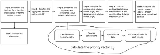
Figure 1.
Flowcharts of the algorithms to assess the Lean Manufacturing Performance.
Hesitant Fuzzy Linguistic Term and TOPSIS to Assess Lean Performance
In this section, we introduce an algorithm through a Hesitant Fuzzy Linguistic Term and TOPSIS in order to be applied to Lean Improvement Assessment. The method is described in the following steps:
- Step 1.
- Determine the hesitant fuzzy decision matrix called = for the MCDM problem. Appraisal the alternative with respect to DM preferences and the criteria.
- Step 2.
- Calculate the aggregated decision matrix called Z. This process requires the aggregation of the preferences of the DMs through Equations (14) and (15).Then, where , ,
- Step 3.
- Determine the importance or preference about criteria called vector , for the MCDM problem via Analytic Hierarchy Process (AHP) method proposed by [33]. Appraise the criteria with respect to DM preferences.
- Step 4.
- Compute the positive-ideal solution vector and Negative-ideal solution vector . At this mode, the evaluation of alternative by mean of criterion is symbolized as using an aggregated matrix Z. Thus, depicts a set of benefit criteria and represents the greater preference of the criterion and depicts a set of cost criteria and describes the smaller preference of the criterion :Then, , ,thus , .
- Step 5.
- Construct positive ideal distance matrix and negative ideal distance matrix , which are denoted as follows:
- Step 6.
- Calculate the relative closeness of each alternative to the ideal solution as follows:whereand
- Step 7.
- Rank all the alternatives
4. Numerical Example
This section introduces a real-life example, which was applied in an automotive company based in Ciudad Juárez, Chihuahua, Mexico. The company works under an LM methodology and focuses on minimizing operational waste; thus, managers are particularly interested in assessing the real impact of the LM methodology. To this end, a group of experts first assessed the company’s LM implementation improvement metrics. Simultaneously, we described the set of criteria and the KPIs depicted like alternatives as follows: : Defects, : Productivity, : Lead time, : Customer, : Demand satisfaction, : Cycle time, : Tack time, : Effectiveness, : Levels of inventory : Suppliers. Additionally, during the evaluation of lean projects, nineteen alternatives to be considered are summarized: A1: Sales, A2: Markeshare, A3: Maintenance, A4: OEE, A5: On-time delivery, A6: 5,S, A7: KAIZEN, A8: Bottleneck removal, A9: Cross-functional work force, A10: Focused factory production, A11: JIT/continuous flow production, A12: Lot size reductions, A13: Maintenance optimization, A14: Process capability measurements, A15: Kanban, A16: Quick changeover, A17: Total quality management, A18: Self-directed work teams, A19: Safety improvement programs.
- Step 1.
- Determine the hesitant fuzzy decision matrix called for the MCDM problem. Appraise the alternative with respect to DM preferences and the criteria. Establish the final decision matrix. Let be a fuzzy decision matrix for the MCDM problem, and the following notations are used to depict the considered problems. At the same time, the matrices (Table 2 and Table 3) describe the preferences ,, , , and .
Table 2. Decision matrix with respect to decision makers 1, 2, and 3.
Table 3. Decision matrix with respect to decision makers 4, 5, and 6.
- Step 2.
- Calculate the aggregated decision matrix called Z. This process requires the aggregation of the preferences of the DMs using the matrices through Equations (14) and (15). Table 4 shows the hesitant aggregated matrix called Z.
Table 4. Decision hesitant aggregated matrix Z.
- Step 3.
- Determine the importance or preference about criteria called vector for the MCDM problem via the Analytic Hierarchy Process (AHP) method. Appraise the criteria with respect to DM preferences. Table 5 depict the preferences of the criteria in order to obtain the vector .
Table 5. Analytic Hierarchy Process (AHP) matrix.
- Step 4.
- Compute the positive-ideal solution vector and Negative-ideal solution vector:
- Step 5.
- Construct positive ideal distance matrix and negative ideal distance matrix , which are denoted as follows:
- Step 6.
- Calculate the relative closeness of each alternative to the ideal solution as follows:
Table 6 depict the hesitant relative closeness index called
Table 6.
Relative closeness .
- Step 7.
- Ranking of the alternatives.
5. Result Analysis and Discussions
The method proposed by [26] present a weakness to determine the position of the alternatives due to duplicate ranking of the closeness coefficients values. The information shown in Table 7 depicts a comparison that reports this kind of duplicate issue. However, there is the alternative as a best option identified by both analyses.
Table 7.
Comparisons of the closeness .
Normally, the manufacturing company handles a high standard of the KPIs to monitor the best performances of LM. At this sense, our method offers the initiative to appraise the key performance indicators (KPIs).
Table 8 introduces the correlation between the three methods by taking into account their results. As can be observed, there is a significant correspondence between our approach and the two MCDM approaches proposed by [26] and [28], respectively.
Table 8.
Correlation matrix.
Similarly, Table 9 lists the residual covariances between the methods.
Table 9.
Covariance matrix.
On the other side, Table 10 lists the statistical parameters of the case studies. As can be observed, the mean and standard deviation values are similar in the three methods. In fact, the results can be interpreted with minimal error in the three case studies.
Table 10.
Analysis of statistical parameters.
Finally, Table 11 lists the internal consistency values as expressed by the Cronbach’s alpha coefficient. Our study reported an overall Cronbach’s alpha value of 0.9008, which is considerably higher than 0.7, the usual threshold. This confirms the reliability of the results, since higher values of Cronbach’s alpha imply greater internal data consistency.
Table 11.
Correlation between our method’s final ranking and other MCDM techniques.
To perform an error analysis on the ranking results, we employed a neural network. In this sense, Figure 2 indicates that almost 78 epochs are found below the minimal error.
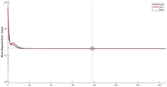
Figure 2.
Error analysis neural network.
The results from the neural network indicate that the major contribution of the LM methodology is offered by JIT/continuous production flow. In this sense, a productivity bonus shares for the workers based on the top 10 metrics classified using the Hesitant Fuzzy Linguistic Term and the TOPSIS method. Similarly, we plan to develop a waste minimization project to take into account the ranking results obtained from the assessments. Additionally, a sensitivity analysis was planted, which implies the comparisons with other methods in order to check the stability of our application and the results are shown in Figure 3.
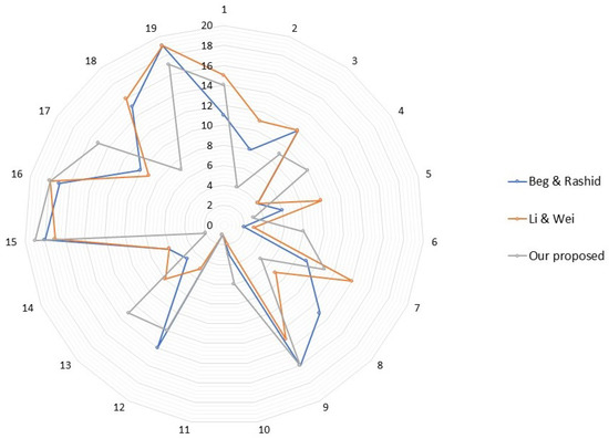
Figure 3.
Sensitivity analysis using other methods.
Observing in Figure 3, we can notice the stability of the gained results. In addition, two different methods were applied and the ranking of the best position does not change. Finally, we demonstrated that there is a significant correspondence between our approach and the two approaches compared.
6. Conclusions
In this research, we propose an operative method for dealing with hesitant assessments in lean manufacturing problems. TOPSIS and HFLTS are a useful tool for managers who wish to assess the KPI’s performance of the LM projects. In this research, we propose a multi-criteria decision-making method to find the desirable alternatives. Likewise, the results from our proposed can be used to design an action plan. Normally, developing cost minimization projects in a manufacturing environment is challenging, yet HFLTS and TOPSIS offer a systematic method for establishing priorities, thereby helping managers determine what key performance indicators (KPIs) have a low performance. Finally, the results represent a robust solution to deal with KPI assessments and provides visibility in terms of how lean manufacturing projects impact corporate performance. In addition, we present the use of AHP in order to determine the weights of criteria. There are some guidelines for future research where MCDM problems exist within the context of HSFLT situations—for example, evaluating the Lean Six Sigma projects, appraising performance of supply chains, among others. In addition, the consideration of the comparisons with other methods of MCDM.
Author Contributions
Conceptualization, L.P.-D. and D.L.-C.; methodology, L.P.-D.; validation, L.P.-D. and J.I.H.H.; formal analysis, D.L.-C.; investigation, L.P.-D. and J.I.H.; resources, D.V.R; writing—original draft preparation, L.P.-D. and D.L.-C.; writing—review and editing, M.I.R.B. and J.I.H.H.; visualization, M.I.R.B.; supervision, D.V.R.; project administration, L.P.-D.and D.L.-C. All authors deliver and approved the last version of the manuscript.
Acknowledgments
This research was partially supported with high-tech resources by the project Laboratorio Nacional de Tecnologías de Información and Consejo Nacional de Ciencia y Tecnología.
Conflicts of Interest
The authors declare no conflict of interest.
References
- Shah, R.; Ward, P.T. Lean manufacturing: Context, practice bundles, and performance. J. Oper. Manag. 2003, 21, 129–149. [Google Scholar] [CrossRef]
- Bhamu, J.; Singh Sangwan, K. Lean Manufacturing: Literature Review and Research Issues. Int. J. Oper. Prod. Manag. 2014, 34, 876–940. [Google Scholar] [CrossRef]
- Agarwal, A.; Shankar, R.; Tiwari, M. Modeling the metrics of lean, agile and leagile supply chain: An ANP-based approach. Eur. J. Oper. Res. 2006, 173, 211–225. [Google Scholar] [CrossRef]
- Jasti, N.V.K.; Kodali, R. Lean Production: Literature Review and Trends. Int. J. Prod. Res. 2015, 53, 867–885. [Google Scholar] [CrossRef]
- Mourtzis, D.; Fotia, S.; Vlachou, E. Lean rules extraction methodology for lean PSS design via key performance indicators monitoring. J. Manuf. Syst. 2017, 42, 233–243. [Google Scholar] [CrossRef]
- Sangwa, N.R.; Sangwan, K.S. Development of an integrated performance measurement framework for lean organizations. J. Manuf. Technol. Manag. 2018, 29, 41–84. [Google Scholar] [CrossRef]
- Kang, N.; Zhao, C.; Li, J.; Horst, J.A. A Hierarchical structure of key performance indicators for operation management and continuous improvement in production systems. Int. J. Prod. Res. 2016, 54, 6333–6350. [Google Scholar] [CrossRef] [PubMed]
- Fullerton, R.R.; Kennedy, F.A.; Widener, S.K. Lean manufacturing and firm performance: The incremental contribution of lean management accounting practices. J. Oper. Manag. 2014, 32, 414–428. [Google Scholar] [CrossRef]
- Mrugalska, B.; Wyrwicka, M.K. Towards Lean Production in Industry 4.0. Procedia Eng. 2017, 182, 466–473. [Google Scholar] [CrossRef]
- Melnyk, S.A.; Bititci, U.; Platts, K.; Tobias, J.; Andersen, B. Is Performance Measurement and Management Fit for the Future? Manag. Account. Res. 2014, 25, 173–186. [Google Scholar] [CrossRef]
- Asgari, N.; Darestani, S.A. Application of multi-criteria decision making methods for balanced scorecard: A literature review investigation. Int. J. Serv. Oper. Manag. 2017, 27, 262–283. [Google Scholar]
- Vinodh, S.; Vimal, K.E.K. Thirty criteria based leanness assessment using fuzzy logic approach. Int. J. Adv. Manuf. Technol. 2012, 60, 1185–1195. [Google Scholar] [CrossRef]
- Susilawati, A.; Tan, J.; Bell, D.; Sarwar, M. Fuzzy logic based method to measure degree of lean activity in manufacturing industry. J. Manuf. Syst. 2015, 34, 1–11. [Google Scholar] [CrossRef]
- Mardani, A.; Zavadskas, E.K.; Khalifah, Z.; Jusoh, A.; Nor, K.M. Multiple Criteria Decision-Making Techniques in Transportation Systems: A Systematic Review of the State of the Art Literature. Transport 2016, 31, 359–385. [Google Scholar] [CrossRef]
- Chakraborty, S. Applications of the MOORA method for decision making in manufacturing environment. Int. J. Adv. Manuf. Technol. 2011, 54, 1155–1166. [Google Scholar] [CrossRef]
- Jaganathan, S.; Erinjeri, J.J.; Ker, J. Fuzzy analytic hierarchy process based group decision support system to select and evaluate new manufacturing technologies. Int. J. Adv. Manuf. Technol. 2007, 32, 1253–1262. [Google Scholar] [CrossRef]
- Wang, H.; Xu, Z.; Zeng, X.J. Hesitant fuzzy linguistic term sets for linguistic decision making: Current developments, issues and challenges. Inf. Fusion 2018, 43, 1–12. [Google Scholar] [CrossRef]
- Rodrǵuez, R.M.; Martínez, L.; Herrera, F. Hesitant Fuzzy Linguistic Term Sets for Decision Making. IEEE Trans. Fuzzy Syst. 2012, 20, 109–119. [Google Scholar] [CrossRef]
- Xia, M.; Xu, Z.; Chen, N. Some Hesitant Fuzzy Aggregation Operators with Their Application in Group Decision Making. Group Decis. Negot. 2013, 22, 259–279. [Google Scholar] [CrossRef]
- Liao, H.; Xu, Z.; Herrera-Viedma, E.; Herrera, F. Hesitant Fuzzy Linguistic Term Set and Its Application in Decision Making: A State-of-the-Art Survey. Int. J. Fuzzy Syst. 2018, 20, 2084–2110. [Google Scholar] [CrossRef]
- Hwang, C.L.; Yoon, K. Multiple Attribute Defecation Making Methods and Applications: A State-of-the-Art Survey; Springer: Berlin, Germany, 1981. [Google Scholar]
- Yue, Z. Knowledge-Based Systems An extended TOPSIS for determining weights of decision makers with interval numbers. Knowl.-Based Syst. 2011, 24, 146–153. [Google Scholar] [CrossRef]
- Behzadian, M.; Khanmohammadi Otaghsara, S.; Yazdani, M.; Ignatius, J. A state-of the-art survey of TOPSIS applications. Expert Syst. Appl. 2012, 39, 13051–13069. [Google Scholar] [CrossRef]
- Sirisawat, P.; Kiatcharoenpol, T. Fuzzy AHP-TOPSIS approaches to prioritizing solutions for reverse logistics barriers. Comput. Ind. Eng. 2018, 117, 303–318. [Google Scholar] [CrossRef]
- Chen, C.T. Extensions of the TOPSIS for group decision-making under fuzzy environment. Fuzzy Sets Syst. 2000, 114, 1–9. [Google Scholar] [CrossRef]
- Beg, I.; Rashid, T. TOPSIS for Hesitant Fuzzy Linguistic Term Sets. Int. J. Intell. Syst. 2013, 28, 1162–1171. [Google Scholar]
- Ren, F.; Kong, M.; Pei, Z. A new hesitant fuzzy linguistic TOPSIS method for group multi-criteria linguistic decision making. Symmetry 2017, 9, 289. [Google Scholar] [CrossRef]
- Li, P.; Wei, C. A Case-Based Reasoning Decision-Making Model for Hesitant Fuzzy Linguistic Information. Int. J. Fuzzy Syst. 2018, 20, 2175–2186. [Google Scholar] [CrossRef]
- Xu, Z. Uncertain linguistic aggregation operators based approach to multiple attribute group decision making under uncertain linguistic environment. Inf. Sci. 2004, 168, 171–184. [Google Scholar] [CrossRef]
- Zhou, W.; Xu, Z. Generalized asymmetric linguistic term set and its application to qualitative decision making involving risk appetites. Eur. J. Oper. Res. 2016, 254, 610–621. [Google Scholar] [CrossRef]
- Farhadinia, B. Multiple criteria decision-making methods with completely unknown weights in hesitant fuzzy linguistic term setting. Knowl.-Based Syst. 2016, 93, 135–144. [Google Scholar] [CrossRef]
- Ming, T.; Liao, H. Managing Information Measures for Hesitant Fuzzy Linguistic Term Sets and Their Applications in Designing Clustering Algorithms. Information 2019. [Google Scholar] [CrossRef]
- Saaty, R.W. The Analytic Hierarchy Process-What and How It is used. Math. Model. 1987, 9, 161–176. [Google Scholar] [CrossRef]
© 2019 by the authors. Licensee MDPI, Basel, Switzerland. This article is an open access article distributed under the terms and conditions of the Creative Commons Attribution (CC BY) license (http://creativecommons.org/licenses/by/4.0/).