Coordinated Dispatch of Multi-Energy Microgrids and Distribution Network with a Flexible Structure


Abstract
1. Introduction
- (1)
- Many literatures only consider the optimal operation of the MG itself, but do not consider the working status of the DN connected to the MG, which will have a bad impact on the entire distribution system;
- (2)
- Some other literature only considers the dispatch of electric loads when considering the optimal joint dispatching of the MG and the DN regardless of other types of loads;
- (3)
- A few works in the literature consider the joint dispatch of multi-energy MGs and the DN but do not consider the topology and power flow of the distribution network itself.
- (1)
- Cooling and heating loads are taken into consideration, which will increase the complementary use of energy and more dispatch flexibility.
- (2)
- The load flow optimization problem of the DN under the integration of the multi-MGs is considered, the aim of which is to improve the operation conditions (minimize the power loss and voltage offset of the DN) and to make the model more accurate.
- (3)
- The DN reconfiguration is included in the proposed method to make further efforts to optimize the operation mode and the security of the DN under the integration of MGs and to improve control flexibility with limited control actions, which will also make the MGs sacrifice the minimum economic benefit under the framework of the coordinated dispatch method.
2. Mathematical Model Formulation
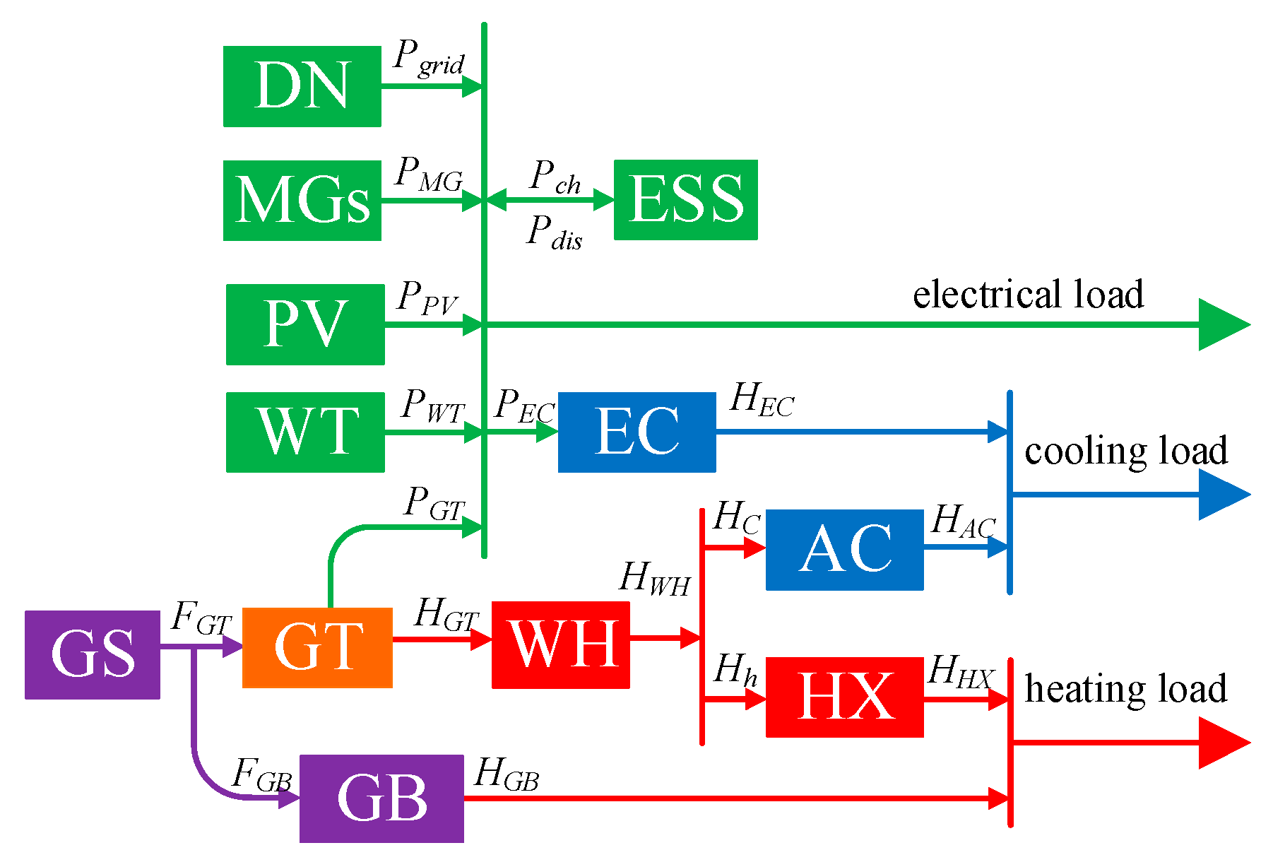
2.1. Multi-Energy Microgrids
2.1.1. Gas Turbine (GT)
2.1.2. Gas Boiler (GB)
2.1.3. Waste-Heat Boiler (WH)
2.1.4. Heat-Exchange Devices (HX)
2.1.5. Absorption Chiller (AC)
2.1.6. Electric Chiller (EC)
2.1.7. Energy Storage System (ESS)
2.1.8. Tie Lines
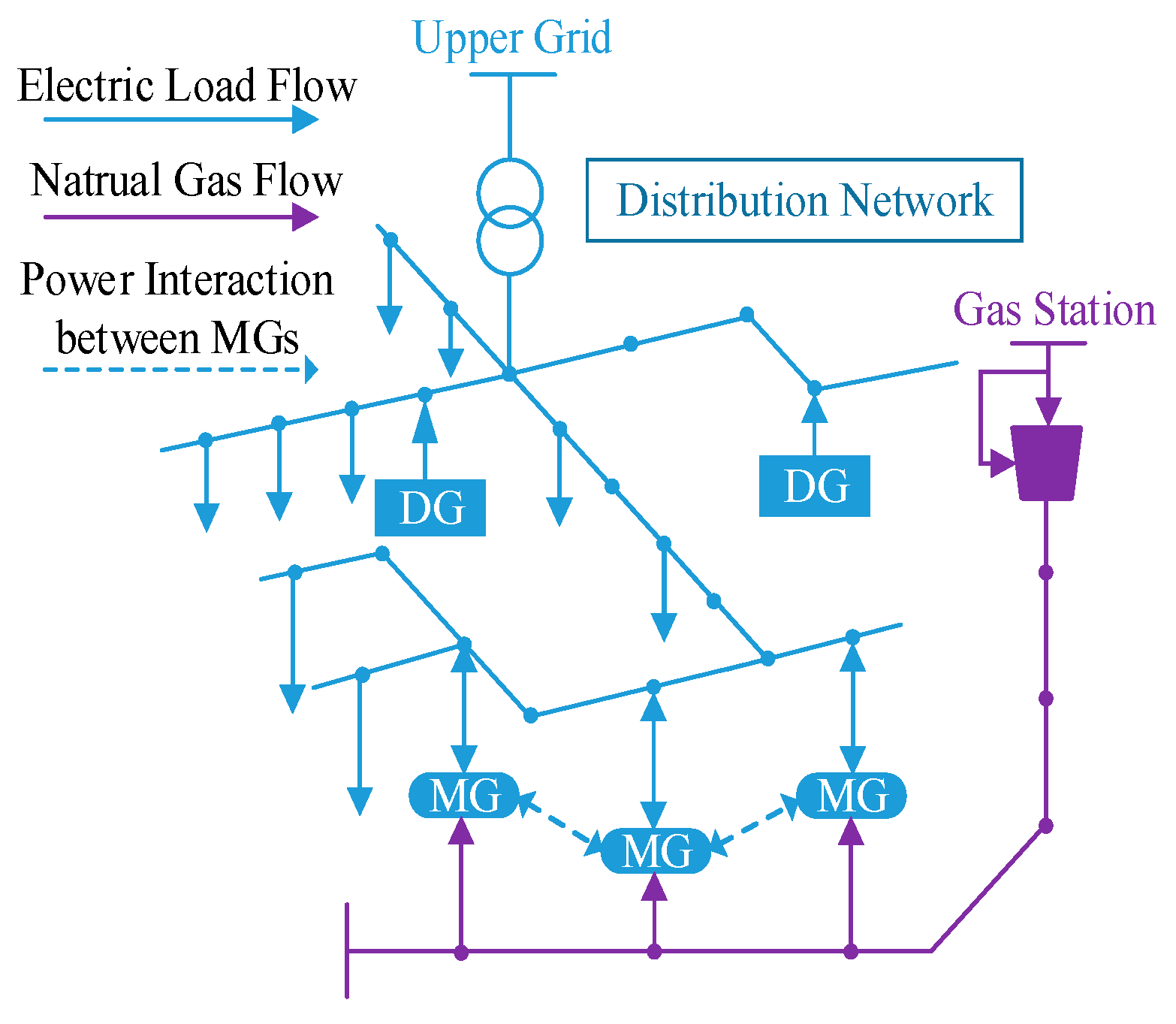
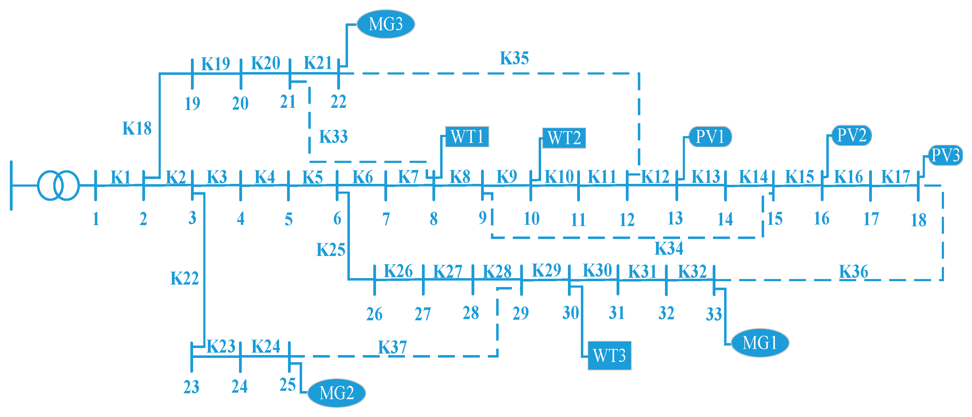
2.2. Distribution Network (DN)
3. Objective Function Formulation
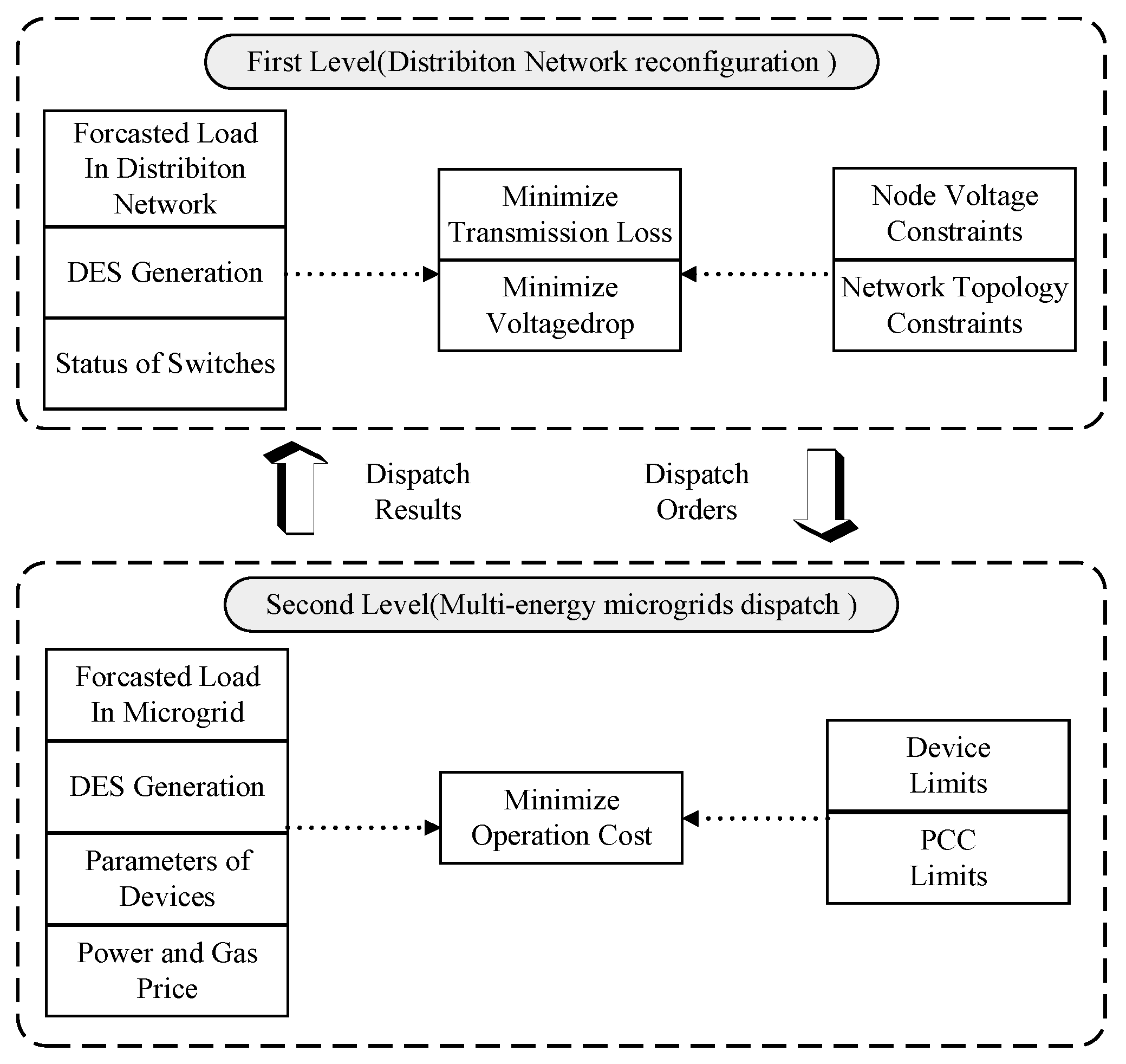
3.1. First Level
3.2. Second Level
- Electric bus balance
- Cooling load bus balance
- Heating load bus balance
- Steam bus balance:where PLoad(t), Hcooling(t), Hheating(t) represent the electrical load, cooling load and heating load, respectively.
4. Solving Method
4.1. First Level
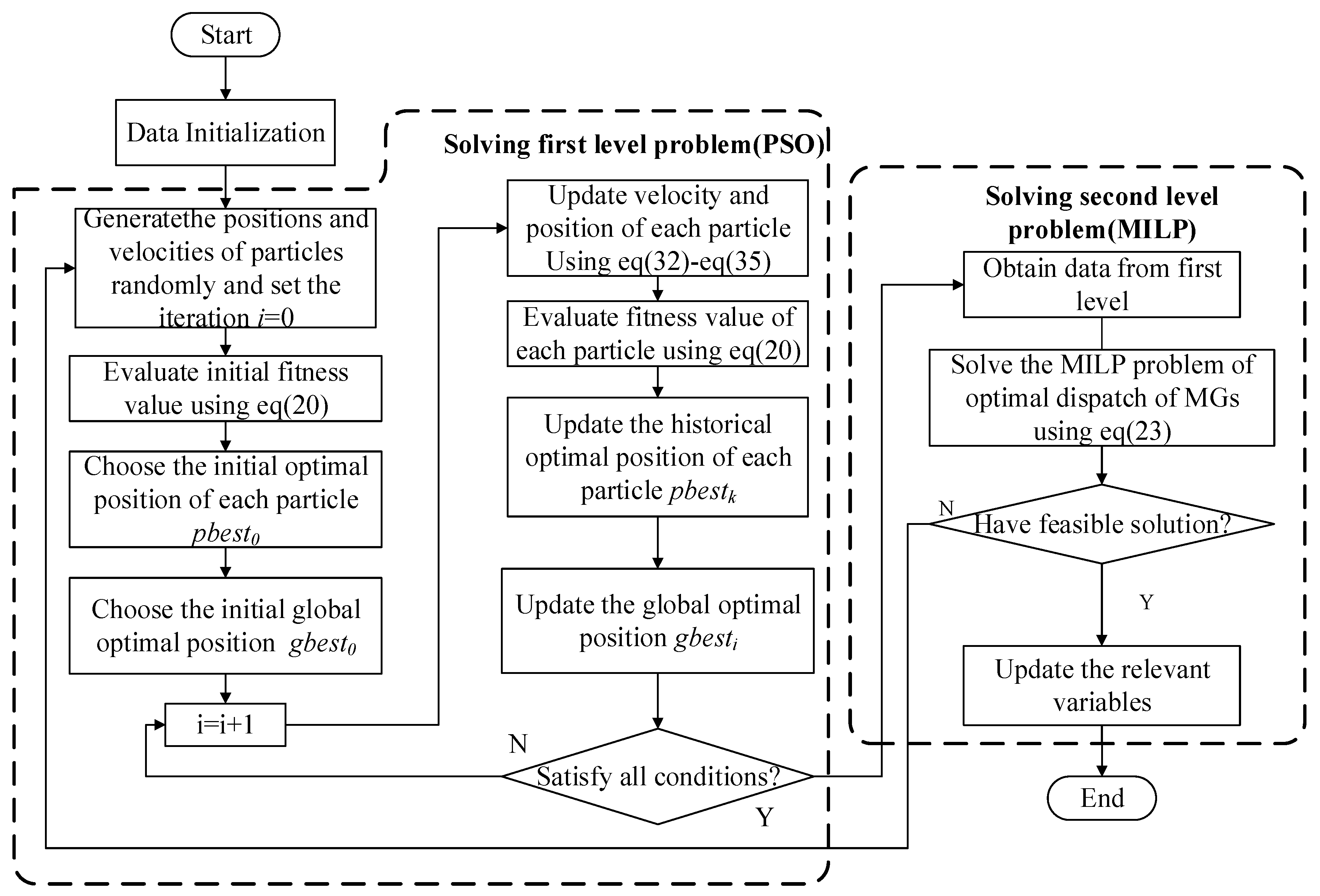
- Step 1: Initialization, acquire the system data, including line and bus parameters, generation information and states of switches. Generate a particle swarm with a sample number of M. Initialize the position x0,k (including the vectors SW and Φ in Equation (21)) and speed v0,k of each particle. Set pbestk = x0,k, evaluate the fitness value fit(x0,k) of each particle using the function in Equation (20) by power flow calculation. Find the particles with the minimum fitness value of all particles and set its position to gbest0.
- Step 2: For ith iteration. Update the position and speed of each particle using Equations (32) and (33), evaluate the fitness value fit(xi,k) of each particle using the function in Equation (20).where rand1(), rand2() represents random numbers between 0 and 1. c1, c2 are learning factors, w is the inertia weight. If the particles are discrete variables like the state of the ith switch si,t in the vector SW, the following rules are required when performing speed updates:where S(Vk) is a Sigmoid function, which is used to select the probability of discrete variable positions. Generate a random number randi,k() between 0 and 1 and compare it with S(vi,k) to determine the value of the binary variable xi,k.
- Step 3: For each particle, compare the fitness value fit(xi,k) with fit(pbestk), update pbestk to the position with lower fitness value.
- Step 4: For all particles, select the particle who has the lowest fitness value. Update gbesti to its position.
- Step 5: Judge whether the result meets the end condition. If the iteration number has reached the upper limit or the fitness value convergence, the calculation stops. Otherwise, return to Step 2.
4.2. Second Level
- Step 1: Aquire the power interaction command vector Φ from the first level, and calculate the solution of the MGs according to the power command.
- Step 2: Judge whether there is a solution for the optimization of the second level. If the solution exists, feedback the information to the first level. If the solution does not exist, it needs to change the operation method (regardless of upper DN) and re-solve the first level. The flow chart of the solution process above is shown in Figure 4.
5. Simulation Result
5.1. Case Set Up
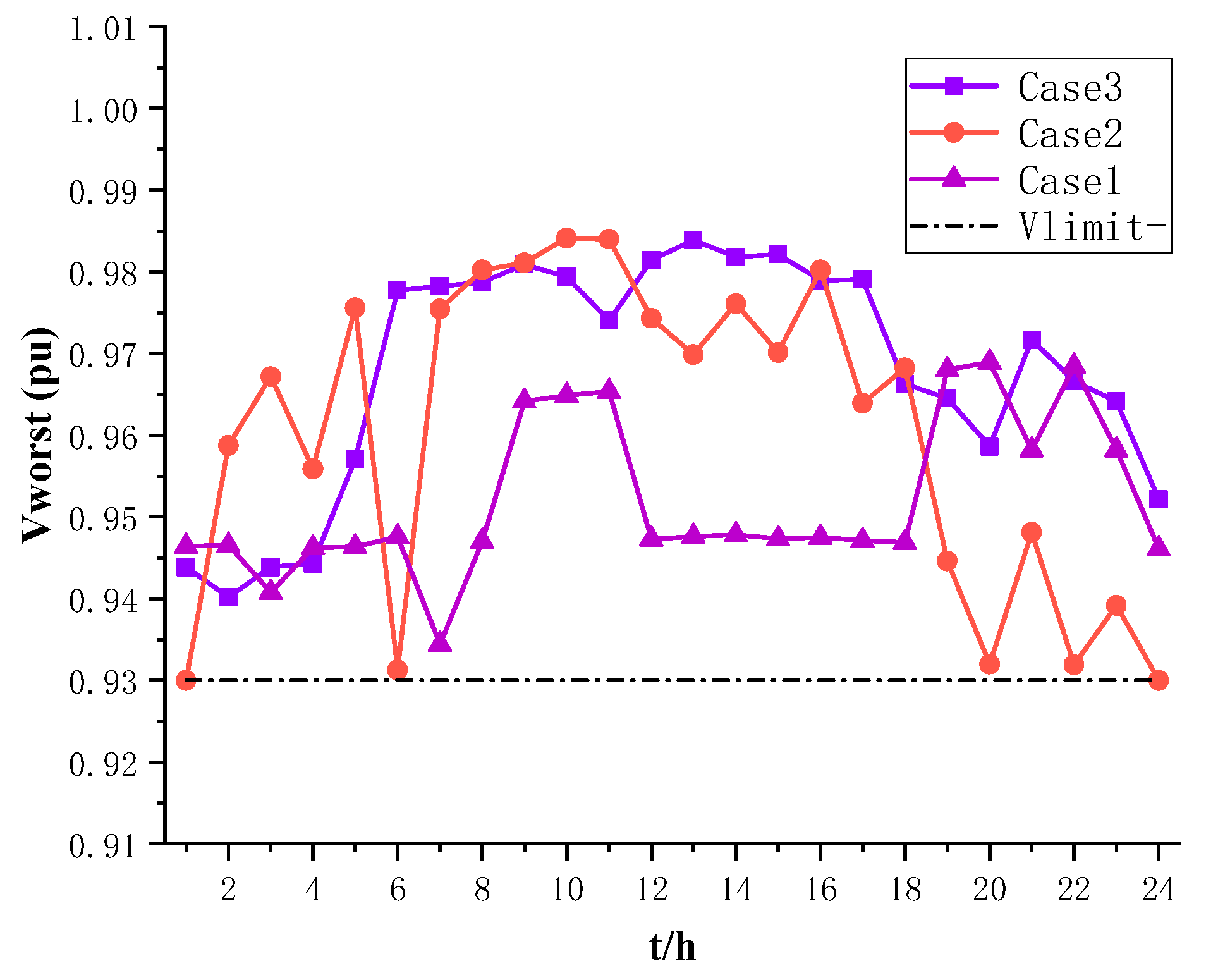
- Case 1: Optimal dispatch of MGs. MGs purchase or sell power to DN and buy natural gas from the gas network without consideration of the DN [15].
- Case 2: Optimal dispatch of MGs and operation of DN (considering power loss) without consideration of the DN reconfiguration [29].
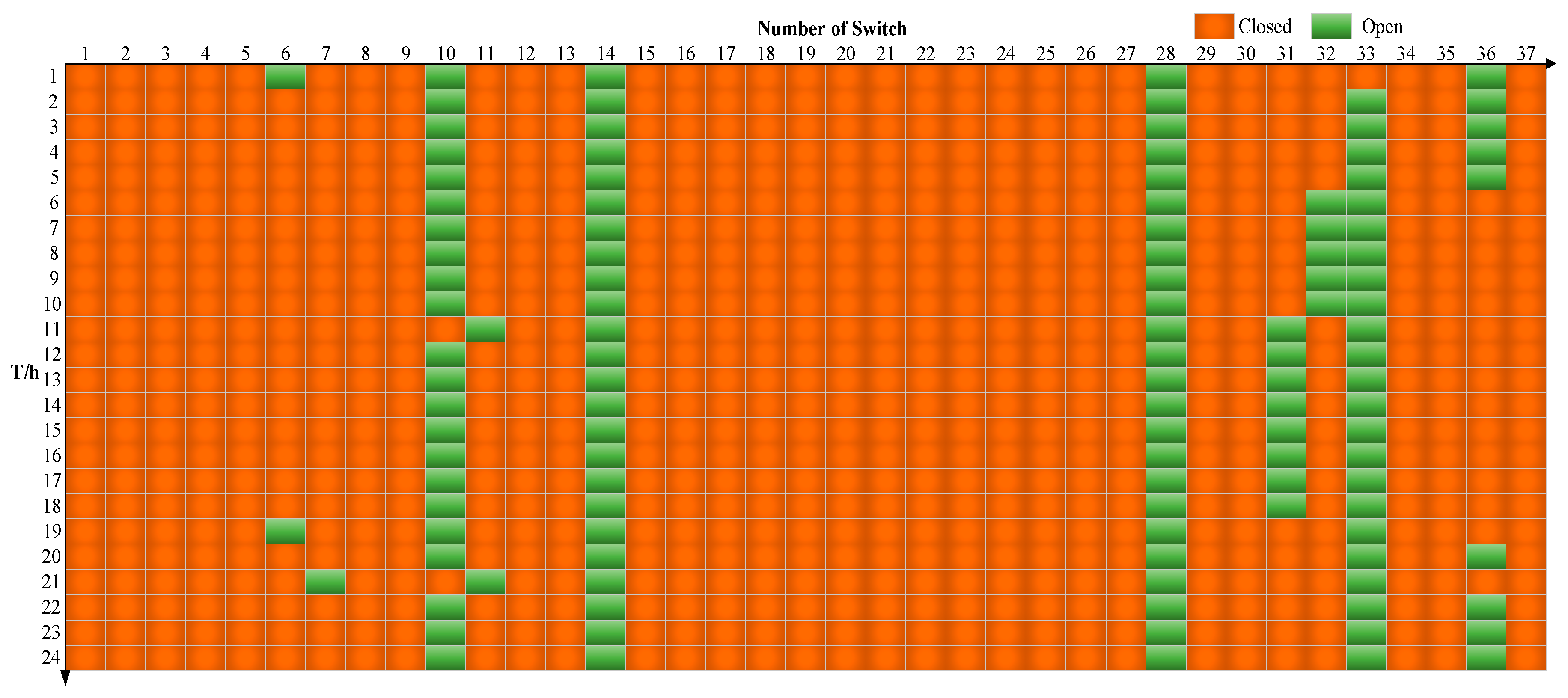
- Case 3: The method proposed in this paper. The bi-level optimal dispatch considering operations of MGs and DN considering reconfiguration, through controlling the switch on each tie line in DN, operating condition of devices and power interaction of the PCC (point of common coupling, the connection point between the MG and the DN).
5.2. Result Analysis
5.2.1. First Level
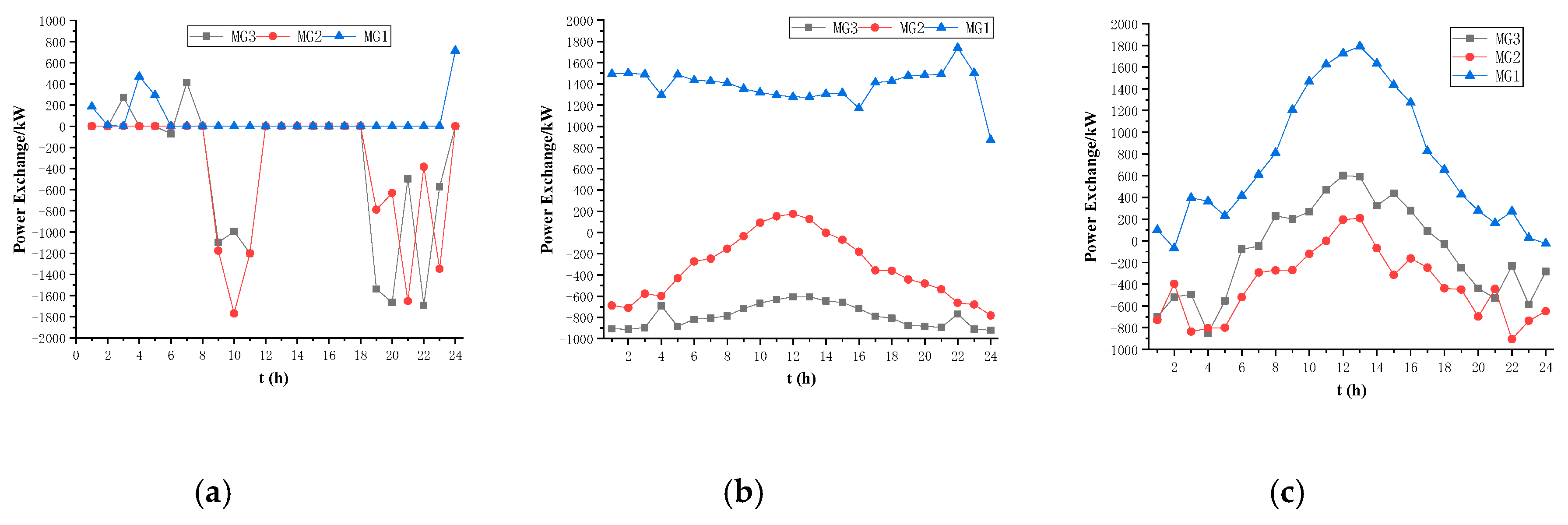
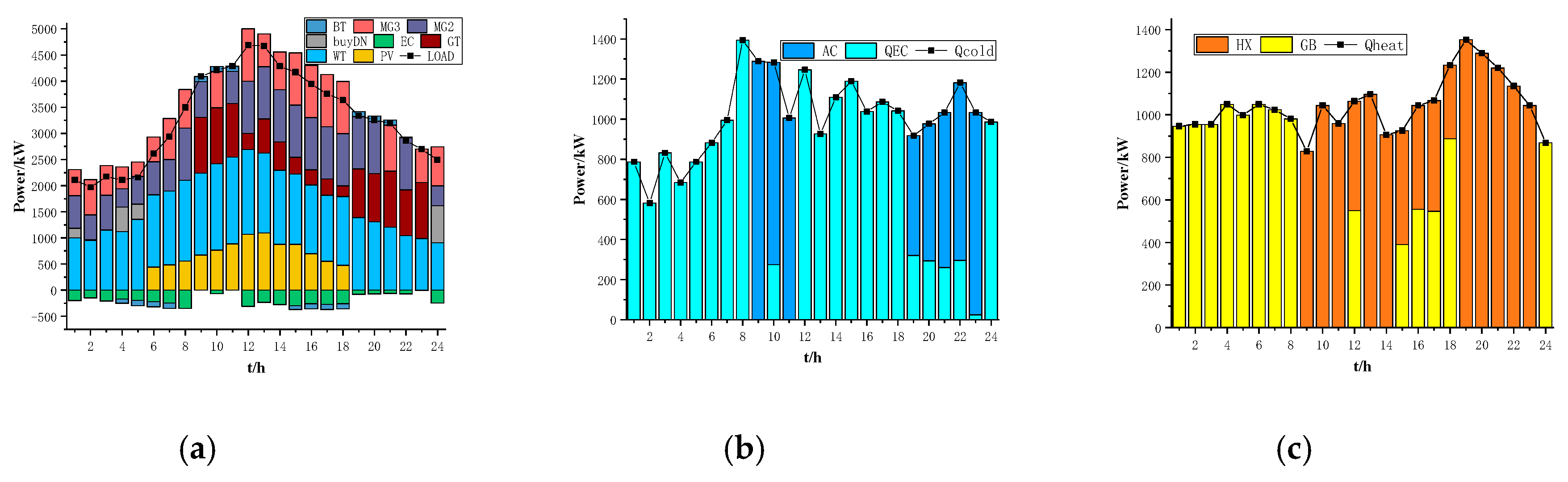
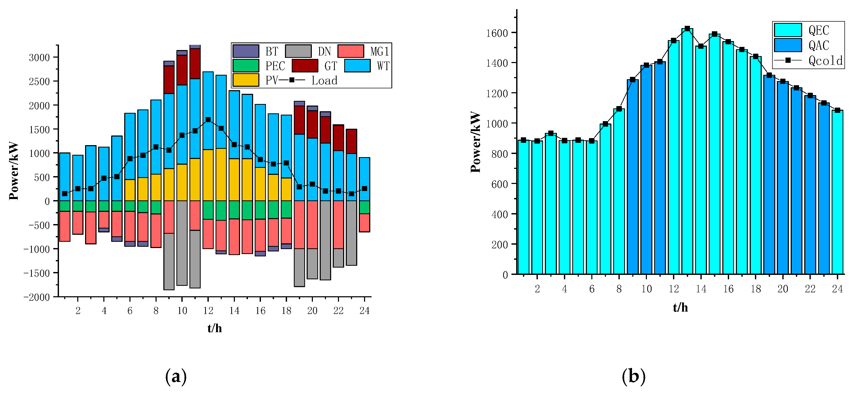
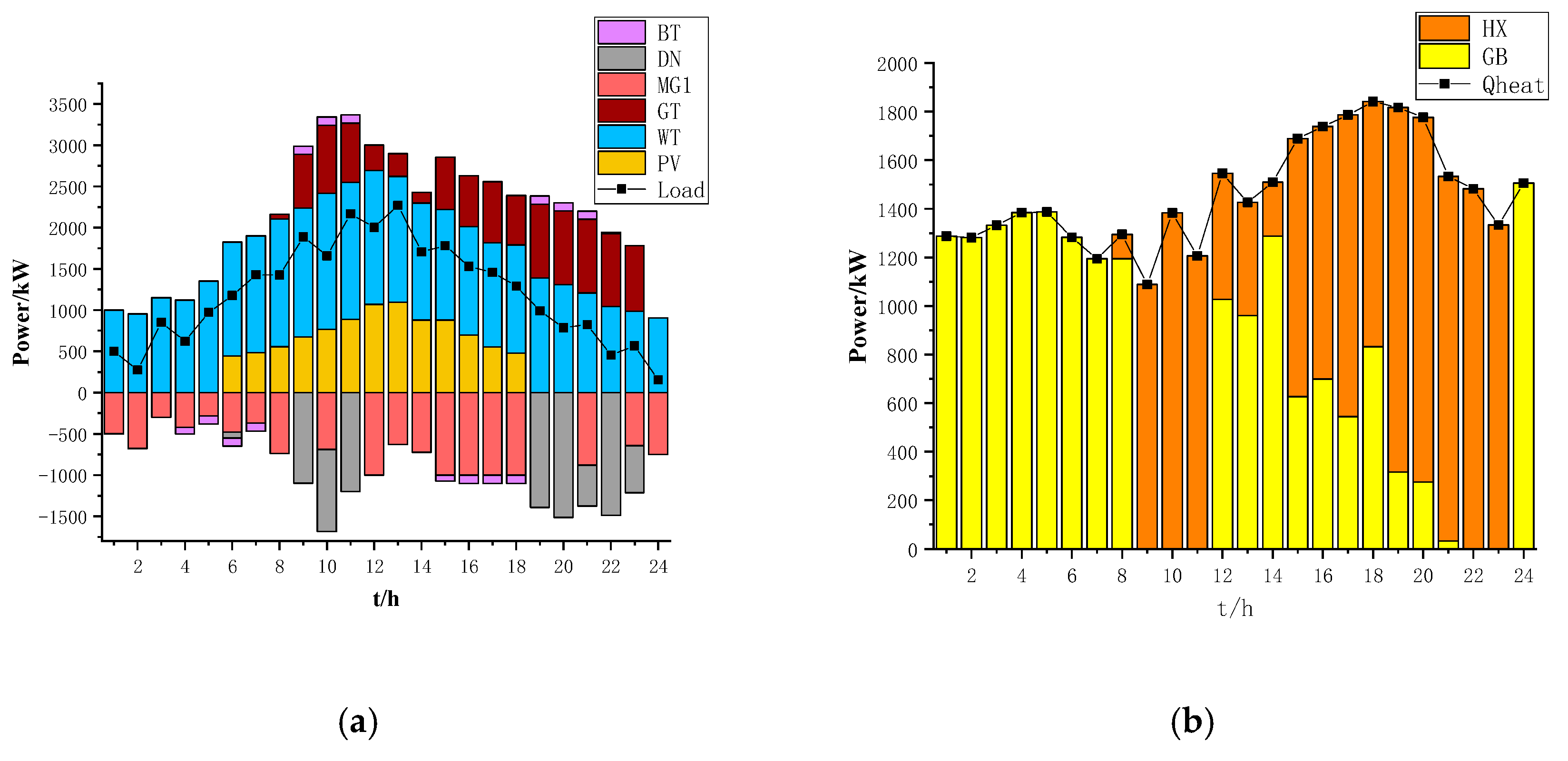
5.2.2. Second Level
5.2.3. Summary
6. Conclusions
- (1)
- The power loss, voltage offset, and power interaction on tie lines have noticeable reductions based on the proposed method, reflecting that it is necessary to consider both the benefit of DN and MGs.
- (2)
- Compared with [25], the consideration of the structure of the DN can keep the voltage of partial nodes away from extreme conditions, while further reducing DN power loss and operating costs of the MGs.
- (3)
- The MGs provide support for the DN, and in the appropriate cases, some of the benefits can be sacrificed to meet the dispatch requirements under the framework proposed in this paper.
- (4)
- This paper only considers the electrical distribution network. Further research can focus on the effect of taking gas networks and thermal networks into consideration.
Author Contributions
Funding
Conflicts of Interest
References
- Li, J.; Ying, Y.; Lou, X.; Fan, J.; Chen, Y.; Bi, D. Integrated Energy System Optimization Based on Standardized Matrix Modeling Method. Appl. Sci. 2018, 8, 2372. [Google Scholar] [CrossRef]
- Lopes, J.A.P.; Hatziargyriou, N.; Mutale, J.; Djapic, P.; Jenkins, N. Integrating distributed generation into electric power systems: A review of drivers, challenges and opportunities. Electr. Power Syst. Res. 2007, 77, 1189–1203. [Google Scholar] [CrossRef]
- García Vera, Y.E.; Dufo-López, R.; Bernal-Agustín, J.L. Energy Management in Microgrids with Renewable Energy Sources: A Literature Review. Appl. Sci. 2019, 9, 3854. [Google Scholar] [CrossRef]
- Lahon, R.; Gupta, C.P. Energy management of cooperative microgrids with high-penetration renewables. IET Renew. Power Gener. 2018, 12, 680–690. [Google Scholar] [CrossRef]
- Geidl, M.; Koeppel, G.; Favre-Perrod, P.; Klockl, B.; Andersson, G.; Frohlich, K. Energy hubs for the future. IEEE Power Energy Mag. 2007, 5, 24–30. [Google Scholar] [CrossRef]
- Huang, A.Q.; Crow, M.L.; Heydt, G.T.; Zheng, J.P.; Dale, S.J. The Future Renewable Electric Energy Delivery and Management (FREEDM) System: The Energy Internet. Proc. IEEE 2011, 99, 133–148. [Google Scholar] [CrossRef]
- Li, H.; Fu, L.; Geng, K.; Jiang, Y. Energy utilization evaluation of CCHP systems. Energy Build. 2006, 38, 253–257. [Google Scholar] [CrossRef]
- Liu, M.; Shi, Y.; Fang, F. A new operation strategy for CCHP systems with hybrid chillers. Appl. Energy 2012, 95, 164–173. [Google Scholar] [CrossRef]
- Sanaye, S.; Hajabdollahi, H. 4E analysis and multi-objective optimization of CCHP using MOPSOA. Proc. Inst. Mech. Eng. Part E J. Process. Mech. Eng. 2012, 228, 43–60. [Google Scholar] [CrossRef]
- Carvalho, M.; Serra, L.M.; Lozano, M.A. Optimal synthesis of trigeneration systems subject to environmental constraints. Energy 2011, 36, 3779–3790. [Google Scholar] [CrossRef]
- Ahn, S.; Moon, S. Economic scheduling of distributed generators in a microgrid considering various constraints. In Proceedings of the 2009 IEEE Power & Energy Society General Meeting, Calgary, AB, Canada, 26–30 July 2009; pp. 1–6. [Google Scholar]
- Wang, C.S.; Hong, B.W.; Guo, L. A general modeling method for optimal dispatch of combined cooling, heating and power microgrid. Proc. CSEE 2013, 33, 26–33. [Google Scholar]
- Liu, C.; Wang, X.; Wu, X.; Guo, J. Economic scheduling model of microgrid considering the lifetime of batteries. IET Gener. Transm. Distrib. 2017, 11, 759–767. [Google Scholar] [CrossRef]
- Kang, L.; Yang, J.; An, Q.; Deng, S.; Zhao, J.; Wang, H.; Li, Z. Effects of load following operational strategy on CCHP system with an auxiliary ground source heat pump considering carbon tax and electricity feed in tariff. Appl. Energy 2017, 194, 454–466. [Google Scholar] [CrossRef]
- Xu, Q.S.; Li, L.; Cai, J.L.; Luan, K.N.; Yang, B. Day-ahead Optimized Economic Dispatch of CCHP Multi-microgrid System Considering Power Interaction among Microgrids. Autom. Electr. Power Syst. 2018, 42, 36–46. [Google Scholar]
- Liu, N.; Wang, J.; Wang, L. Hybrid Energy Sharing for Multiple Microgrids in an Integrated Heat–Electricity Energy System. IEEE Trans. Sustain. Energy 2019, 10, 1139–1151. [Google Scholar] [CrossRef]
- Bui, V.; Hussain, A.; Im, Y.; Kim, H. An internal trading strategy for optimal energy management of combined cooling, heat and power in building microgrids. Appl. Energy 2019, 239, 536–548. [Google Scholar] [CrossRef]
- Li, Y.; Zou, Y.; Tan, Y.; Cao, Y.; Liu, X.; Shahidehpour, M.; Tian, S.; Bu, F. Optimal Stochastic Operation of Integrated Low-Carbon Electric Power, Natural Gas, and Heat Delivery System. IEEE Trans. Sustain. Energy 2018, 9, 273–283. [Google Scholar] [CrossRef]
- Bazmohammadi, N.; Tahsiri, A.; Anvari-Moghaddam, A.; Guerrero, J.M. A hierarchical energy management strategy for interconnected microgrids considering uncertainty. Int. J. Electr. Power Energy Syst. 2019, 109, 597–608. [Google Scholar] [CrossRef]
- Wang, J.; Zhong, H.; Xia, Q.; Kang, C.; Du, E. Optimal joint-dispatch of energy and reserve for CCHP-based microgrids. IET Gener. Transm. Distrib. 2017, 11, 785–794. [Google Scholar] [CrossRef]
- Rakipour, D.; Barati, H. Probabilistic optimization in operation of energy hub with participation of renewable energy resources and demand response. Energy 2019, 173, 384–399. [Google Scholar] [CrossRef]
- Gu, W.; Lu, S.; Wu, Z.; Zhang, X.; Zhou, J.; Zhao, B.; Wang, J. Residential CCHP microgrid with load aggregator: Operation mode, pricing strategy, and optimal dispatch. Appl. Energy 2017, 205, 173–186. [Google Scholar] [CrossRef]
- Di Manno, M.; Varilone, P.; Verde, P.; De Santis, M.; Di Perna, C.; Salemme, M. in User friendly smart distributed measurement system for monitoring and assessing the electrical power quality. In Proceedings of the 2015 AEIT International Annual Conference (AEIT), Naples, Italy, 14–16 October 2015; pp. 1–5. [Google Scholar]
- Di Fazio, A.; Russo, M.; De Santis, M. Zoning Evaluation for Voltage Optimization in Distribution Networks with Distributed Energy Resources. Energies 2019, 12, 390. [Google Scholar] [CrossRef]
- Yuen, C.; Oudalov, A. The Feasibility and Profitability of Ancillary Services Provision from Multi-MicroGrids. In Proceedings of the 2007 IEEE Lausanne Power Tech, Lausanne, Switzerland, 1–5 July 2007; pp. 598–603. [Google Scholar]
- Nikmehr, N.; Najafi Ravadanegh, S. Optimal Power Dispatch of Multi-Microgrids at Future Smart Distribution Grids. IEEE Trans. Smart Grid. 2015, 6, 1648–1657. [Google Scholar] [CrossRef]
- Wu, J.; Guan, X. Coordinated Multi-Microgrids Optimal Control Algorithm for Smart Distribution Management System. IEEE Trans. Smart Grid. 2013, 4, 2174–2181. [Google Scholar] [CrossRef]
- Gao, Y.; Ai, Q. Hierarchical Coordination Control for Interconnected Operation of Electric-thermal-gas Integrated Energy System with Micro-energy Internet Clusters. IEEE J. Emerg. Sel. Top. Power Electron. 2018, 1. [Google Scholar] [CrossRef]
- Xu, Q.; Li, L.; Sheng, Y.; Huo, X.; Zhao, B. Day-Ahead Optimized Economic Dispatch of Active Distribution Power System with Combined Cooling, Heating and Power-Based Microgrids. Power Syst. Technol. 2018, 42, 1726–1735. [Google Scholar]
- Golshannavaz, S.; Afsharnia, S.; Aminifar, F. Smart Distribution Grid: Optimal Day-Ahead Scheduling With Reconfigurable Topology. IEEE Trans Smart Grid 2014, 5, 2402–2411. [Google Scholar] [CrossRef]
- Shan, G.; Liu, J.H. Research on the distribution network reconfiguration with the distributed generation. Power Syst. Prot. Control. 2015, 31, 52–57. [Google Scholar]
- Zhai, H.F.; Yang, M.; Chen, B.; Kang, N. Dynamic reconfiguration of three-phase unbalanced distribution networks. Int. J. Electr. Power Energy Syst. 2018, 99, 1–10. [Google Scholar] [CrossRef]
- Di Fazio, A.R.; Russo, M.; Pisano, G.; De Santis, M. A centralized voltage optimization function exploiting DERs for distribution systems. In Proceedings of the 2019 International Conference on Clean Electrical Power (ICCEP), Otranto, Italy, 2–4 July 2019; pp. 100–109. [Google Scholar]


| Symbol | Definition | Symbol | Definition |
|---|---|---|---|
| PV | Photovoltaic array | ESS | Energy storage system |
| WT | Wind turbine | EC | Electric chiller |
| GS | Gas station | AC | Absorption chiller |
| GB | Gas boiler | GT | Gas turbine |
| WH | Waste heat boiler | HX | Heat exchanger |
| Parameters | Values | Parameters | Values |
|---|---|---|---|
| ηWH | 0.8 | 2000 kW | |
| ηGB | 0.9 | 1500 kW | |
| ηHX | 0.9 | 1000 kW | |
| COPAC | 1.2 | 100 kW | |
| COPEC | 4 | 100 kW | |
| ηch/ηdis | 0.96 | 0.9 | |
| δ | 0.02 | 0.2 | |
| 1500 kW | 2000 kW | ||
| 2000 kW | 1000 kW |
| Time Slot | Price between DN and MGs | Price between MGs |
|---|---|---|
| 23:00–7:00 | 0.17 | 0.12 |
| 7:00–8:00 17:00–18:00 | 0.49 | 0.37 |
| 8:00–11:00 18:00–23:00 | 0.83 | 0.65 |
| MGs Optimal Dispatch | Operation of DN | DN Reconfiguration | |
|---|---|---|---|
| Case1 | √ | × | × |
| Case2 | √ | √ | × |
| Case3 | √ | √ | √ |
| Result | Case 1 | Case 2 | Case 3 |
|---|---|---|---|
| Ploss/MW | 2.5310 | 2.1543 | 1.8015 |
| Voff/pu | 12.6580 | 9.9851 | 9.0416 |
| Case 1 | Case 2 | Case 3 | |
|---|---|---|---|
| MG1 | 28,173.95 | 33,338.42 | 31,646.77 |
| MG2 | −2773.21 | −1986.90 | −3012.89 |
| MG3 | 7558.35 | 9433.32 | 8802.69 |
| Total | 33,059.09 | 40,784.84 | 37,436.03 |
© 2019 by the authors. Licensee MDPI, Basel, Switzerland. This article is an open access article distributed under the terms and conditions of the Creative Commons Attribution (CC BY) license (http://creativecommons.org/licenses/by/4.0/).
Share and Cite
Chen, S.; Yang, Y.; Xu, Q.; Zhao, J. Coordinated Dispatch of Multi-Energy Microgrids and Distribution Network with a Flexible Structure. Appl. Sci. 2019, 9, 5553. https://doi.org/10.3390/app9245553
Chen S, Yang Y, Xu Q, Zhao J. Coordinated Dispatch of Multi-Energy Microgrids and Distribution Network with a Flexible Structure. Applied Sciences. 2019; 9(24):5553. https://doi.org/10.3390/app9245553
Chicago/Turabian StyleChen, Sijie, Yongbiao Yang, Qingshan Xu, and Jun Zhao. 2019. "Coordinated Dispatch of Multi-Energy Microgrids and Distribution Network with a Flexible Structure" Applied Sciences 9, no. 24: 5553. https://doi.org/10.3390/app9245553
APA StyleChen, S., Yang, Y., Xu, Q., & Zhao, J. (2019). Coordinated Dispatch of Multi-Energy Microgrids and Distribution Network with a Flexible Structure. Applied Sciences, 9(24), 5553. https://doi.org/10.3390/app9245553