1. Introduction
We consider the problem of estimation of the signal-to-noise ratio (SNR) when a deterministic real sinusoid with unknown parameters is corrupted by additive white Gaussian noise. This problem is encountered in different fields of engineering; for example, in telecommunications [
1], in radar systems [
2] and in smart-grid applications. Indeed, this study started from the need for accurate measurement of the SNR in a test-bed used for synchrophasor measurement before estimation of the parameters of the sinusoidal voltage [
3,
4].
The same problem has been studied in [
5], wherein Papic et al. proposed an algorithm for SNR estimation based on autocorrelation and modified covariance methods for autoregressive spectral estimation and required the reliable estimate of the frequency of the sinusoid. The case of
complex rather than
real deterministic sinusoids in additive noise has been addressed in [
6], wherein an SNR estimator derived with the method of moments [
7] that makes use of second and fourth order moments was proposed (
-estimator). It does not require the complex sinusoid frequency estimate, and for this reason, it belongs to the class of blind SNR estimators and may find applications in all those cases where the frequency estimate may not be available or frequency may be varying over the observation interval.
In recent years, moment-based SNR estimators have attracted the interest of researchers in the telecommunications field where second and fourth order moments based estimators have been employed for estimation of the SNR of modulated signals in additive white Gaussian noise and flat-fading channels. In [
1,
8], for example, the SNR
-estimator was proposed for phase-shift keying (PSK) modulated signals as a blind estimator that does not require the knowledge of transmitted data. In [
9] more general moments-based SNR estimators were derived for multi-level constellations, such as generic quadrature amplitude modulation (QAM) constellations, and the SNR
-estimator was derived as a special case of moment-based estimators that make use of higher-order moments. In [
10] an estimator that uses also the sixth-order moment of the received data for non-constant modulus constellations was proposed in order to improve performances. Further extensions of the method for multilevel constellations were proposed in [
11]. In [
9,
10,
11] performances of the proposed estimators were theoretically studied and results based on asymptotic analyses were reported.
In this paper we propose a moment-based SNR estimator for a deterministic real sinusoid in additive noise that is formed by the ratio of the estimators of the signal power and noise power. The proposed estimators belong to the class of the second-and-fourth-order moments estimators that can be obtained by application of the method of moments [
7] and do not require the reliable frequency estimate, as in [
5]. We derived a new general formula for even-order moments of the observed signal that is useful not only to provide the second and fourth moments required by the method of moments, but also for the study of statistical performances of the proposed estimators. Since asymptotic analyses carried out in [
9,
10,
11] assume random signals in random noise and cannot immediately be extended to deterministic signals, we also derived a new general expression for covariance matrices useful for asymptotic analysis of performances of moment-based estimators when the signal corrupted by the noise is deterministic. Results from asymptotic analyses and Monte-Carlo simulations are presented along with the corresponding Cramer–Rao lower bounds (CRLB), and we reveal that the proposed estimators have good performances in a wide range of operating conditions. In same cases performances are very close to the optimum. This paper extends some of the results presented in [
12] by providing new general formulas for any even-order moments and covariance matrices of the vectors of sample moments, and by studying statistical performances of the proposed estimators with theoretical asymptotic analyses that confirm the numerical results obtained with Monte-Carlo simulations.
The paper is organized as follows: in
Section 2 we derive the estimators starting from a general result on the even-order moment for the given signal model; in
Section 3 we derive the Cramer–Rao lower bounds for all proposed estimators; in
Section 4 the asymptotic performances of the proposed estimators are derived; in
Section 5 results from Monte-Carlo simulations are presented along with comparisons with the CRLBs and the asymptotic performances; finally, in
Section 6 we draw the conclusions.
2. Moment-Based Estimators
We assume that samples from a real sinusoidal signal in additive noise are available over an observation window of size
K, i.e.,
where
; the amplitude
A, the frequency
and phase
of the sinusoid are unknown; and the additive Gaussian noise
is a random variable with zero-mean and unknown variance
; i.e.,
. The signal-to-noise ratio (SNR), defined as
, is then unknown and represents the parameter we wish to estimate when the other parameters of the sinusoid, frequency and phase, remain unknown. To that purpose we derive an estimator based on the method of moments.
The method of moments is a well known statistical method used to derive estimators as functions of sample high-order moments [
7]. The key idea is to express the parameter to be estimated as a function of the moments of
of a different order—i.e.,
, where
m is an integer—and use the natural estimators of the moments
in place of the true moments
to get an estimate of the parameter from the observed samples. In many cases, such estimators are computationally not intensive and present good statistical performances. Though, in general, the optimality of an estimator derived with this method cannot be guaranteed, in many cases the estimator turns out to be consistent. The method relies on the possibility of expressing moments from the observed random signal as functions of the parameters to be estimated. However, when in the observed signal model, one term is deterministic, as is our case, so the derivation of the moments might be cumbersome, as shown, for example, in [
6]. For these cases, Kay suggests to assume a random nature for the "deterministic" sinusoid by assuming a random phase, and in this paper we follow such an approach [
7] (p. 299).
To derive moment-based estimators of the signal power
, noise power
and SNR
we use the second and fourth order moment, and therefore, we need to compute
and
. Instead of deriving each moment separately, as done in [
12], we show here that a general formula expressing any even-order moment of the signal (
1) exists that is valid asymptotically as the number of observed samples grows to infinity. Equivalently, in the signal model (
1), where the sinusoidal signal is deterministic, we assume that the sinusoidal signal’s phase is a uniform random variable (r.v.), i.e.,
, independent of the noise
. Consequently, we can treat the sequence
as the realization of a wide sense stationary (WSS) random sequence for which it is possible to calculate statistical moments as, under the given assumption,
for
.
The general formula for even-order moments for the signal model (
1) is given by the following expression.
where
denotes the double factorial operator and its derivation is given in
Appendix A.
From (
3) we can immediately get the second and fourth moments
Let
and
; then, from (
4) and (
5) we obtain the estimators for
S and
N as
where, as required by the method of moments, instead of the true moments we use their corresponding natural estimators
The SNR estimator is immediately built as the ratio of the two estimators derived above; i.e.,
In the following sections performances of the proposed estimators are studied both theoretically and numerically in terms of squared bias and variance. For a generic estimator
the squared bias is defined as [
7,
13]
while the variance is defined as
3. Cramer–Rao Lower Bounds
Before deriving the performances of the proposed estimators, we derive the corresponding Cramer–Rao lower bounds (CRLB), as they represent the theoretical limit on the best achievable accuracy that can be obtained. First, we derive the CRLB for and and then the CRLB for the estimator of SNR .
We start from the joint probability density function
where
and
. To get the bound we need to first derive the Fisher information matrix that is defined as
In
Appendix B we show that in this case, the Fisher matrix is given by
and the Cramer–Rao lower bounds for the estimators
and
, obtained by inversion of the Fisher matrix, are
Based on the above results it is now possible to derive the CRLB for the proposed SNR estimator
. Since the estimator is formed by the ratio of
and
, the bound for
can be derived from the Fisher information matrix obtained previously and the derivatives of the transformation
according the following relationship [
7]
Similarly, we can derive the bound when the SNR is expressed in dB. In this case the estimator is given by the following transformation
The derivatives are
and we have that the lower bound is
4. Asymptotic Performances
It is only possible to study the analytical performances of the proposed estimators asymptotically, i.e., for
K that tends to infinity. In this section we derive the asymptotic variances of all proposed estimators and we will show in the next section that, though the analysis is only valid for
, in some cases we have found that the analytical results may predict performances for sufficiently high
K as well. Unfortunately, it is not possible to predict the number of samples required to get the asymptotic results and we need to run Monte-Carlo simulations to have an idea of how large the number of samples needs to be. The mathematical method that we apply to derive the asymptotic analytical performances is outlined, for example, in [
7], and makes it possible to overcome the mathematical intractability of the method that uses the transformation of random variables to get the pdf of the estimator.
The variance of the estimator derived with the method of moments can be obtained from the first-order Taylor expansion of
about the point
, where
is the vector of the sample moments and
is the function that maps the sample moments to the estimate. Under the first-order approximation the mean of the estimator is equal to
and by simple substitution using (
4) and (
5) it can be shown that the proposed estimators are asymptotically unbiased. The first-order approximation of the variance is given by
where
is the covariance matrix of
; i.e.,
Hence, we need to derive the covariance matrix under the assumption that in the signal model (
1)
is a deterministic signal. In
Appendix C the covariance matrix is derived and it is shown that we cannot make the assumption suggested by Kay on the deterministic signal
, i.e., assume that such signal is random by assuming a random initial phase, and that the covariance matrix used to get asymptotic results in similar studies [
9,
10,
11] cannot be used here.
Given the signal model (
1) and the vector of even-order sample moments
, each element of the covariance matrix
is
where
and
Note that the same covariance matrix can be used to study the asymptotic performances of all proposed estimators as the only difference is in the way the function
is defined in each case. Furthermore, such a covariance matrix is useful to evaluate the performances of any moment based estimator given the signal model (
1).
To derive the asymptotic variance of all proposed estimators we also need the partial derivatives defined in (
24). As we use the second and fourth moment of
we only need to consider the two sample moments
and
. The derivatives of the function
are easily computed. First, consider the estimator
, that is defined by the following function
Hence, the partial derivatives are
and
The above results are useful for the estimator of the noise power
defined by the function
, as follows.
The corresponding derivatives are
Finally, the derivatives of the function
, that define the estimator of the SNR
, are
The general expression of the covariance matrix shows that the proposed estimators are consistent. However, it is difficult to know in advance when the asymptotic behavior describes the actual performances of the estimators well.
5. Numerical Examples
We present in this section some examples of the performances of the proposed moment-based estimators for
S and
N and signal-to-noise ratio
in terms of squared bias and variance. We report estimated squared biases and variances obtained through Monte-Carlo simulations and we will find that such numerical results confirm the asymptotic performances derived in
Section 4. We also compare them to the corresponding CRLBs derived in
Section 3 and we make some comments on the property of efficiency of the proposed estimators, i.e., whether they achieve (asymptotically) the corresponding CRLB, and on the property of consistency, i.e., whether the variance can be made to approach zero as the number of observations
[
7,
13].
For all proposed estimators we have estimated the squared bias (
11) and variance (
12) by averaging over
estimates on a varying number of observations
K. The mean of each estimator is estimated by means of a standard sample mean estimator; e.g., for
where
is a single estimate of
S with
K observations. The squared bias is then obtained from (
11), where the estimated mean is used in place of the true mean; e.g.,
. The variance of estimators is estimated by means of the standard sample variance estimator; e.g., for
Estimation of squared bias and variance of estimators has been performed at different SNRs that, without loss of generality, are obtained by varying the power of the real sinusoid S while maintaining fixed noise power . The frequency and phase of the deterministic sinusoid were chosen randomly at the beginning of each simulation.
5.1. Performances of
First, we verified that
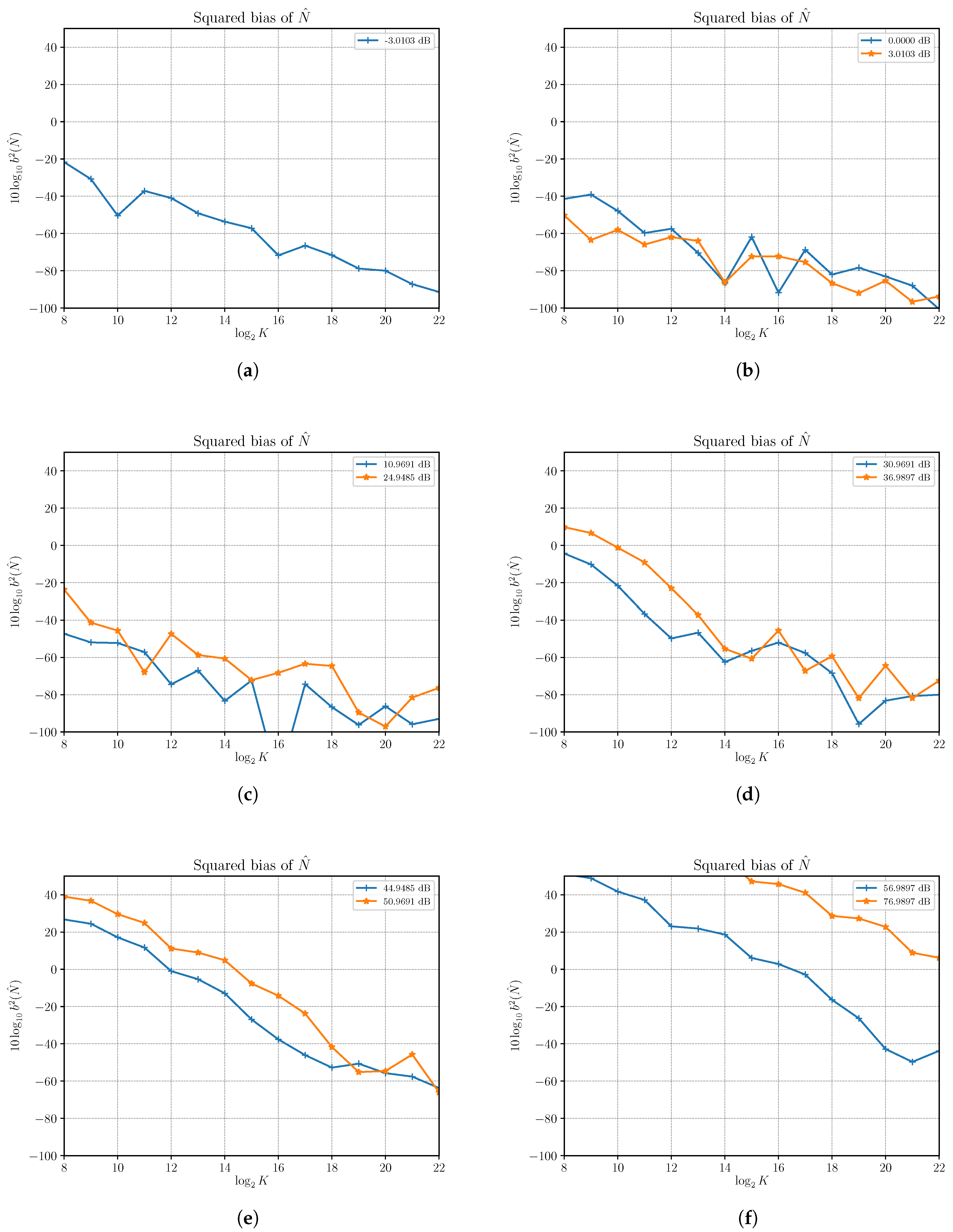
is asymptotically unbiased, as expected from first-order approximation analysis. Results of simulations run at different SNRs show that the estimated squared bias is very small even with a small number of observations. As an example, we report in
Figure 1 the estimated squared bias for
at different SNRs obtained by increasing
S and with
. Though the squared bias grows with increasing
S, and then with the SNR in this case, it can be made quickly very small by increasing the number of observed samples. Some bias is noticeable at high SNR; e.g., for 76.9897 dB with a low number of samples.
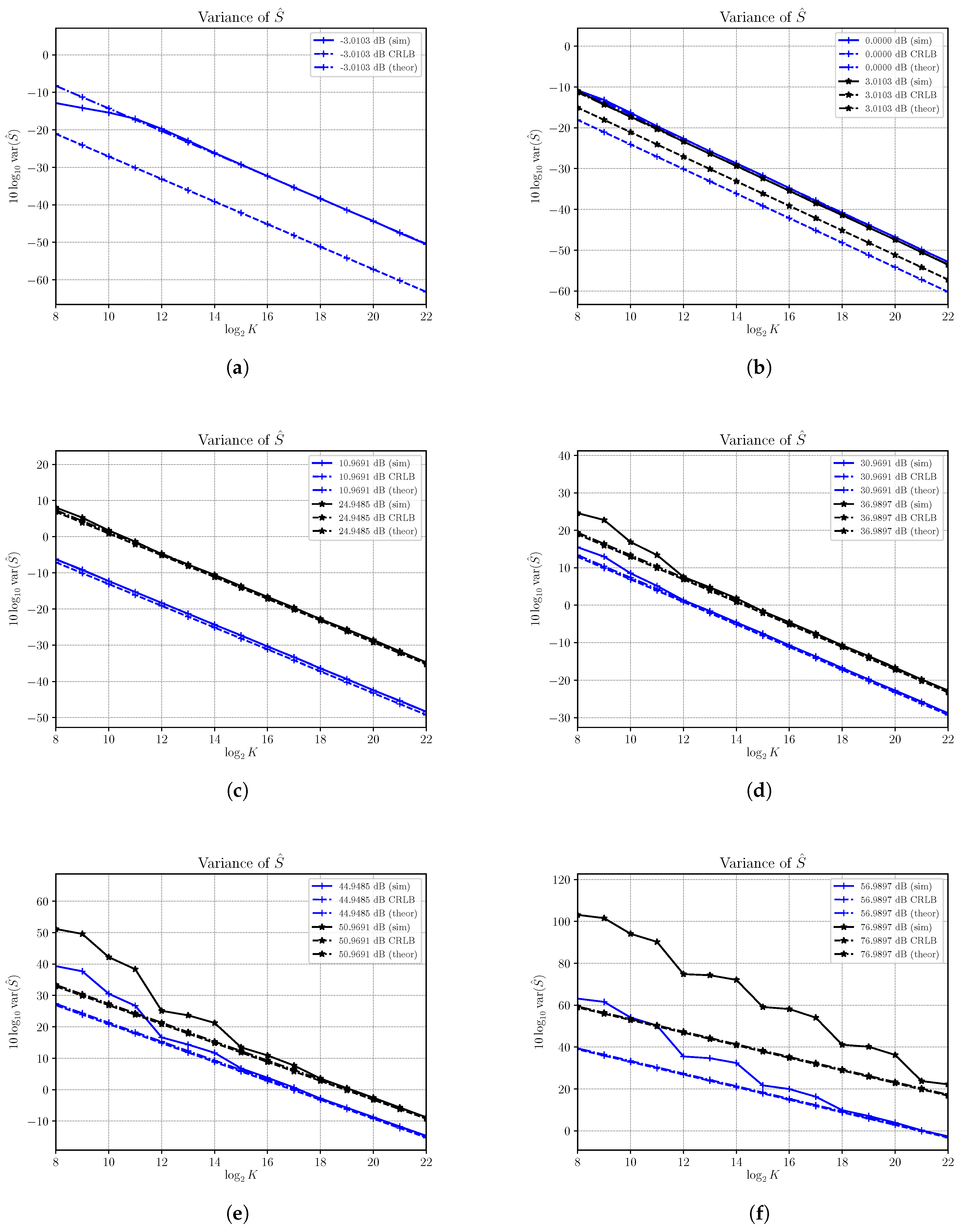
In
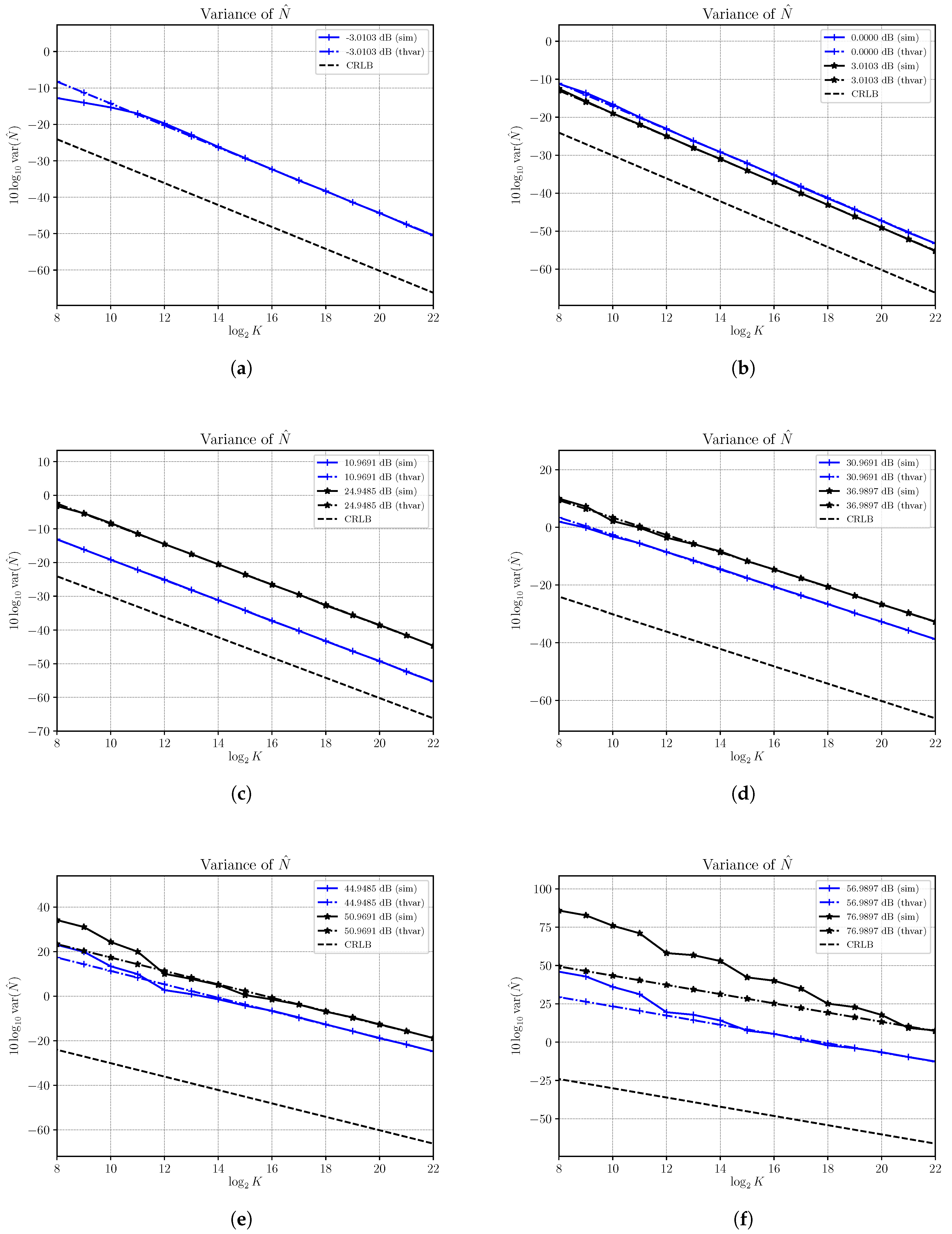
Figure 2 we show the results of estimated variance of the estimator
at different SNRs, denoted with (sim), and we compare the results with the corresponding CRLBs that we have derived in
Section 3 and asymptotic variances, denoted with (theor), derived in
Section 4. Variances are reported on a logarithmic scale as
versus the
, where
K is the number of observed samples.
We note that estimated variances reach the corresponding asymptotic performances in the whole range of SNRs under consideration, confirming the validity of the asymptotic performances derivation. However, the number of samples required to get the asymptotic performances depends on the current value of S: for low values of S, the estimator reaches quickly the asymptotic variance, while for high values of S the number of required sample results to be quite large. Unfortunately, it is not possible to predict when the asymptotic result is valid as the assumption made in performance derivation is to have a large number of samples.
Plots in
Figure 2 show also how the CRLBs for
depend on the current value of
S and become very high as
S increases. In general, the CRLB for
(
16) depends on the product
and then for fixed
N it becomes larger as
S increases; i.e., the best accuracy that can be obtained worsens with increasing signal power. On the other hand, the asymptotic variance depends on both
S and
N through terms of the type
, with
k and
m non negative integers, that are present in both the derivatives of the function that maps the moments to the estimate, i.e.,
, as defined in (
29), and its derivatives (
30) and (
31), and the covariance matrix (
26).
In
Figure 2a,b we see that for SNRs equal to
dB and
dB the estimator
is not asymptotically efficient though it is consistent, as the asymptotic variance and the corresponding CRLB are not superimposed. Note that the difference between the asymptotic variance and the CRLB, that cannot be filled by simply increasing the number of observations, can be calculated by means of the results derived in
Section 3 and
Section 4.
On the other hand, for higher values of S with , the asymptotic variance is superimposed to the corresponding CRLB, showing that for a large range of SNRs under consideration the estimator is efficient and that such efficiency is reached in many cases with a relatively small number of samples. However, as S increases the bound is reached for an increasing number of observed samples. For example, while with an SNR of 50.9691 dB we need at least samples to get the asymptotic behavior; at 76.9897 dB the estimated variance reaches the corresponding asymptotic variance with at least samples. For even higher S we expect that the number of samples required to get asymptotic performances to increase exponentially.
5.2. Performances of
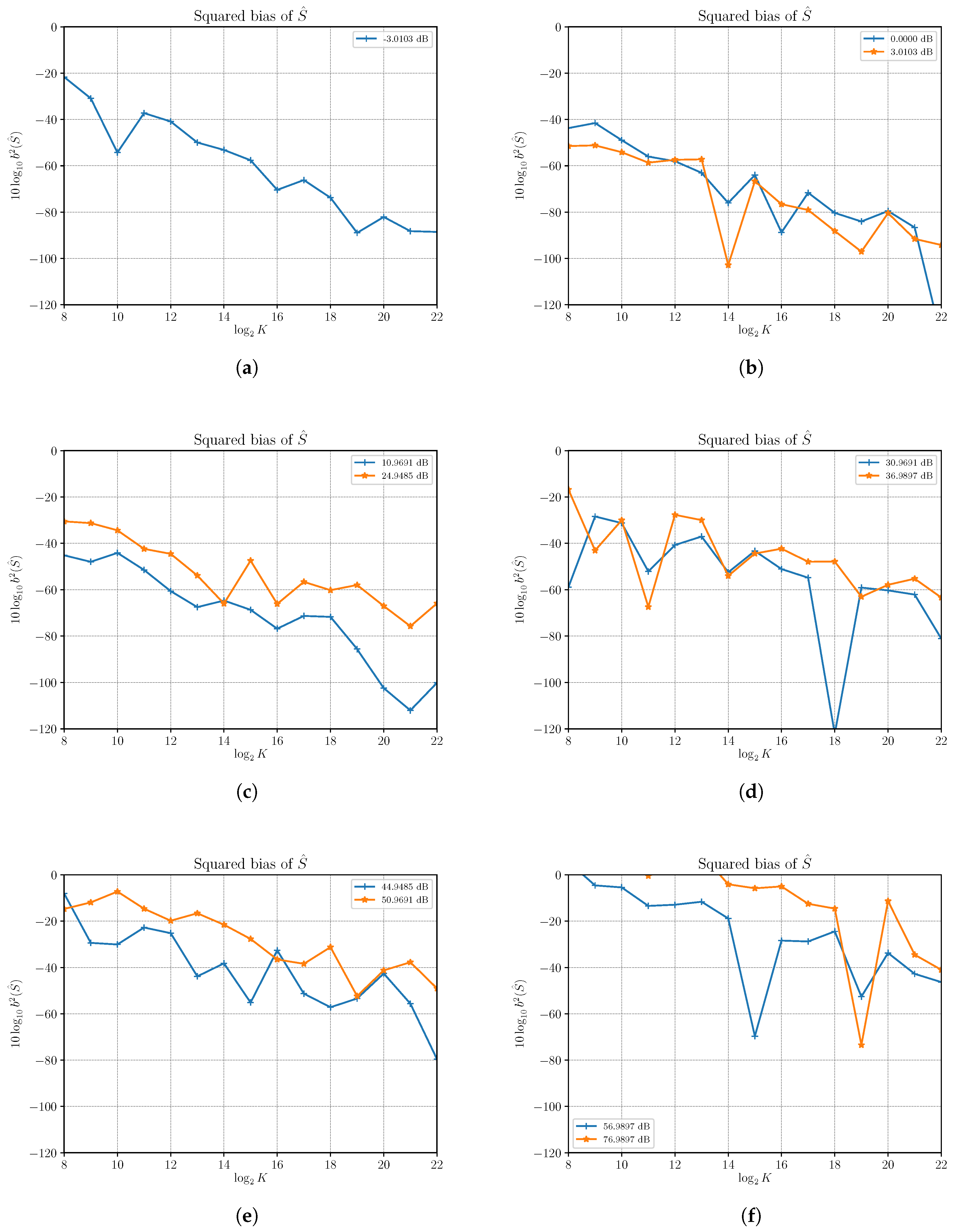
We verified that the estimator
is asymptotically unbiased. In fact,
Figure 3 shows that, for most of the SNRs taken into consideration obtained by changing
S with
, the estimator is practically unbiased even for small number of samples. For high SNRs the number of samples must be increased beyond
to get acceptable small squared bias; e.g., less than
.
In
Figure 4 the estimated variances, denoted with (sim), along with the corresponding asymptotic variances, denoted with (theor), and CRLBs, at different SNRs are shown. Note that the CRLB of
(
17) depends on
only and in the figures remains constant as, also in this case, the increase of the SNR is obtained by increasing
S while the noise power remains constant with
. Variances are reported on a logarithmic scale as
versus the
, where
K is the number of observed samples.
Results show that the estimated variance achieves the asymptotic performances for the whole range of SNRs into consideration. As for the case of the signal power estimation, it is not possible to predict the number of samples from which the asymptotic variance expresses the exact variance because the asymptotic analysis presented in
Section 4 is based on the fundamental assumption that
.
While the noise power estimator is asymptotically consistent in all cases, it is not efficient, since it cannot achieve the CRLB, in all cases under investigation. The difference between the asymptotic variance and the CRLB remains constant as the number of samples increases and depends on the current value of the signal power
S. In
Figure 4b we note that the difference decreases as
S increases; e.g., for a given
K the asymptotic variance of
with an SNR of 3.0103 dB is closer to the CRLB than the asymptotic variance of
at 0 dB. On the other hand, in
Figure 4c–f we see that the difference becomes lager and larger and asymptotic variances of the noise power estimator are quite faraway from the CRLB. In other words, though the estimator
is consistent, it may require too many samples to get acceptable performances. Moreover, it is not asymptotically efficient since the asymptotic variance is not superimposed to the corresponding CRLB.
5.3. Performances of
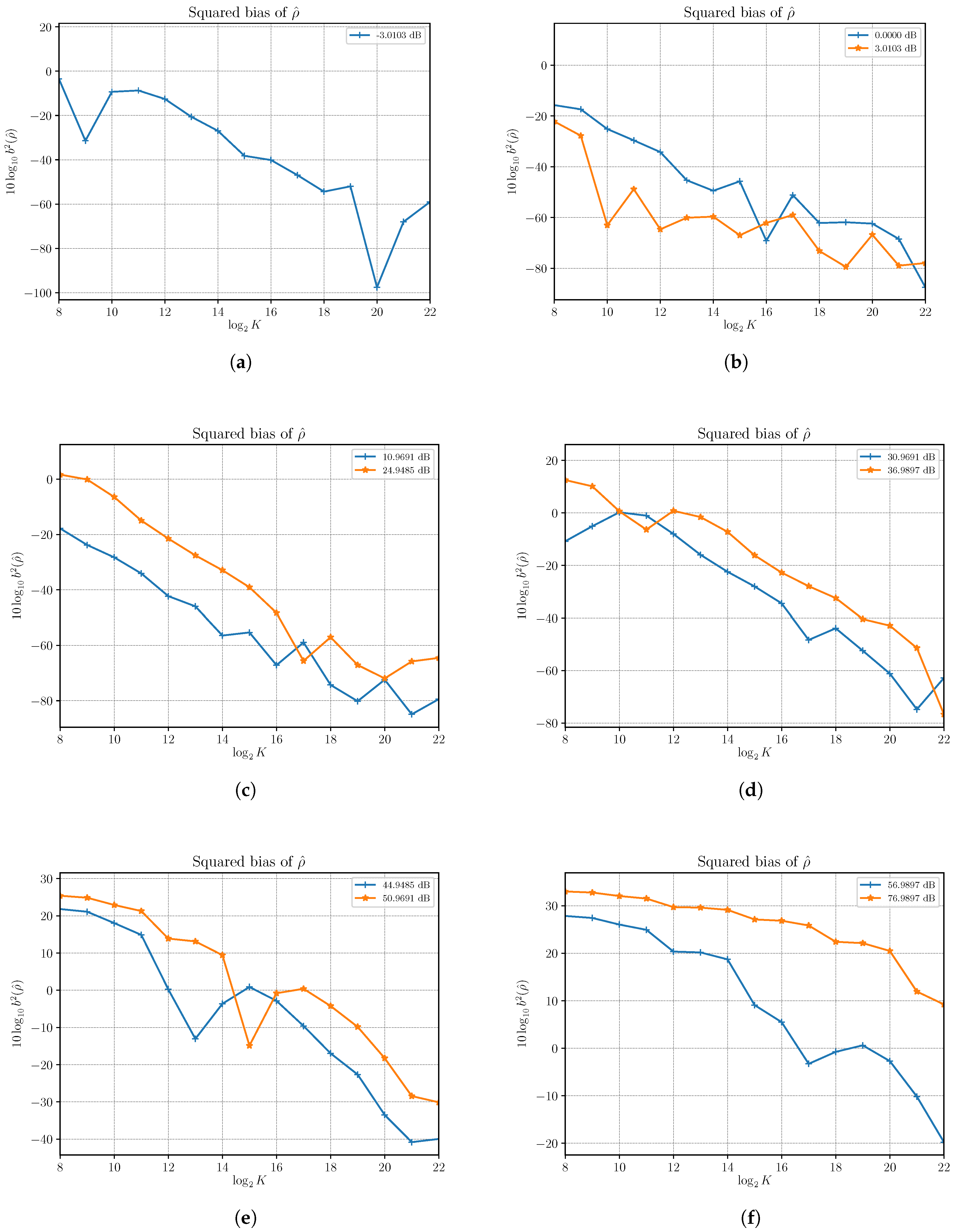
In
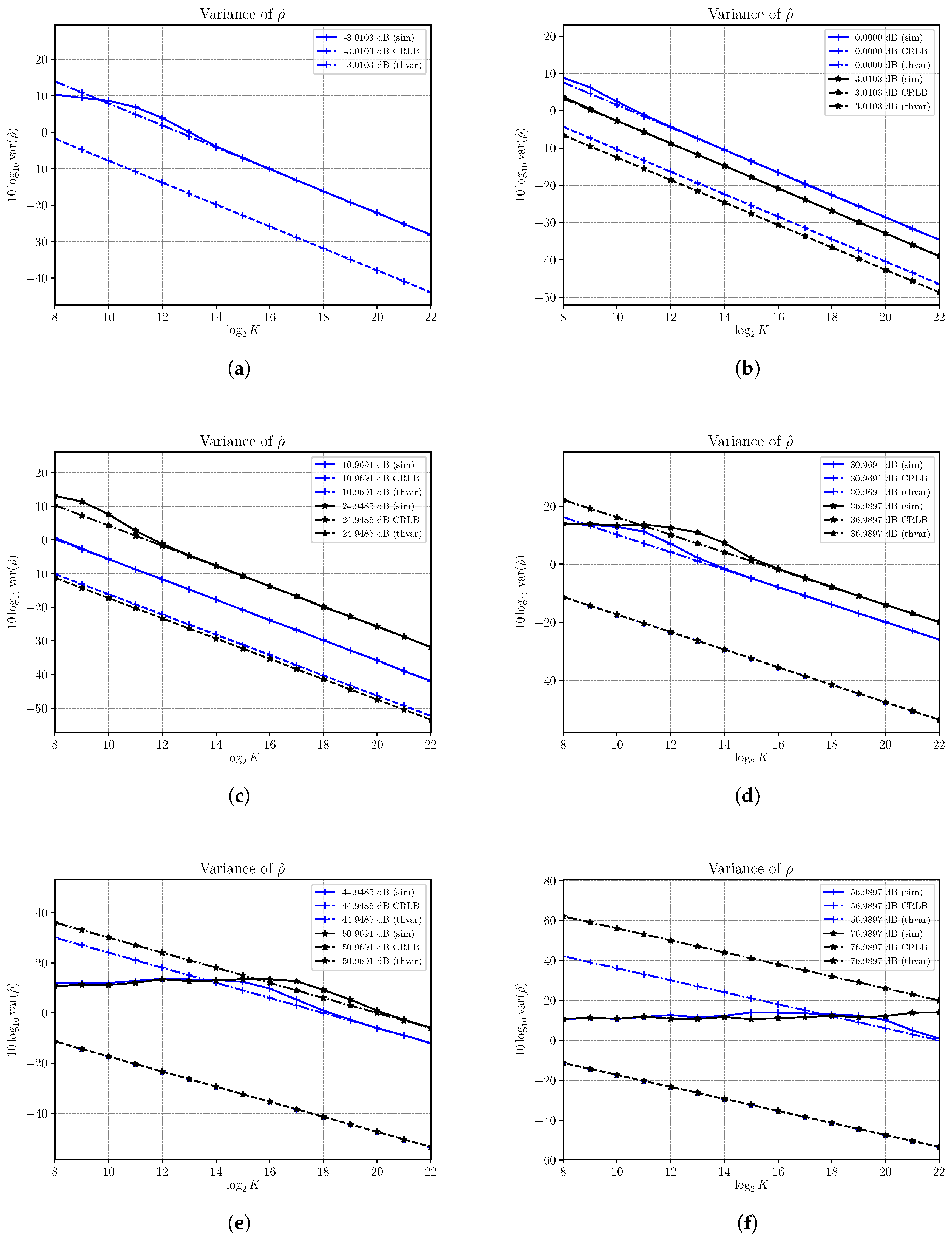
Figure 5 we show the estimated squared bias of the SNR estimator
as a function of the number of observations
K at different SNRs, obtained by changing
S with
. Results reveal that, in certain cases, the SNR estimator exhibits some bias that depends on both
S and
N to be estimated and the number of samples observed over which the estimate of the SNR is computed. In fact, for a sufficiently large number of observations, the squared bias can be made very small, even if that means that for high values of
S the number of observations required for an unbiased estimator is very large; e.g., with an SNR of 76.9897 dB the squared bias is still greater than one with
observations.
Estimated variances, denoted with (sim), at different SNRs as functions of the number of observations are shown in
Figure 6 where asymptotic variances, denoted with (theor) and corresponding CRLBs are also shown.
In
Figure 6a,b we show results for SNRs in the range from −3.0103 dB to 3.0103 dB obtained by varying
S with
. Within this range the SNR estimator becomes quickly unbiased and the asymptotic performances are reached for small sizes of observation windows. The SNR estimator is consistent but not efficient, as the estimator’s variance and the corresponding CRLB are not superimposed. We note that such a gap becomes smaller as S increases.
In
Figure 6c,d we show results for SNRs within the range from 10.9691 dB to 36.9897 dB. The estimated variances reach the corresponding asymptotic variances, though a greater number of samples is needed. In this case we see that the difference between the estimator’s variance and the corresponding CRLBs increases as
S increases. Note that as the SNR increases the dominant term in (
23) becomes
that does not depend on the SNR to be estimated, while estimator’s asymptotic variances given, in general, by (
24), and plotted in
Figure 6, still depend on
S and
N.
Performances degrades as
S increases with
. In
Figure 6e,f we consider increasing SNRs from 44.9485 dB to 76.9897 dB, a range for which the estimator is biased even for relatively large number of samples. The estimated variances reach the asymptotic performances only when the number of samples is high enough and the SNR estimator becomes substantially unbiased. For example, when the SNR is equal to 76.9897 dB and
we need more than
samples to get the asymptotic variance. Most importantly, for higher values of
S the asymptotic performances show that to get acceptable accuracies the number of samples must be increased even further.
6. Conclusions
It is possible to obtain with the method of moments, blind estimators for signal power, noise power and signal-to-noise ratio when a deterministic real sinusoid is corrupted by additive white Gaussian noise. We have derived new estimators by providing a general formula for the moments of the observed signal of any even order that is valid for a sufficiently large number of samples observed.
The performances of the proposed estimators have been studied through analytic derivation of asymptotic variances and Cramer–Rao lower bounds and confirmed through Monte-Carlo simulations. A general expression for the covariance matrix of the even-order sample moments has also been derived to get the asymptotic performances of the proposed estimators. Such an expression is valid asymptotically and can be useful to evaluate performances of any moment-based estimator for the same signal model, when a deterministic real sinusoid is corrupted by additive noise.
Analytical and numerical results show the estimator of signal power results to be asymptotically efficient and consistent for a large range of SNR values obtained by varying the signal power S and with . On the other hand, at low SNRs and with , below approximately 10 dB, the estimator is not efficient, though still consistent. Similar results have been obtained with the noise power estimator . The SNR estimator results were consistent in all the cases we studied. However, it is not efficient and we observed a performance degradation with respect to the corresponding CRLB that becomes larger as the signal power S increases and .
As a general consideration, we found that the performances can be acceptable in a relatively wide range of SNRs. However, since we have found that there exists a strong dependence between S and N to be estimated and the number of observations, special care in the choice of K is required when this estimator is used in practice to get acceptable performances. Numerical examples show that in some cases the SNR estimator has very good performances and then it can be used to obtain an accuracy very close to the CRLB. The asymptotic results presented in this paper represent a useful mathematical tool that may provide useful guidance to expected performances before any practical implementation, letting any practitioner assess the performances, and then, usefulness, of the proposed estimators based on his application needs and operating conditions.

