Article

A Comparison of Energy Management System for a DC Microgrid

by
Luis O. Polanco Vásquez
1,
Víctor M. Ramírez
1,* and
Kary Thanapalan
2
1
Unidad de Energía Renovable, Centro de Investigación Científica de Yucatán AC., Mérida CO 97200, Yucatán, Mexico
2
Faculty of Computing, Engineering and Science, University of South Wales, Pontypridd CF37 1DL, UK
*
Author to whom correspondence should be addressed.
Appl. Sci. 2020, 10(3), 1071; https://doi.org/10.3390/app10031071
Submission received: 9 January 2020 / Revised: 29 January 2020 / Accepted: 31 January 2020 / Published: 5 February 2020
(This article belongs to the Special Issue Microgrids II)

Abstract

:
This paper investigates the analysis of the energy management system for a DC microgrid. The microgrid consists of a photovoltaic panel and a batteries system that is connected to the microgrid through a bidirectional power converter. The optimization problem is solved by the hybrid internal point method with the genetic algorithms method and particle swarm optimization (PSO) method, by considering forecasting demand and generation for all the elements of the microgrid. The analysis includes a comparison of energy optimization of the microgrid for solar radiation data from two areas of the world and a comparison the efficiency and effectiveness of optimization methods. The efficiency of the algorithm for energy optimization is verified and analyzed through experimental data. The results obtained show that the optimization algorithm can intelligently handle the energy flows to store the largest amount in the batteries and thus have the least amount of charge and discharge cycles for the battery and prolong the useful life.

1. Introduction

During the last two decades the development of energy management systems (EMSs) has been of interest by the energy research community. This interest is due to the continued and improved development of renewable energy systems (RE), and the EMS optimization techniques with advanced energy storage systems [1].
The efficient use of energy in any field has become paramount due to environmental, economic and operational aspects, therefore, the study of energy management in a microgrid is vital [2]. Microgrid can be classified according to their operation in autonomous and non-autonomous, the use of an autonomous microgrid can be seen in rural areas and in the use of equipment that needs energy autonomy for their operation as space vehicles or other sea vehicles where it cannot connect to the power distribution grid [3]. The non-autonomous grid can be seen in the residential, industrial grid and currently it is also connected to a general energy distribution grid either to export or import energy for many different applications [4]. However, the efficient use of the microgrid is difficult due to the presence of distributed energy resources, which can be controllable (or dispatchable), such as gas turbines or diesel engines, but also not controllable (or non-dispatchable), such as wind turbines or photovoltaic (PV) generators. Tidal generators whose production depends largely on weather conditions, which in turn can be predicted for long periods of time with some uncertainty [4]. Microgrids contribute to the preservation of the environment and energy sustainability as they reduce losses in the distribution lines and also mitigate the expansion of the main network and can be used to provide electricity to rural areas, space vehicles and autonomous sea vehicles and many other applications [5].
Wang et al. [6] conducted a comparative study of the different energy management strategies and examined the operation modes via simulation studies.
Zia et al. [7] presents a comparative and critical analysis on decision making strategies and their solution methods for microgrid energy management systems. To manage the volatility and intermittency of renewable energy resources and load demand, various uncertainty quantification methods are summarized. A comparative analysis on communication technologies is also discussed for cost-effective implementation of microgrid energy management systems. Finally, insights into future directions and real-world applications are provided. An overview of the DC microgrid system and the estimation of the energy savings of the DC microgrid over conventional AC systems are described in [8]. The study examined the system performance in locations across the United States for several commercial building types and operating profiles. It is found that the DC microgrid uses generated PV energy 6%–8% more efficiently than traditional AC systems.
Zafar et al. [9] presents a comparative study of different optimization techniques, the genetic algorithm, the pattern search method and the interior point algorithm are used to optimally schedule the energy required from the thermal power generators to meet the load demand by taking into account the power from the renewable energy resource, a comparison of the optimal cost values that each optimization method obtained is made, the emission comparison is also performed and finally the time i uses to converge each method. In [10] the author illustrates the utilization of the particle swarm optimization (PSO) method for cost-efficient energy management in multi-source renewable energy microgrids. PSO algorithm is used to find out optimal energy mixing rates that can minimize daily energy cost of a renewable microgrids under energy balance and ant islanding constraints. The optimal energy mixing rates can be used by multi-pulse width modulation (M-PWM) energy mixer units, the methodology analyzed is TRM-PWM that is a pulse wide modulated switching method that can mix energy flow from various energy sources by allocating pulse wide duration at different time rates for several sources [11]. Askarzadeh et al. [12] proposes a memory-based genetic algorithm (MGA) that optimally shares the power generation task among a number of Distributed Energy Resources (DERs). The MGA is utilized for minimization of the energy production cost in the smart grid framework. It shares optimally the power generation in a microgrid including wind plants, photovoltaic plants and a combined heat and power system. In order to evaluate the performance of the proposed approach, the results obtained by the MGA are compared with the results found by a genetic algorithm and two variants of particle swarm optimization. Simulation results accentuate the superiority of the proposed MGA technique.
This paper presents a unified model of EMS for microgrids, which considers basic models of the elements of the photovoltaic panels, batteries for the energy storage system, as well as the geometric model of solar radiation. The model is solved by means of the hybrid internal point method and genetic algorithm (IP-GA) and particle swarm optimization (PSO) method provided by the MATLAB® optimization toolbox [13]. The solution of this model then allows us to evaluate the optimal management of energy storage devices. In addition to the geometric model of solar radiation, it is possible to evaluate the impact of the solar resource on energy management in that of storage systems. The analysis of optimal use of the storage system is illustrated by means of a numerical example, which considers a microgrid of four nodes.
The main novelty of this work is that the difference of the works presented in the introduction paragraph where only one optimization method is presented in this document presents two different optimization methods for EMS that has results obtained for energy optimization, also in this work, as it is proposed under the concept of day ahead, it uses the power balance and inequality constraint equations to maintain the power and voltage levels of all the elements of the microgrid obtaining adequate operational results of the affected variables.
The paper is organized as follows: Section 2 presents the models mathematical of the different components of the microgrid, this section describes the model mathematical of the photovoltaic system, the storage system (battery), the electric load and the geometric model of global radiation on an arbitrarily inclined surface. Section 3 describes the general and specific optimization model, in this section the models of the microgrid components are unified into a single model. In addition, the EMS algorithm for the microgrid is based on the equations of the unified microgrid model. Section 4 shows the results obtained from the simulation of the unified microgrid model, where the power levels generated by the microgrid sources are shown, the voltage levels in the nodes, the comparison of fitness value and computation time are observed of the optimization methods. Section 5 presents the conclusions of the paper.

2. Mathematical Modeling for DC Microgrid Components

In this section mathematical models developed for the components that set up the micro-grid and the main electrical system are presented in order to achieve an adequate coupling with the electrical devices (solar panels and storage system such as a battery bank), in which the control actions will be carried out. This leads to the development of a complete mathematical model of the micro-network and the electrical system.

2.1. Batteries

The battery banks are one of the main energy storage systems and it can be used to store energy from renewable generation sources connected to the microgrid. Unlike renewable sources of generation, these elements can be considered as dispatchable energy sources because stored energy can be used in a controlled manner. The battery pack can function in the charge or discharge mode to give or absorb a net amount of active energy, at their connection point. This allows us to manage the level of energy stored in them. The level of stored energy is reflected through the state of charge (SOC). Considering that the bank is made up of j, the j-th battery can then be represented by means of two active power generation sources, as illustrated in Figure 1 [5]. One of them represents the charging power of the j battery at a stage i of time t, and the other the discharge power of the j battery at a stage i of time t, the sum of both powers represents the net power of the j battery in a stage i of time t that belongs to a set of stages, contributed or consumed by the battery in its connection node.
p S n j t i = p S c j t i + p S d j t i ; 0 p S d j t i ;   p S c j t i 0 ; t i T
The decision variables the storage system are V j t i and [ p S d j t i , p S c j t i ] x S   ( t i T ) being xS the batteries variables, while [ V j t i ] x R   ( t i T ) The state of charge (SOC) of the j battery in the stage ti S O C S   j t i can be calculated by means of Equation (2).
s o c s j t i = s o c S j t 0 ε c j Δ t E S n o m   j t = 1 t i p S c j t Δ t E S n o m   j ε d j t = 1 t i p S d j t

2.2. Photovoltaic Modules

The commonly used solar PV cell model is a single diode model is shown in Figure 2 [14]. The module is connected to a micro-grid point through Buck-Boost DC–DC converter. The expression in Equation (3) represents the mathematical behavior of the current in module terminals I C D k t i [15]. Where the meaning of each term is as follows: the current of the photovoltaic module is represented by I P V , The current of saturation is represented by I S , the DC voltage in the module terminals represented by V CD   k t i , the resistance in series is represented by R S , the number of cells connected in series represented by n s and the number of cell connected in parallel represented by n p . The term R S is evaluated from Equation (4), where the open circuit voltage represented by V o c , the voltage of the point of maximum power represented by V m p p t , the current of short circuit electricity represented by I S C , the current maximum power point electricity represented by I m p p t . Mathematical expression of I S C must also be evaluated through Equation (5). Where the current short circuit electricity standard under the conditions of test represented by I S C , s t c , irradiance represented by G , irradiance under the test represented by G s t c , electricity temperature coefficient represented by k l , temperature of the panel represented by , standard temperature under the test of the panel represented by T s t c V o c are evaluated through Equation (6) where standard low open circuit voltage conditions test is represented by V o c , s t c and temperature coefficient represented by k v [16].
I C D k t z = [ I P V I S ( e x p ( V C D k t i n s + I C D k t i n p R S V C D t i ) 1 ) ] n p ; t i T
R S = V o c V m p p t n s + V C D t i ln ( I S C I m p p t I S C ) I m p p t n p
I S C ( T , G ) = I S C , s t c G G s t c [ 1 + k l 100 ( T s t c ) ]
V o c ( T ) = V o c , s t c [ 1 + k v 100 ( T s t c ) ]
In this paper, the photovoltaic module parameters involved in Equations (3)–(6) were obtained from the features of the monocrystalline module brand Silfab model SLAM 300 [17].
Equation (7) describes the power generated in DC terminals of the photovoltaic module to the microgrid.
p C D k t i ( V C D k t i , I C D k t i ) = I C D k t i V C D k t i ; t i T

2.3. Electrical Load

The load characteristics selected for the analysis of the EMS applied to a solar system were based on a relatively small (10.4 m, 6.085 m) two storage office block. Solar power was used to supply the load demand. The system should utilize excess solar power to store the energy in the battery bank. The load profile is represented by a model of constant power for any interval of time T. The power i-th p l m t i active consumed in the node is then represented by Equation (8) where p l m t i represent the power consumption active on that node at the instant ti [18].
p l m t i ; t i T
The only decision variable that introduces the constant power model to the optimization problem is the magnitude V i t i of the connection node, such as [ V i t z ] x R ( t z T ) .

2.4. Solar Radiation

The solar radiation incident on the panel is modeled to have a better estimate of the energy production of the photovoltaic panel so that the EMS performs correct optimization. Radiation is a parameter that depends on many variables, both temporal and position, therefore, its modeling is somewhat more complex than the panel model. To model the incident solar radiation will have to be characterized from the equations that govern the behavior of radiation on an inclined surface [19].
The global irradiance G ( α , β ) on an arbitrarily oriented and inclined surface: It is calculated with the components of direct irradiance on an inclined B ( α , β ) , irradiance diffused D ( α , β ) , and irradiance reflected R ( α , β ) plane, as shown in Equation (9).
G ( α , β ) = B ( α , β ) + D ( α , β ) + R ( α , β )
Direct radiation on an arbitrarily oriented and inclined surface B(α,β) is calculated through the direct radiation measured on a horizontal surface B ( 0 ) and the geometric terms such as angle of incidence ϑ S and the angle or zenith distance ϑ Z S , as shown in Equation (10).
B ( α , β ) = B ( 0 ) c o s ϑ S c o s ϑ Z S
Radiation reflected on arbitrarily oriented and inclined surface R(α,β) is calculated through the reflected radiation measured on horizontal surface R ( 0 ) and the geometric terms such as the angle of inclination β , as shown in Equation (11).
R ( α , β ) = R ( 0 ) ( 1 c o s β 2 )
Diffuse radiation on an arbitrarily oriented and inclined surface D(α,β) is calculated through the reflected radiation measured on a horizontal surface R ( 0 ) , the geometric terms such as the direct irradiance transmission index A i and others mentioned in the previous paragraphs, as shown in Equation (12).
D ( α , β ) = D ( 0 ) ( 1 c o s β 2 ) ( 1 A i ) + D ( 0 ) c o s ϑ S c o s ϑ Z S A i

3. DC Microgrid Model

The general model of the microgrid is posed as a problem of optimization. The optimization model [20] is given by Equations (13)–(16). It should be noted that, in this model, it is considered that the period of time T is composed of a set of time stages tz (∀= 1,…, end), such that T= (t1,…, tend).
Minimize   F T =   t i = 1 t e n d f t i ( x t i )
S u b j e c t   t o   n t i ( x t i ) = 0 ;   t i T
z t i ( x t i ) 0 ;   t i T
x _ x t i x ¯ ; t i T
The terms of the optimization model are as follows: the objective function F T to be optimized in stage i of the time interval T, n t i ( x t i ) represents the set of equality constrains that are raised as the power balance equations in all the connection nodes of the microgrid, as well as other operating conditions that must be fulfilled unconditionally, z t i ( x t i ) is a set of constraints of inequalities that represent the maximum and minimum values that can be physically taken by the different renewable energy sources that form the microgrid, x is the set of variables to optimize for energy management composed of subsets x R t i , x p v t i and x S t i such x = [ x R t i , x p v t i , x S t i ]. Where, x S t i , x R t i and x p v t i represent batteries variables, microgrid and photovoltaic modules, respectively. These decision variables are specified for each element of the microgrid in the final part of the specific model of the DC microgrid section. The upper and lower limits, x ¯ and x _ , of these variables are formulated through the inequality constraints, see in Equation (16). The physical values of the limits of these variables are specified in Appendix A and Table A1.

3.1. Specific Model of the DC Microgrid

The specific model of the DC microgrid is explicitly formulated in this section for an autonomous DC microgrid. For this purpose, the objective function is expressed in extended form in the Equation (17).
F T = t z = 1 t e n d j = 1 N p c c a j + b j ( p R j t i ) + c j ( p R j t i ) 2
Note that Equation (17) denotes that the objective is to minimize the cost of the total energy photovoltaic system during the period of time T to supply the demand curves predicted p l m t i m , t i T .
The set of equality constraints n(x) is expressed in Equation (14) and correspond to the equations of the active power balance of the nodes of the DC microgrid Δ P R i t i 
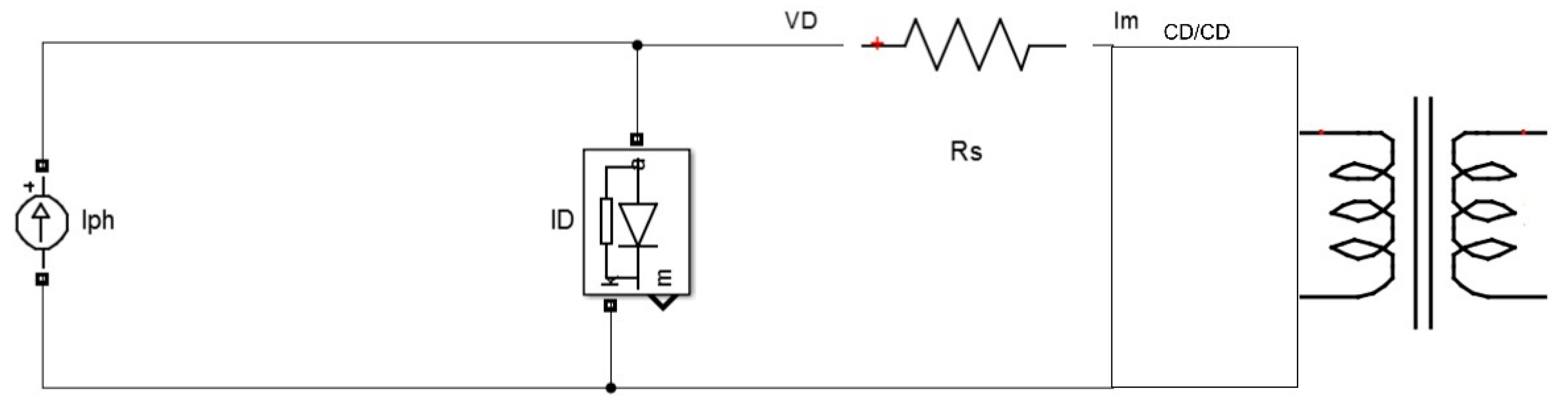
, these constraints are written in the first block of Equation (18) where the lower limit ∀jm means each element j is connected to the node m. For example, in this block we have the sum of the charge p S c j t i and discharge powers p S d j t i of the storage system, the sum of the power of the photovoltaic panel p p v j t i and the powers injected p l j t i into the nodes of the microgrid. In the third block of Equation (18) is expressed the equations of active power balance in node of photovoltaic panel Δ p C D k t i [9].
n t i ( x t i ) = { 0 = j m p S c j t i + j m p S d j t i + j m p p v j t i j m p l j t i Δ I C D k t i = I C D k t i f C D ( V C D k t i , I C D k t i ) = 0 , Δ p C D k t i = p C D k t i ( V , I ) Δ p C D k t i ( V C D k t i , I C D k t i ) = 0 , }   t i T
The only inequality constraints function z(x) introduced in the optimization problem are those due to the storage system, because the batteries have finite charge and discharge capacity that can vary between a minimum of 20% and a maximum of 100% depending on the battery material. Therefore, the SOC is modulated over the period T through Equation (19) [21].
z t i ( x t i ) = { s o c S j m i n s o c S j t i s o c S j m a x }   j t i T
The inequality constraints variable x is set up of the set decision variables that must have admissible values for the operation of the microgrid. The decision variables must be limited to appropriate values throughout the time interval T, the inequality constraints variable is expressed in Equation (20).
{ x _ R x R t i x ¯ R x _ p v x p v t i x ¯ p v x _ S x S t i x ¯ S }   t i T
The microgrid has a set of decision variables associated with each node, which are the magnitude of the voltage as well as the powers exchanged with the different energy sources, such as x R = [ V j t i ,   p R   j t i ] ; t i T , whereas the decision variables batteries are x S = [ V sj t i , s o c s j t i , p Sd   k t i , p Sc   k t i ] t i T . Finally, the photovoltaic modules decision variables are x pv = [ V CD   i , t i I CD ,   t i p C D k t i ] ; t i T .

3.2. Algorithms

The algorithms described in this paper are composed of the genetic algorithm and interior point methods and PSO method. The first algorithm is applied through of the ga function, which belongs to the MATLAB® ‘Direct Search and Genetic Algorithm Toolbox’ and is especially useful for the optimization of global non-linear problems with or without constraints. Furthermore, it provides a better flexibility since it contains multiple parameters of configuration [13,22].
The ga function suggested specifies the values of the arguments of the set of inputs IA and outputs OA that are established and regulated for its execution. The general form of this function is shown in Equation (21).
[ O A ] = g a ( I A )
The second algorithm is applied through the PSO function, which belongs to the MATLAB® ‘Particle Swarm Toolbox’ and is especially useful for the optimization of global non-linear problems with or without constraints. Furthermore, it provides a better flexibility since it contains multiple parameters of configuration [13].
[ O A ] = p a r t i c l e s w a r m ( I A )
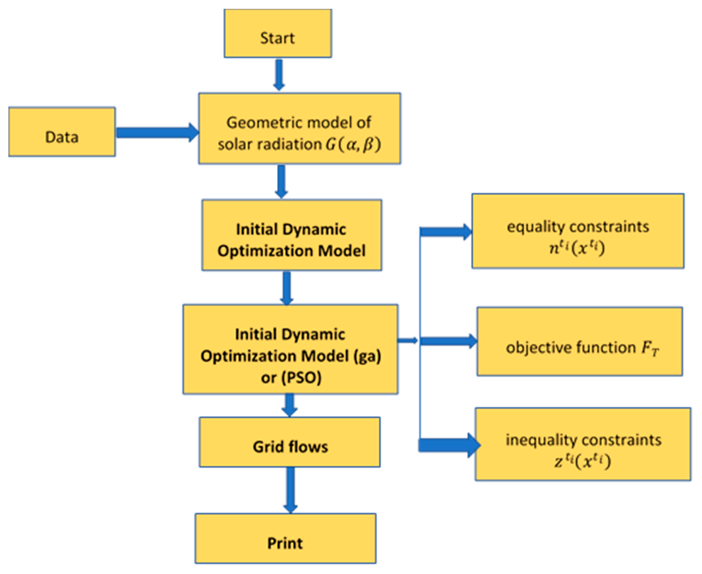
The description of the implementation of the algorithms is summarized by means of the represented algorithm in Figure 3.

4. Results

The results obtained numerically through a simulation carried out with a test microgrid, which is integrated by a photovoltaic system (PV), storage system (S) and the load (L). The data that were used for the test microgrid are real and also with these data the global irradiance on an arbitrarily oriented and inclined surface was calculated, a global irradiance profile of Cancun city (Mexico) and Baglan (Wales, UK) to make the comparison of the energy generation of the photovoltaic solar system for two different places in the world. The load profile used is the real data obtained from the Baglan Energy Park, Port Talbot, United Kingdom.
The results present the numerical values of the geometric model of solar radiation from the two cities mentioned above. It also presents the results of the behavior of the photovoltaic solar system and the storage system within the microgrid resolved through hybrid IP-GA method and PSO method, the methods to solve the optimization problem is determined in a PC DELL, with 8 GB RAM and an Intel i5-4210U CPU@ 2.40 GHz processor. The characteristics of the computer directly influence the speed in which the optimization algorithm can be solved.
In this work, solar radiation data from two different places in the world are compared to verify the behavior of the EMS considering the solar resource of each place evaluated. The load profile is based on a relatively small (64 m2) two store office block, which in fact forms part of a facility called the Hydrogen Center (University of Glamorgan at Baglan Energy Park, Port Talbot, United Kingdom).
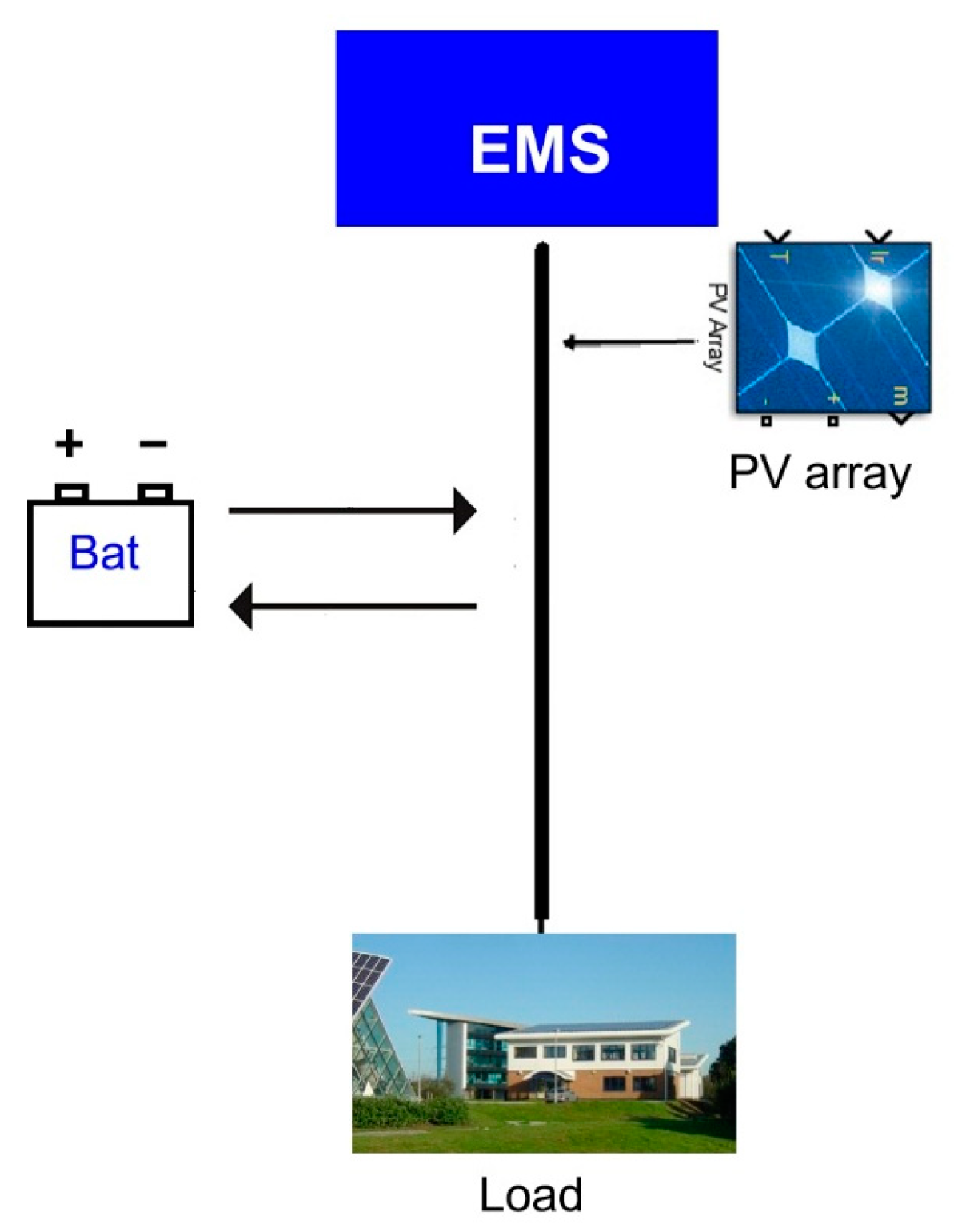
The microgrid test is shown in Figure 4. The values of the parameters of the different models of the microgrid are presented in Appendix A.
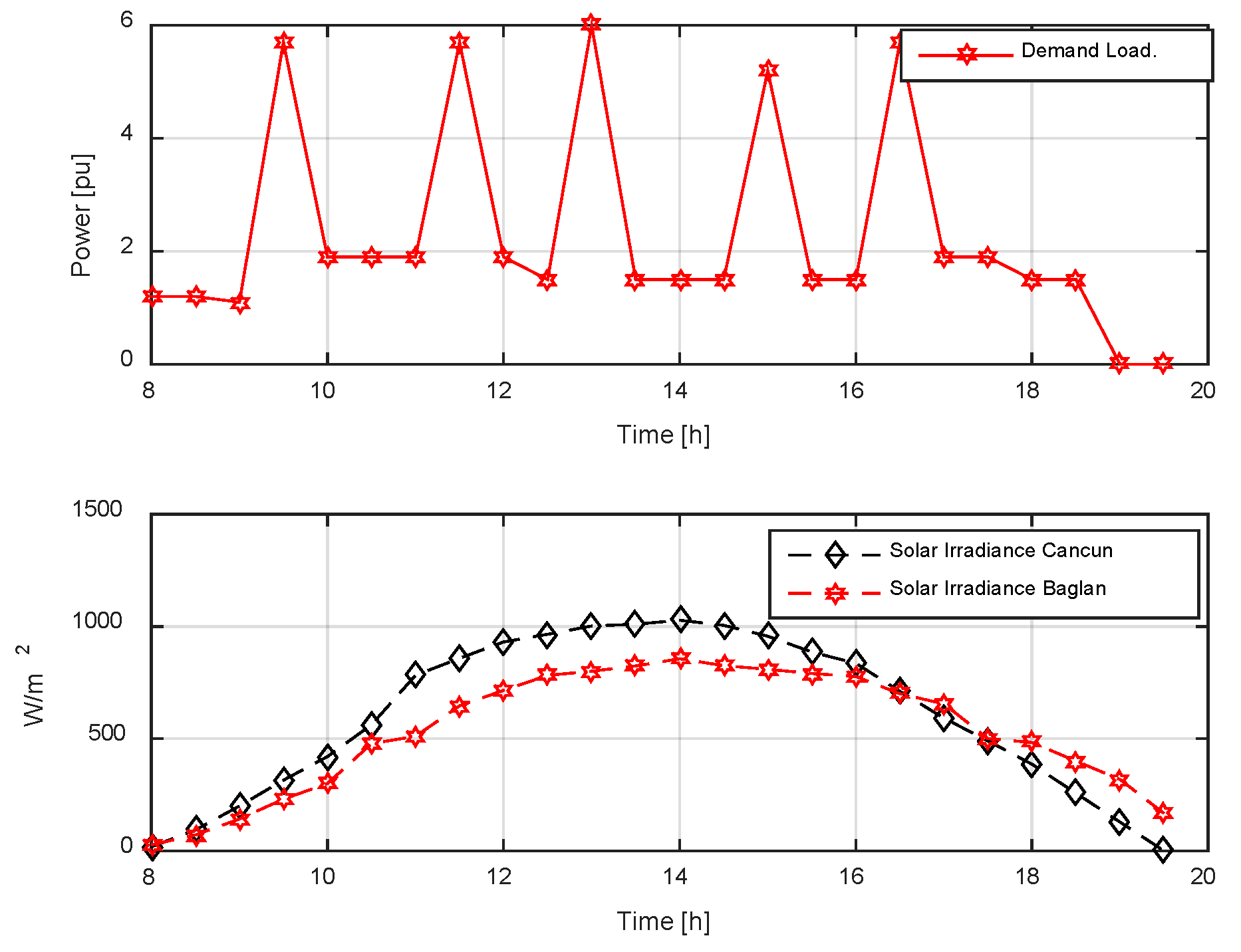
Comparative load and irradiation profile for a clear day (summer) for both cities are observed in Figure 5. The power and voltage bases were selected in 10 kW and 24 V, respectively.
The limits of the magnitudes of the microgrid are 0.92 V 1.05 per unit. The SOC limits on the battery are 0.2   s o c S ( t i ) 1   ( % ) , whilst the initial condition of the battery charge is s o c S ( t 0 ) = 0.6   ( % ) .
The EMS was developed with the genetic algorithm method with interior point hybrid (IP-GA) provided by the ga-fmincon function developed by MATLAB®. 
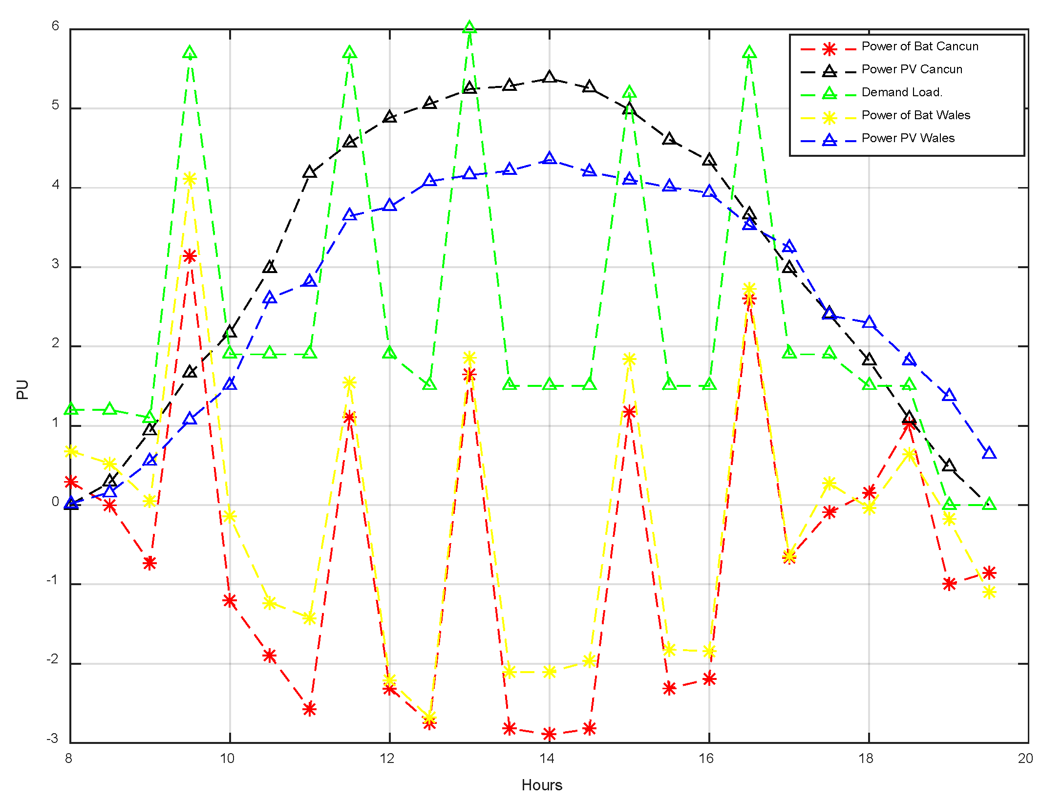
Figure 6 shows the comparison of the active power supplied by the photovoltaic panel and the battery for the two solar radiation conditions of a clean summer day in Cancun and Baglan. This figure shows that between the stages 8–20 h a demand profile is presented in the office block. In the demand that ranges between 1 and 6 KW, it is observed that the demand peaks occur at 9:30, 11:30, 13, 15 and 17 h.
The power supplies by the photovoltaic panel are not enough to supply the load demand, making it necessary to use the energy stored in the batteries to satisfy the load demand and avoid problems within the microgrid.
It can be observed, that the batteries take advantage of charging at times where the demand for the charge is minimal, such as in 9, 11, 12:30, 14, 15:45 and 17 h. This way it is possible to verify that the EMS algorithm works correctly. Furthermore, it was also observed from the two generation curves of the photovoltaic panel where the generation curve for the Cancun city shows a greater amount of energy than the Baglan city curve, due to the geographical position of each city.
Figure 6 indicates the active power supplied by the batteries. It is important to understand that the energy supplied by the batteries in the region of Cancun is less than that supplied in Baglan and it can also be seen that the batteries are charged with more energy in the city of Cancun since in this city the photovoltaic panel produces more energy for the largest amount of solar resources in the region.
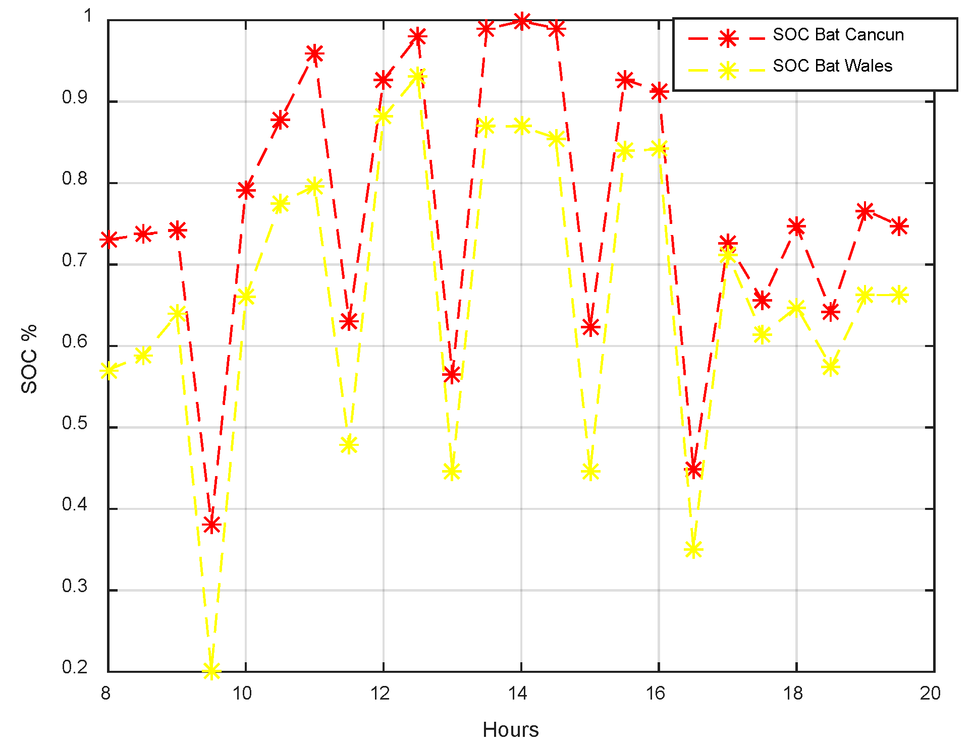
Figure 7 shows the SOC of the battery in yellow for the city of Baglan and in red the behavior in the city of Cancun. The results show that the SOC of the battery is consistent with the behavior of the battery charge and discharge graph of Figure 6. We could observe that at all hours of time the SOC of the battery in Cancun was higher due to the production of PV power in this city being greater due to the available solar radiation and therefore there was an opportunity to charge the battery more. For example, from 8:00 a.m. to 10:00 a.m. the battery in Cancun has a higher SOC the behavior was very similar from 10:00 a.m. to 4:00 p.m. at 5:00 p.m. the battery in Baglan managed to have an SOC similar to the battery of Cancun since at this time the production of PV in Baglan was greater. For the discharge we observed that at 9:30 a.m. the battery in Baglan is discharged to the maximum possible 20% while in Cancun the battery is discharged at 40%, this behavior is similar at 11:30, 13:00, 15:00 and 16:30.
This comparison shows us that having a greater availability of solar radiation the battery in an isolated micro network has less wear due to the lower number of use cycles.
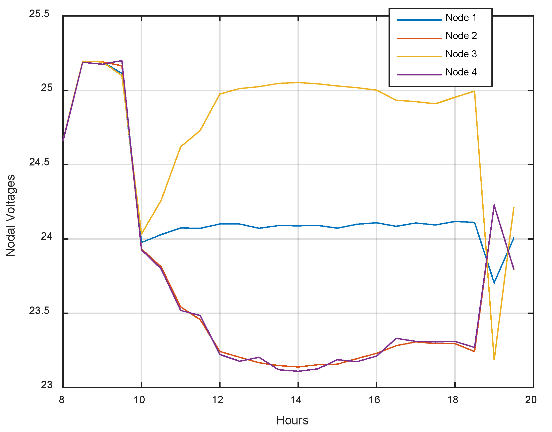
In Figure 8 shows the behavior of the nodal voltages within the microgrid. It is observed that the voltage levels were maintained in the minimum and maximum permissible values of 95%–105%, in this way it was verified that the inequality constraints to variable were preserved.
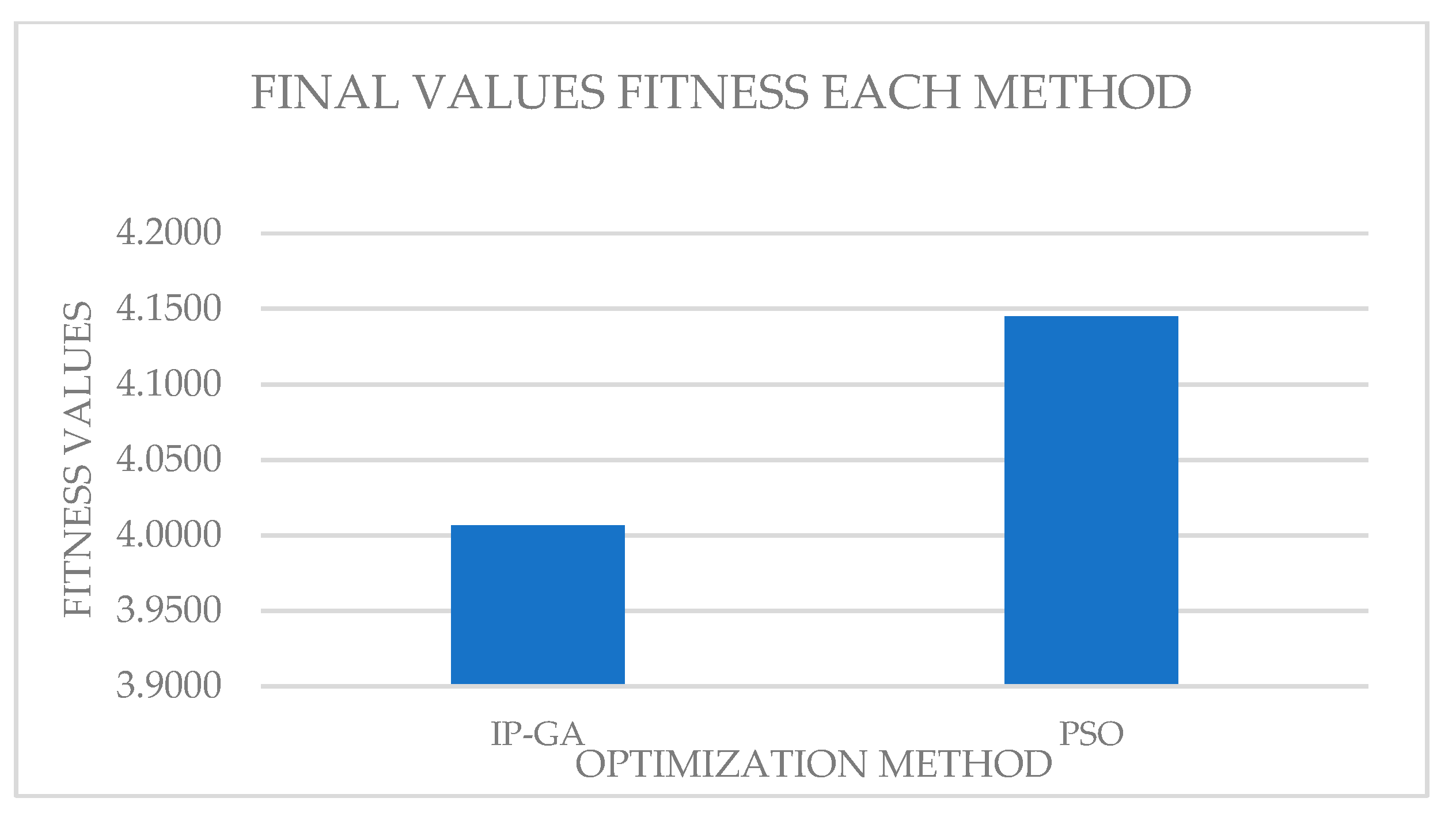
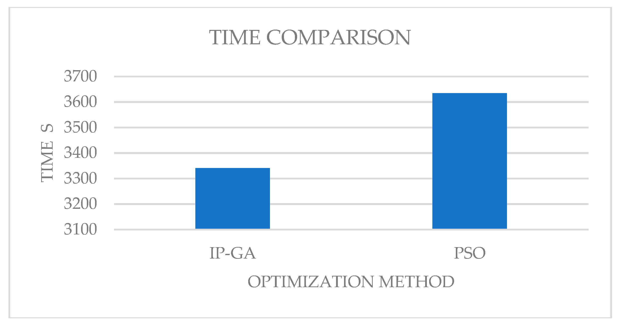
Figure 9 shows that the two methods IP-GA and PSO, the IP-GA method gave a better fitness value than the PSO method. The IP-GA was faster than PSO, reducing the computing time about 300 seg. as the Figure 10 shows.
Although the GA-IP was faster, the two methods used to solve the optimization problem in the microgrid could be considered like an effective method to solve the optimization problem and worked like a tertiary control within the microgrid. This is possible due the energy cost from the battery for the optimization methods being the most expensive for all times.

5. Conclusions

The results obtained from the EMS algorithm for the test microgrid were shown in this paper, a comparison of the solar radiation resources from two different places in the world was also made for a clear summer day. The two-optimization methods IP-GA and PSO were compared. The results show that the most effective method was IP-GA giving a better fitness value and taking less time to solve the optimization problem, but the PSO method shows an acceptable solution for the optimization problem and became another alternative for EMS in the microgrid. The solar radiation comparison showed that for Cancun city, due to its geographical position, had a better solar radiation profile that improved the production of the photovoltaic solar system and allowed the storage system to need less charge and discharge cycles, extending the useful life of the storage system. It also shows that the implementation of the unified EMS model for microgrids based on power balance equations was feasible for isolated DC microgrids.

Author Contributions

Conceptualization, K.T. and V.M.R.; methodology, L.O.P.V.; software, L.O.P.V.; validation, K.T., V.M.R. and L.O.P.V.; formal analysis, V.M.R.; investigation, L.O.P.V.; resources, V.M.R.; data curation, L.O.P.V.; writing—original draft preparation, L.O.P.V.; writing—review and editing, L.O.P.V., V.M.R. and K.T.; visualization, K.T.; supervision, V.M.R.; project administration, V.M.R.; funding acquisition, V.M.R. All authors have read and agreed to the published version of the manuscript.

Funding

The research of authors has been supported by CONACYT-Mexico under the Project 2015-01-786 (Problemas Nacionales).

Conflicts of Interest

The authors declare no conflict of interest.

Nomenclature

SymbolDescription
t i Time stage
TTime stages set
p S n j t i Battery total power
p S c j t i Battery charge power
p S d j t i Battery discharge power
s o c s j t i State of charge
s o c S j t 0 Initial state of charge
ε c j Battery charge coefficient
ε d j Battery discharge coefficient
E S n o m   j Nominal battery capacity
V sj t i Voltage in the battery
I C D k t i Current in panel terminals
I P V Current of the photovoltaic panel
I S Current of saturation
V C D   k t i DC voltage in the module PV
R S Resistance in series
V o c Voltage open circuit
n s The number of cells in series
n p The number of cell in parallel
V m p p t Voltage of the point of maximum power
I S C Current of short circuit electricity
I m p p t Current maximum power point electricity
I S C , s t c Short circuit electricity standard under conditions of test
G Irradiance
G s t c Irradiance under test electricity
k l Temperature coefficient
,Temperature of the panel
T s t c Standard temperature under test
V o c , s t c ,Standard low open circuit voltage conditions test
k v Temperature coefficient
p l m t i Load power
p C D k t i Panel terminal power
F T Objective function
n t i Equality constrains
z t i Inequalities constraints
x t i Variable inequalities constraints
p p v j t i PV system power
V j t i Grid nodal voltage
p R j t i Microgrid power
p l j t i Line power

Appendix A

This appendix shows the parameters of the microgrid components, which are:
Table A1. Number of nodes and the microgrid components.
NodeBatteryLoadsPV
4111
Performance data of the microgrid components
4.5 < p S < 4.5   KW
0.2 <   soc < 1  
0 < p pv < 5.5   kW
0 < p R   < 6   k W
Grid cost coefficients
a = 0.014 ,   b = 0.020 ,   c = 0.0060
Voltage general bounds
0.95 < V s < 1.05   p . u .
0.95 < V CD < 1.05   p . u .
0.95 < V < 1.05   p . u .
Min = 0.95   p . u . ,   Max = 1.05   p . u .

References

  1. Owusu, P.A.; Asumadu-Sarkodie, S. A review of renewable energy sources, sustainability issues and climate change mitigation. Cogent Eng. 2016, 3, 1167990. [Google Scholar] [CrossRef]
  2. Jiang, Q.; Xue, M.; Geng, G. Energy management of microgrid in grid-connected and ctand-alone modes. IEEE Trans. Power Syst. 2013, 28, 3380–3389. [Google Scholar] [CrossRef]
  3. Hirsch, A.; Parag, Y.; Guerrero, J. Microgrids: A review of technologies, key drivers, and outstanding issues. Renew. Sustain. Energy Rev. 2018, 90, 402–411. [Google Scholar] [CrossRef]
  4. García Vera, Y.E.; Dufo-López, R.; Bernal-Agustín, J.L. Energy management in microgrids with renewable energy sources: A literature review. Appl. Sci. 2019, 9, 3854. [Google Scholar]
  5. Olivares, D.E.; Cañizares, C.A.; Kazerani, M. A centralized energy management system for isolated microgrids. IEEE Trans. Smart Grid 2014, 5, 1864–1875. [Google Scholar] [CrossRef]
  6. Wang, X.; He, H.; Sun, F.; Sun, X.; Tang, H. Comparative study on different energy management strategies for plug-in hybrid electric vehicles. Energies 2013, 6, 5656–5675. [Google Scholar] [CrossRef]
  7. Zia, M.F.; Elbouchikhi, E.; Benbouzid, M. Microgrids energy management systems: A critical review on methods, solutions, and prospects. Appl. Energy 2018, 222, 1033–1055. [Google Scholar] [CrossRef]
  8. Fregosi, D.; Ravula, S.; Brhlik, D.; Saussele, J.; Frank, S.; Bonnema, E.; Wilson, E. A comparative study of DC and AC microgrids in commercial buildings across different climates and operating profiles. In Proceedings of the 2015 IEEE First International Conference on DC Microgrids (ICDCM), Atlanta, GA, USA, 7–10 June 2015; pp. 159–164. [Google Scholar]
  9. Zafar, A.; Shafique, A.; Nazir, Z.; Zia, M.F. A comparison of optimization techniques for energy scheduling of hybrid power generation system. In Proceedings of the 2018 IEEE 21st International Multi-Topic Conference (INMIC), Karachi, Pakistan, 1–2 November 2018; pp. 1–6. [Google Scholar]
  10. Keles, C.; Alagoz, B.B.; Kaygusuz, A. Multi-source energy mixing for renewable energy microgrids by particle swarm optimization. In Proceedings of the 2017 International Artificial Intelligence and Data Processing Symposium (IDAP), Malatya, Turkey, 16–17 September 2017; pp. 1–5. [Google Scholar]
  11. Keles, C.; Kaygusuz, A.; Alagoz, B.B. Multi-source energy mixing by time rate multiple PWM for microgrids. In Proceedings of the 2016 4th International Istanbul Smart Grid Congress and Fair (ICSG), Istanbul, Turkey, 20–21 April 2016; pp. 1–5. [Google Scholar]
  12. Askarzadeh, A. A memory-based genetic algorithm for optimization of power generation in a microgrid. IEEE Trans. Sustain. Energy 2018, 9, 1081–1089. [Google Scholar] [CrossRef]
  13. Mathworks, C. Optimization Toolbox ™ User’s Guide R2014b. Available online: https://www.mathworks.com/help/pdf_doc/gads/gads_tb.pdf (accessed on 1 January 2020).
  14. Tamrakar, V.; Gupta, S.C.; Sawle, Y. Study of characteristics of single and double diode electrical equivalent circuit models of solar PV module. In Proceedings of the 2015 International Conference on Energy Systems and Applications, Pune, India, 30 October–1 November 2015; pp. 312–317. [Google Scholar]
  15. Bellini, A.; Bifaretti, S.; Iacovone, V.; Cornaro, C. Simplified model of a photovoltaic module. In Proceedings of the 2009 Applied Electronics, Pilsen, Czech Republic, 9–10 September 2009; pp. 47–51. [Google Scholar]
  16. Polanco Vasquez, L.O.; Carreño Meneses, C.A.; Pizano Martínez, A.; López Redondo, J.; Pérez García, M.; Álvarez Hervás, J.D. Optimal energy management within a microgrid: A comparative study. Energies 2018, 11, 2167. [Google Scholar] [CrossRef] [Green Version]
  17. Wp, S. SLA-M 300 Wp Silfab Solar Inc., Data sheet module Silfab. 1 December 2018. Available online: https://silfabsolar.com/sla-300-m/ (accessed on 31 January 2020).
  18. Zhang, F.; Thanapalan, K.; Procter, A.; Carr, S.; Maddy, J.; Premier, G. Power management control for off-grid solar hydrogen production and utilisation system. Int. J. Hydrogen Energy 2013, 38, 4334–4341. [Google Scholar] [CrossRef]
  19. Ramírez Basalo, M.Á. Diseño de un modelo informático para la estimación de la energía generada en el vehículo solar Aníbal. Universidad Politécnica de Cartagena. 2012. Available online: http://repositorio.upct.es/handle/10317/2974 (accessed on 31 January 2020).
  20. Iturriaga, E.; Aldasoro, U.; Campos-Celador, A.; Sala, J.M. A general model for the optimization of energy supply systems of buildings. Energy 2017, 138, 954–966. [Google Scholar] [CrossRef]
  21. Silva, M.; Morais, H.; Vale, Z. An integrated approach for distributed energy resource short-term scheduling in smart grids considering realistic power system simulation. Energy Convers. Manag. 2012, 64, 273–288. [Google Scholar] [CrossRef] [Green Version]
  22. Ackermann, T.; Andersson, G.; Söder, L. Distributed generation: A definition. Electr. Power Syst. Res. 2001, 57, 195–204. [Google Scholar] [CrossRef]
Figure 1. Battery model.
Applsci 10 01071 g001
Figure 2. Schematic model of a photovoltaic module.
Applsci 10 01071 g002
Figure 3. Optimization computational algorithm.
Applsci 10 01071 g003
Figure 4. Microgrid test scheme.
Applsci 10 01071 g004
Figure 5. Forecasting curves to the microgrid test.
Applsci 10 01071 g005
Figure 6. Result of the powers in generators for a clear summer day (Cancun and Baglan).
Applsci 10 01071 g006
Figure 7. Result of the state of charge (SOC).
Applsci 10 01071 g007
Figure 8. Result of the nodal voltages.
Applsci 10 01071 g008
Figure 9. Value result of the function fitness for the proposed methods.
Applsci 10 01071 g009
Figure 10. Runtimes for the proposed methods.
Applsci 10 01071 g010

