Nonlinear Finite Element Analysis Formulation for Shear in Reinforced Concrete Beams

Abstract

This study suggests a novel beam-column element formulation that utilizes an equilibrium-driven shear stress function. The beam shear is obtained from the bi-axial states of micro-planes, through matrix condensation and zero vertical traction assumptions. This properly remedies the shear stiffening of a one-dimensional beam-column element, keeping its degrees of freedom to a minimum. For verification of the proposed method, a total of seven shear test results of reinforced concrete (RC) beams were collected from the literature, in which the key variables were the reinforcement ratio, the presence of shear reinforcement, and section shape. The advantages are clearly shown in the shear stresses distributions being accurately described and the global load-displacement relations being successfully obtained and matching well with various test results. The proposed model shows satisfactory descriptions of the monotonic load-displacement response of the RC beams failing in multiple modes that vary from diagonal-tension to flexural-compression. In addition, more accurate and reliable information of sectional responses including sectional shear deformation and stresses is collected, leading to better prediction of a potential shear failure mode. Finally, the advantages of the proposed model are demonstrated by comparing the analysis results of an RCT-beam by using the different shear assumptions that include the constant and parabolic shear strains, constant shear flow, and the proposed shear stress function.

1. Introduction

The modern seismic design provisions for reinforced concrete (RC) structures enforce ductility requirements to meet target limit states, avoiding brittle failure [1]. As a typical shear failure of an RC member is often very brittle, more accurate descriptions of shear behavior are imperative in achieving proper safety goals. Therefore, the shear performance of RC members should be clearly investigated and adequately modeled. In general, the global responses of reinforced concrete (RC) structures are often obtained by means of a frame analysis model, where the members can be idealized by a one-dimensional beam-column element. The conventional method in considering beam shear utilizes the Timoshenko beam with a shear coefficient. Most shear coefficients known today are strain-driven functions, such as parabola shear strains [2,3,4,5]. Such strain-driven shear functions do not properly describe nonlinear shear evolution. As a result, the conventional method rarely shows the shear strength degradation and shear failure that are often observed in loaded RC beams and columns. Many shear models have been proposed to improve such shear simulations, as follows.

Petrangeli et al. [2,3] developed a flexibility-based element to model shear behavior and its interaction with axial force and bending moment in RC beams and columns. Based on the fiber section discretization, the state of a section was determined by numerically integrating biaxial constitutive relations over the cross section. While the longitudinal strain field was determined from the plane section assumption, the shear distributions over the cross section were defined by strain-driven shear functions, such as constant shear strain, or parabolic shear strain functions. Despite the use of the micro-plane where the two-dimensional realization of shear was possible, the stain-driven shear functions gave little hint of shear degradation. A similar development was made by Taylor et al. [4] but based on the mixed finite element method using the Hu-Washizu variational form, and later extended by Filippou and Saritas [5] for RC members. As in Petrangeli’s model [2], the shear strain distribution over the cross section was assumed to be parabolic.

The equilibrium-driven stress function was first introduced in the beam formulation by Vecchio and Collins [6] called the dual-section analysis. This method well predicted the shear stress distributions over the cross section of an RC beam. The shear flow of the cross section was determined from the normal stress difference between two cross sections. Bentz [7] proposed the longitudinal stiffness method, where the shear flow or the normal force gradients were directly related to the sectional properties and the sectional shear force. It was a challenging task to write a consistent element formulation that utilized equilibrium-driven stress functions. The method worked best in the sectional analysis. However, both Vecchio [6] and Bentz [7] formulations have not yet been studied in the conventional finite element method.

Recently, finite element analysis software programs [8,9,10] have been developed based on the finite element formulations proposed by the afore-mentioned researchers, and they were utilized by many researchers for their numerical simulations on shear behavior of RC members. Ju et al. [11] have conducted finite element analyses to investigate the shear stress concentration phenomenon near a tapered cross section, and Chen et al. [12] carried out a hybrid simulation testing on a precast concrete shear wall, which combines the structural test and numerical simulation. In addition, Roudane et al. [13] performed numerical simulations on masonry infilled RC buildings considering construction stages by using ABAQUS software.

Many shear models available today use strain-driven functions. Unfortunately, the strain-driven shear functions cause redundant constraints resulting in an over-estimation of shear stiffness and strength. To overcome such a shortcoming, this paper aims to propose a force-based solution adopting the equilibrium-driven shear stress function. The longitudinal stiffness method is rewritten in the context of the conventional finite element method, and a consistent beam formulation is derived based on the Timoshenko beam theory.

2. Shear Solutions in One-Dimensional Beams

Nodal displacements of a typical beam-column element are obtained by solving differential equations expressed in terms of the longitudinal coordinate. Therefore, the typical beam-column is often referred to as a one-dimensional element, although the nodal degrees of freedom can be defined in two- or three-dimensional spaces. The bending of a slender beam is accurately solved using the plane section assumption in the realization of a one-dimensional element, a.k.a. 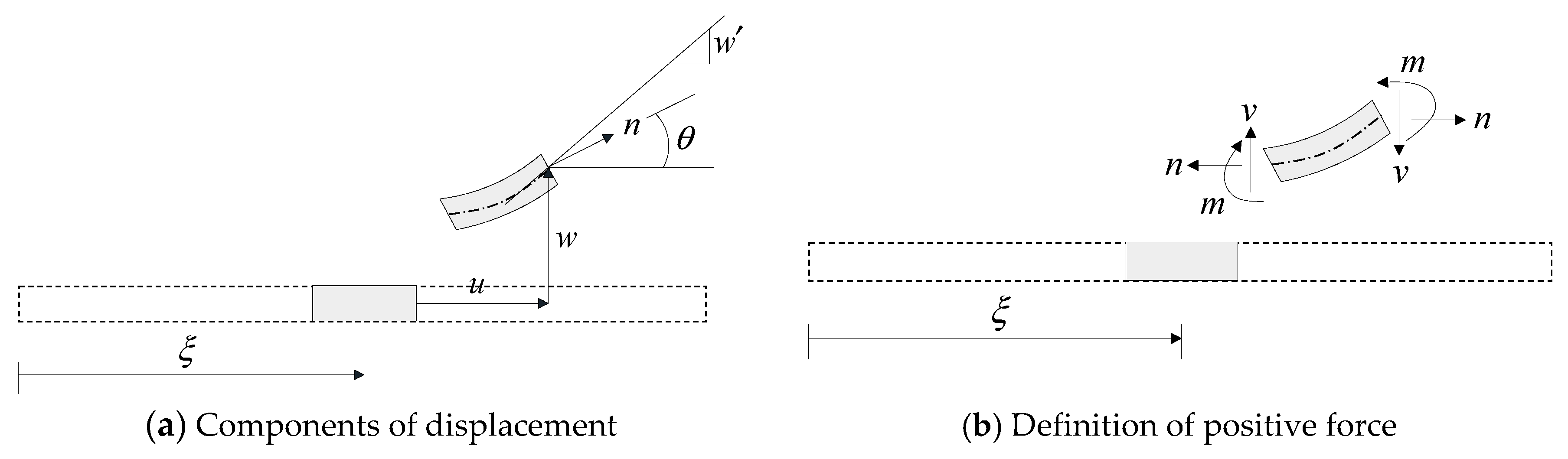the Bernoulli-Euler beam [14,15]. This simplification yields the stiffer behavior of a short beam, as it neglects shear deformation, which imposes additional rotation of the cross section. The Timoshenko beam suggests a solution to this problem. The equilibrium and strain-displacement equations of the Timoshenko beam can be derived as follows [16],

$$n^{\prime }=p$$

(1a)

$$\epsilon =u^{\prime }$$

(1b)

$$m^{″}=q$$

(1c)

$$\kappa =\theta$$

(1d)

$$v^{\prime }=-q$$

(1e)

$$\gamma =w^{\prime }-\theta$$

(1f)

where, n = axial force field; m = bending moment field; q and p = applied transverse and axial load per unit length, respectively; v = shear force field; $\kappa$ = curvature field; $\gamma$ = shear strain field; $\epsilon$ = axial strain field; w = transverse displacement field; $\theta$ = rotation field; and u = axial displacement field. A prime denotes differentiation with respect to $\xi$, which locates a position in the reference coordinate system, as depicted in Figure 1.

The Timoshenko beam can accurately describe the shear behavior of homogeneous and linear beams. The sectional displacements, including axial and transverse displacements and rotation, can define the normal deformations of each point or layer of the cross section. However, as the required constitutive model to calculate the corresponding stresses is uniaxial, ad-hoc functions, such as shear functions, are required to define shear profiles over the cross section, mostly with parabolic shapes or constant ones. Moreover, the beam shear is uncoupled from the flexural responses, and the description of nonlinear shear evolution of the composite beams that are composed of nonlinear materials is hardly achievable. To resolve this problem, this study suggests a new element formulation to determine shear stress distributions over the cross section.

3. Shear Formulations for Beam Section

The longitudinal stiffness method [7] determines the shear stress distributions based upon equilibrium. Therefore, the method is rigorous in solving nonlinear beams, such as RC beams. The longitudinal stiffness method is rewritten in the context of the finite element method, where more consistent element formulations can be derived.

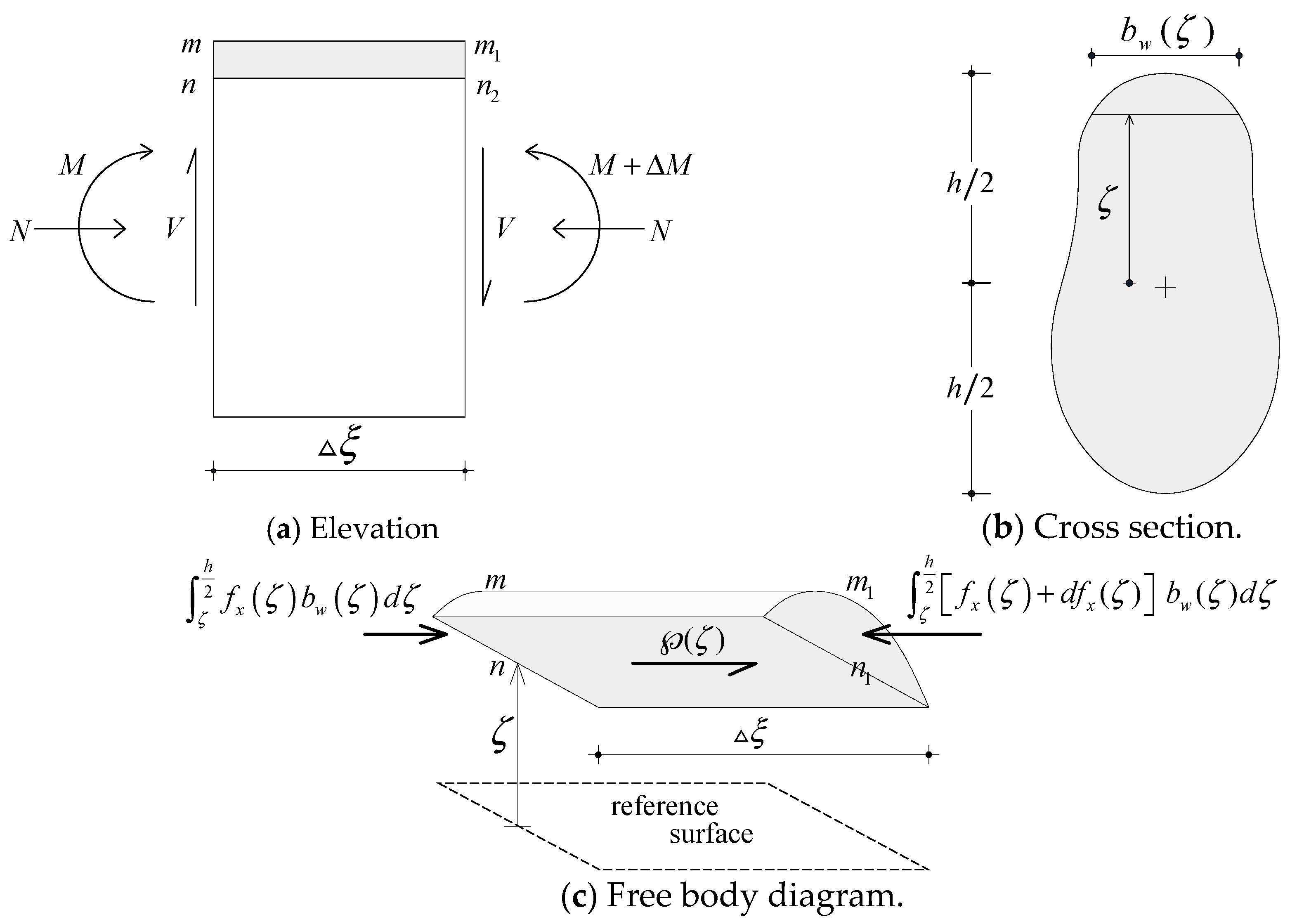
The shear stresses acting on the surface of a layer of the cross section should be equal to the horizontal surface shear stresses acting between layers of the beam from equilibrium. This is the basis by which the shear flow is used to calculate the shear stress distributions. To demonstrate this, let us consider a free body diagram (distributed load omitted), as shown in Figure 2. The shear flow—the horizontal shear force per unit distance along the longitudinal axis of the beam—can be evaluated from equilibrium as:

$$\wp \left(\zeta \right)={\displaystyle {\int }_{\zeta }^{\frac{h}{2}}d{f}_x\left(\zeta \right)}{b}_w\left(\zeta \right)d\zeta$$

(2)

where, $-\frac{h}{2}\le \zeta <\frac{h}{2}$; $d{f}_x\left(\zeta \right)$ denotes the difference of longitudinal stresses between cross-sections mn and m₁n₁, $b_w\left(\zeta \right)$ is the width of the layer at the depth of $\zeta$, and h is the overall height of the section. The horizontal shear stress at $\zeta$ is obtained by dividing the shear flow by the width of the layer at $\zeta$; i.e.,

$$v_{xy}\left(\zeta \right)=\frac{\wp \left(\zeta \right)}{b_w\left(\zeta \right)}$$

(3)

The normal stress gradient or the stress differences between the two sections $d{f}_x$ can be defined as:

$$d{f}_x\left(\zeta \right)=\left[10\right]\mathbf{d}d\epsilon$$

(4)

where, the first term [10] is multiplied to obtain only the scalar normal stress, $\mathbf{d}$ is the 2 × 2 sectional stiffness matrix of the cross section, which will be defined later, and $d\epsilon$ is the 2 × 1 sectional strain vector. The last term is the sectional strain changes due to the moment change $\Delta M$ as shown in Figure 2a, and related to the 3 × 1 full strains as,

$$d\epsilon =\varsigma d\mathbf{e}$$

(5)

And

$$\varsigma \equiv \left[\begin{array}{ccc}1& -\zeta & 0\\ 0& 0& \psi \left(\zeta \right)\end{array}\right]$$

(6)

where, $\psi$ is the shear strain function. Depending on how this is defined results in a constant, parabolic, or other shear distribution. For example, if $\psi \left({\zeta }_k\right)=1$, a constant shear distribution is obtained.

Knowing that Equation (5) defines the sectional strain changes due to the moment change $\Delta M=V$ leads to:

$$d\mathbf{e}={\left[K\right]}^{-1}\left[\begin{array}{l}0\\ V\\ 0\end{array}\right]$$

(7)

Herein, ${\mathbf{K}}_s$ is the full stiffness matrix of the cross section, a.k.a. the longitudinal stiffness matrix. The discretization of Equation (3) and writing the shear stress at the k-th fiber leads to:

$${\nu }_{xy}\left({\zeta }_k\right)=\wp \left({\zeta }_k\right)/b_w\left({\zeta }_k\right)$$

(8)

where, $\wp \left({\zeta }_k\right)={\displaystyle \sum _{j=1}^k{h}_f\left({\zeta }_j\right)}\cdot d{f}_x\left({\zeta }_j\right)\cdot b_w\left({\zeta }_j\right)$, and $h_f\left({\zeta }_j\right)$ is the height of the j-th fiber. Finally, the shear stress function at the k-th fiber is obtained from:

$$\overline{\omega }{\left({\zeta }_k\right)}^{\nu }={\nu }_{xy}\left({\zeta }_k\right)/V_{mi}$$

(9)

It should be noted that the shear distributions are determined from the sectional equilibrium. For equilibrium-driven equations, it is extremely difficult to derive a consistent element formulation in the conventional finite element method, which is based on the displacement-based formulation. Therefore, the authors seek the answer from the force-based formulation that strictly satisfies equilibrium.

4. Two-Dimensional Realization of Beam Shear

As shear is at least two-dimensional, two-dimensional representation of shear is indispensable to obtain more realistic shear distributions. The micro-plane concept is the simplest and widely accepted method among beam shear models because it can be realized in a one-dimensional beam-column element. The micro-plane describes bi-axial states, where two correlated uniaxial states are defined in their principal directions. For an RC beam, the bi-axial states can be defined as follows.

4.1. Concrete Material

There are many constitutive models to simulate the concrete behavior [17,18,19], and those models are widely used in the finite element analysis. In all analyses presented in this paper, the uniaxial behavior of concrete in compression is obtained by applying the modified Kent and Park model [20] to account for the confining effects provided by stirrups. That uniaxial behavior is scaled by using the compression softening relation suggested by Vecchio and Collins [21]. In addition, other concrete models with confinement effect [16,17,18] can be interchangeably used. To describe tension stiffening, the shear cracking stress of concrete is calculated by using the ACI expression $0.17\sqrt{f_c^{\prime }}$, where $f_c^{\prime }$ is in MPa [22]. The post-cracking envelope is obtained by using the equation proposed by Collins and Mitchell [22]. Figure 3 illustrates the uniaxial behavior of concrete material. It is assumed that this uniaxial behavior discussed thus far describes the orthotropic concrete material in the principal directions. The composition of material tangent stiffness for an orthotropic material is discussed as follows.

For an orthotropic material such as concrete, by neglecting the Poisson’s ratio, the material tangent in the principal directions can be written as:

$${\mathbf{d}}_{\mathrm{p}}=\left[\begin{array}{ccc}{E}_1& 0& 0\\ 0& E_2& 0\\ 0& 0& G\end{array}\right]$$

(10)

where, $E_1$ and $E_2$ are the Young’s modulus in each principal direction, respectively, which can be calculated by using the ACI expression $4700\sqrt{f_c^{\prime }}$, and $G$ is the shear modulus. The latter can be determined by:

$$G=\frac{f_1-f_2}{2\left({\epsilon }_1-{\epsilon }_2\right)}$$

(11)

where, $f_1$ and $f_2$ are the principal stresses, and ${\epsilon }_1$ and ${\epsilon }_2$ are the principal strains. Equation (11) satisfies the condition of invariance under the principal axis rotation [23]. The orthotropic material stiffness should be transformed to the current local coordinate system of the element by using the following relation:

$$\widehat{\mathbf{d}}={\mathbf{T}}^{\mathrm{T}}\cdot {\mathbf{d}}_{\mathrm{p}}\cdot \mathbf{T}$$

(12)

where the transformation matrix is defined as:

$$\mathbf{T}=\left[\begin{array}{ccc}{\cos }^2\theta & {\sin }^2\theta & \cos \theta \sin \theta \\ {\sin }^2\theta & {\cos }^2\theta & -\cos \theta \sin \theta \\ -2\cos \theta \sin \theta & 2\cos \theta \sin \theta & {\cos }^2\theta -{\sin }^2\theta \end{array}\right]$$

(13)

The failure criterion of concrete material can be found in the modified compression field theory (MCFT) formulation [7], where the two-dimensional plane reinforced concrete response was simplified with two uni-axial stress-strain relations in the two principal directions. In the principal directions, the compression failure occurs at the compression strain of −0.003. The steel was considered as smeared to the corresponding concrete layers, and the confining effects were also reflected, as described in Figure 3.

4.2. Steel Material

A bi-linear behavior with a certain strain hardening ratio is assumed for steel. The material tangent for steel can be written as:

$$\widehat{\mathbf{d}}=\left[\begin{array}{ccc}{E}_x& 0& 0\\ 0& E_y& 0\\ 0& 0& 0\end{array}\right]$$

(14)

where, the subscripts x and y represent the longitudinal and vertical directions, respectively. The former is the axis of the longitudinal bars, and the latter is that of the stirrups.

In a beam-column element, the aforementioned two-dimensional states should be driven from the uniaxial strain of each layer of the cross section. This involves the matrix condensation with the assumption of zero traction in the vertical direction and the shear stress function that was presented before.

5. Force-Based Element Formulation of the Timoshenko Beam

For the realization of the aforementioned shear functions and two-dimensional beam shear, first, the element formulation is derived followed by the presentation of the solution strategy. The force-based element formulation of the Timoshenko beam is derived by directly integrating the governing equations.

5.1. Direct Integration of the Equations of Equilibrium

Define the following functions as integrals of the applied transverse and axial loads [16]:

$$Q\left(\xi \right)\equiv {\displaystyle {\int }_0^{\xi }q\left(\eta \right)}d\eta$$

(15a)

$$M\left(\xi \right)\equiv {\displaystyle {\int }_0^{\xi }\eta q\left(\eta \right)}d\eta$$

(15b)

$$P\left(\xi \right)\equiv {\displaystyle {\int }_0^{\xi }p\left(\eta \right)}d\eta$$

(15c)

The integration of Equation (1c) gives:

$$m^{\prime }\left(\xi \right)=Q\left(\xi \right)+c_1=\left(1-\frac{\xi }{L}\right)Q\left(\xi \right)+\frac{\xi }{L}Q\left(\xi \right)+c_1$$

(16)

Applying the integration by parts, and integrating the equation above, leads to:

$$\begin{array}{ll}m\left(\xi \right)& =\left(\xi -\frac{{\xi }^2}{2L}\right)Q\left(\xi \right)-{\displaystyle {\int }_0^{\xi }\left(\eta -\frac{{\eta }^2}{2L}\right)}q\left(\eta \right)d\eta +\frac{{\xi }^2}{2L}Q\left(\xi \right)-{\displaystyle {\int }_0^{\xi }\frac{{\eta }^2}{2L}}q\left(\eta \right)d\eta +c_1\xi +c_2\\ & =\xi Q\left(\xi \right)-{\displaystyle {\int }_0^{\xi }\eta }q\left(\eta \right)d\eta +c_1\xi +c_2\\ & =\xi Q\left(\xi \right)-M\left(\xi \right)+c_1\xi +c_2\end{array}$$

(17)

By solving for the constants and rearranging the equation above, we obtain:

$$m\left(\xi \right)=m_0{b}_1\left(\xi \right)+m_L{b}_2\left(\xi \right)+\frac{\xi }{L}\overline{M}-M\left(\xi \right)+\left[Q\left(\xi \right)-\overline{Q}\right]\xi$$

(18)

where, $b_1\left(\xi \right)\equiv 1-\xi /L$; $b_2\left(\xi \right)\equiv \xi /L$; $m_0\equiv m\left(0\right)$; $m_L\equiv m\left(L\right)$; $\overline{M}\equiv M\left(L\right)$; and $\overline{Q}\equiv Q\left(L\right)$. The integration of Equation (1e) and rearrangement give:

$$\nu \left(\xi \right)=-Q\left(\xi \right)+{\nu }_0$$

(19)

where, ${\nu }_0=\nu \left(0\right)$. From Equation (19) and knowing that $m^{\prime }=-\nu$, we can obtain:

$$\begin{array}{ll}m\left(\xi \right)& ={\displaystyle {\int }_0^{\xi }Q}\left(\eta \right)d\eta -{\nu }_0\xi +m_0\\ & =\xi Q\left(\xi \right)-{\displaystyle {\int }_0^{\xi }\eta q}\left(\eta \right)d\eta -{\nu }_0\xi +m_0\end{array}$$

(20)

Along with Equation (15), substituting L into Equation (20) and solving for v₀ give:

$${\nu }_0=-\frac{m_L}{L}+\overline{Q}-\frac{\overline{M}}{L}+\frac{m_0}{L}$$

(21)

Rearranging Equation (19) leads to:

$$\nu \left(\xi \right)=-Q\left(\xi \right)-\frac{m_L}{L}+\overline{Q}-\frac{\overline{M}}{L}+\frac{m_0}{L}$$

(22)

The integration of Equation (1a) and rearrangement give:

$$n\left(\xi \right)=n_0+P\left(\xi \right)$$

(23)

where, $n_0=n\left(0\right)$.

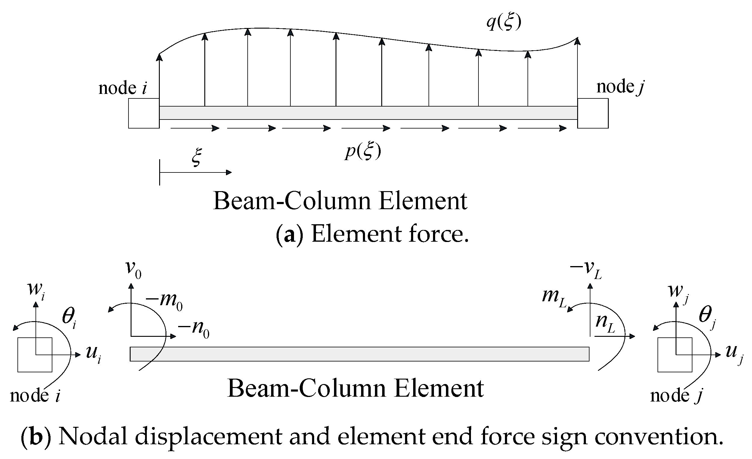
Let us denote the force field and the discrete element force parameters as:

$$\mathsf{\sigma }\left(\xi \right)\equiv {\left[n\left(\xi \right),m\left(\xi \right),\nu \left(\xi \right)\right]}^T$$

(24)

$$\mathbf{s}\equiv {\left[n_0,m_0,m_L\right]}^T$$

(25)

The force field can be written as:

$$\mathsf{\sigma }\left(\xi \right)={\mathbf{b}}^T\left(\xi \right)\mathbf{s}+{\mathsf{\sigma }}^p\left(\xi \right)$$

(26)

where, ${\mathbf{b}}^T\left(\xi \right)$ and the particular force field ${\mathsf{\sigma }}^p\left(\xi \right)$ are defined as:

$${\mathbf{b}}^T\left(\xi \right)\equiv \left[\begin{array}{ccc}1& 0& 0\\ 0& b_1\left(\xi \right)& b_2\left(\xi \right)\\ 0& 1/L& -1/L\end{array}\right]$$

(27)

$${\mathsf{\sigma }}^p\left(\xi \right)\equiv \left[\begin{array}{c}P\left(\xi \right)\\ \frac{\xi }{L}\overline{M}-M\left(\xi \right)+\left[Q\left(\xi \right)-\overline{Q}\right]\xi \\ -\frac{\overline{M}}{L}+\overline{Q}-Q\left(\xi \right)\end{array}\right]$$

(28)

The end forces can be defined as:

$$\widehat{\mathbf{s}}\equiv {\left[-n_0,{\nu }_0,-m_0,n_L,-{\nu }_L,m_L\right]}^T$$

(29)

as shown in Figure 4.

This can be expressed in terms of the essential force parameters and the applied loads as [16]:

$$\widehat{\mathbf{s}}=\mathbf{Ls}+\mathbf{P}$$

(30)

where, the equivalent nodal load vector is denoted:

$$\mathbf{P}=\left[\begin{array}{cccccc}0& \overline{M}/L-Q& 0& \overline{P}& -\overline{M}/L& 0\end{array}\right]$$

(31)

and the matrix L is given by:

$${\mathbf{L}}^T=\left[\begin{array}{cccccc}-1& 0& 0& 1& 0& 0\\ 0& 1/L& -1& 0& -1/L& 0\\ 1& 1/L& 0& 1& -1/L& 1\end{array}\right]$$

(32)

5.2. Direct Integration of the Differential Strain-Displacement Equations

Integrating the strain-displacement equations of Equations (1b), (1d), and (1f) gives:

$$\frac{w_L-w_0}{L}-\frac{1}{L}{\displaystyle {\int }_0^L\gamma \left(\xi \right)}d\xi -{\displaystyle {\int }_0^L{b}_1\left(\xi \right)\kappa }d\xi =0$$

(33a)

$${\theta }_L-{\theta }_0-\frac{w_L-w_0}{L}+\frac{1}{L}{\displaystyle {\int }_0^L\gamma (\xi )d\xi -{\displaystyle {\int }_0^L\frac{\xi }{L}\kappa (\xi )d\xi =0}}$$

(33b)

$$-u_0+u_L-{\displaystyle {\int }_0^L\epsilon (\xi )d\xi =0}$$

(33c)

This can be written in matrix form as:

$${\mathbf{L}}^T\mathbf{w}-{\displaystyle {\int }_0^L\mathbf{b}(\xi )\mathbf{e}(\xi )}d\xi =0$$

(34)

where,$\mathbf{w}\equiv {\left[u_0,w_0,{\theta }_0,u_L,w_L,{\theta }_L\right]}^T$; $\mathbf{e}\equiv {\left[\epsilon \left(\xi \right),\kappa \left(\xi \right),\gamma \left(\xi \right)\right]}^T$. The detailed derivation of the above equations can be found in reference [24], and it was developed by adopting the direct integration [25].

6. State Determination

In the direct stiffness method, the equations of motion, which are constructed by assembling the element state quantities, can be solved by using any Newton-type iteration method. This reduces the difference between the internal force and external force through iterations. This also holds for the nonlinear flexibility-based method, as the element stiffness matrix is obtained by inverting the element flexibility matrix. The latter is obtained from the integration of the quadratic product of the section flexibility and force interpolation function matrix. However, in contrast to the stiffness-based method, the flexibility-based method requires an additional iteration loop to satisfy compatibility conditions. This is discussed in the following.

6.1. Fiber State Determination

The section strain is discretized to obtain the strain at the k-th fiber by using the following equation:

$${\mathsf{\epsilon }}_{mik}\equiv {\mathsf{\varsigma }}_{mik}{\mathbf{e}}_{mi}$$

(35)

where, ${\mathsf{\epsilon }}_{mik}\equiv {\mathsf{\epsilon }}_m\left({\xi }_{ik}\right)$; ${\xi }_{ik}\equiv {\xi }_i\left({\zeta }_k\right)$; ${\xi }_{ik}$ is the vertical coordinate, as shown in Figure 5; $\mathsf{\epsilon }\equiv {\left[{\epsilon }_x\left(\zeta \right),{\gamma }_{xy}\left(\zeta \right)\right]}^T$, where ${\epsilon }_x\left(\zeta \right)$ and ${\gamma }_{xy}\left(\zeta \right)$ are the normal and shear strains, respectively; ${\mathsf{\varsigma }}_{mik}$ is the base function as defined earlier. The fiber stress $\mathsf{\phi }$ is then obtained from:

$$\mathsf{\phi }\equiv \tilde{\mathsf{\phi }}\left(\mathsf{\epsilon }\right)$$

(36)

where, $\mathsf{\phi }\equiv {\left[f_x\left(\zeta \right),{\nu }_{xy}\left(\zeta \right)\right]}^T$; $f_x\left(\zeta \right)$ and ${\nu }_{xy}\left(\zeta \right)$ are the normal and shear stresses, respectively.

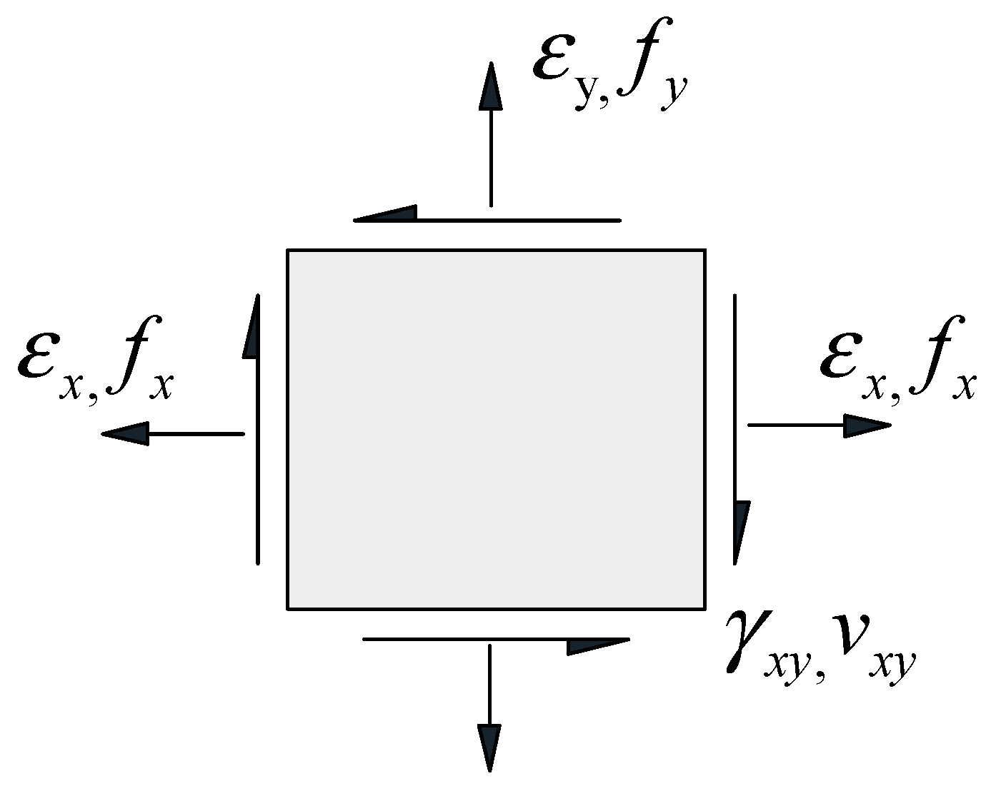
If a biaxial constitutive law is used for the material, additional strain and stress fields should be considered; those are ${\epsilon }_y$ and $f_y$ for strain and stress, respectively. The complete biaxial state of an infinitesimal element is depicted in Figure 6, and the stress-strain relations are given in Equation (30) in the incremental form after linearization.

$$\Delta {\widehat{\mathsf{\phi }}}^v={\widehat{\mathbf{d}}}_{mik}^{v-1}\Delta {\widehat{\mathsf{\epsilon }}}^v$$

(37)

where, $\widehat{\mathsf{\phi }}\equiv \left[f_x,f_y,{\nu }_{xy}\right]$; $\widehat{\mathsf{\epsilon }}\equiv \left[{\epsilon }_x,{\epsilon }_y,{\gamma }_{xy}\right]$. A general approach to retrieve the additional quantities assumes $f_y=0$ at any location of a beam. Therefore, through static condensation, the biaxial state can be reduced to:

$$\Delta {\mathsf{\phi }}^v={\mathbf{d}}_{mik}^{v-1}\Delta {\mathsf{\epsilon }}^v$$

(38)

where, ${\mathbf{d}}_{mik}=\left[\begin{array}{cc}{\widehat{\mathrm{d}}}_{11}& {\widehat{\mathrm{d}}}_{13}\\ {\widehat{\mathrm{d}}}_{31}& {\widehat{\mathrm{d}}}_{33}\end{array}\right]-\left[\begin{array}{c}{\widehat{\mathrm{d}}}_{12}\\ {\widehat{\mathrm{d}}}_{32}\end{array}\right]{\left[{\widehat{\mathrm{d}}}_{22}\right]}^{-1}\left[\begin{array}{cc}{\widehat{\mathrm{d}}}_{21}& {\widehat{\mathrm{d}}}_{23}\end{array}\right]$.

6.2. Solution Strategy

The flexibility-based method works together with force interpolation functions, for which reason it is also known as the force-based method. This method allows the solution of the system of equations without shape functions. A similar principle is taken in the determination of the fiber state, where shear stress functions (or shear interpolation functions) are known. The predictor and corrector phases, which determine the section shear force $V_{mi}$ for the known section strain ${\mathbf{e}}_{mi}$, will be explained in the following.

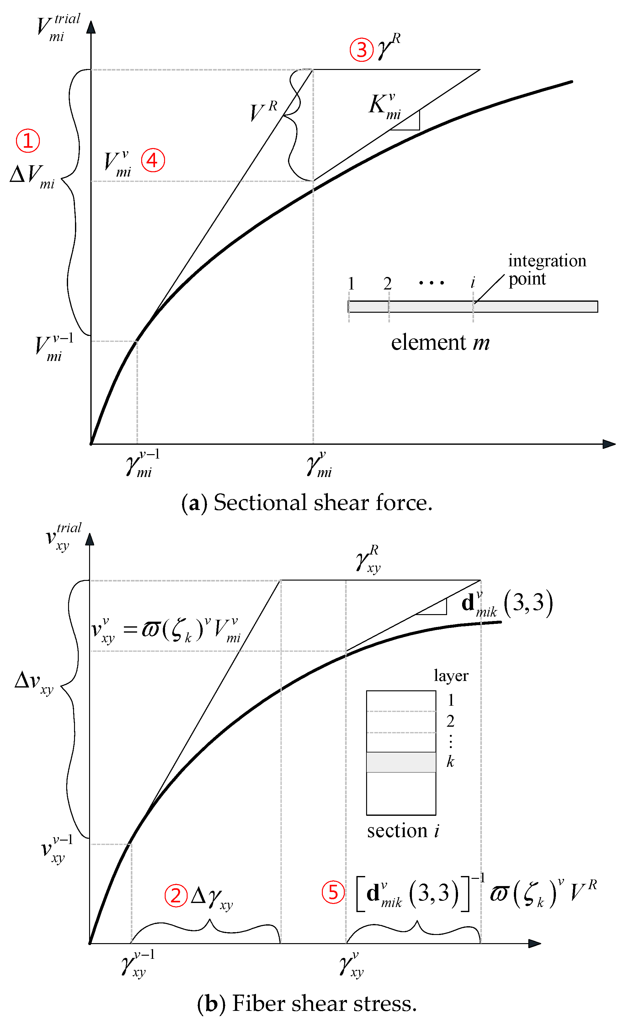
6.2.1. Predictor Phase

Step 1: The trial section shear force is determined from the following relation:

$$V_{mi}^{trial}\equiv \Delta V_{mi}+V_{mi}^{v-1}$$

(39)

where, $\Delta V_{mi}=\left[\begin{array}{ccc}0& 0& 1\end{array}\right]K_{mi}^{\nu -1}\Delta {\mathbf{e}}_{mi}$.

Step 2: The axial strain is evaluated by using the plane-section assumption but the vertical and shear strains are calculated through matrix condensation; i.e., in an incremental form:

$$\Delta {\epsilon }_y=-{\left[{\widehat{\mathbf{d}}}_{mik}^{v-1}(2,2)\right]}^{-1}\cdot \left({\widehat{\mathbf{d}}}_{mik}^{v-1}(2,1)\cdot \Delta {\epsilon }_x+{\widehat{\mathbf{d}}}_{mik}^{v-1}(2,3)\cdot \Delta {\nu }_{xy}\right)$$

(40)

$$\Delta {\gamma }_{xy}={\left[{\mathbf{d}}_{mik}^{v-1}(2,2)\right]}^{-1}\cdot \left(\Delta {\nu }_{xy}-{\mathbf{d}}_{mik}^{v-1}(2,2)\cdot \Delta {\epsilon }_x\right)$$

(41)

where, $\Delta {\nu }_{xy}={\nu }_{xy}^{trial}-{\nu }_{xy}^{v-1}$. Since all the strain values are known, the corresponding stresses can be evaluated by using any biaxial constitutive model. Then, the corrector phase follows, because the shear stress obtained from a constitutive relation will differ from the trial shear stress.

6.2.2. Corrector Phase

Step 3: In the corrector phase, the shear strain is corrected in a way that reduces the shear stress residuals. However, in the flexibility method, strain residuals instead of stress are integrated to give the counterpart in the upper level. Therefore, the section shear strain residual is obtained as:

$${\gamma }^R\left({\xi }_{mi}\right)\equiv {\displaystyle \sum _{k=1}^q{h}_f\left({\zeta }_k\right)\cdot \overline{\omega }\left({\zeta }_k\right)\cdot {\gamma }_{xy}^R}$$

(42)

where, ${\gamma }_{xy}^R\equiv {\left[{\mathbf{d}}_{mik}^v(3,3)\right]}^{-1}{\nu }_{xy}^R$, and $\overline{\omega }$ is the shear stress functions discussed later. The superscript R denotes residual.

Step 4: The section shear force is now corrected by the following relation; i.e.,

$$V_{mi}^v=V_{mi}^{trial}-V^R$$

(43)

where, $V^R\equiv {\mathbf{K}}_{mi}^v{\gamma }^R\left({\xi }_{mi}\right)$.

Step 5: The fiber state should also be corrected as given below:

$${\mathsf{\epsilon }}_{mik}^v={\mathsf{\epsilon }}_{mik}^{v-1}+\Delta \mathsf{\epsilon }+{\gamma }_{xy}^R\mathbf{1}-{\left[{\mathbf{d}}_{mik}^v(3,3)\right]}^{-1}\overline{\omega }{\left({\zeta }_k\right)}^v{V}^R$$

(44)

$${\mathsf{\phi }}_{mik}^v=\mathsf{\iota }{\tilde{\mathsf{\phi }}}_{mik}^v+\overline{\omega }{\left({\zeta }_k\right)}^v{V}_{mi}^v\mathbf{1}$$

(45)

where, $\mathbf{1}\equiv [\begin{array}{ccc}0& 0& 1\end{array}]$; $\mathsf{\iota }\equiv diag\left(\left[\begin{array}{ccc}1& 1& 0\end{array}\right]\right)$; ${\tilde{\mathsf{\phi }}}_{mik}^v\equiv \tilde{\mathsf{\phi }}({\mathsf{\epsilon }}_{mik}^v)$ is the fiber resisting stress obtained from a constitutive relation for a known ${\mathsf{\epsilon }}_{mik}^v$. Note that each step is indicated with a circular number at the corresponding location in Figure 7 for the illustration purpose.

6.2.3. Update of Section Stiffness and Resisting Force

The section stiffness is updated by using Equation (26) with the following updated base function:

$${\mathsf{\varsigma }}_{mik}^v\equiv \left[\begin{array}{ccc}1& -{\zeta }_k& 0\\ 0& 0& \psi ({\zeta }_k)\end{array}\right]$$

(46)

where, $\psi ({\zeta }_k)\equiv {\gamma }_{xy}({\zeta }_k)/{\vartheta }_k$; ${\vartheta }_k\equiv {\displaystyle \sum _{k=1}^q[h_f({\zeta }_k)b_w({\zeta }_k)v_{xy}^{trial}({\zeta }_k){\gamma }_{xy}({\zeta }_k)]}/V_{mi}^{trial}$.

The numerator of the latter is the work done by the internal shear stress. Therefore, it satisfies the principle of virtual work. Finally, the resisting force vector has the expression:

$${\mathsf{\sigma }}_{mi}^v={\displaystyle \sum _{k=1}^q\left[h_f({\zeta }_k)b_w({\zeta }_k){\left[{\mathsf{\varsigma }}_{mik}^v\right]}^T{\tilde{\mathsf{\phi }}}_{mik}^v\right]}$$

(47)

7. Constitutive Relation

For the v-th iteration, the internal force vector for section i of element m can be obtained from the relation [25]:

$$\mathsf{\sigma }=\widehat{\mathsf{\sigma }}\left({\mathbf{e}}_{mi}^v\right)$$

(48)

where, ${\mathbf{e}}_{mi}^v={\mathbf{C}}_{mi}^{v-1}\Delta {\mathsf{\sigma }}_{mi}^{v-1}+{\mathbf{e}}_{mi}^{v-1}$; ${\mathbf{e}}_{mi}\equiv {\mathbf{e}}_m\left({\xi }_i\right)$; ${\mathbf{C}}_{mi}^{v-1}\equiv {\left[{\mathbf{D}}_{mi}^{v-1}\right]}^{-1}$ is the section tangent compliance from the previous step; and $\Delta$ denotes an increment operator. The tangent stiffness at the known strain $\mathbf{e}$ is evaluated for element m as:

$${\mathbf{D}}_{mi}^v\equiv {\left[\frac{\partial \widehat{\mathsf{\sigma }}\mathbf{(}\mathbf{e}\mathbf{)}}{\partial \mathbf{e}}\right]}_{\mathbf{e}={\mathbf{e}}_{mi}^v}={\left[{\mathbf{C}}_{mi}^v\right]}^{-1}$$

(49)

Through numerical integration, the element flexibility matrix has the expression:

$${\mathbf{F}}_m^v\equiv {\displaystyle \sum _{i=1}^p{\omega }_i{\mathbf{b}}_{mi}{\mathbf{C}}_{mi}^v{\mathbf{b}}_{mi}^T}$$

(50)

where, ${\omega }_i$ is the weights. Inverting this gives the element stiffness matrix; i.e., ${\left[{\mathbf{K}}_m^v\right]}^{-1}={\mathbf{F}}_m^v$. The section tangent stiffness can be calculated from the fiber model. The section tangent stiffness can be obtained by:

$${\mathbf{D}}_{mi}^v={\displaystyle \sum _{k=1}^q{A}_k{\mathsf{\varsigma }}_{mik}^T{\mathbf{d}}_{mik}{\mathsf{\varsigma }}_{mik}}$$

(51)

where, $A_k$ is the area of the k-th fiber on the cross-section, and ${\mathbf{d}}_{mik}\equiv \partial {\mathsf{\phi }}_{mik}(\mathsf{\epsilon })/\partial \mathsf{\epsilon }$ is the material tangent as defined earlier.

8. Model Evaluation

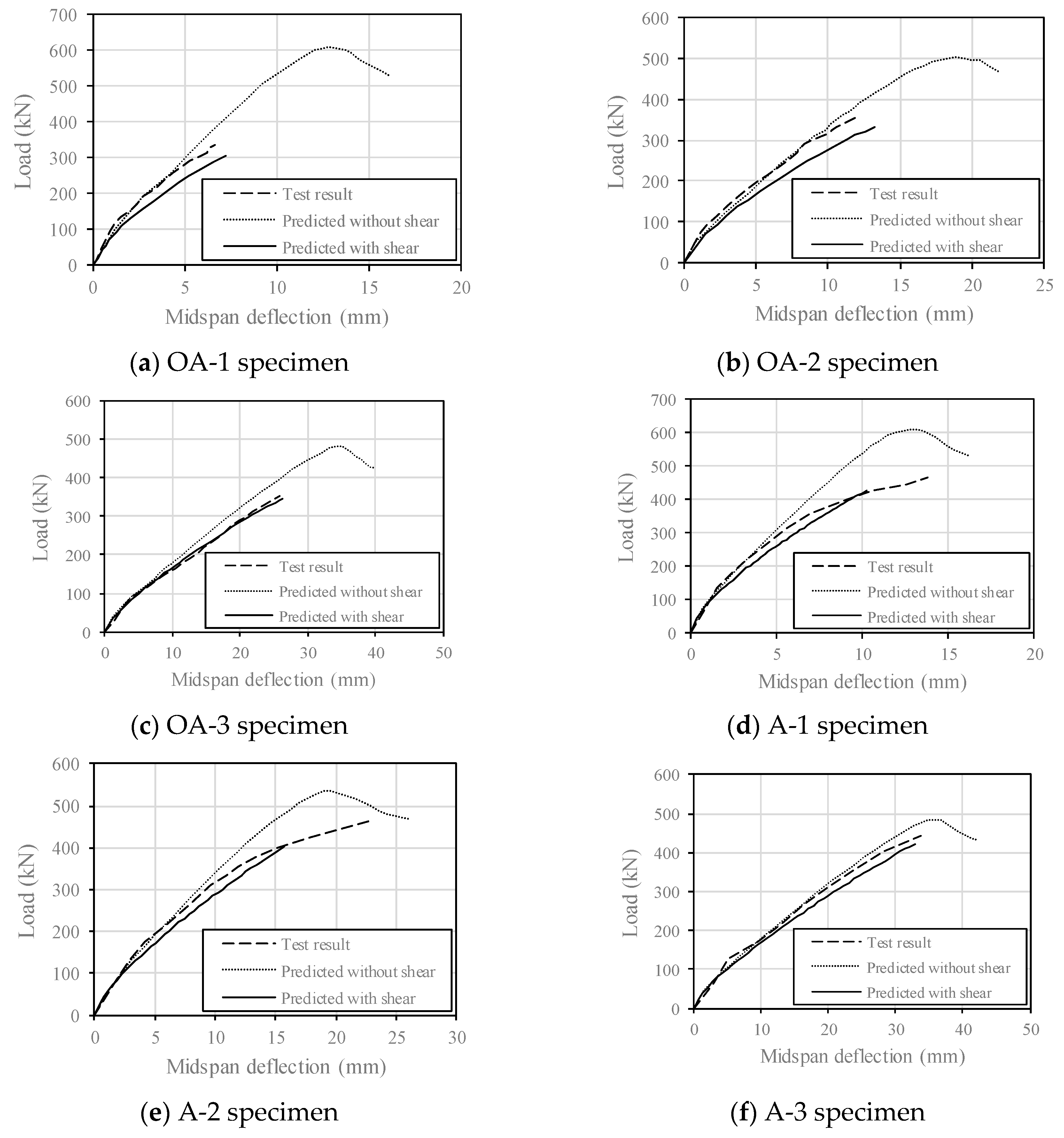
The proposed model was evaluated on the RC beam test data reported by Bresler and Scordelis [26]. In this test, they obtained various failure modes, such as diagonal tension, shear-compression, and flexure-compression failures, by changing the shear span ratios. Another key variable was the existence of web reinforcement. Among those test specimens, the specimens OA-1 through OA-3, which did not contain stirrups, and A-1 through A-3, which contained stirrups, were selected in this presentation. The numbers 1, 2, and 3 denote the IDs that indicate the different shear span ratios, 4.0, 5.0, and 7.0, respectively. Figure 8 illustrates the sectional dimensions of the selected members, while

Table 1. Dimensions and material properties of test specimens.

Specimen	f′c (MPa)	Span (m)	a/d	Spacing of Stirrups (mm)	Failure Mode
OA-1	22.5	3.66	3.97	-	Diagonal tension failure
OA-2	23.7	4.57	4.90	-	Diagonal tension failure
OA-3	37.6	6.40	6.94	-	Diagonal tension failure
A-1	24.1	3.66	3.92	210	Shear compression failure
A-2	24.3	4.57	4.93	210	Shear compression failure
A-3	35.0	6.40	6.91	210	Flexure-compression failure

summarizes the test program and the results.

Each member was analyzed by using two different elements: A Bernoulli-Euler beam element with cubic shape functions, and the proposed element. The former, driven from a stiffness-based formulation, was used to illustrate the flexural response of a beam, and the latter to include the shear effects. In the analysis model, only a half of each beam was considered, to take advantage of the symmetry. It was modeled with four elements, each of which had four Gauss-Lobatto integration points.

An arc-length method was used to capture a post-peak response, if any. The numerical response was terminated when numerical problems arose, usually with the satisfaction of the transverse equilibrium equations for all shear elements. For the Bernoulli-Euler beam element, the termination point was selected at a few steps after the post-peak response was obtained.

9. Results

Figure 9 compares the predicted and observed curves of load versus midspan deflection relations. The prediction by using the Bernoulli-Euler beam element is denoted as predicted without shear, and the one by using the proposed element as predicted with shear. In the test results, it can be observed that when no stirrup is present, the strength drops. The strength reduction was significant, especially in the members with a small shear span ratio.

The predictions without shear present the flexural response only; therefore, there was no effect of the stirrups. This explains why the predictions without shear in series OA were similar to the counterparts in series A. As shown in the figure, the predictions without shear showed a higher member strength and stiffness and higher ductility than those with shear. The discrepancy between the two predictions, which represents the shear contribution to the deflection, increased proportionally as the applied load increased. Generally speaking, the curves of the test results corresponded well to those without shear up to the point of half of the ultimate strength but became closer to them with shear afterwards. For most cases, the proposed model predicted the strength of the actual beams satisfactorily, while the model without shear consideration predicted twice as much as the actual shear strength, depending on the problem. For specimen A-1 and 2, the analysis with the proposed model was terminated shortly before it reached the actual strength. However, as can be seen in the figure, the termination points were closely related to the points where the slope of the curve of test changes abruptly.

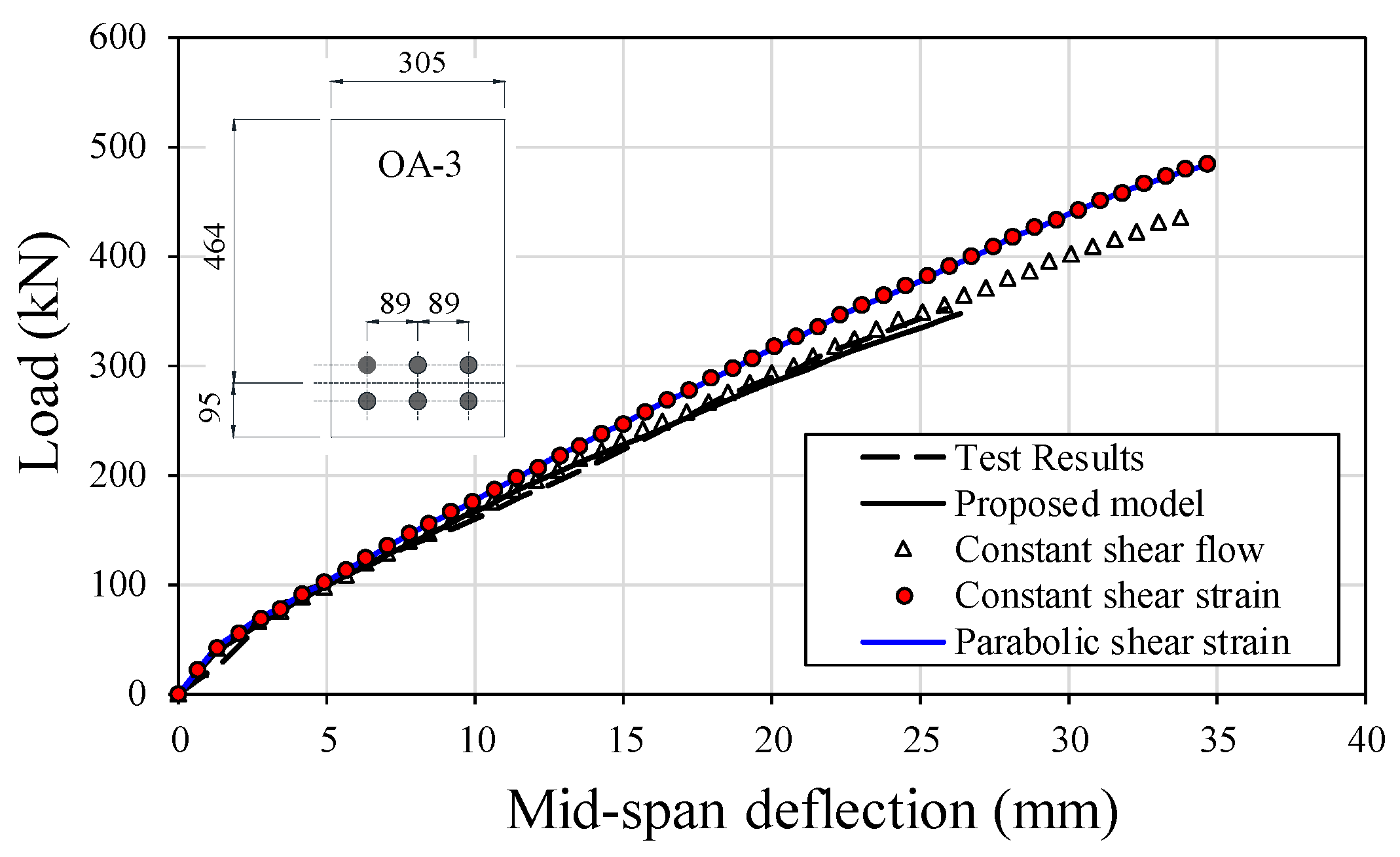
Comparison with Other Shear Models

1. Rectangular beam: The analysis results obtained for specimen OA-3 were compared with those by other shear models, such as (1) constant, or (2) parabolic shear strain model, and (3) constant shear flow model. The constant and parabolic shear strain models assumed the predefined shear strain functions over the cross-section first and then estimated the corresponding shear stresses. The advantage of the shear strain models was that the calculation procedure was simple, but those models can result in redundant constraints. On the other hand, the constant shear flow model, in which the shear force acting on the section considered is given first to obtain the shear strain of the section, can provide a more accurate shear response than the shear strain models.

The constant and parabolic shear strain distributions were obtained by using the following relations for $\psi \left({\zeta }_k\right)$ in Equation (6):

$$\psi \left({\zeta }_k\right)=1$$

(52a)

$$\psi ({\zeta }_k)=\frac{3}{2}\left[1-{\left(\frac{{\zeta }_k}{h/2}\right)}^2\right]$$

(52b)

The constant shear flow model by using the secant stiffness method was discussed by Vecchio and Collins [6]. The shear stresses were determined by dividing a given section shear force by the height of each fiber (or layer). In the proposed model, the constant shear flow model was applied by replacing Equation (2) with the following relation:

$$\wp (\zeta )=\frac{V^{Trial}}{b_w(\zeta )}$$

(53)

Figure 10 shows the comparison of the load-deflection relations obtained by using four different shear models. All four models showed similar initial stiffness up to the first cracking point, where the curves started to diverge. The parabolic and constant shear strain models, which had predefined shear strain distribution shape, showed a very similar response. In comparison with these models, the proposed model and constant shear flow models, which were a force-based method, showed a relatively softer behavior. This discrepancy between the constant/parabolic shear strain methods and the force-based methods comes from the fact that shear strains over the cross-section were assumed as the predefined shapes, such as a constant or parabolic, in the constant/parabolic shear strain methods, while they are not in the force-based method, because the predefined shear strains inevitably create redundant constraints in the deformability of the cross-section. In the force-based method, the shear stresses over the cross-section are calculated from equilibrium, and afterwards, the corresponding shear strains were determined, which does not cause such redundant constraints. The curve obtained by using the proposed model was closely related to the actual behavior with regards to both stiffness and strength. It is clear from the figure that the proposed model predicted the shear strength most accurately, provided that the termination point caused by the vertical equilibrium instability defined the shear failure point.

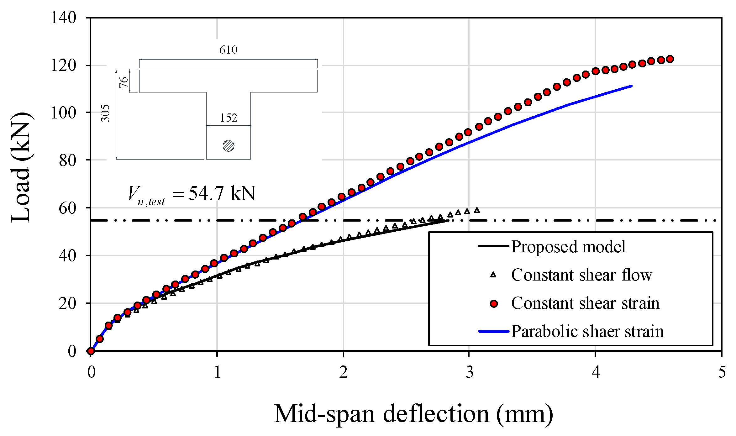
2. T-beam: The advantage that the proposed model possesses is that it describes the shear strain distributions over the cross section very accurately, and, therefore, the state of the section as well. This can best be illustrated by using T-beams, the section of which has larger shear strength than a rectangular section with the same depth and height. For this problem, the predefined shear strain methods, such as constant or parabolic shear strain method, would overestimate the shear strength by drawing more shear stress in the flange area, and keeping the web area stressed in lower intensity.

A T-beam (beam no.: T2) was selected from the extensive test conducted by Placas and Regan [27]. The sectional dimensions are: The web width is 152 mm; the total depth is 305 mm; the depth to the center of the steel is 272 mm; $A_s/b^{\prime }d$ = 1.46%; the flange breadth is 76 mm; and the flange width is 610 mm. The material properties are: The compressive concrete strength is 28.1 MPa, and the yield strength of the longitudinal bar is 620 MPa. The shear span ratio (a/d) is 3.36, and the beam was subjected to a central-point loading. The beam failed at the shear force of 54.7 kN by diagonal tension cracking.

Figure 11 shows the applied shear force versus the mid-span deflection curves obtained by using the four different shear models. The force-based model, including the proposed model and the constant shear flow model, terminated the analysis around the ultimate shear strength of the beam observed in the actual test. In contrast, the predefined shear strain models, including the parabolic shear strain model and the constant shear strain model, led to a shear strength more than twice as much as the actual shear strength; the analysis with the latter continued beyond the end point shown in the figure. The predefined shear strain models gave much stiffer response than the force-based models. For example, at the shear force of 54.7 kN, the constant shear strain model gave the mid-span deflection value of half as much as that obtained by the proposed model.

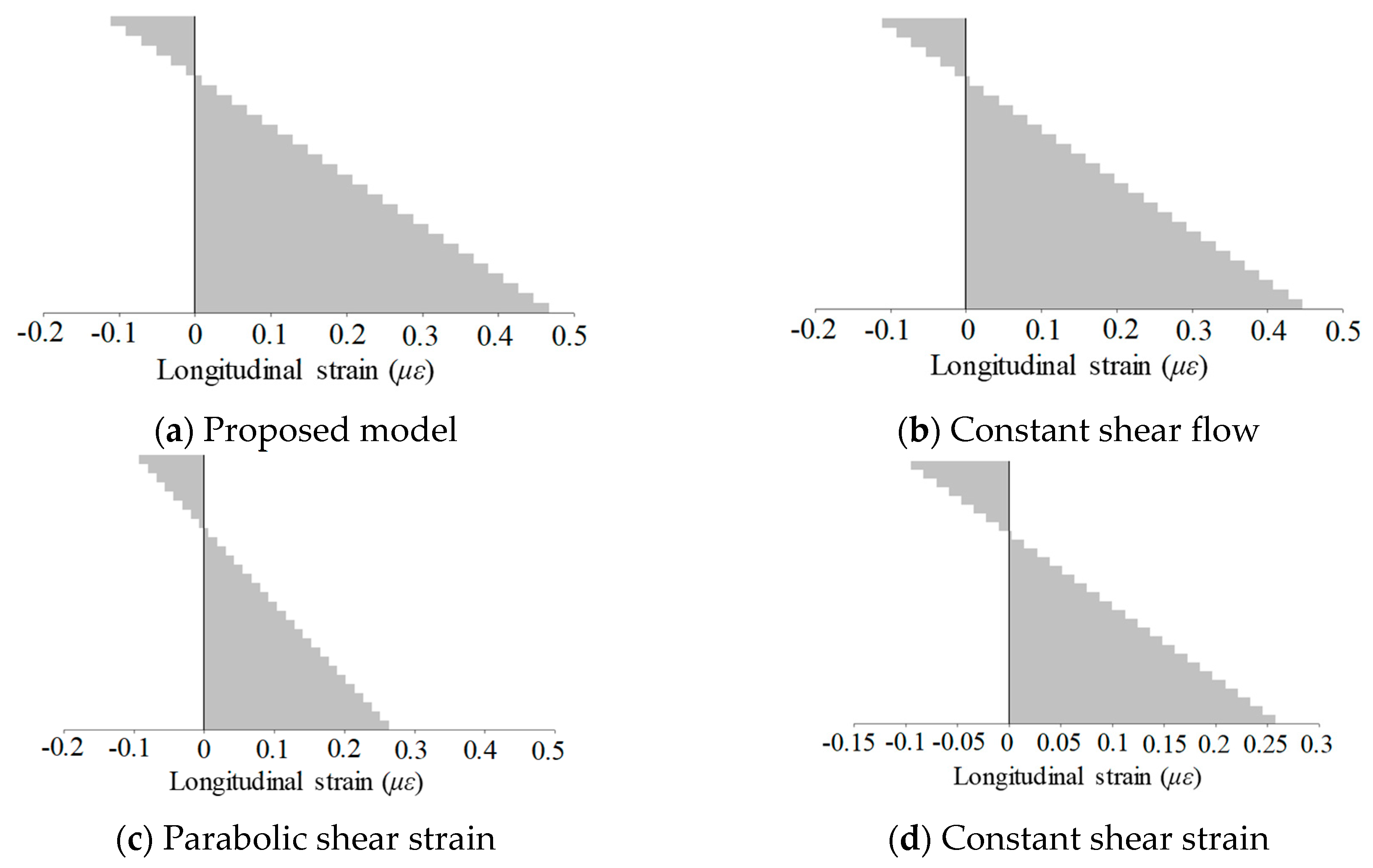
To explain these discrepancies, the local behaviors were compared at the critical section (the effective depth away from the support) at the shear force of 54.7 kN, as shown in Figure 12, Figure 13 and Figure 14. Figure 12 shows that the moment curvature values were analogous to the previous findings. The proposed model showed the largest curvature—more than twice as much as that of the constant shear strain model—and the smallest neutral surface depth. This suggests that the different shear model significantly affects the flexural behavior for the beam having a non-rectangular section.

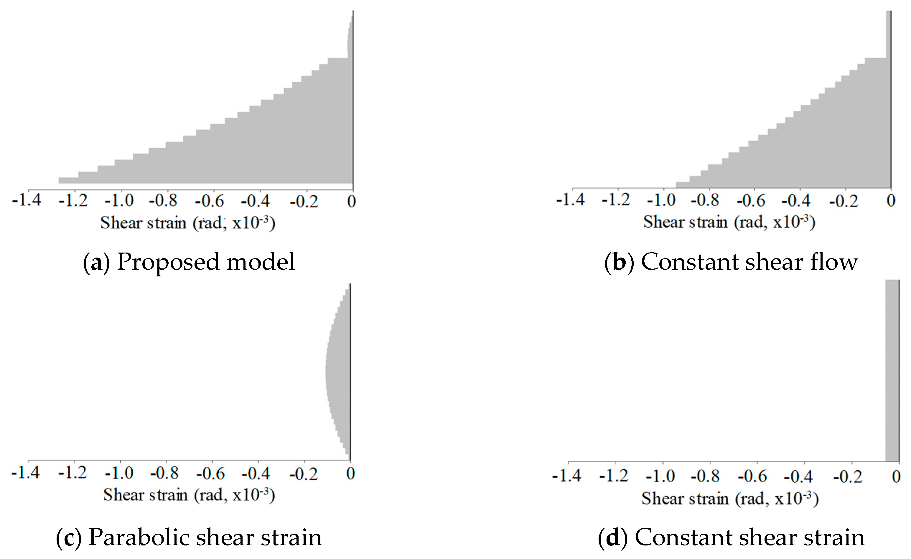
Figure 13 shows the shear strain distributions over the cross section at the same level of load. The proposed model described a parabolic shear distribution at the uncracked region (located top one-third portion), and dramatically increasing strains towards the bottom. Although a large discrepancy existed in the shear strain distributions, the contribution to the mid-span deflection of this seemed negligible. For example, the maximum shear strain estimated by the proposed model and the constant shear flow model were approximately 0.00135 and 0.00091, respectively, while the mid-span deflections were 2.54 mm and 2.79 mm, respectively. Their difference in maximum shear strain is 67% and that in mid-span deflection is 9%.

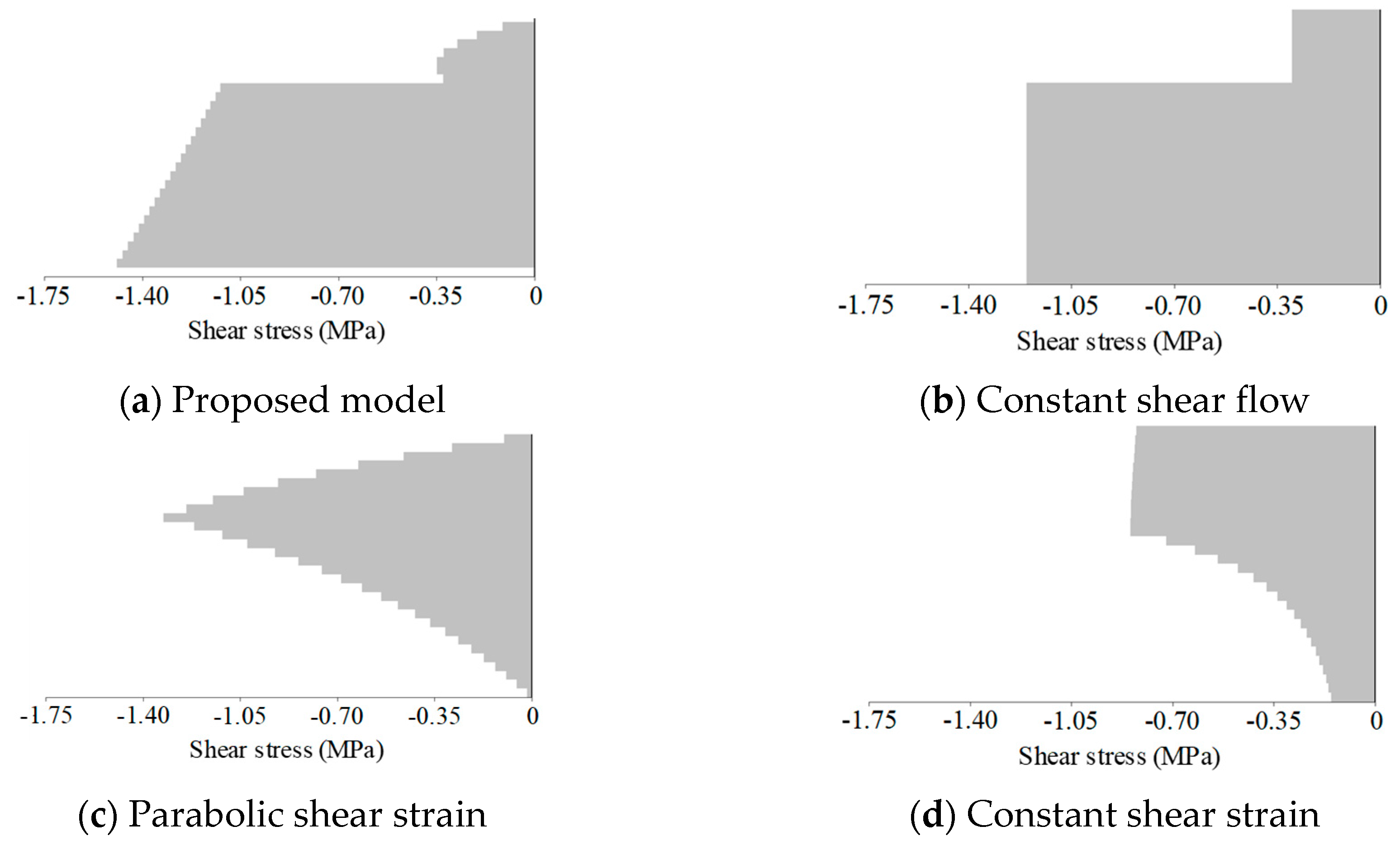
Figure 14 shows the shear stress distributions. The proposed model gave a similar shape of the shear stress distributions to that of the shear strain distribution; a parabolic shape in the uncracked region, and increasing stress towards the bottom. It is interesting to see the distributions obtained from the constant shear flow were similar to those from the proposed model. Together with the previous observations, this suggests that the constant shear flow model is a good approximation for the shear behavior of a reinforced concrete beam. In contrast, with the predefined shear strain models, a large portion of the shear stress residues are expected in the flange area. This may have reduced the shear stress in the web leading to the stiffer response.

10. Conclusions

In this study, the element formulation with the stress-driven shear force functions was derived and realized in the context of the finite element method. The proposed method showed excellent agreement with various RC beam test results. The two-dimensional representation of beam shear on the micro-plane successfully described the sectional shear stresses and strains, hence, allowing shear degradation and shear failure prediction in the global response. In addition, the coupled bending and shear behavior was accurately described, and the authors believe that in future studies, the axial load effects on shear behavior should be easily demonstrated, without any modification of the element formulation. In addition, since the formulation proposed in this study is very consistent with a strong applicability for nonlinear finite element analysis, it is expected that the proposed method can be applied to the existing finite element analysis software without interchangeability problems.

However, it is not clear at this point whether the incomplete post-peak response resulted from the inherent inconsistency in the element formulation. The inherent inconsistency may be ascribed to the use of the plane section assumption along with the stress-driven functions. Theoretically, the error due to this should disappear at convergence.