A Real-Time Numerical Decoupling Method for Multi-DoF Magnetic Levitation Rotary Table

Abstract

Magnetic levitation technology shows promise for realizing multiple degrees of free precision motion for modern manufacturing, as the bearing and guiding parts are not used. However, motion decoupling in a magnetically levitated (maglev) system is difficult because it is hard to derive accurate magnetic force and a torque model considering the translation and rotation in all axes. In this work, a magnetic levitation rotary table that has the potential to realize unlimited rotation around the vertical axis and a relatively long stroke in the horizontal plane is proposed and analyzed, and the corresponding real-time numerical decoupling method is presented. The numerical magnetic force and torque model solves the current to magnetic force and torque transformation matrix, and the matrix is used to allocate the exact current in each coil phase to produce the required motion in the magnetically levitated (maglev) system. Next, utilizing a high-level synthesis tool and hardware description language, the proposed motion-decoupling module is implemented on a field programmable gate array (FPGA). To realize real-time computation, a pipelined program architecture and finite-state machine with a strict timing sequence are employed for maximum data throughput. In the last decoupling module of the maglev system, the delay for each sampling point is less than $200\mathsf{\mu }$s. To illustrate and evaluate real-time solutions, they are presented via the DAC adapter on the oscilloscope and stored in the SD card. The error ratios of the force and torque results solved by the numerical wrench model were less than $5\%$ and $10\%$ using the solutions from the boundary element method (BEM) program package Radia^TM as a benchmark.

1. Introduction

A magnetically levitated (maglev) actuator is a promising substitute for a traditional electrical machine in modern industrial applications as it can provide accurate multiple degrees of freedom (DoF) movement benefiting from the characteristics of nonfriction and noncontact. This feature also decreases the vibration on the moving parts of the motion system because the transfer function between the displacements of the foundation and the levitation part has a low pass feature. Furthermore, the magnetic levitation system only contains a single moving part, so it possesses a compact design structure and wide control bandwidth. In the literature, taking advantage of maglev technology, there are the following five application scenarios related to intelligent instrumentation for modern industries:

• High-precision planar motion control to hold a wafer for a lithography machine [1,2].
• Providing multiaxis motion with resolution down to nanometers and microradian in less than a millimeter for nanoscale profiling and nanoindentation [3,4].
• Producing accurate force and torque in a large-volume region and unlimited rotation for haptic feedback systems [5,6].
• Used as actuator for magnetic manipulation for navigation or teleoperation systems in medical robots [7,8].
• Working as an active gravity compensator to reduce vibration for the stage [9,10].

Some researchers have explored maglev technology for the computerized numerical control (CNC) micromachine system, which always requires high-precision multiaxis motion in a certain working stroke [11]. The accuracy of the positioning system in these processing devices decides the manufacturing outcomes. In a traditional design, multi-DoF motion is realized via a rotary table assembled on a three-dimensional (3D) translational stage. However, in micromilling on the mesoscale, the resolution of the positioning system should be on the micro and microradian level in a range of several millimeters, and it is hard for ordinary translational equipment and rotary tables to meet these demands. Considering the existing positioning stage based on shape memory alloys (SMAs) and piezoelectric actuators [12], a magnetically levitated actuator is an alternative. Besides the advantage of accurate positioning ability, an electromagnetic actuator has a larger working stroke and a more linear performance compared with other micromotion devices. Furthermore, using the maglev actuator, micromachining CNC devices can miniaturize as there is only single moving part in the motion system. Therefore, a magnetically levitated rotary actuator with multi-DoF translational ability in a relative large stroke is studied in this work.

In general, the topology structure of maglev actuators is varied due to the real applications [13,14,15,16]. In an accurate motion-control area, a reasonable structure can not only decrease the force and torque ripples but also reduce difficulty in motion decoupling. The topology of the maglev rotary actuator can refer to the magnetically levitated planar motor [17,18] or employ the axisymmetric structure in which the magnet and coil are distributed along the circumference [11]. Once a specific design structure is given, the next step is obtaining the magnetic force and torque model [19,20,21,22,23,24,25]. It is also called the wrench model and is the foundation of the motion-decoupling unit in a control system. However, it is hard to consider the rotation angle and translation position in the existing modeling method at the same time, which hinders the maglev positioning system gaining translational rotational ability in a relatively large stroke [26]. In order to meet the requirements of micromachining on a mesoscale, it is necessary to study a suitable modeling method for motion decoupling in a large stroke.

Plenty of analytical force and torque modeling methods have been proposed for maglev system control. These wrench models should maintain computational accuracy and efficiency. In general, for large-stroke magnetic levitation positioning systems, the following three methods are often considered:

• Harmonic analysis method by solving Maxwell equations [27,28].
• Look-up table or curving fitting model using the measurements and results from finite-element method (FEM) software [29].
• Numerical method based on the basic law of electromagnetism [30,31,32].

The former two methods are mainstream in the literature because they are suitable for real-time computation, but their disadvantages are obvious. The harmonic analytical model cannot concurrently consider all motions and rotations, so large-range multi-DoF motion is hard to achieve. The look-up table and fitting model are built on the obtained force and torque dates, so generality is bad, and the multiaxis motion increases the stored data amount and decreases the accuracy of curving fitting. Furthermore, the numerical method is an alternative with its inherent generality, but it needs an advanced computation engineer to improve computation speed [33]. For a maglev system with a definite structure, a reasonable modeling method should be selected and studied.

In this work, a magnetic levitation rotary actuator with a novel topology structure is proposed that is able to synchronously realize translation and rotation. In order to model the electromagnetic actuator with both the translational and rotational position taken into account, magnetic force and torque are solved via the numerical method, as the magnetic charge model solves the magnetic flux density, and the Gaussian quadrature calculates the Lorenz integral. The magnetic field computation is also reasonably simplified to decrease the total computation burden. Additionally, because the proposed wrench model is required to realize motion decoupling, the real-time solution is realized via the field programmable gate array (FPGA) with a pipelined computation architecture. The computation delay for each sampling point is lower enough for the typical control system with $5\mathrm{kHz}$ control frequency. In the experiment section, real-time solutions are given on an oscilloscope and stored in an SD card. Modeling accuracy is evaluated due to a unified boundary element method (BEM) program package. Because the selected sampling points are located in a large region, the proposed numerical decoupling method is proved to be available to decouple the multiaxis motion in centimeters and amn unlimited rotating range, which is suitable for micromachining CNC devices used in the mesoscale.

2. Magnetic Levitation Rotary Table and Modeling Method

2.1. Working Principle of Maglev Actuator

The structure of the maglev actuator for the magnetic levitation rotary table is given in Figure 1. The rectangular permanent magnets and every two coils are symmetrical around the vertical axis. Additionally, the magnet array is formed in Halbach mode along the rotor circumference, and its geometric centers are located on a circle with radius R, as depicted in Figure 1a. Since there exist no contacts between stator and rotor, the motion system is able to undertake rotations and translations in all axes. Only the long side of each racetrack coil is located underneath the magnet array in the working stroke, so the moving range is decided by the size of the employed coils. Different from existing maglev rotary tables with the current in the coil radially flowing, this design, employing long racetrack coils, possesses the following advantages:

• This prototype is more suitable to realize translation in the horizontal plane because the area of one phase coil under the magnet array is constant when the rotor translates in the stroke.
• The design expense of the rotor is significantly reduced because it is not required to decrease the gap between the neighboring permanent magnets like the existing actuator in the maglev rotary table.
• The racetrack coil is easier to fabricate, install, and alter to other design parameters.

With the relative angles between coils and magnets varying when the system works, thrust and torsion ripples are more obvious compared with a traditional planar magnetically levitated actuator. Therefore, the accuracy of the force and torque model is more vital for stable motion control. Furthermore, as per the advantages of the design mentioned above, the structure of the coil set is not periodic along the argument, and the gap of the neighboring magnets in the array cannot be ignored. Therefore, traditional harmonic analysis cannot model an accurate magnetic-field distribution. In this work, the force and torque resulting from each coil are solved due to the magnetic charge method and Lorenz force integral independently.

To analyze the magnetic force and torque of each coil, several different coordinate systems $\left\{r\right\}$, $\left\{s\right\}$, $\left\{c_i\right\}$, and $\left\{m_j\right\}$, illustrated in Figure 1, are defined, which represent the rotor coordinate system, stator system, coil i, and magnet j coordinate system, respectively. The position and angle of the rotor are defined as a position and orientation vector (POV) ${}^s\mathbf{p}=\left({}^s{x}_r{,}^s{y}_r{,}^s{z}_r{,}^s{\alpha }_r{,}^s{\beta }_r{,}^s{\gamma }_r\right)$ in $\left\{s\right\}$. The x axis and y axis in $\left\{r\right\}$ or $\left\{s\right\}$ are parallel if the angles in ${}^s\mathbf{p}$ are equal to 0. Origins ${}^{r}o$ and ${}^{s}o$ are located at the top surface of the coil set and bottom surface of the magnet array, respectively, and ${}^{c_i}o$ and ${}^{m_j}o$ are the geometric centers of the corresponding coil and magnet. The position of each ${}^{c_i}o$ is determined by the design parameters of the known maglev system, and every origin point ${}^{m_j}o$ is located at a circle with radius R, shown in Figure 1a, when ${}^s{\gamma }_r$ is 0. Index i is from $0\sim 7$, while j is from $0\sim 47$. Furthermore, as shown in the top dashed block of Figure 1c, the ${}^{m_j}z-$ axis coincides with the remanence direction of the permanent magnet for magnetic field analysis due to the magnetic charge method [34]. Figure 1 also gives the design parameters of the coil and permanent magnet, as $w_c,r_c,l_c,h_c$ and $w_m,l_m,h_m$. The pitch angle of the Halbach array is $\frac{\pi }{24}$ with 48 permanent magnets existing in the rotor.

2.2. Force and Torque Computation

The resultant force and torque acting on the mover are from the magnetic interaction between the magnet array and all coils, and are defined as ${\left[{}^s{F}_x{,}^s{F}_y{,}^s{F}_z{,}^s{T}_x{,}^s{T}_y{,}^s{T}_z\right]}^{\mathrm{T}}$. The force and torque vector meets the equation below as the effects from the 8 coils need to be derived independently.

$$\left(\begin{array}{c}{}^s{F}_x\\ {}^s{F}_y\\ {}^s{F}_z\\ {}^s{T}_x\\ {}^s{T}_y\\ {}^s{T}_z\end{array}\right)=\left(\begin{array}{cccc}{}^s{F}_{x,0}& {}^s{F}_{x,1}& \cdots & {}^s{F}_{x,7}\\ {}^s{F}_{y,0}& {}^s{F}_{y,1}& \cdots & {}^s{F}_{y,7}\\ {}^s{F}_{z,0}& {}^s{F}_{z,1}& \cdots & {}^s{F}_{z,7}\\ {}^s{T}_{x,0}& {}^s{T}_{x,1}& \cdots & {}^s{T}_{x,7}\\ {}^s{T}_{y,0}& {}^s{T}_{y,1}& \cdots & {}^s{T}_{y,7}\\ {}^s{T}_{z,0}& {}^s{T}_{z,1}& \cdots & {}^s{T}_{z,7}\end{array}\right)·\left(\begin{array}{c}{I}_0\\ I_1\\ ⋮\\ I_7\end{array}\right)=\Gamma ·\mathbf{I},$$

(1)

where the current-wrench transformation matrix $\Gamma$ consists of eight force and torque vectors ${\left[{}^s{F}_{x,i}{,}^s{F}_{y,i}{,}^s{F}_{z,i}{,}^s{T}_{x,i}{,}^s{T}_{y,i}{,}^s{T}_{z,i},\right]}^{\mathrm{T}}$ representing the contribution from each coil, and $\mathbf{I}$ means the 8 phase current vectors containing the current in each coil. The transformation matrix is the foundation of motion decoupling in different directions and needs to be solved by the wrench model at each sampling cycle for allocating the phase current. To simplify the wrench vector of each coil, only the two long sides underneath the magnet array are considered in force and torque calculations. The magnetic force produced $\mathbf{Coili}$ is solved by

$${}^{{\mathrm{c}}_i}{\mathbf{F}}_i=-{\int }_{\frac{w_{\mathrm{c}}}{2}}^{\frac{w_{\mathrm{c}}}{2}+r_{\mathrm{c}}}{\int }_{-\frac{l_c}{2}}^{\frac{l_{\mathrm{c}}}{2}}{\int }_{-\frac{h_c}{2}}^{\frac{h_{\mathrm{c}}}{2}}{}^{{\mathrm{c}}_i}\mathbf{J}\times {}^{{\mathrm{c}}_i}\mathbf{B}d{}^{{\mathrm{c}}_i}zd{}^{{\mathrm{c}}_i}yd{}^{{\mathrm{c}}_i}x+{\int }_{-\frac{w_{\mathrm{c}}}{2}-r_{\mathrm{c}}}^{-\frac{w_{\mathrm{c}}}{2}}{\int }_{-\frac{l_c}{2}}^{\frac{l_{\mathrm{c}}}{2}}{\int }_{-\frac{h_c}{2}}^{\frac{h_{\mathrm{c}}}{2}}{}^{{\mathrm{c}}_i}\mathbf{J}\times {}^{{\mathrm{c}}_i}\mathbf{B}d{}^{{\mathrm{c}}_i}zd{}^{{\mathrm{c}}_i}yd{}^{{\mathrm{c}}_i}x,$$

(2)

where $\mathbf{J}$ and $\mathbf{B}$ represent the coil current density and magnetic flux density, and the upper and lower integral limitations are related to the design parameter of each coil.

2.2.1. Magnetic Force between Current-Carrying Region and Magnet

The proposed wrench model should be unified. Referring to the parallel wrench model proposed in a previous work [33], the magnetic force from one rectangular current-carrying region is solved due to the Lorenz integral through magnetic node, Gaussian quadrature, and coordinate transformation as

$${}^s{\mathbf{F}}_i=-{\sum }_{j=0}^{47}{\sum }_{g=0}^{G-1}{\sum }_{k=0}^7{\omega }_g·{}_{c_i}^s\mathbf{R}·{\mathbf{J}}_g\times {}_{c_i}^s{\mathbf{R}}^{-1}·{}_s^t{\mathbf{R}}^{-1}·{}_t^{m_j}{\mathbf{R}}^{-1}·{\mathbf{B}}_k\left\{{}_t^{m_j}\mathbf{R}·\left[{}_s^t\mathbf{R}·\left({}_{c_i}^s\mathbf{R}·{}^{c_i}{\mathbf{x}}_g+{}^s{\mathbf{o}}_{c_i}-{}^s\mathbf{d}\right)-{}^t{\mathbf{o}}_{m_j}\right]\right\},$$

(3)

where ${\mathbf{B}}_k$ {} represent the functions of solving a magnetic field excited by magnet node k using the object point positions as the input variables [34], ${}_1^2\mathbf{R}$ represents the rotation matrices from the coordinate systems $\left\{1\right\}$ to $\left\{2\right\}$, j represents the index of the magnet, g is the index of the Gaussian node in coil i, $J_g$ is the current density, ${\omega }_g$ is the multiple product of the three Gaussian weights in each order of volume integral, and ${}^s{\mathbf{o}}_{c_i}$ and ${}^t{\mathbf{o}}_{m_j}$ are the geometric centers of coil i and magnet j in coordinate system $\left\{s\right\}$ and $\left\{t\right\}$, respectively. The upper limitations of the summation, 47, G, and 7, represent the magnet amount, coil node amount, and magnet node amount in one magnet. Therefore, the summation item in this equation is the magnetic interaction between a single coil node and a single magnet node. The input variable ${}^{c_i}{\mathbf{x}}_g$ is the position of the coil node, as shown in Figure 1c. With the index g known, its position is calculated depending on the index in each integral order as below.

$${}^{c_i}{\mathbf{x}}_g=\left({}^{c_i}{x}_g{,}^{c_i}{y}_g{,}^{c_i}{z}_g\right)=\left(\frac{1}{2}\left(l_c+r_c\right)·{\lambda }_{g1},\frac{1}{2}{w}_c·{\lambda }_{g2}\pm \frac{w_c+r_c}{2},\frac{1}{2}{h}_c·{\lambda }_{g3}\right),$$

(4)

where $g_1$, $g_2$, and $g_3$ are the order of Gaussian quadrature meeting the relationship in Equation (5):

$$g=4·g_1+2·g_2+2·g_3-1.$$

(5)

A + or − operation in $\pm \frac{w_c+r_c}{2}$ is decided by the integral region location. Orders of Gaussian quadrature are defined as 2 in the integral over ${}^{c_i}y$ and ${}^{c_i}z$ and 4 in the integral over ${}^{c_i}x$, respectively, and the corresponding Gaussian node and weight are given in

Table 1. Gaussian node and weight for two-order and four-order Gaussian quadrature.

Order Number	2-Order		4-Order
Gaussian node	${\omega }_0=1.0$	${\omega }_1=1.0$	${\omega }_0=0.348$	${\omega }_1=0.652$	${\omega }_2=0.652$	${\omega }_3=0.348$
Gaussian weight	${\lambda }_0=-0.577$	${\lambda }_1=0.577$	${\lambda }_0=-0.861$	${\lambda }_1=-0.334$	${\lambda }_2=0.334$	${\lambda }_3=0.861$

. The order can be set to another number as a larger order number for better computation accuracy, but it also results in a greater computation burden [19].

The rotation matrices in Equation (3) are obtained due to the rotation angle, as ${}_s^{c_i}\mathbf{R}$ and ${}_s^t\mathbf{R}$ are

$$\mathbf{R}\left({\theta }_z\right)=\left(\begin{array}{ccc}\cos {\theta }_z& -\sin {\theta }_z& 0\\ \sin {\theta }_z& \cos {\theta }_z& 0\\ 0& 0& 1\end{array}\right),$$

(6)

where ${\theta }_z$ is the rotation angle around the corresponding vertical axis. As illustrated in Figure 1a, the rotation angle of $\mathbf{Coil}\mathbf{0},\mathbf{1}$, $\mathbf{Coil}\mathbf{2},\mathbf{3}$, $\mathbf{Coil}\mathbf{4},\mathbf{5}$, $\mathbf{Coil}\mathbf{6},\mathbf{7}$ are 0, $\frac{\pi }{2}$, $\pi$, and $\frac{3\pi }{2}$, respectively, which are equal to $\mathbf{floor}\left(\frac{i}{2}\right)·\frac{\pi }{2}$, where the $\mathbf{floor}$ means the round-down operation. The ${\theta }_z$ for the ${}_s^t\mathbf{R}$ is ${}^s\gamma$ in the POV vector. The rotation matrix ${}_t^{m_j}\mathbf{R}$ is written as

$$\mathbf{R}\left({\theta }_z\right)=\left(\begin{array}{ccc}1& 0& 0\\ 0& \cos {\theta }_x& -\sin {\theta }_x\\ 0& \sin {\theta }_x& \cos {\theta }_x\end{array}\right)·\left(\begin{array}{ccc}\cos {\theta }_z& -\sin {\theta }_z& 0\\ \sin {\theta }_z& \cos {\theta }_z& 0\\ 0& 0& 1\end{array}\right).$$

(7)

Because the ${}^{m_j}z$ axis is along the remanence direction, as given in Figure 1c, it should rotate around the ${}^{m_j}z$ axis and then around the ${}^{m_j}x-$ axis. Referring to the design structure of the Halbach array, ${\theta }_z$ is $\frac{\pi }{24}·j$ and ${\theta }_x$ is decided by the index number of the magnet as Equation (8), where $\mathbf{mod}$ () means the modulo operation.

$${\theta }_x=\mathbf{mod}\left(j,4\right)\times \frac{\pi }{2}$$

(8)

Once force is obtained, the torque can be solved by cross-multiplying the force solution with the arm moment. The magnetic force from a coil is equivalent to acting on the rotor just above the coil center, so the arm moment relates to the position component in POV vector ${}^s\mathbf{p}$ and the location of the coil center in the stator. Thus, the magnetic torque from coil i is solved by Equation (9):

$${}^s{\mathbf{T}}_i=\left({}_{c_i}^s\mathbf{R}·{\left(R,\Delta w,0\right)}^{\mathrm{T}}-\left({}^s{x}_r{,}^s{y}_r,0\right)\right)\times {}^s{\mathbf{F}}_i,$$

(9)

where $\Delta w$ is equal to ${\left(-1\right)}^i·\left(r_c+\frac{w_c}{2}\right)$.

2.2.2. Permanent Magnet Selection Law for Magnetic Force Computation

Based on superposition theory, magnetic flux density $\mathbf{B}$ in Equation (3) contains the results from all magnets in the rotor, where j is from 0 to 47. However, if all magnets are taken into account, the computation burden becomes huge, so real-time computation is hard to achieve. Because the magnetic field intensity produced by the permanent magnet at a certain point is inversely proportioned to the square of the distance between this point and the permanent magnet center, the magnets are not considered in the wrench model if they produce a magnetic field intensity less than $3\%$ of the magnetic field from the nearest magnet to this point. Under this circumstance, the deviation angle of the current-carrying region, given as ${\theta }_e$ and related to the rotary table is used as the standard for selecting the permanent magnets. The deviation angle of each long side of a coil is solved by

$${\theta }_e\left(i\right)=-{}^s{\gamma }_r+\mathbf{floor}\left(\frac{i}{2}\right)·\frac{\pi }{2}-\Delta d÷R,$$

(10)

where R is the radius given in Figure 1, $\mathbf{floor}\left(\frac{i}{2}\right)·\frac{\pi }{2}$ represents the rotation angles of each coil coordinate system $\left\{c_i\right\}$ referring to the $\left\{s\right\}$ coordinate system, and $\Delta d$ is the distance between original point ${}^{r}o$ and the central line of each long side. In order to choose the suitable magnets in the magnetic field computation, Figure 2 is introduced for the analysis. As illustrated in Figure 2a, $\Delta d$ is ${-}^s{y}_r+1.5·r_c+w_c$ if the right long side of $\mathbf{Coil}\mathbf{5}$ is considered.

Meanwhile, the intensity of the magnetic flux density produced by the red magnet in Figure 2a is explored to decide the reasonable magnet amount used in the wrench model. The testing points are located $2\mathrm{mm}$ below the bottom surface of the permanent magnet and distributed at the red circumference in this figure. Results are shown in Figure 2b, where the space between each testing point is the pitch angle $\frac{\pi }{24}$. Observing the results, the magnetic intensity at the fourth point referring to the 0 degree point is less independent of the remanence direction of the permanent magnets. Therefore, the 7 nearest magnets to the current-carrying region, indicated by $j-3,j-2,j-1,j,j+1,j+2,j+3$, are selected for force computation in this work. The permanent magnet index n is solved by Equation (11):

$$j=\left\{\begin{array}{ccc}\mathrm{mod}\left({\theta }_e\left(i\right),\frac{\pi }{24}\right)& \mathbf{if}& \mathbf{floor}\left({\theta }_e\left(i\right),\frac{\pi }{24}\right)\le \frac{\pi }{48}\\ \mathrm{mod}\left({\theta }_e\left(i\right),\frac{\pi }{24}\right)+1& \mathbf{if}& \mathbf{floor}\left({\theta }_e\left(i\right),\frac{\pi }{24}\right)>\frac{\pi }{48}\end{array}\right.,$$

(11)

where $\mathbf{mod}$ () and $\mathbf{floor}$ () are the modulo function and round-down function, as mentioned before. With such a selecting law, the permanent magnets required to compute the force vector for a certain coil are decided due to Equation (11) after the POV ${}^s\mathbf{p}$ is obtained from the sensing system in the real prototype.

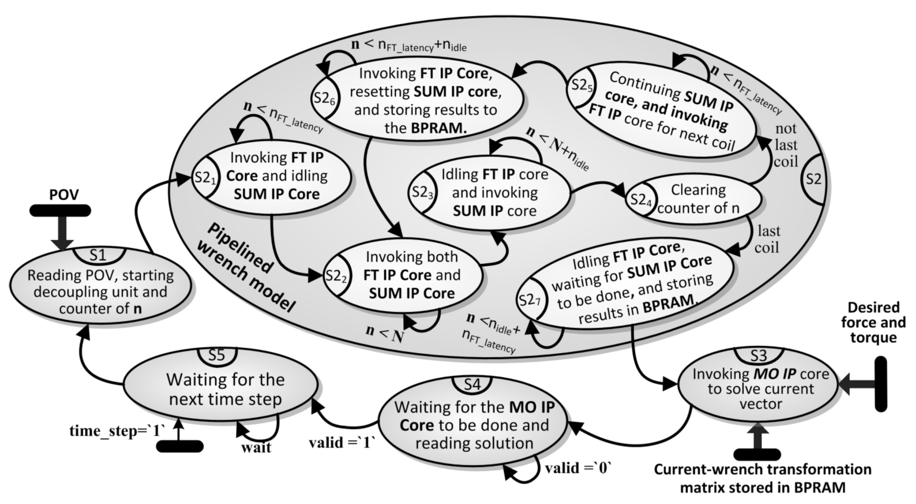
3. Real-Time Decoupling Unit Implemented on FPGA

3.1. Implementation on FPGA via High-Level Synthesis (HLS) Tool

The matched controller of the maglev system regulates the currents on each coil phase to produce the required magnetic force and torque for the desired movement. Because the contribution of each coil contains different force and torque components, the solution of the proposed wrench model, the current–wrench transformation matrix $\Gamma$, is necessary to decouple force and torque in different directions by reasonably distributing the current of each coil. Current vector $\mathbf{I}$ is solved by Equation (12):

$$\mathbf{I}={\Gamma }^{\mathrm{T}}·{\left(\Gamma ·{\Gamma }^{\mathrm{T}}\right)}^{-1}·{\mathbf{w}}_{\mathrm{desire}},$$

(12)

where ${\mathbf{w}}_{\mathrm{desire}}$ represents the desired force and torque from the control algorithm at each sampling cycle, which is a $6\times 1$ column vector written as ${\left[{}^s{F}_x{,}^s{F}_y{,}^s{F}_z{,}^s{T}_x{,}^s{T}_y{,}^s{T}_z\right]}^{\mathrm{T}}$. Additionally, these computation tasks should be implemented in the real control system, as illustrated in Figure 3. In this case, the magnetically levitated stage is equivalent to six independent second-order systems, so six independent single-input single-output (SISO) linear control algorithms, such as PID or the lead-lag method, can be used in the design.

On the other hand, for implementation in the real controller, the processing delay of the proposed numerical decoupling unit needs to be less than the sampling cycle of the controller. Observing Equation (12), the decoupling unit contains two parts, calculating the transformation matrix $\Gamma$ and the matrix operation, including matrix inversion and multiplication. Obtaining $\Gamma$ due to the numerical wrench model is time-consuming because it requires many computations. Normal single-thread processors, like the digital signal processor, processor with ARM (Advanced RISC Machines) architecture, or real-time kernel, cannot realize real-time processing with numerous computation branches. Under this circumstance, the FPGA is considered because of the high working frequency and flexible hardware reconfiguration. Evaluating the features of the wrench model given in Equation (3), the pipelined program structure is suitable to realize computation. Meanwhile, the FPGA is not only convenient to interface with the device, such as the AD–DA adapter and data bus, but is also able to construct the built-in processor to run the control algorithm. Therefore, in this work, the FPGA is employed as the computation platform for the real-time current decoupling unit for the maglev rotary actuator.

In general, programs running on FPGA are the digital circuits in a register-transfer level (RTL) structure designed by a hardware description language (HDL). The programming language directly manipulates the register like the assembler language, which is suitable for the timing sequence control and bus design, but it is difficult and error-prone to lay out the complicated algorithm for dates in a floating-point type. Xilinx^® has introduced the High-Level Synthesis (HLS) ^TM tool to directly translate a C specification into an RTL implementation. As a highly abstract language, C++ has many library functions, so the coding effort for floating-point data processing is substantially reduced compared with HDL. The optimization methods of RTL implementation contain the pipeline, loop unroll, and array partition, and are provided in the HLS tool, which is helpful for developing computation efficiency. The C++ program for the numerical wrench model and the matrix operation is exported as RTL components and can be invoked as the intellectual property (IP) core in FPGA projects.

3.2. Current Decoupling Unit Implementation

The numerical decoupling process is given in the left flowchart of Figure 4. The dashed block represents the summation item in Equation (3) using the POV ${}^s\mathbf{p}$, coil index i, and loop index n as input variables. In the program, the loop amount is N estimated by the coil node number in one coil times the magnet node number:

$$N=1792=2\times 2\times 2\times 4\times 7\times 8,$$

(13)

where the first 2, the middle $2,2,4$, the following 7, and the last 8 respectively represent the two integral regions for one coil, the coil node amount in each integral region, the required magnet number for a magnetic field solution, and the magnetic node number in the cubic permanent magnet. Then, the force and torque solution are summed up to obtain the current–wrench transformation matrix $\Gamma$ for the later matrix operation of Equation (12). Through the HLS^TM tool, the summation item in Equation (3) and the matrix operation in Equation (12) are exported as a FT (Force & Torque) IP core and MO (Matrix Operation) IP core. As the aforementioned derived wrench model shares the same expression with different input variables, it is suitable to work with the pipelined architecture. In order to develop throughput, the interval for the pipelined FT IP core should be 1 so that the processing of each loop is independent from the others and cannot contain the for statement. Force and torque solutions of the same coil are summed up, and the summation is the wrench vector in $\Gamma$. Therefore, six independent SUM IP cores from Logicore^TM are also required for the corresponding summing operation. Finally, the MO IP core is employed to calculate the current vector for the desired force and torque, in which the Gaussian elimination realizes the matrix inversion operation. The matrix operation is also optimized by the internal pipeline and array partition in the HLS^TM tool to maintain latency and computation resources.

The entire decoupling unit was designed based on these RTL modules on the FPGA platform shown in the middle column of Figure 4. The module in the dashed block was used for the numerical wrench model realized by the IP cores and a counterproducing loop index n and coil index i. The solutions from the FT IP core should be sent to the SUM IP core, also owing to a pipelined architecture, one by one. The final results from the SUM are stored in a bipolar RAM constructed in FPGA whose other side directly connects with the MO IP core. The outputs of the FT IP core are actually continuous due to the pipelined structure, so the timing sequence of the data communication between each IP core should be elaborately designed or the solution will be faulty. As illustrated in the right column of Figure 4, if all of loop index n for one coil is accomplished, there exists an idle clock for the next coil. The reason is that SUM IP cores are required to reset for the wrench vector computation of the next coil. Observing the timing sequence flow, the total delay clock of the numerical wrench model for the magnetically levitated rotary actuator is estimated below.

$$n_{\mathrm{wm}\_\mathrm{latency}}=n_{\mathrm{FT}\_\mathrm{lantency}}+n_{\mathrm{SUM}\_\mathrm{lantency}}+7\times n_{\mathrm{idle}}+8\times N,$$

(14)

where $n_{\mathrm{FT}\_\mathrm{lantency}}$, $n_{\mathrm{MO}\_\mathrm{lantency}}$, and $n_{\mathrm{SUM}\_\mathrm{lantency}}$ represent the inherent delay of FT, MO, SUM IP cores, N is number of computation units for the wrench vector of each coil, and $n_{\mathrm{idle}}$ is the idle clock after all variables for one coil having been sent to the FT IP core. The $n_{\mathrm{idle}}$ is larger than $n_{\mathrm{sum}\_\mathrm{lantency}}$ as the SUM IP core should reset after the wrench vector computation for one coil is accomplished. Once the current–wrench transformation matrix $\Gamma$ is obtained, the MO IP core is started, and then the FPGA RTL implementation will wait for the end of the matrix operation. Therefore, the total delay of the decoupling unit is given by

$$T_{\mathrm{delay}}=T_{\mathrm{clk}}\times \left(n_{\mathrm{wm}\_\mathrm{latency}}+n_{\mathrm{MO}\_\mathrm{latency}}\right),$$

(15)

where $T_{\mathrm{clk}}$ means the clock period of the FPGA. As this module is required to be inserted in the controller for the maglev rotary actuator, the $T_{\mathrm{delay}}$ should be less than the sampling cycle of the control system.

The state machine given in Figure 5 introduces the layout in detail. State S1 reads POV ${}^s\mathbf{p}$ and starts the counter. Then, State S2, presenting the pipelined program structure, begins. In these states, ${\mathbf{S}\mathbf{2}}_1$∼${\mathbf{S}\mathbf{2}}_5$, both the FT IP core and SUM IP core are invoked and idle with a certain timing sequence. In State ${\mathbf{S}\mathbf{2}}_6$, counter n needs to be cleared for the next coil computation, the SUM IP core should reset, and results of SUM IP core are stored in the bipolar RAM. Inversely, the FT IP core cannot be reset like the SUM IP core because its latency is very long. If the FT IP core has finished the force and torque calculation for the last coil, the state machine switches from ${\mathbf{S}\mathbf{2}}_4$ to ${\mathbf{S}\mathbf{2}}_7$ and waits for the accomplishment of the summing operation. After that, State S3 reads the required wrench vector and invokes the MO IP core. With the current vector solved in State S4, the program goes to S5, waiting for the next time step. With reconfigurable characteristics, the RTL structure for the decoupling unit can be implemented on the arbitrary FPGA platform with enough computation resources.

4. Experiment Results

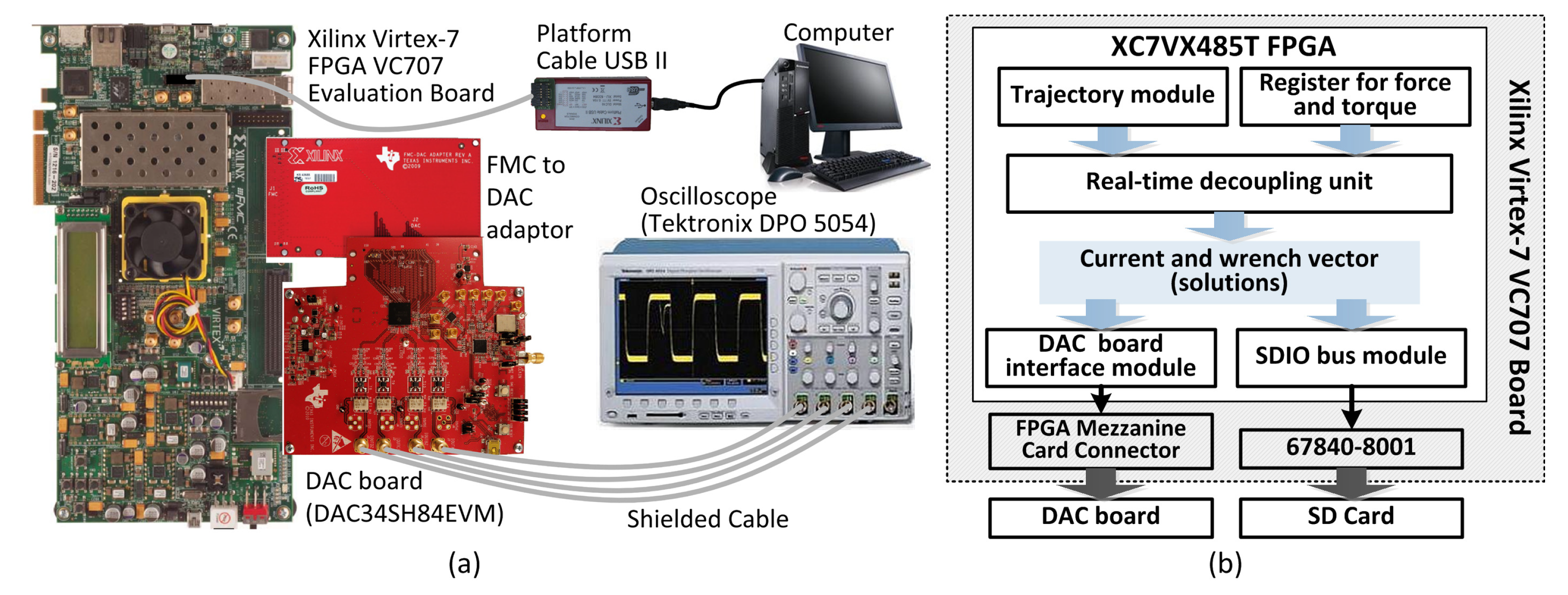
4.1. Experiment Setup

The numerical current decoupling unit was implemented on the Xilinx^® Virtex-7 VC707 Evaluation Board as given in Figure 6a. In FPGA implementation, except for the necessary aforementioned IP cores, the DAC (Digital to analog converter)board interface module and the SDIO (Secure digital input and output) bus module were also designed. The two modules can display and store a real-time solution on the oscilloscope and SD card, respectively. In the test, the moving part of the maglev system was emulated to move along the trajectory, given as Equation (16), in which the units of translations and rotations are millimeters and radians, respectively, so the system works in a large translational and rotational stroke. Thus, the trajectory module was also inserted into the implementation, as shown in Figure 6b.

The real-time solution contains elements in the current–wrench matrix and the obtained current values for a desired force and torque vector. The data are displayed as the waveform on the oscilloscope via the DAC board. As there are only four channels on the oscilloscope, the displayed solutions are selected by a dual in-line pin (DIP) package switch. Additionally, these displayed dates should be transformed from a single floating-point format to a fixed-point format, then adjusted to LVDS (Low-Voltage differential signaling) format and sent in DDR (Double data rate)mode.

$${}^s\mathbf{p}={\left({}^{s}x{,}^{s}y{,}^{s}z{,}^s\alpha {,}^s\beta {,}^s\gamma \right)}^{\mathrm{T}}={\left(15\cos \left(4\pi t\right),10\sin \left(4\pi t\right),0.5+2t,0,0,10\pi t\right)}^{\mathrm{T}}$$

(16)

The design parameters given in

Table 2. Design parameters for the magnetically levitated rotary actuator shown in Figure 1.

Parameter	${\mathit{l}}_{\mathit{c}}$	${\mathit{w}}_{\mathit{c}}$	${\mathit{r}}_{\mathit{c}}$	${\mathit{h}}_{\mathit{c}}$	${\mathit{l}}_{\mathit{m}}$	${\mathit{w}}_{\mathit{m}}$	${\mathit{h}}_{\mathit{m}}$	Remanence	Coil Turns
Value	$60\mathrm{mm}$	$10\mathrm{mm}$	$10\mathrm{mm}$	$10\mathrm{mm}$	$30\mathrm{mm}$	$8\mathrm{mm}$	$8\mathrm{mm}$	$1.2\mathrm{T}$	300

are employed in the layout of the RTL current decoupling module on FPGA. As analyzed in (13), the amount of the computation unit is $14,336$. The latency of the FT and MO IP cores is 254 and 3756, respectively, referring to the HLS report, while the latency of the SUM IP core is 4 and the idle time between each coil solution is 10 clocks in the layout. Therefore, the time period is $184.2\mathsf{\mu }\mathrm{s}$ with the $100\mathrm{MHz}$ main frequency on the FPGA evaluation board. In this case, the sampling frequency would be $5\mathrm{kHz}$ for the real-time decoupling unit.

The maglev system was also modeled with a program package running on Mathematic^® named Radia^TM. This program package is a boundary element analysis tool, and solutions are used to evaluate the validation of the real-time solutions. Next, the current–wrench transformation matrix and the obtained current solutions are shown and compared.

4.2. Validation of the Real-Time Wrench Model and Current Decoupling Unit

To evaluate the computation accuracy of the numerical wrench model, the solutions of all coils in the coil set were solved and shown on an oscilloscope, assuming the mover in the maglev system takes motion along the trajectory of Equation (16) for $0.1$ s. In each subfigure of Figure 7, the left column shows the force components, and the right shows the torque components in the current–wrench transformation matrix. With a $5\mathrm{kHz}$ sampling frequency, there were 501 sampling points on each waveform. As the boundary method is very time-consuming, only 101 sampling points were calculated here. In this figure, the waveform and the BEM results are very approximate. To quantitatively analyze the accuracy of the proposed real-time numerical wrench model, the relative error ratios of the wrench vector from the FPGA were calculated using BEM results as the benchmark.

Table 3. Relative error of force and torque solutions for each coil using BEM results as a benchmark.

Error Ratio	Coil 0	Coil 1	Coil 2	Coil 3	Coil 4	Coil 5	Coil 6	Coil 7
${\eta }_{\mathbf{F}}$	$4.16\%$	$4.53\%$	$2.95\%$	$$5.05\%$$	$2.21\%$	$4.89\%$	$3.91\%$	$3.78\%$
${\eta }_{\mathbf{T}}$	$8.98\%$	$8.32\%$	$6.59\%$	$8.43\%$	$9.39\%$	$5.49\%$	$5.84\%$	$5.36\%$

shows the average relative error of the resultant force and torque considering the 101 sampling points in the BEM model via Equation (17):

$$\left({\eta }_{\mathbf{F}},{\eta }_{\mathbf{T}}\right)=\frac{1}{100}\sum _{\mathrm{point}=0}^{101}\left(\frac{∥{\mathbf{F}}_{\mathrm{wm},\mathrm{point}}-{\mathbf{F}}_{\mathrm{BEM},\mathrm{point}}∥}{∥{\mathbf{F}}_{\mathrm{BEM},\mathrm{point}}∥},\frac{∥{\mathbf{T}}_{\mathrm{wm},\mathrm{point}}-{\mathbf{T}}_{\mathrm{BEM},\mathrm{point}}∥}{∥{\mathbf{T}}_{\mathrm{BEM},\mathrm{point}}∥}\right)\times 100\%,$$

(17)

where ${\mathbf{F}}_{\mathrm{wm}}$ , ${\mathbf{T}}_{\mathrm{wm}}$, and ${\mathbf{F}}_{\mathrm{BEM}}$ , ${\mathbf{T}}_{\mathrm{BEM}}$ are the resultant force and torque produced by each coil via the numerical wrench model or the BEM software at each sampling point, respectively. Observing the results in Table 3, we concluded that the force and torque error were not beyond $5\%$ and $10\%$, which highlights that the real-time numerical wrench model has a similar computation accuracy compared with the BEM for the magnetically levitated rotary actuator.

In order to test the real-time current decoupling unit, the magnetically levitated rotary actuator is assumed to provide a force and torque vector, $\left[0\mathrm{N},0\mathrm{N},20\mathrm{N},0\mathrm{N}·\mathrm{mm},0\mathrm{N}·\mathrm{mm},200\mathrm{N}·\mathrm{mm}\right]$, acting on the rotor when it moves along the trajectory of (16) in $0.5$ s. The current results for each coil are illustrated as waveforms in Figure 8. Meanwhile, the decoupling current estimated by the BEM solutions are also given as dots in this figure. The real-time numerical current decoupling unit results are not only close to the ones from the off-line emulator, but also can be employed in the controller directly for current regulation in each phase of the coil set.

Furthermore, the obtained current value is substituted in the BEM model to solve the magnetic force and torque produced at the corresponding sampling points. In Figure 9, the 101 real-time current solutions shown in Figure 8 are used as the exciting current in the BEM model to calculate force and torque values. The simulation results were approximated to the desired force and torque, which also proves the validation of the real-time current decoupling unit.

4.3. Computation Resource

The RTL implementation processing the floating-point data always spends many hardware resources in FPGA. Here, the required hardware resources and the occupation ratio, containing the look-up table (LUT), Flip Flop (FF), and digital signal processor (DSP), are given in

Table 4. FPGA resource utilization for hardware implementation. DPSs—digital signal processors; FF—Flip Flop; LUT— look-up table.

FPGA Resources	Current Decoupling Module		Data Displaying and Storing Modules
	Wrench Model	Matrix Operation	Trajectory	DAC Connector	SDIO Driver
LUT	$\mathrm{45,672}(15.04\%)$	$5664(1.87\%)$	$6433(2.12\%)$	$1606(0.53\%)$	$869(0.29\%)$
FF	$\mathrm{38,806}(6.39\%)$	$9329(1.54\%)$	$4546(0.75\%)$	$680(0.11\%)$	$502(0.08\%)$
DSPs	$245(8.75\%)$	$76(2.71\%)$	$56(2.00\%)$	$16(0.57\%)$	$0(0.0\%)$

for each module. The current decoupling unit contains two parts: the numerical wrench model and matrix operation. The former is constructed by the FT and SUM IP cores, and the latter uses the MO IP core. The trajectory, display, and data-storing module for testing also consumes some resources. The total occupied computation resources are not beyond $20\%$. Thus, there are enough spare resources for the next control algorithm design. Low resource occupation benefits from the pipelined RTL structure in which only one numerical FT IP core is employed. Meanwhile, as only the 7 nearest magnets to the current-carrying region were selected for force and torque computation, the computation burden significantly decreases. Computation efficiency can further develop if more FT IP cores are employed in the implementation. However, referring to the existing magnetic levitation system, we assumed that the $5\mathrm{kHz}$ sampling frequency is high enough for the design of the matching controller.

5. Discussion of FPGA-Based Numerical Current Decoupling Unit for Magnetically Levitated Rotary Actuator

The FPGA-based numerical current decoupling unit for the maglev actuator is based on the numerical wrench model and the matrix operation module. The experiments prove the effectiveness of the current decoupling RTL component in two aspects. First, the solutions of the numerical wrench model were compared with the unified BEM program package Radia^TM. The error ratios of the results from the numerical wrench model were not beyond $5\%$ and $10\%$, and these results were assumed to reflect the real performance of the maglev actuator. Second, the current vector solved by the current decoupling unit was substituted in the boundary element model to evaluate validity. Even if there exists some force and torque ripples in the simulation results, these deviations could be inhibited by the feedback control in the real magnetic levitation system.

Computation efficiency and the occupied computation resources of the decoupling unit affect its application in the real controller. Referring to the computation unit amount calculated by Equation (13) and the synthesis reports from HLS^TM, the computation delay was less than $200\mathsf{\mu }$s, which is high enough for the sampling cycle of a real maglev system controller. Furthermore, the data given in Table 4 also show that the implementation of the decoupling unit is not a burden for the existing FPGA evaluation board. In future work, the magnetically levitated rotary table will be fabricated, and the multi-DoF motion controller will be constructed based on the proposed FPGA-based current decoupling unit.

6. Conclusions

An FPGA-based real-time current decoupling unit for a prototype of a magnetically levitated rotary actuator was proposed in this work. In the decoupling process, the numerical wrench model was capable of solving the current–wrench transformation matrix when the actuator undertook multiple DoF motions. Then, the current for each coil was solved by the matrix operation for the desired force and torque at a certain position. Computation accuracy was evaluated by comparing the real-time solutions with the offline BEM programming package, Radia^TM, and the low relative error highlighted the validity of the numerical wrench model and the decoupling unit. Computation efficiency and occupied resources were also discussed in the experiment, and it was concluded that the obtained RTL decoupling unit is available for the real controller used in the maglev prototype.

References

1. Jansen, J.W.; Van Lierop, C.M.M.; Lomonova, E.A. Magnetically Levitated Planar Actuator with Moving Magnets. IEEE Trans. Ind. Appl. 2008, 44, 1108–1115. [Google Scholar] [CrossRef]
2. Hu, C.; Wang, Z.; Zhu, Y.; Zhang, M.; Liu, H. Performance-Oriented Precision LARC Tracking Motion Control of a Magnetically Levitated Planar Motor With Comparative Experiments. IEEE Trans. Ind. Electron. 2016, 63, 5763–5773. [Google Scholar] [CrossRef]
3. Kim, W.J.; Verma, S.; Shakir, H. Design and precision construction of novel magnetic-levitation-based multi-axis nanoscale positioning systems. Prec. Eng. 2007, 31, 337–350. [Google Scholar] [CrossRef]
4. Zhang, Z.; Menq, C.H. Six-Axis Magnetic Levitation and Motion Control. IEEE Trans. Robot 2007, 23, 196–205. [Google Scholar] [CrossRef]
5. Tong, Q.; Yuan, Z.; Liao, X.; Zheng, M.; Yuan, T.; Zhao, J. Magnetic Levitation Haptic Augmentation for Virtual Tissue Stiffness Perception. IEEE Trans. Vis. Comput. Graph. 2018, 24, 3123–3136. [Google Scholar] [CrossRef] [PubMed]
6. Pedram, S.A.; Klatzky, R.L.; Berkelman, P. Torque contribution to haptic rendering of virtual textures. IEEE Trans. Haptics 2017, 10, 567–579. [Google Scholar] [CrossRef] [PubMed]
7. Pieters, R.; Tung, H.W.; Charreyron, S.; Sargent, D.S.; Nelson, B.J. RodBot: A Rolling Microrobot for Micromanipulation. In Proceedings of the IEEE International Conference on Robotics and Automation (ICRA), Seattle, WA, USA, 26–30 May 2015; pp. 4042–4047. [Google Scholar]
8. Casson, J.; O’Kane, S.; Smith, C.A.; Dalby, M.; Berry, C. Interleukin 6 plays a role in the migration of magnetically levitated mesenchymal stem cells spheroids. Appl. Sci. 2018, 8, 412. [Google Scholar] [CrossRef]
9. Xu, F.; Xu, X.; Chen, M. Prototype of 6-DOF Magnetically Levitated Stage Based on Single Axis Lorentz force Actuator. J. Electr. Eng. Technol. 2016, 11, 1216–1228. [Google Scholar] [CrossRef] [Green Version]
10. Zhang, H.; Kou, B.; Jin, Y.; Zhang, H. Modeling and Analysis of a New Cylindrical Magnetic Levitation Gravity Compensator With Low Stiffness for the 6-DOF Fine Stage. IEEE Trans. Ind. Electron. 2015, 62, 3629–3639. [Google Scholar] [CrossRef]
11. Dyck, M.; Lu, X.; Altintas, Y. Magnetically Levitated Rotary Table with Six Degrees of Freedom. IEEE/ASME Trans. Mechatron. 2017, 22, 530–540. [Google Scholar] [CrossRef]
12. Ouyang, P.R.; Tjiptoprodjo, R.C.; Zhang, W.J.; Yang, G.S. Micro-motion Devices Technology: The State of Arts Review. Int. J. Adv. Manuf. Technol. 2008, 38, 463–478. [Google Scholar] [CrossRef]
13. Yuan, L.; Zhang, J.; Chen, S.; Liang, Y.; Chen, J.; Zhang, C. Design and Optimization of a Magnetically Levitated Inductive Reaction Sphere for Spacecraft Attitude Control. Energies 2019, 12, 1553. [Google Scholar] [CrossRef]
14. Zhang, H.; Kou, B. Design and Optimization of a Lorentz-Force-Driven Planar Motor. IEEE Trans. Magn. 2007, 23, 196–205. [Google Scholar] [CrossRef]
15. Zhang, S.; Huang, J.; Yang, J. Raising Power Loss Equalizing Degree of Coil Array by Convex Quadratic Optimization Commutation for Magnetic Levitation Planar Motors. Appl. Sci. 2019, 9, 79. [Google Scholar] [CrossRef]
16. Wang, Y.; Chen, X.; Luo, X.; Zhang, L. Analysis and Optimization of a Novel 2-D Magnet Array with Gaps and Staggers for a Moving-Magnet Planar Motor. Sensors 2018, 18, 124. [Google Scholar] [CrossRef] [PubMed]
17. Ueda, Y.; Ohsaki, H. A Planar Actuator with a Small Mover Travelling Over Large Yaw and Translational Displacements. IEEE Trans. Magn. 2008, 44, 609–616. [Google Scholar] [CrossRef]
18. Lu, X.; Usman, I.U.R. 6D Direct-drive Technology for Planar Motion Stages. CIRP Ann.-Manuf. Technol. 2012, 61, 359–362. [Google Scholar] [CrossRef]
19. Xu, F.; Lv, Y.; Xu, X.; Dinavahi, V. FPGA-Based Real-Time Wrench Model of Direct Current Driven Magnetic Levitation Actuator. IEEE Trans. Ind. Electron. 2018, 65, 9635–9645. [Google Scholar] [CrossRef]
20. Kou, B.; Xing, F.; Zhang, L.; Zhang, C.; Zhou, Y. A Real-Time Computation Model of the Electromagnetic Force and Torque for a Maglev Planar Motor with the Concentric Winding. Appl. Sci. 2017, 7, 98. [Google Scholar] [CrossRef]
21. Xing, F.; Kou, B.; Zhang, L.; Yin, X.; Zhou, Y. Design of a Control System for a Maglev Planar Motor Based on Two-Dimension Linear Interpolation. Energies 2017, 10, 1132. [Google Scholar] [CrossRef]
22. Jansen, J.W.; Smeets, J.P.C.; Overboom, T.T.; Rovers, J.M.M.; Lomonova, E.A. Overview of Analytical Models for the Design of Linear and Planar Motors. IEEE Trans. Magn. 2014, 50, 8206207. [Google Scholar] [CrossRef]
23. Castellanos, M.L.; Galluzzi, R.; Bonfitto, A.; Tonoli, A.; Amati, N. Magnetic Levitation Control Based on Flux Density and Current Measurement. Appl. Sci. 2018, 8, 2545. [Google Scholar] [CrossRef]
24. Jeyasenthil, R.; Choi, S.B. A Robust Controller for Multivariable Model Matching System Utilizing a Quantitative Feedback Theory: Application to Magnetic Levitation. Appl. Sci. 2019, 9, 1753. [Google Scholar] [CrossRef]
25. Lahdo, M.; Ströhla, T.; Kovalev, S. Repulsive magnetic levitation force calculation for a high precision 6-DoF magnetic levitation positioning system. IEEE Trans. Magn. 2017, 53, 7020106. [Google Scholar] [CrossRef]
26. Yuan, D.; Zhang, M.; Zhu, Y.; Li, X.; Wang, L. Demonstrating the Potential of a Hybrid Model to Increase the 360 Degrees Rotational Motion Freedom of Ironless Permanent Magnet Planar Motors. In ASME International Mechanical Engineering Congress and Exposition; V010T13A007; American Society of Mechanical Engineers: New York, NY, USA, 2018. [Google Scholar]
27. Zhu, Y.; Yuan, D.; Zhang, M.; Liu, F.; Hu, C. Unified wrench model of an ironless permanent magnet planar motor with 2D periodic magnetic field. IET Electr. Power Appl. 2017, 12, 423–430. [Google Scholar] [CrossRef]
28. Jansen, J.W.; Van Lierop, C.M.M.; Lomonova, E.A.; Vandenput, A.J.A. Modeling of Magnetically Levitated Planar Actuators With Moving Magnets. IEEE Trans. Magn. 2007, 43, 15–25. [Google Scholar] [CrossRef]
29. Estevez, P.; Mulder, A.; Schmidt, R.H.M. 6-DoF Miniature Maglev Positioning Stage for Application in Haptic Micro-manipulation. Mechatronics 2012, 22, 1015–1022. [Google Scholar] [CrossRef]
30. Xu, F.; Peng, R.; Zheng, T.; Xu, X. Development and Validation of Numerical Magnetic Force and Torque Model for Magnetically Levitated Actuator. IEEE Trans. Magn. 2019, 55, 4900109. [Google Scholar] [CrossRef]
31. Xu, F.; Xu, X.; Li, Z.; Chu, L. Numerical Calculation of the Magnetic Field and Force in Cylindrical Single-Axis Actuator. IEEE Trans. Magn. 2014, 50, 7200506. [Google Scholar] [CrossRef]
32. Peng, J.; Zhou, Y.; Liu, G. Calculation of a New Real-time Control Model for the Magnetically Levitated Ironless Planar Motor. IEEE Trans. Magn. 2013, 49, 1416–1422. [Google Scholar] [CrossRef]
33. Xu, F.; Dinavahi, V.; Xu, X. Parallel Computation of Wrench Model for Commutated Magnetically Levitated Planar Actuator. IEEE Trans. Ind. Electron. 2016, 63, 7621–7631. [Google Scholar] [CrossRef]
34. Bancel, F. Magnetic Nodes. J. Phys. D Appl. Phys. 1999, 32, 2155–2161. [Google Scholar] [CrossRef]
Figure 1. Structure of a magnetically levitated (maglev) actuator for six degrees of freedom (DoF) magnetic levitation rotary table: (a) Top view of coil set in stator and magnet array in rotor with corresponding coordinate system, (b) side view of coil set and magnet array, (c) partial view of one coil and two permanent magnets with a coil coordinate system and magnet coordinate system.
Applsci 09 03263 g001
Figure 2. (a) Diagram of the actuator to analyze the relative angle θ e of Coil 5 in the rotor coordinate system. (b) Intensity of magnetic flux density along the testing arc line from Magnet 0 in (a) .
Applsci 09 03263 g002
Figure 3. Control block of the magnetic levitation rotary table with force and torque decoupling unit. SISO—single-input single-output.
Applsci 09 03263 g003
Figure 4. Flowchart, design structure, and timing sequence diagram of the current decoupling unit on the field programmable gate array (FPGA) platform. POV—position and orientation vector.
Applsci 09 03263 g004
Figure 5. Finite-state machine of current decoupling based on numerical wrench model and matrix operation.
Applsci 09 03263 g005
Figure 6. (a) Computation and displaying device for the implementation of numerical current decoupling for the magnetically levitated rotary actuator; (b) necessary computation modules in register-transfer level (RTL) structure and peripheral device for evaluation board.
Applsci 09 03263 g006
Figure 7. Waveform of real-time solutions on the oscilloscope (up) and boundary element method (BEM) solution obtained by RadiaTM (down). (ah) Results of Coil 0Coil 7, respectively.
Applsci 09 03263 g007
Figure 8. Current results of the proposed real-time current decoupling unit (line) and the off-line BEM simulation program (dots).
Applsci 09 03263 g008
Figure 9. Magnetic force and torque simulation results solved by RadiaTM using current solutions from the real-time numerical current decoupling unit shown in Figure 8.
Applsci 09 03263 g009