Design and Validation of a Self-Driven Joint Model for Articulated Arm Coordinate Measuring Machines

Abstract

Articulated arm coordinate measuring machines (AACMMs) have been developed and applied in industrial measurement fields for more than 30 years. Manual operation is typically required during measurement, which introduces uncertain influences, such as fluctuation of measurement force, speed, and acceleration, and leads to poor reliability and reproducibility. In this paper, a novel self-driven joint model is proposed to realize automatic measurement for AACMMs. A self-driven joint is designed by combining the joint of an AACMM with a robotic arm to realize automatic rotation. A self-driven AACMM is designed using three rolling joints and three pitching joints with assigned parameters. A virtual prototype of the self-driven AACMM is established using the Adams software to simulate the driving moment of each joint. The simulation results demonstrate that the designed mechanical structure and selected devices can meet the preset requirements. Additionally, based on the proposed model, a single physical joint is developed and assembled for performance testing. Experimental results demonstrate that the model can achieve a repeatability of 1.39″ (k = 2) when the rotational velocity is less than 1.53 rad/s. Therefore, the proposed design is suitable for use in AACMMs.

1. Introduction

Traditional articulated arm coordinate measuring machines (AACMMs) are widely used in industrial fields based on their portability, wide measuring space, and low cost. The key technologies of articulated coordinate measuring machines were instrument structure, error analysis, measurement model, eccentric error correction of circular grating installation, development of standard components for parameter calibration or performance evaluation of AACMM, optimization of parameter calibration algorithm, etc. [1]. Methods for improving the accuracy of AACMMs largely focus on kinematics modeling and the calibration of structural parameters [2,3,4,5,6,7]. AACMMs have complex error performance. The structural parameter error of AACMMs cannot be avoided in the manufacturing process. It is necessary to identify the structural parameters through parameter calibration to enhance AACMMs measurement accuracy. A kinematic calibration procedure normally consists of four steps: determination of the kinematic model, data acquisition for calibration, parameter identification using calibration data, and experimental validation [8]. The Denavit-Hartenberg (DH) approach or the modified Denavit-Hartenberg (MDH) approach is widely employed to establish a kinematic model [9,10,11,12]. The coupling relationship between kinematic parameters was considered and obtained via the singular value decomposition before the identification and compensation models were established [12]. Quaternions are another way of describing rotation in three dimensions. Battista et al. [13] introduced a kinematic model established by quaternions. Data acquisition is carried usually out by using various artifacts, for example, a 3D artifact [14] was composed of 14 reference points with three different heights, another example was a kind of ball bar used for length reference that calibration tests were carried out in larger space by changing ball bar pose [7,11]. Acero R. et al. [15] used a laser tracker as a reference instrument for AACMM calibration and verification procedures. The technique increases the flexibility for defining test positions. In general, parameter calibration is performed using a mathematical method to process the sampled data. It is important to select optimization methods. Cheng et al. [8] compared the nonlinear least method, genetic algorithm method, and simulated annealing method. Experimental results show that nonlinear least square method is very suitable for parameter identification of AACMM and is widely used [10,11,12,13,16]. The sampled data was processed for the exclusion of rough error [11]. Interior point method was used to identify the structural parameters of AACMM and has no requirement on the iterative initial value, which can effectively improve the success rate of parameter calibration [17].

Moreover, researchers summarize error sources and try to compensate them to improve the performance of AACMM. Santolaria et al. [18] and Luo et al. [19] tried to compensate for temperature error. The temperature error correction models were established on the basis of the kinematic model established at 20 °C by using the experimental modeling method that found out the variation of the structural parameters at other temperature and added the variation to the corresponding parameters. Yu et al. [20] and Vrhovec et al. [21] developed laser measurement systems to acquire the deformation of the serial mechanism link. Deformations due to external forces were measured and corrected. Probe errors of coordinate measuring arm were studied [22,23]. Luo et al. [22] studied the error source and influencing factors of the probe, and a mathematical model by the simulated annealing method of the relationship between the equivalent diameter and the measuring force of the AACMM was built to compensate for the equivalent diameter error of the probe caused by the measuring force. Virtual articulated arm coordinate measuring machines were developed for the determination of measurement results along with its uncertainty [24,25]. The uncertainty of the measurement point for an AACMM was modeled by ellipsoids [24]. Zheng et al. [26] measured a workpiece using an AACMM and found that the length measurement accuracy of the workpiece was not the same in different positions within the measuring space. The optimal measurement area, that is, the area with the highest accuracy, is supposed to exist in the whole measuring space. The optimal measuring area is related to the error characteristics of the angle measuring system. An ant colony algorithm was used to determine the optimal measurement area for an AACMM [27].

However, random errors introduced by users cannot be controlled to ensure an optimal trajectory, constant force measurement, and stable contact direction. González-Madruga et al. [28] stated that AACMMs lacked traceability and reliability, which was largely based on human error, but the error was not considered in current measurement and evaluation methods. Cuesta et al. [29,30] pointed out that AACMM errors related to human factors were caused by non-uniform contact forces, lack of stability, different velocities, and accelerations, among unpredictable probing trajectories, resulting in unpredictable structural deformation during the AACMM measurement process. AACMMs utilize a manual drag-and-drop measurement mode. Although this method avoids complicated path planning and control problems, it also introduces uncontrollable measurement force, random measurement posture, uneven sampling points, poor repeatability and stability [29], and inapplicability to production lines or the online automatic measurement.

Therefore, this paper proposes a self-driven joint module for constructing self-driven articulated arm coordinate measuring machines. Based on theoretical analysis, a virtual prototype of a self-driven AACMM is established by using the MSC Adams 2016 software for simulation analysis and component selection. A physical single-joint prototype was developed and feasibility experiments were carried out. The proposed self-driven AACMM makes it possible to perform measurements with optimal measurement attitudes, in which grating sensor measurement error and machine deformation error are less.

2. Design of the Joint Module

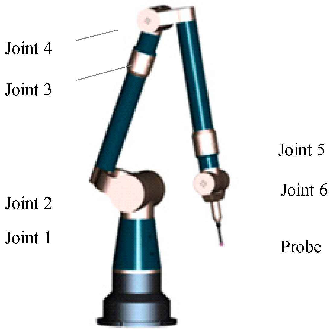
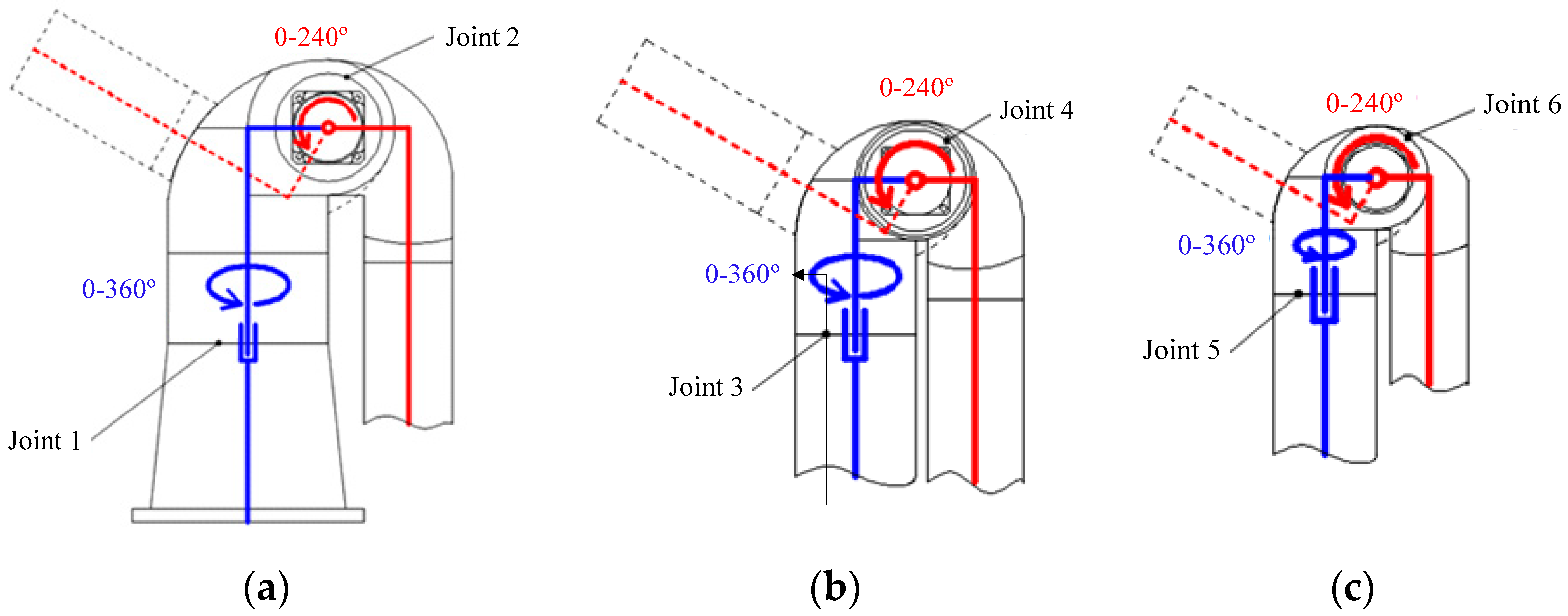
2.1. Joint Configurations

The joint structures of typical AACMMs and robotic arms are compared below. (1) AACMMs utilize precision shaft and encoder systems that are small and lightweight. (2) Robotic arms, which are drive oriented to ensure smooth movement and a higher deceleration ratio, typically use a motor and harmonic reducer to drive joints. (3) The encoder installation in an AACMM is placed near the joint output with high accuracy based on its measurement purpose, whereas the encoder precision of a robotic arm is typically lower because the encoder is installed at the back of the motor for control purposes. (4) The output of a robotic arm is directly connected to the reducer, and the concentricity between the bearing and harmonic reducer is required to be high. (5) The joints in a robotic arm can be divided into two main types of configurations, namely rolling and pitching joints. Similarly, Joints 1, 3, and 5 in an AACMM are rolling joints, while Joints 2, 4, and 6 are pitching joints, as shown in Figure 1.

Figure 1. Structure of an articulated arm coordinate measuring machine (AACMM).

We designed joints model for a self-driven AACMM based on the advantages of existing AACMMs and robotic arms, as shown in Figure 2.

Figure 2. Joint model for a self-driven AACMM [31].

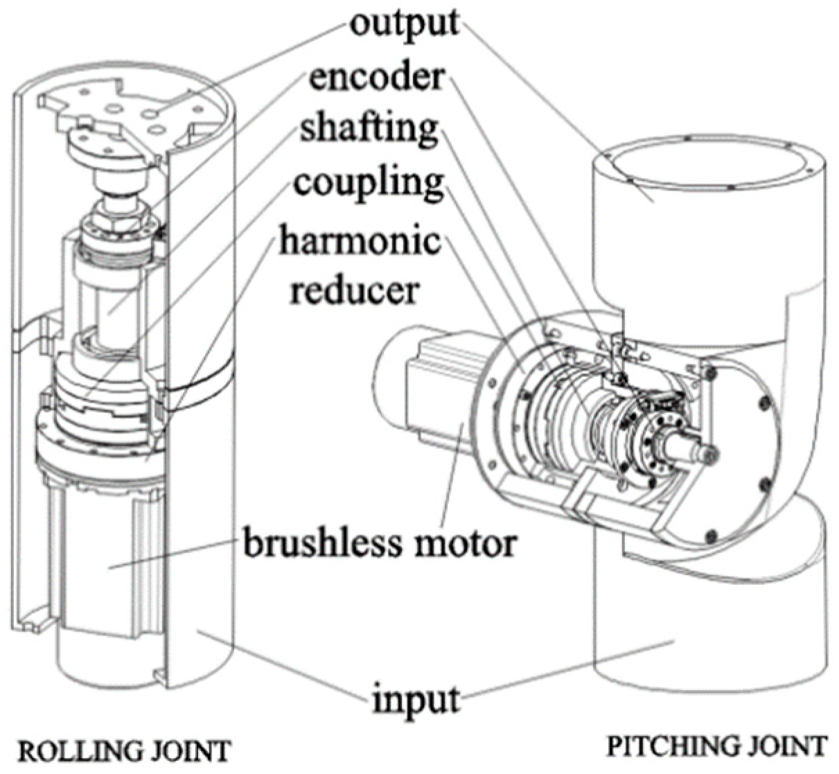
2.2. Joint Part Selection

The main parameters for the proposed self-driven AACMM are listed below. (1) The total length is no less than 1.2 m. (2) The angular accelerations of Joints 1 and 2 do not exceed 10°/s². Those of Joints 3 and 4 do not exceed 20°/s². Those of Joints 5 and 6 do not exceed 30°/s². (3) The load on Joint 6 is the constant force trigger probe. The load on other joint modules comes from the weight attached to its output end to the probe part. Analysis of the driving force of the joint model for the self-driven AACMM can be conducted by referring to the following dynamics equation from the field of robotics [32]:

$$Q=M(q)\ddot{q}+C(q,\dot{q})\dot{q}+F(\dot{q})+G(q),$$

(1)

where, q is the position vector of the joint, $\dot{q}$ is the joint velocity vector, $\ddot{q}$ is the joint acceleration vector, $M(q)$ is the mass matrix, $C(q,\dot{q})$ is a matrix related to Coriolis acceleration and centripetal acceleration, $F(\dot{q})$ is a vector related to viscous friction and coulomb friction, $G(q)$ is a moment vector by the presence of gravity, and Q is the generalized moment vector.

Based on the low movement speed of the arm, $C(q,\dot{q})$ in Equation (1) can be ignored. The influence of the friction term $F(\dot{q})$ can also be ignored. Therefore, Equation (1) can be simplified as follows:

$$Q=M(q)\ddot{q}+G(q).$$

(2)

Equation (2) indicates that the driving moment required by the self-driven joint module is related to its own mass, rotational angular acceleration and load. The required joint’s moment can be expressed by

$$Q=M_{\mathrm{M}}+M_{\mathrm{J}},$$

(3)

where, M_M is the static moment on the joint introduced by its load and M_J is the moment required to change the motion state of the joint itself and load.

Based on Equation (3) and the AACMM structure, design, and component selection were carried out by calculating each step from the probe to the base in a preliminary study [31]. Table 1 lists the design parameters, and load moment for each joint, and minimum moment required for the motor and reducer. Table 2 lists the parameters of the brushless motor and reducer.

Table 1. Results of motor torsion estimation [31].

Joint/Parameter	Joint 1	Joint 2	Joint 3	Joint 4	Joint 5	Joint 6	Probe
Total mass (g)	5555	6586	6043	4448	4034	3344	1087
Centroid distance (mm)	140	450	130	380	100	150	-
Angular acceleration (°/s2)	10	10	20	20	30	30	-
Maximum inertia moment (N·m)	20.04	18.17	6.46	6.37	0.20	0.16	-
Maximum load moment by gravity (N·m)	0.00	136.31	38.49	38.49	1.60	1.60	-
Peak moment (N·m)	20.04	154.48	44.95	44.86	1.94	1.90	-
Deceleration ratio	120	120	100	100	50	50	-
Minimum moment required for motor (N·m)	0.17	1.29	0.45	0.45	0.04	0.04	-

Table 2. Primary parameters for the motor and reducer.

		Joint 1/Joint 2	Joint 3/Joint 4	Joint 5/Joint 6
Motor	Rated moment (N·m)	1.6	0.5	0.1
	Mass (g)	1800	1050	500
Harmonic reducer	Mass (g)	1240	560	380
	Peak moment (start/stop) (N·m)	159	51	17
	Maximum moment (instant) (N·m)	289	104	33

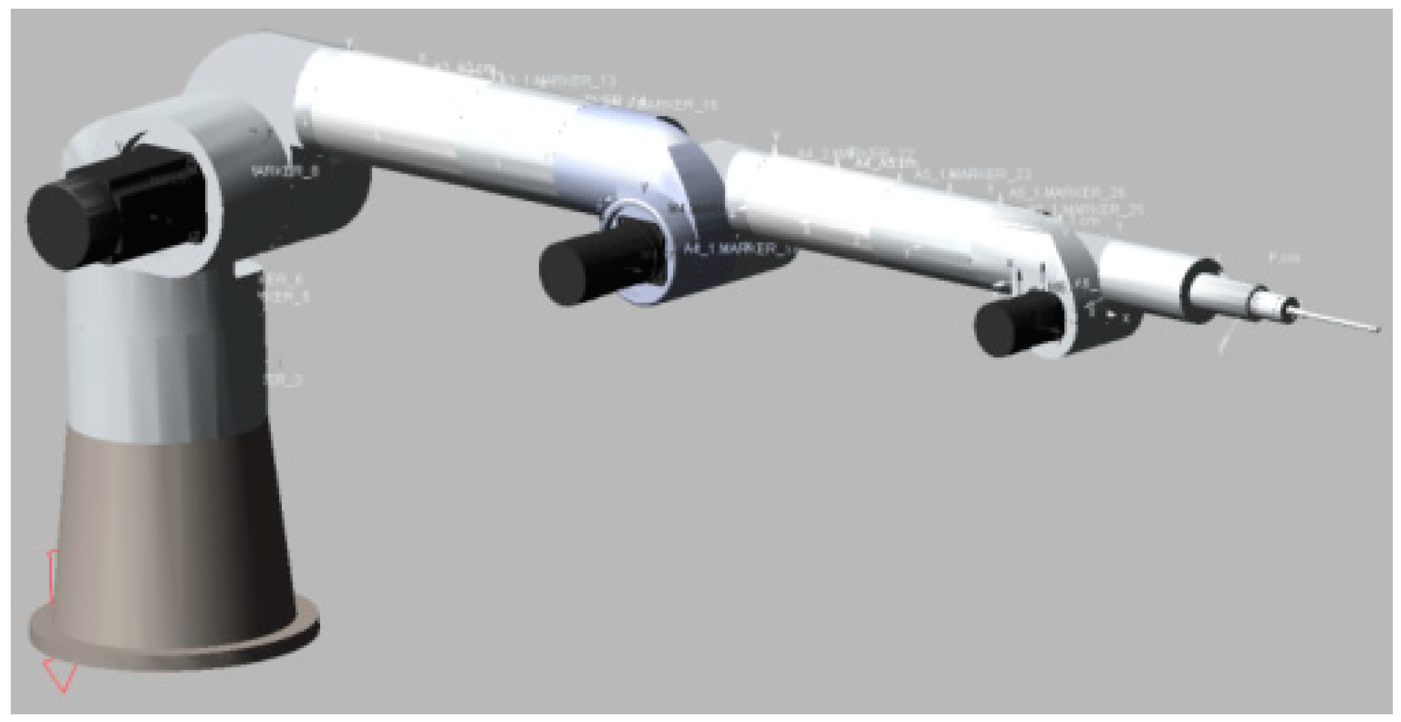
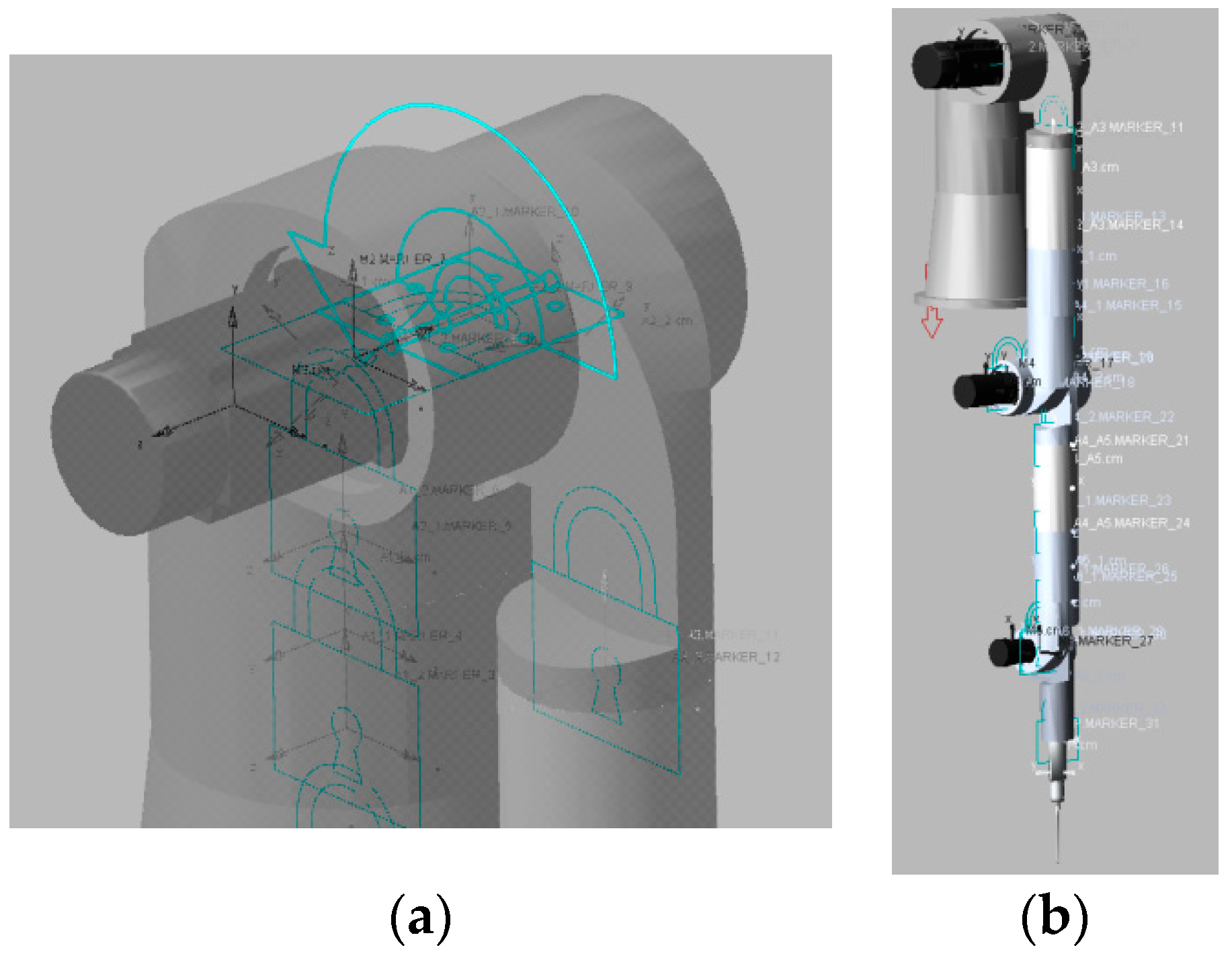
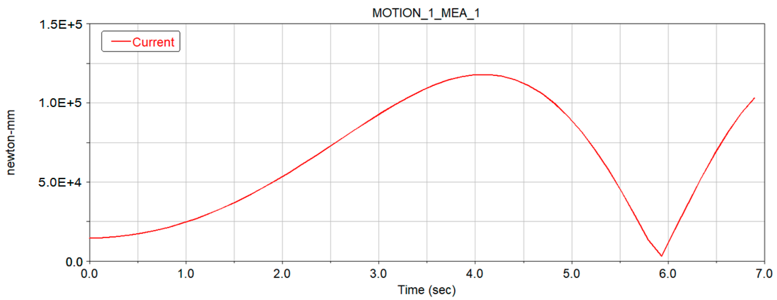
2.3. Virtual Prototype Construction and Moment Simulation

Virtual prototyping technology is a novel computer-aided engineering technology that enables design analysis through simulations of all or part of the physical prototype functions on the platform [33]. In this study, SolidWorks 2015 3D CAD software was used for modeling, and MSC Adams was used to establish a virtual prototype of the self-driven AACMM. The moment curves of the joints were obtained through computer simulations of machine motion, and the selections listed above were verified.

By combining the pitching and rolling joint configurations in Figure 2 with the primary parameters in Table 1, a 3D model was designed in SolidWorks. A distribution diagram of each part is presented in Figure 3. For the convenience of MSC Adams simulation, an effective merging of the parts to create a model of the self-driven AACMM was performed.

Figure 3. 3D model of the self-driven AACMM.

(1)

The cylindrical radii of the rotating parts of the joints in the model were set to the ideal cylindrical radii.

(2)

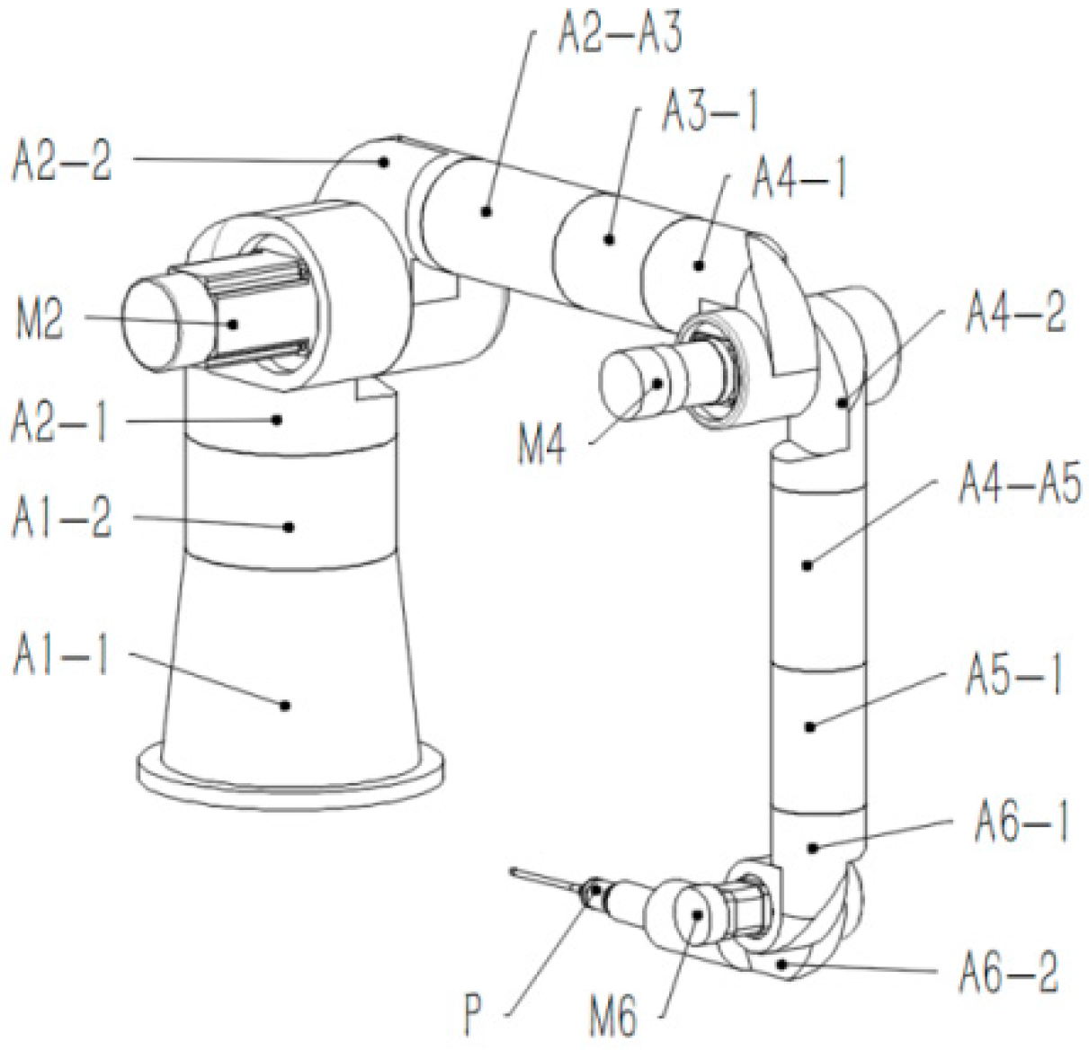
The output portion of Joint 1 was merged with the input portion of Joint 2, the output portion of Joint 3 was merged with the input portion of Joint 4, and the output portion of Joint 5 was merged with the input portion of Joint 6.

(3)

Joints 1 and 2 (excluding Motor 2) constituted a union with uniform density. The masses of the input and output parts of Joints 1 and 2 were distributed proportionally to their proportions of the total volume of the union.

(4)

Joints 3 (not including the front connecting rod) and 4 (excluding Motor 4) constituted a union with uniform density. The masses of the input and output parts were also distributed according to their volume proportions.

(5)

Joints 5 and 6 were treated the same as Joints 3 and 4.

(6)

The output portion of Joint 6 and the measuring head constituted a union with uniform density. Again, the component mass was distributed according to the volume proportions.

The components of the 3D model following mass distribution are listed in Table 3. The angle ranges and hinge relationships of Joints 1 and 2, 3 and 4, and 5 and 6 are presented in Figure 4.

Table 3. 3D part mass distribution.

Part Index	Part Name	Part Mass (g)	Volume (cm3)	Volume Ratio (%)	Model Mass (g)	Model Density (g/cm3)
A1-1	Joint 1 input (including Motor 1)	10,610	6627.71	42.52	5154	0.78
A1-2	Joint 1 output		2544.69	16.33	1979
A2-1	Joint 2 input		3729.58	23.93	2900
A2-2	Joint 2 output		2684.65	17.22	2089
M2	Motor 2 (including brake)	2100	849.22	100	2100	2.47
A2-A3	Joint 2–3 link rod	293	164.56	100	293	1.78
A3-1	Joint 3 input (including Motor 3)	7023	942.48	30.53	2144	2.28
A4-1	Joint 4 input		1336.23	43.29	3040
A4-2	Joint 4 output		808.29	26.18	1839
M4	Motor 4 (including brake)	1250	270	100	1250	4.63
A4-A5	Joint 4–5 link rod	200	112.48	100	200	1.78
A5-1	Joint 5 input (including Motor 5)	5290	628.32	56.37	2982	4.75
A6-1	Joint 6 input		486.30	43.63	2308
A6-2	Joint 6 output	1087	622.10	89.50	973	1.56
P	Probe		73.00	10.5	114
M6	Motor 6 (including brake)	700	121.64	100	700	5.75

Figure 4. Schematic diagram of the angle ranges and hinge relationships of each joint, they should be listed as: (a) Description of what is Joints 1 and 2, (b) Description of what is Joints 3 and 4, (c) Description of what is Joints 5 and 6.

In SolidWorks, the shape of each part was designed, and the densities of the components in the material configuration were set to the entity densities calculated in Table 3. The final 3D model was fabricated as an assembly and saved as an x_t file. When creating a new model in MSC Adams and choosing to import the generated x_t file, the 3D model is imported into the MSC Adams model as an entity. Figure 5 presents the 3D model of the self-driven AACMM.

Figure 5. 3D model imported in MSC Adams View.

The 3D model imported into MSC Adams inherits the spatial location, entity volume, centroid coordinates, and custom density from the SolidWorks environment. The initial position of the model after it is imported into MSC Adams is the same as that in SolidWorks, but assembly relationships are no longer enforced, and the corresponding constraints between joints and the ground must be added according to the rotation relationships between joints.

First, the Joint 1 input was fixed to the ground. We then attached a fixed hinge to the ground and added a rotating hinge for Joint 2. The axis of rotation was set to the center axis of the motor, and the remaining joints were connected using another fixed hinge, as shown in Figure 6a. For Joint 2, regarding MSC Adams hinge motion (joint motion), a column shape was selected for rotational motion. The selected shape was then added to a rotating hinge, and the added drive property was edited to ensure constant angular acceleration. To accomplish this, the property type was set to acceleration, and the angular acceleration value was set as 10°/s² (0.1745 rad/s²). The rest joints were locked with fixed hinges, and the initial pose of the model simulation is shown in Figure 6b.

Figure 6. Simulation model for the self-driven AACMM, they should be listed as: (a) Description of what is Constraints and motion of Joint 2, (b) Description of what is initial pose.

We set the simulation time to 6.9 s, meaning Joint 2 will rotate from 0° to 240°, and set the compensation to 100 steps to complete the simulation. The simulated moment curve is presented in Figure 7, where the maximum moment is 118.11 N·m.

Figure 7. 3D model imported in MSC Adams View.

The moment curves of the other joints were also obtained through MSC Adams simulation. The maximum values of the curves are listed in Table 4, and the maximum moment values that each joint can provide by Table 2 are listed in the last two columns of Table 4. Comparing and analyzing the data in Table 4, we conclude that the selected motor and reducer meet the system requirements. However, there are some discrepancies between design and simulation, and we believe there is still room for further structural optimizations and weight reduction. Using MSC Adams to perform virtual prototyping simulations can provide important references for such optimizations.

Table 4. Comparison of moments between the MSC Adams simulation of six joints and idea model.

Joint	Angular Acceleration (°/s2)	Peak Moment (MSC Adams) (N·m)	Peak Moment of Reducer (Start/Stop) (N·m)	Output Moment of Motor with Reducer (N·m)
1	10	12.42	159	192
2	10	118.11	159	192
3	20	38.26	51	50
4	20	31.77	51	50
5	30	1.97	17	5
6	30	0.84	17	5

3. Experiments and Results

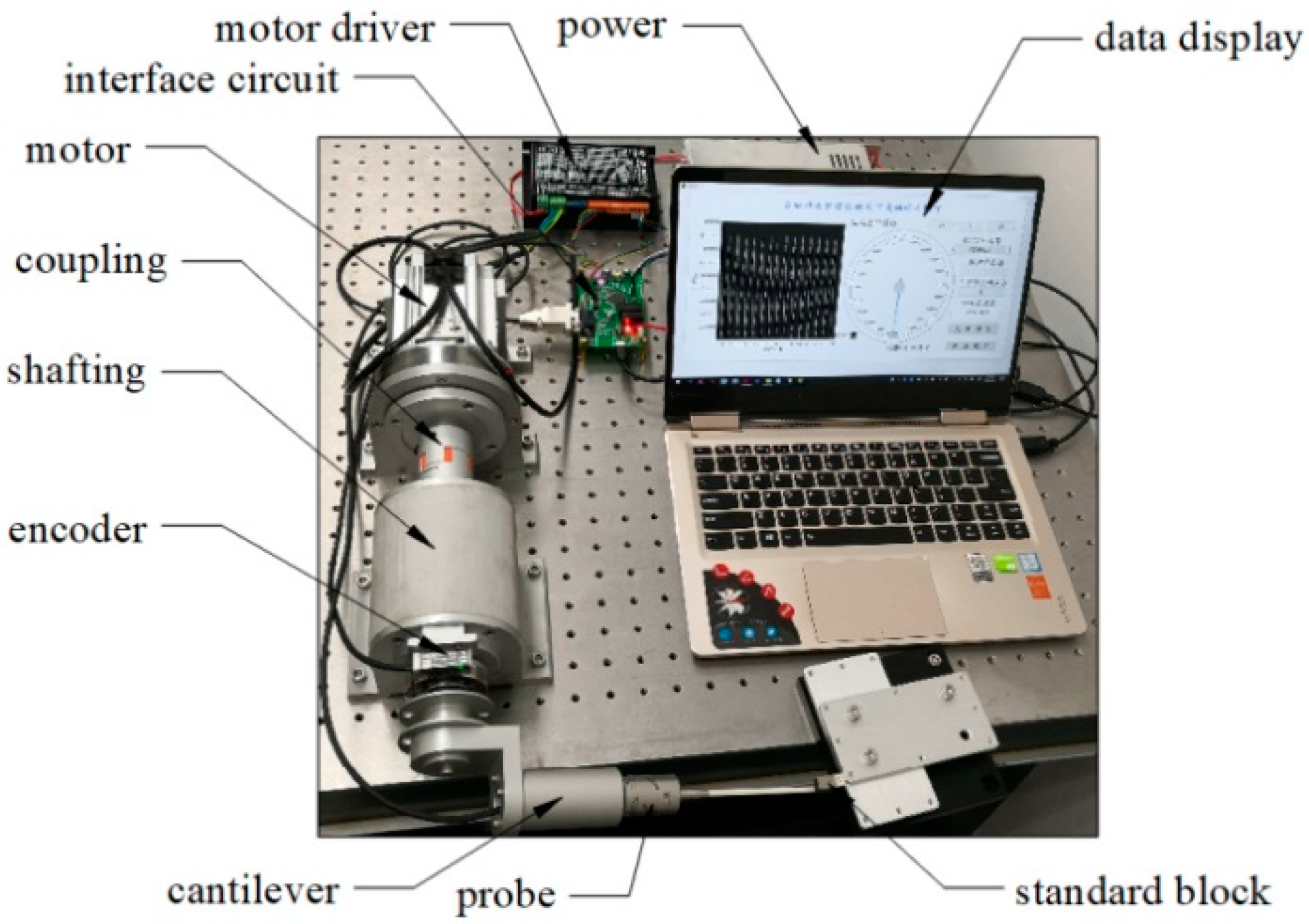
3.1. Experimental Setup

Joints are the key components for machine movement control and measurement. Therefore, it was necessary to construct a single-joint experimental setup to verify the proposed design before constructing an entire machine. This single-joint experimental setup is presented in Figure 8. The interface circuit controls the motor and drives the rotation of the shafting, cantilever, and trigger probe. The probe can touch the upper and lower sides of a standard block fixed in an optical platform. Once the probe sends a trigger signal, counting data for the encoder will be sampled and uploaded to the computer for data storage and analysis.

Figure 8. Experimental setup for a single joint [31].

3.2. Repeatability Testing

Repeatability tests with different rotational velocities were carried out using the single-joint device. Speed was controlled using pulse width modulation (PWM). After receiving the start signal, the measurement and control circuit of the joint sent the PWM signal to the motor and controlled the arm to rotate until the probe touched the surface of a measuring block and triggered angle measurement. The counter value was collected and uploaded to the computer at this time. Then, the arm was controlled to rotate reversely until the probe touched the other side of the measuring block, and the angle measurement was taken once again. The process was repeated 50 times without interruption at each duty ratio of PWM. As an example, Figure 9 presents the residual error in the count value when measuring both sides of the block with a speed of 0.67 rad/s (PWM = 6%). Table 5 lists the variance values from the repeatability experiments, where σ_U and σ_D represent the standard deviations when touching the top and bottom of the standard block, respectively.

Figure 9. Residual error in count values (speed = 0.67 rad/s).

Table 5. Variance distributions at different speeds.

PWM/Steady-State Speed (rad/s)	4%/0.23	6%/0.67	8%/1.10	10%/1.53	12%/1.97	14%/2.27
σU	0	0.85	0	1.01	1.21	0
σD	0.64	0.85	1.1	0	0	1.8

According to the experimental results, the repeatability of measurement is related to the speed of triggering. A higher triggering speed results in a poor measurement repeatability. Analysis of measurement data, it is noted that the larger the duty ratio of PWM is, the higher the probability of false trigger caused by vibration is. If the duty ratio is less than 10%, the probability of the false trigger will be greatly reduced, and the maximum standard deviation is 1.1. The pulse equivalent of incremental code signal output by the grating sensor installed on the single-joint module is 0.63″, so that the self-driven joint can reach a repeatability of 1.39″ (k = 2) when the rotational velocity is less than 1.53 rad/s.

3.3. Calibration and Measurement

To measure the length of a standard gauge block using the single joint setup, joint parameters must be calibrated. The calibration and measurement model are illustrated in Figure 10. In this figure, R is the radius of the cantilever, and r is the radius of the probe head. d₁ and d₂ represent the standard dimensions of two employed gauge blocks. θ₁ and θ₂ represent the angle values measured by the encoder when the probe touches each side of the gauge block, respectively. L₁ and L₂ are installation structural parameters for the device and α is the angle formed by L₁ and R. If only the heights of the two blocks are measured, these dimensions have the relationship shown in Equation (4). The parameters of this model can be calibrated by using standard gauge blocks of different heights.

$$\{\begin{array}{l}\cos (a)=\frac{L_1+r}{R};\\ \sin (a)=\frac{L_2}{R};\\ \cos (a+{\theta }_1)=\cos (a)\cos ({\theta }_1)-\sin (a)\sin ({\theta }_1)=\frac{L_1-d_1-r}{R};\\ \cos (a+{\theta }_2)=\cos (a)\cos ({\theta }_2)-\sin (a)\sin ({\theta }_2)=\frac{L_1-d_2-r}{R};\end{array}$$

(4)

Figure 10. Model for one-degree-of-freedom gauge block measurement.

The optimal parameters for the model can be identified through calibration. The device was used to measure a number of gauge blocks of known sizes (d₁, …, d_n) to collect multiple angle data (θ₁, …, θ_n). In this manner, the over-determined expressions in Equation (5) were obtained. The least-squares solution for this equation was solved to obtain L₁, L₂, and R.

$$\left[\begin{array}{cc}1-\cos {\theta }_1& \sin {\theta }_1\\ 1-\cos {\theta }_2& \sin {\theta }_2\\ \cdots & \cdots \\ 1-\cos {\theta }_{\mathrm{n}}& \sin {\theta }_{\mathrm{n}}\end{array}\right]\left[\begin{array}{c}{L}_1\\ L_2\end{array}\right]=\left[\begin{array}{c}r(1+\cos {\theta }_1)+d_1\\ r(1+\cos {\theta }_2)+d_2\\ \cdots \\ r(1+\cos {\theta }_{\mathrm{n}})+d_{\mathrm{n}}\end{array}\right]$$

(5)

Zero-level gauge blocks with heights of 7 mm, 7.5 mm, 8 mm, 8.5 mm, 9 mm, 9.5 mm, and 10 mm were installed. The motor rotated at a speed of 0.23 rad/s (PWM = 4%). When the probe touched the upper and lower surfaces of the gauge blocks, the encoder count values were collected, and θ_i was used to denote their difference. The experimental data are listed in Table 6. The measurement data from the 7 mm, 8 mm, 8.5 mm, 9 mm, and 10 mm blocks were used to calibrate the model parameters. The least-squares solutions are calculated L₁ = 96.5933 mm, L₂ = 248.6310 mm, and R = 266.7351 mm. After determining the optimal model parameters, the size of a measured gauge block can be calculated using Equation (6) according to the measured values.

$$d=L_1[1-\cos (\theta )]+L_2\sin (\theta )-r[1+\cos (\theta )]$$

(6)

Table 6. Experimental results for standard gauge block measurement.

Gauge Block d (mm)	10.0 ± 0.00012	9.5 ± 0.00012	9.0 ± 0.00012	8.5 ± 0.00012	8.0 ± 0.0012	7.5 ± 0.00012	7.0 ± 0.00012
Θ (rad)	0.0635957	0.0616782	0.0596319	0.0576776	0.0557386	0.0537353	0.517687

By taking the blocks with heights of 9.5 mm and 7.5 mm as components to be tested and substituting the measured values of θ_i into Equation (6), the results of 9.5148 mm and 7.4976 mm were obtained, representing measurement errors of −14.8 μm and 2.4 μm, respectively.

The results of the two experiments show that the proposed design is suitable for the self-driven AACMM. The measurement errors mainly come from the identification of structural parameters. In addition, the angle measuring error, the deformation error of the probe bar, and the gross error in the measuring process are also primary error sources.

4. Conclusions

A novel type of self-driven joint model was proposed for the design of a self-driven AACMM. The following conclusions can be drawn:

(1)

The self-driven joint model was designed. Compared with joint of AACMM, it retained the precision shaft and encoder system, and added the driving parts. Measuring points and measuring trajectories are planned, on-line automatic measurement function can be realized by the self-driven AACMM. A constant force trigger probe was installed on the self-driven AACMM to replace the hard probe and button on AACMM. Constant gaging pressure can assure uniformity of measurement results.

(2)

A virtual prototype of the self-driven AACMM designed was established and the driving moments were simulated using the MSC Adams software. A self-driven joint experimental setup was also developed. Experiments were conducted. The simulation and experimental results demonstrate that the configuration design is feasible. However, it is necessary to optimize structure and reduce weight due to its large size, which is also possible according to the simulation results presented in Figure 4.

Based on this study, the entire machine structure is being designed and optimized, control algorithms for self-driven AACMM will be studied, and it is important for us to carry out kinematic analysis and modeling of self-driven AACMM.

References

- Yu, L.D.; Zhao, H.N. Key technologies and advances of articulated coordinate measuring machines. Chin. J. Sci. Instrum. 2017, 38, 1179–1888. [Google Scholar]
- Ye, D.; Huang, Q.C.; Che, R.S. Calibration for structure parameters of multi joint CMM. J. Astronaut. Metrol. Meas. 1999, 19, 12–16. [Google Scholar]
- Kovač, I.; Frank, A. Testing and calibration of coordinate measuring arms. Precis. Eng. 2001, 25, 90–99. [Google Scholar] [CrossRef]
- Wang, P.P.; Fei, Y.T.; Lin, S.W. Calibration Technology of a Flexible Coordinate Measuring Arm. J. Xi’an Jiao Tong Univ. 2006, 40, 284–288. [Google Scholar]
- Wei, L.; Wang, C.J. Coordinate transformation and parametric calibration of multi-joint articulated coordinate measuring machine. Opto-Electron. Eng. 2007, 34, 57–61. [Google Scholar]
- Wang, X.Y.; Liu, S.G.; Zhang, G.X.; Wang, B. Calibration technology of articulated arm flexible CMM. J. Harbin Inst. Technol. 2008, 3, 1439–1442. [Google Scholar] [CrossRef]
- Santolaria, J.; Aguilar, J.J.; Yagüe, J.A.; Pastor, J. Kinematic parameter estimation technique for calibration and repeatability improvement of articulated arm coordinate measuring machines. Precis. Eng. 2008, 32, 251–268. [Google Scholar] [CrossRef]
- Cheng, W.T.; Yu, L.D.; Fei, Y.T. Kinematic model and calibration of an articulated arm coordinate measuring machine. J. Univ. Sci. Technol. China 2011, 41, 439–444. [Google Scholar]
- Gao, G.B.; Zhang, H.S.; Wu, X.; Guo, Y. Structural Parameter Identification of Articulated Arm Coordinate Measuring Machines. Math. Probl. Eng. 2016, 2016, 1–10. [Google Scholar] [CrossRef]
- Dupuis, J.; Holst, C.; Kuhlmann, H. Improving the kinematic calibration of a coordinate measuring arm using configuration analysis. Precis. Eng. 2017, 50, 171–182. [Google Scholar] [CrossRef]
- Rim, C.H.; Rim, C.M.; Kim, J.G.; Chen, G.; Pak, J.S. A calibration method of portable coordinate measuring arms by using artifacts. MᾹPAN-J. Metrol. Soc. India 2019, 34, 1–11. [Google Scholar] [CrossRef]
- Gao, G.B.; Zhao, J.; Na, J. Decoupling of Kinematic Parameter Identification for Articulated Arm Coordinate Measuring Machines. IEEE Access 2018, 6, 50433–50442. [Google Scholar] [CrossRef]
- Benciolini, B.; Vitti, A. A new quaternion based kinematic model for the operation and the identification of an articulated arm coordinate measuring machine inspired by the geodetic methodology. Mech. Mach. Theory 2017, 112, 192–204. [Google Scholar] [CrossRef]
- Zhao, H.N.; Yu, L.D.; Xia, H.J.; Li, W.S. 3D artifact for calibrating kinematic parameters of articulated arm coordinate measuring machines. Meas. Sci. Technol. 2018, 29, 065009. [Google Scholar] [CrossRef]
- Acero, R.; Brau, A.; Santolaria, J.; Pueo, M.; Cajal, C. Evaluation of the use of a laser tracker and an indexed metrology platform as gauge equipment in articulated arm coordinate measuring machine verification procedures. Procedia Eng. 2015, 132, 740–747. [Google Scholar] [CrossRef][Green Version]
- Zhao, H.N.; Yu, L.D.; Jia, H.K.; Li, W.S.; Sun, J.Q. A New Kinematic Model of Portable Articulated Coordinate Measuring Machine. Appl. Sci. 2016, 6, 181. [Google Scholar] [CrossRef]
- Pan, Z.k.; Zhu, L.Q.; Guo, Y.K. Parameter calibration for articulated arm coordinate measuring machine based on interior point algorithm. Chin. J. Sci. Instrum. 2018, 39, 117–123. [Google Scholar]
- Santolaria, J.; Yagüe, J.A.; Jiménez, R.; Aguilar, J.J. Calibration-based thermal error model for articulated arm coordinate measuring machines. Precis. Eng. 2009, 33, 476–485. [Google Scholar] [CrossRef]
- Luo, Z.; Liu, H.; Cui, X.W.; Li, D.; Tian, K. Modeling and Compensation of Thermal Deformation Error of Articulated Arm Coordinate Measuring Machine. Acta Metrol. Sin. 2019, 40, 71–77. [Google Scholar]
- Yu, L.D.; Lu, S.Y.; Zhang, W.; Zhao, H.N. Measuring system of micro-deformation of parallel double-joint coordinate measuring machine linkage. J. Electron. Meas. Instrum. 2015, 29, 1621–1629. [Google Scholar]
- Vrhovec, M.; Kovač, I.; Munih, M. Measurement and compensation of deformations in coordinate measurement arm. In Proceedings of the IEEE International Symposium on Optomechatronic Technologies, Toronto, ON, Canada, 25–27 October 2010. [Google Scholar]
- Luo, Z.; Liu, H.; Li, D.; Tian, K. Analysis and compensation of equivalent diameter error of articulated arm coordinate measuring machine. Meas. Control 2018, 51, 16–26. [Google Scholar] [CrossRef]
- Gąska, A.; Gąska, P.; Gruza, M. Simulation Model for Correction and Modeling of Probe Head Errors in Five-Axis Coordinate Systems. Appl. Sci. 2016, 6, 144. [Google Scholar] [CrossRef]
- Sładek, J.; Ostowska, K.; Gąska, A. Modeling and identification of errors of coordinate measuring arms with the use of a metrological model. Measurement 2013, 46, 667–679. [Google Scholar] [CrossRef]
- Ostrowska, K.; Gąska, A.; Kupiec, R.; Gromczak, K.; Wojakowski, P.; Sładek, J. Comparison of accuracy of virtual articulated arm coordinate measuring machine based on different metrological models. Measurement 2019, 133, 262–270. [Google Scholar] [CrossRef]
- Zheng, D.T.; Du, C.T.; Hu, Y.G. Research on optimal measurement area of flexible coordinate measuring machines. Measurement 2012, 45, 250–254. [Google Scholar] [CrossRef]
- Hu, Y.; Jiang, C.; Huang, W.; Hu, P.H. Optimal measurement area of articulated coordinate measuring machine calculated by ant colony algorithm. Opt. Precis. Eng. 2017, 25, 1486–1493. [Google Scholar] [CrossRef]
- González-Madruga, D.; Barreiro, J.; Cuesta, E.; González, B.; Martínez-Pellitero, S. AACMM performance test: Influence of human factor and geometric features. Procedia Eng. 2014, 69, 442–448. [Google Scholar] [CrossRef]
- Cuesta, E.; Mantaras, D.A.; Luque, P.; Alvarez, B.J.; Muina, D. Dynamic deformations in coordinate measuring arms using virtual simulation. Int. J. Simul. Model. 2015, 14, 609–620. [Google Scholar] [CrossRef]
- Eduardo, C.; Alejandro, T.; Hector, P.; González-Madruga, D.; Martínez-Pellitero, S. Sensor prototype to evaluate the contact force in measuring with coordinate measuring arms. Sensors 2015, 15, 13242–13257. [Google Scholar]
- Hu, Y.; Huang, W.; Hu, P.H.; Yang, H.T. Design of modular articulation in self-driven AACMM. Opt. Precis. Eng. 2018, 26, 2021–2029. [Google Scholar] [CrossRef]
- Siciliano, B.; Sciavicco, L.; Villani, L.; Oriolo, G. Robotics: Modelling, Planning and Control; Xi’An Jiaotong University Press: Xian, China, 2015. [Google Scholar]
- Li, Z.G. Introduction and Instances of ADAMS, 2nd ed.; National Defense Industry Press: Beijing, China, 2014. [Google Scholar]
© 2019 by the authors. Licensee MDPI, Basel, Switzerland. This article is an open access article distributed under the terms and conditions of the Creative Commons Attribution (CC BY) license (http://creativecommons.org/licenses/by/4.0/).