A Study on Development of the Camera-Based Blind Spot Detection System Using the Deep Learning Methodology

Abstract

One of the recent news headlines is that a pedestrian was killed by an autonomous vehicle because safety features in this vehicle did not detect an object on a road correctly. Due to this accident, some global automobile companies announced plans to postpone development of an autonomous vehicle. Furthermore, there is no doubt about the importance of safety features for autonomous vehicles. For this reason, our research goal is the development of a very safe and lightweight camera-based blind spot detection system, which can be applied to future autonomous vehicles. The blind spot detection system was implemented in open source software. Approximately 2000 vehicle images and 9000 non-vehicle images were adopted for training the Fully Connected Network (FCN) model. Other data processing concepts such as the Histogram of Oriented Gradients (HOG), heat map, and thresholding were also employed. We achieved 99.43% training accuracy and 98.99% testing accuracy of the FCN model, respectively. Source codes with respect to all the methodologies were then deployed to an off-the-shelf embedded board for actual testing on a road. Actual testing was conducted with consideration of various factors, and we confirmed 93.75% average detection accuracy with three false positives.

1. Introduction

Various global automobile companies are actively conducting research on development of an autonomous vehicle. The autonomous vehicle, known as the self-driving vehicle, is a vehicle which can perceive an environment and navigate without human intervention [1]. According to the Society of Automotive Engineers (SAE), the technology of the autonomous vehicle is categorized into six levels, and most global automobile companies have a plan to release a fully autonomous vehicle by 2020 [2]. Those six levels are summarized in

Table 1. Six levels of the autonomous driving technology.

Levels	Description
Level 0 No Automation	The driver fully takes responsibility to operate the vehicle.
Level 1 Driver Assistance	The driver operates the vehicle with some driving assistance features included in the vehicle.
Level 2 Partial Automation	Automated features such as auto-steering, auto-acceleration, etc. need to be installed in the vehicle, and the driver needs to engage in driving the vehicle and monitoring the environment.
Level 3 Conditional Automation	The driver is not required to monitor the environment but needs to control the vehicle when necessary.
Level 4 High Automation	The driver is required to optionally control the vehicle, and all the driving functions in the vehicle are operated under certain conditions.
Level 5 Full Automation	The driver is required to optionally control the vehicle, and all the driving functions in the vehicle are operated under all conditions.

[3].

One of the well-known electric automobile companies in the USA has the most advanced autonomous vehicle technology in the current market. Vehicles in this company have numerous driving assistant features such as autopilot, summon, etc. [4]. Moreover, the autonomous vehicle division of the most famous IT company located in Mountain View, USA, has conducted testing of the fully self-driving vehicle in Arizona, USA since October 2017 [2].

However, the most important technical aspect to achieve fully autonomous driving is safety. According to the accident report published in May 2016, a driver who operated an electric vehicle was killed due to a collision with a semi-trailer on a highway in Florida, USA [3]. The main reason for this crash was that the vehicle was driven by the autopilot feature consisting of three systems: auto-steer, Auto Lane Change System (ALCS), and Traffic-Aware Cruise Control (TACC), but the driver heavily depended upon vehicle automation technologies which belong to level 2 in Table 1. One interesting point from the accident report is that the level 2 technology does not show high system reliability. This limitation of the vehicle automation technologies injects motivation into this research. Especially, this research focused on the safety feature related to blind spot detection.

Blind spot detection is a core technology in terms of the ALCS, as mentioned above. In addition, 4–10% of all traffic crashes refer to side-swipe accidents caused by blind spot detection [5]. For this reason, giving an audio-visual warning to drivers is necessary when misdetection of the blind spot occurs. Therefore, this study proposed development of the camera-based blind spot detection system using a deep learning methodology.

This paper is organized as follows: Section 2 describes the technological aspects of the blind spot detection system and provides a brief literature review. Section 3 presents methodologies and a research framework for system development. Experimental results with pre-recorded video images and live video images on a real road are discussed in Section 4 and Section 5, respectively. Section 6 describes conclusions, research limitations, and future work.

2. Related Work

There are two types of blind spot detection systems. The first type is radar sensors developed by Robert Bosch GmbH, Germany, as shown in Figure 1 [6,7].

Electromagnetic wave-based two radar sensors are mounted in the rear bumper, and each sensor measures a distance between a radar-equipped vehicle and an approaching vehicle [8]. This type of the system gives visual alarm to the driver when the approaching vehicle is either very close to the radar-equipped vehicle or in the blind spot. This system also gives audio alarm to the driver when the radar-equipped vehicle changes a lane while the approaching vehicle is in the blind spot [8]. The main issue of this system is that it does not detect very fast approaching vehicles and motorcycles well [8].

The second type is the camera-based blind spot detection system. One of the Japanese automobile companies introduced this system in 2013. One camera is mounted underneath the side mirror on the passenger side. This camera is activated when the right turn signal is on or a driver pushes the button on the turn signal switch [9]. Figure 2 shows how this system works.

However, this camera-based system also has several issues: (i) the system provides a guideline to see a distance between the system-equipped vehicle and target vehicle in the next lane through the screen, but it does not give any visual or audible warning to drivers, unlike the radar-based blind spot system; and (ii) the mounted camera is very vulnerable to rainwater and contaminants. For this reason, many studies have been conducted to provide the reliable camera-based blind spot detection system.

The work in [10] proposed a vision-based blind spot detection system based on optical flow techniques. This system is composed of four computational steps: (i) image processing; (ii) pixel-wise clustering; (iii) analysis of clusters; and (iv) pattern recognition. The image processing step is associated with separating relevant features from the environment due to the expectation of reducing computational time. In this step, the Canny edge extractor is applied to the original incoming image and pixels with a positive value are used for calculating optical flow. In the pixel-wise clustering pixel, Canny edge pixels are grouped together to detect the clusters of pixels. Each cluster of pixels is a candidate for vehicle objects in the processed image. To determine groups of pixels and their likelihood to form a single object, classical clustering techniques are used. Note that this step is the first sub-step in the clustering stage, and the second sub-step is to group or merge two or more clusters into a single cluster based on distance criteria. The reason for splitting this step into two sub-stages is due to the possibility that two objects could be positioned close together. In the analysis of clusters stage, the selected clusters are used as a seed point to find the frontal part of a vehicle through the double-stage detection algorithm consisting of a pre-detector, pre-warning, etc. Once vehicle candidates are located, they are classified by the Support Vector Machine (SVM) in the pattern recognition stage. This research reported that the detection accuracy of testing the system was 99% with five false positive detections.

The work in [11] proposed a motion-based blind spot detection system based on the optical flow calculation as well. A template matching technique was initially considered to detect and track a vehicle, but this research reported poor performance of the template matching technique due to a difficulty to capture a motion and shape of the vehicle. The proposed algorithm is composed of several steps: (i) specify a blind spot zone in the grayscale image; (ii) extract features; (iii) estimate the motion vector through calculation of the optical flow; (iv) label valid features as potential features; (v) eliminate noise and finally; and (vi) label vehicle features. The experimental result shows that vehicles were successfully detected and tracked in thirty-eight situations out of forty-one situations without any false positive alarms.

The authors of [12] proposed a blind spot monitoring system using the Histogram of Oriented Gradients (HOG) descriptor and SVM. The proposed algorithm introduces four main steps. Once an image frame is captured by a single rear-view camera, the first step is to set the detection window for vehicle detection in either the left or right blind spot area. The second step is to detect vehicles in the detection window using the HOG descriptor and SVM. The authors claimed that the HOG descriptor and SVM showed outstanding performance and reliability. The third step is to estimate the moving direction of the detected vehicles from the previous step. The last step is to generate an alarm signal if vehicles are in the blind spot area. Furthermore, a high-speed algorithm consisting of two additional concepts, i.e., selective filtering of the HOG features and fast estimation of moving direction, is introduced for real-time evaluation with an embedded system. The authors evaluated the developed algorithm with consideration of various environments and vehicles, and measured performance evaluation using recall and precision. The evaluation of the basic algorithm on both urban areas and highways resulted in 98.62% precision and 99.82% recall, respectively. When evaluating the high-speed algorithm, the authors reported 97.26% precision and 99.65% recall, respectively.

In [13], the camera-based blind spot detection system in conjunction with a network based on AlexNet was proposed as a real-time embedded system application. In this network structure, there are four blocks after the first convolutional layer, and each block is designed by various combinations of the concepts based on the Visual Geometry Group (VGG), depthwise separable convolutions, residual learning, and the squeeze-and-excitation module. For this reason, four different neural networks are established: (i) only VGG blocks-based network; (ii) network with a combination of depthwise separable convolution and residual learning (Sep-Res); (iii) network with a combination of depthwise separable convolution and the squeeze-and-excitation module (Sep-SE); and (iv) a combination of all three parts (Sep-Res-SE). Two datasets were employed to evaluate each network, and the authors reported that the VGG blocks-based network showed slightly higher test accuracy than other networks, but the Sep-Res-SE network showed better performance in terms of overall evaluation including inference speed and memory cost. Note that the Sep-Res-SE network showed 97.58% detection accuracy.

According to the literature research above, there are no doubts that the camera-based blind spot detection system has a potential possibility to be improved. However, some studies concentrate on proposing algorithms and techniques in conjunction with the methodologies of image processing and classification to detect moving vehicles in the blind spot. Besides, to the best of our knowledge, studies about blind spot detection using a Fully-Connected Network (FCN) only have not been reported. This point corresponds with the research objective, i.e. developing a camera-based blind spot detection system using the deep learning methodology. In other words, our main goal was to develop lightweight software that can be installed on an embedded board that has limited hardware specifications by employing the FCN, HOG descriptor, sliding window technique, heat map, and thresholding. Those concepts are further discussed in Section 3.

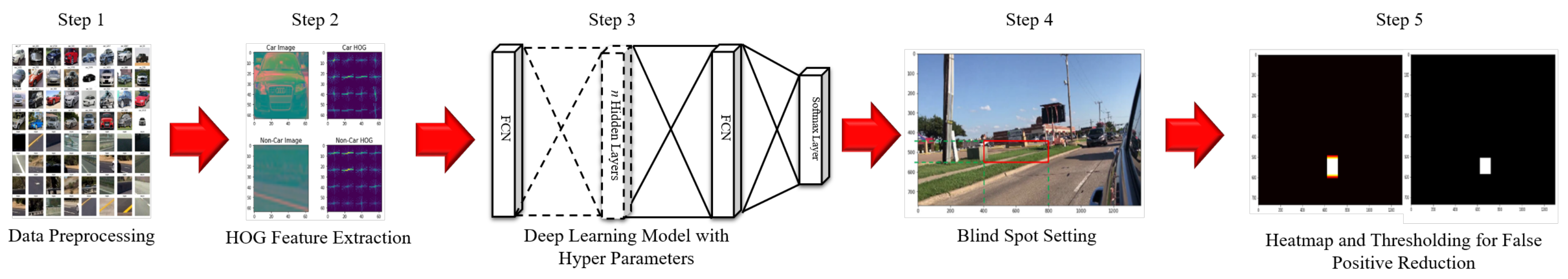
3. Methodologies and Research Framework

3.1. Dataset Preprocessing

The first step in the research framework is to secure an image dataset for training a model. The best case scenario was to take a picture of every single vehicle by ourselves, but it was infeasible due to the time constraint. Hence, we decided to use datasets for vehicles and non-vehicle objects from [14,15,16], and a total of 8144 vehicle images were extracted. Figure 3 shows the examples of vehicle images.

In the beginning of the project life cycle, all 8144 vehicle images were planned to be used for training, but there are several issues with respect to those images: (i) vehicle images have various angles; (ii) some images contain a banner and other vehicles in the background; and (iii) there is a difference in terms of image quality. Each issue was solved as follows:

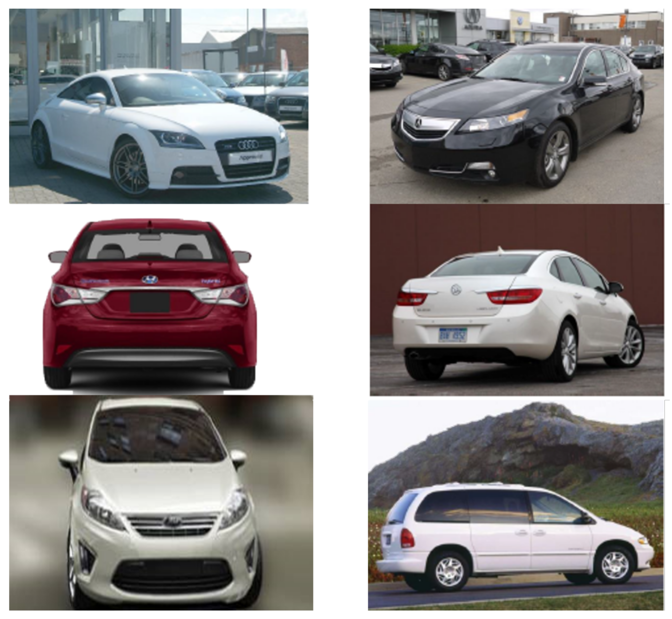
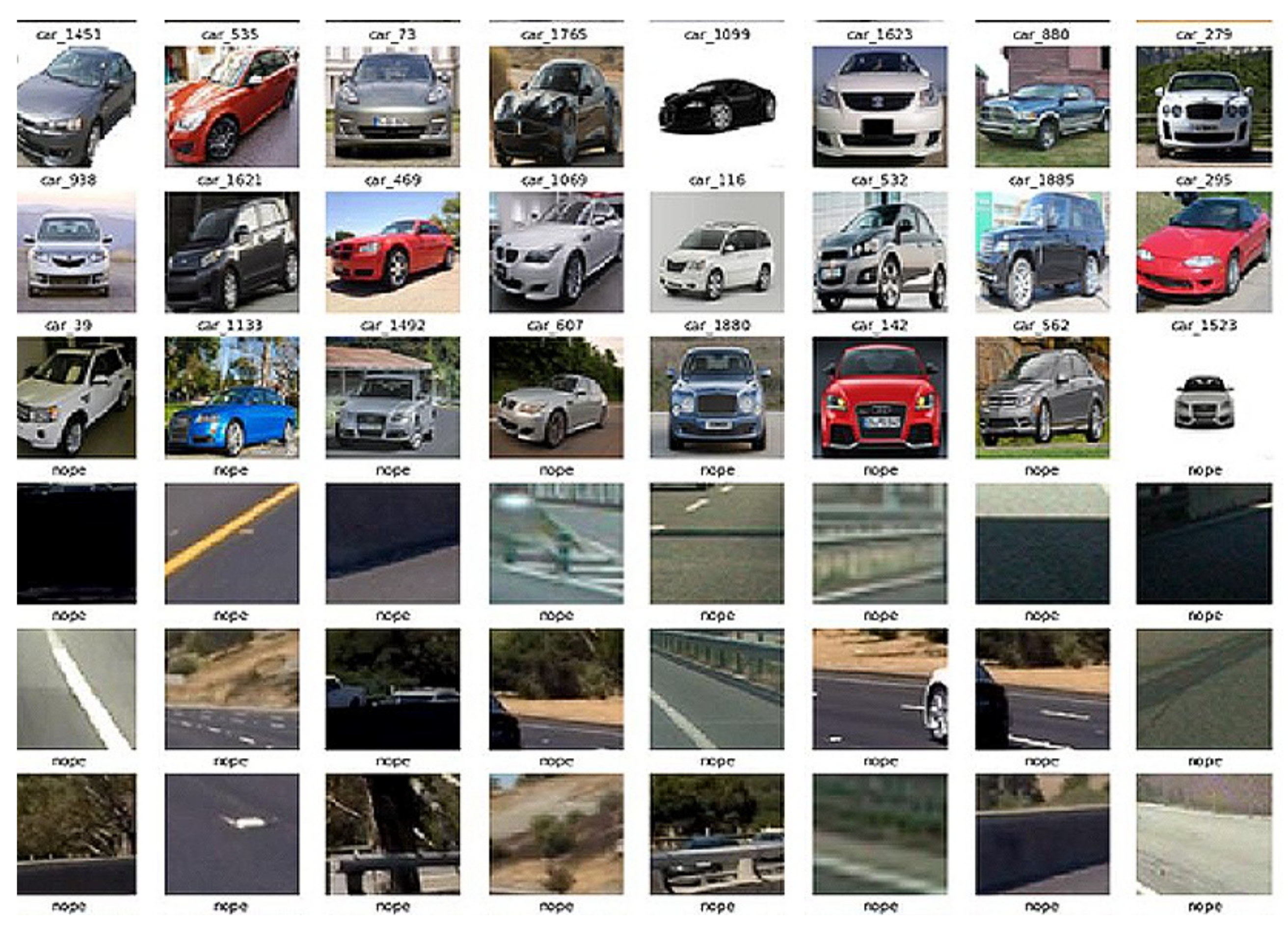
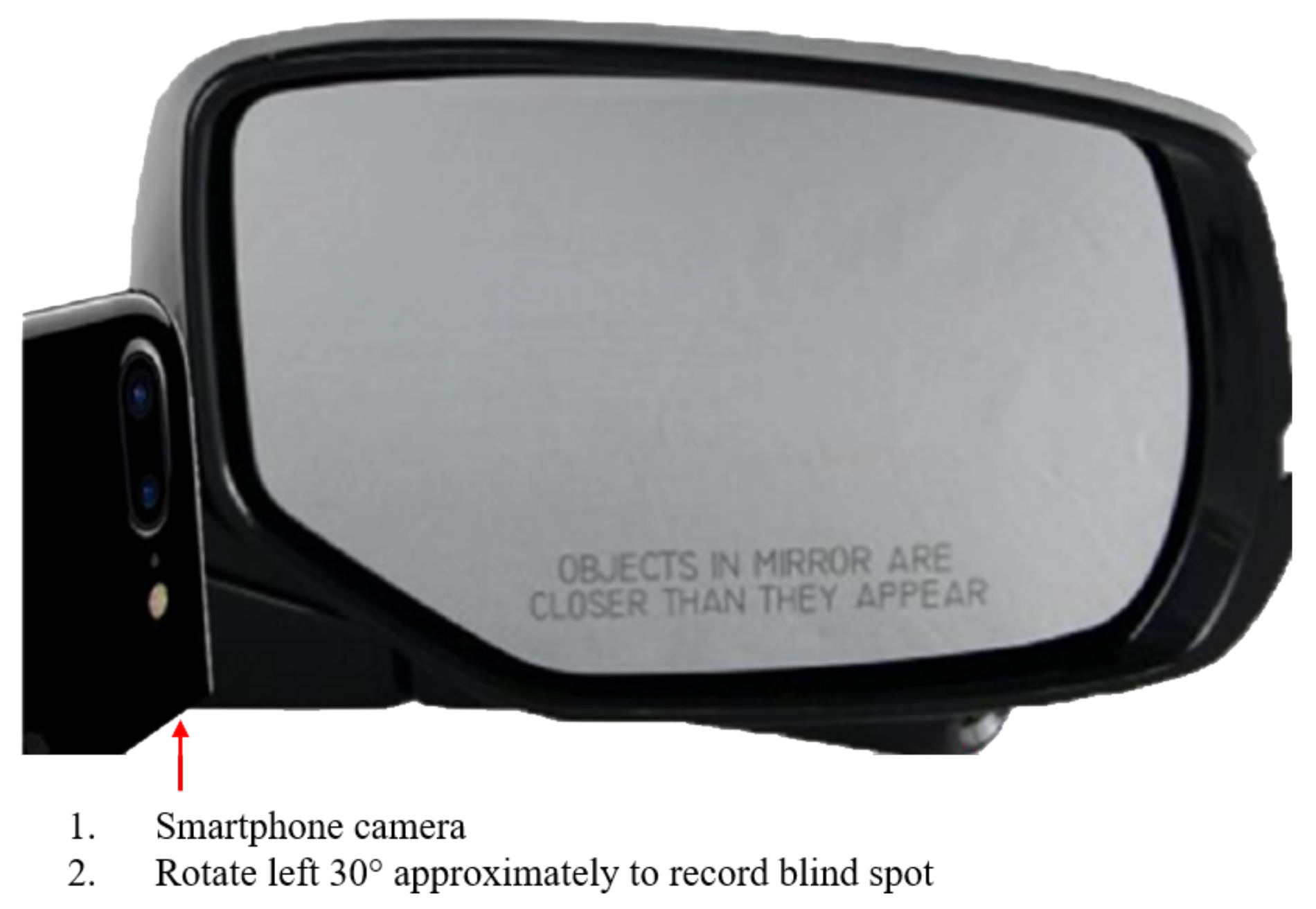
• Preliminary testing was conducted using the video recorded by the smartphone camera shown in Figure 4 prior to actual testing on a real road. For this reason, only vehicle images with front and front-left angles were extracted due to the viewing angles of the blind spot shown in Figure 5, and a total of 2000 images out of 8144 images were selected.
• After the banner and other vehicles in the background were removed, the background was filled in with white.
• All selected images were edited by the sharpen function to have outstanding image quality.

As mentioned above, approximately 9000 non-vehicle images were also extracted and used for training a model. Figure 6 shows data visualization of the vehicle and non-vehicle images.

3.2. Data Reduction and Representation Learning

Data reduction refers to reducing high-dimensional data into low-dimensional data to deal with several issues such as the curse of dimensionality and selection of optimal boundary [17]. Furthermore, data reduction is required due to both practical and theoretical reasons, e.g., removal of irrelevant features, the perspective of computation and machine learning, the perspective of probability and statistics, etc. [18]. Dimension reduction can be implemented by a variety of strategies for diverse applications. In [19], three well-known data reduction strategies, namely dimensionality reduction, clustering, and sampling, were discussed. Dimensionality reduction is related to reducing the number of random variables, and feature selection and feature extraction are the representative methodologies of dimensionality reduction. Clustering groups objects into similar groups, and sampling is used to determine if a small set of samples represents the entire dataset [19]. Among the described methodologies of data reduction above, we picked feature extraction belonging to dimensionality reduction at our discretion. Feature extraction in conjunction with the HOG descriptor is further discussed in Section 3.3.

We also examined several studies to see which dimensionality reduction methodologies were used in which areas. In [20,21], Principal Component Analysis (PCA) was employed to reduce data dimensions. Note that PCA is one of the state of the art techniques to reduce an unlabeled high-dimensional input dataset for the purpose of feature extraction. However, the authors of [20,21,22], interestingly, adopted the Restricted Boltzmann Machine (RBM) model for representation learning, also known as feature learning. The reason Deep Neural Networks (DNNs) need to be used for representation learning is that they contain their own way of expressing data, which converts input data into a numerical form that is easy to recognize. Especially, DNNs can learn from data by parameterizing data representation methods [23]. However, we decided not to adopt one of the DNN models for representation learning because it would be too much to run two or more deep learning models on limited hardware specifications.

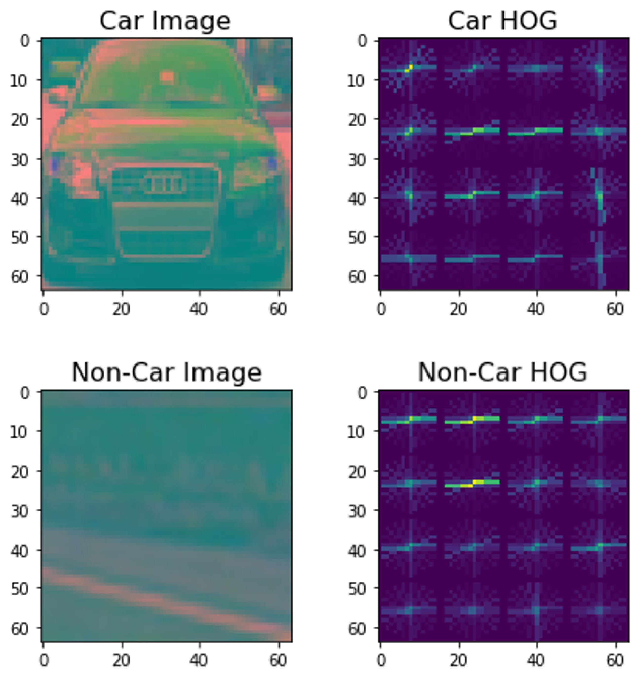
3.3. Histogram of Oriented Gradients (HOG)

One of the popular methodologies for feature extraction is the HOG descriptor, and this is very powerful for objects detection, especially human detection. The reason for employing the HOG descriptor is that this methodology can also be used in tasks related to autonomous vehicles [24]. This methodology is composed of five stages [25]: (i) normalize images; (ii) compute gradients in X (horizontal) and Y (vertical); (iii) compute gradients histograms; (iv) normalize blocks; and (v) collect HOG descriptors from overlapping blocks and cover into a feature vector.

The first stage, image normalization, is required to provide better illumination invariance such as lighting, shadows, etc. by normalizing cells in the block. Note that the definition of the cells and blocks is that once an image window is divided into small or large spatial regions, these are called cells, which consist of multiple pixels and can be rectangular or circular, and blocks, which incorporate multiple cells, respectively. However, image normalization was not applied in this research because it does not make a big impact on performance [25]. The second stage focuses on computing image gradients in X and Y. This stage can be performed by capturing the image edge or structure based on the locally dominant color channel. By doing so, it is also possible to provide better resistance to illumination variations. The third stage is about computing gradients histograms by collecting the information of gradient orientation locally. As mentioned in the first step above, computing gradients histogram is based on the concept of cells; that is, a local 1D histogram of gradient or edge orientations over the pixels in the cell is accumulated for each cell, and the combined histogram forms the representation of the orientation histogram [25]. After that, the range of a gradient angle is divided into a fixed of bins. The fourth stage is to compute normalization by accumulating a measure of local histogram “energy” over blocks. Note that this refers to normalized cells in the block because each cell is shared by multiple blocks. For this reason, a cell with different normalizations possibly appears in a final output vector. The last stage is to collect HOG descriptors over the detection window, which refers to the normalized block descriptors in the previous stage. The detailed concept of the HOG descriptor is available in [25].

The main objective of data preprocessing and feature extraction through the HOG descriptor is to make the input dataset for a deep learning model. Before applying the HOG descriptor, a size of all the images is fixed at 60 px × 60 px because every image has a different size. Eleven orientations, sixteen pixels per cell, and two cells per block were used for feature extraction, thus the total length of the feature vector was 1188. Thus, there were 1188 pixels in a single image, which means that 3600 pixels were converted into 1188 HOG features for both vehicle and non-vehicle objects. Figure 7 shows an example of feature extraction through the HOG descriptor.

3.4. Deep Neural Networks and Fully Connected Network

Before discussing our chosen deep learning model, we examined a variety of DNNs. The first DNN model we examined is a FCN, which is the simplest DNN model. The reason for calling it the simplest DNN model is that the DNN can be implemented by solely fully-connected layers [26]. All the output activations in fully-connected layers consist of a weighted sum of all the input activations, thus all the outputs are connected to all the inputs [26]. However, the well-known disadvantage of this model is that it requires a large amount of storage and computation, but this issue could be solved by removing some connections between the activations [26].

In [27], the authors proposed deep Convolutional Neural Networks (CNNs), which are composed of five convolutional layers followed by max pooling layers and three fully-connected layers with a final 1000-way softmax. Besides, Rectified Linear Units (ReLus) were applied to the output of every convolutional and fully-connected layer. One interesting point in this research was that two GPUs were employed to train the proposed model due to the size of the adopted dataset. By doing so, the authors mentioned that it was possible to reduce error rates and achieve less training time than when using a single GPU. Note that other concepts such as local response normalization, two forms of data augmentation and dropout to avoid an overfitting issue, etc. were employed.

The study, which began with a strong motivation that the deeper the network, the better the accuracy, discussed the deep residual learning methodology, also known as the ResNet [28]. In this research, however, the authors pointed out a degradation problem caused by vanishing or exploding gradient if a network gets deeper. To avoid such a problem, the authors inserted shortcut connections into the plain network to turn the network into its counterpart residual version. Two advantages were claimed: (i) easy to optimize; and (ii) gain accuracy from considerably increased depth, but the disadvantage of residual networks is that the computational and memory costs could be linearly increased to improve performance [29].

In [30], the authors proposed a deep learning model that combines two Recurrent Neural Networks (RNNs) consisting of an encoder and a decoder. This model is also called Sequence to Sequence (Seq2Seq). The encoder basically creates a fixed size context vector from the input sequence of the model, and the decoder uses this context vector as an input to create a translated output sequence. The Seq2Seq model is very effective in generating responses, but the dialogue response generated by the Seq2Seq model tends to be less diverse [31].

The authors of [32] proposed the abstractive text summarization method based on Generative Adversarial Networks (GANs) consisting of the generator and discriminator. In this research, the authors pointed out that GAN is very powerful in terms of computer vision and image generation areas, but it is challenging to generate discrete outputs.

As described above, DNNs can be organized into different forms depending on how they are applied: (i) the FCN is suitable when all the input data have to be jointly considered; (ii) the CNN is optimized to extract spatial features; and (iii) the RNN is appropriate for sequential data such as natural language [33]. Back to a discussion of our chosen deep learning model, the basic idea in this research is a simple neural network based on the following equation:

$$H\left(x\right)=Wx+b$$

(1)

where H(x) is a hypothesis, x indicates input data variables or data, and W and b denote weights and bias, respectively. This equation refers to neural network learning as a linear regression model, and the main objective is to find a set of the optimized network parameters by minimizing a cost function [34]. One of the basic cost functions for this neural network is the gradient decent algorithm which always converges to the global minimum [34]. The main limitation is that, although it is optimized for linear regression, it has a difficulty to linearly separate an exclusive OR (XOR) gate [35]. However, this limitation could be solved by the concept of backpropagation [36,37], and this algorithm became the origin of a DNN. A DNN in this research refers to the number of layers in the network that is derived from a simple neural network; in other words, the more layers between the input and the output layers, the deeper the network [38]. The basic DNN architecture is the FCN consisting of an input layer, output layer, and a hidden layer. There are two things to keep in mind to use this model, i.e. preventing the issues of vanishing gradient and overfitting. For this reason, finding and setting the best parameters is very important. Parameters here refer to the number of inputs, hidden layers, learning rate, epoch, etc.

For our research, we decided to employ the FCN model with Adam optimizer and ReLus activation instead of gradient descent for improving training accuracy. The main computational advantage of our model based on HOG and FCN is that both HOG and FCN are simple matrix calculation-based, thus they are easily paralleled, and the GPU-based embedded toolkit with limited specifications and computations is easy to use. All the detailed mathematical concepts related to the employed FCN model are described as follows:

• Input: X ∈${\mathbb{R}}^{m\times \mathrm{1,188}}$
• Output: Y ∈${\left[0,1\right]}^{m\times 2}$
• FCN

   -

  ReLu activation function: ${\mathsf{\Omega }}_i=max(0,W_{i}x+h_i)$

   -

  Y = $\mathsf{\Theta }\left({\mathsf{\Omega }}_1(\dots {\mathsf{\Omega }}_i\left(X\right))\right)$

• Softmax output layer: $\mathsf{\Theta }\left({\mathsf{\Omega }}_i^j\right)=\frac{e^{X_j}}{{\sum }_{k=1}^K{e}^{X_k}}$, where i = 1, …, 3 and is defined as the number of layers, and j = 1, …, K and is defined as output classes
• Categorical cross-entropy objective function: $\mathcal{H}(Y,Y^{\prime })=-{\sum }_m{Y}_{m}log\left(Y_m^{\prime }\right)$, where m is the batch size, Y is an actual output, and Y’ is a predicted output
• Empirical loss function: $\mathcal{L}=\frac{1}{m}\mathcal{H}(Y,Y^{\prime })$

Our goal was to achieve more than 95% training and testing accuracy with the FCN model. If this goal could not be achieved by the FCN model, Plan B was to employ any of the deep learning models such as CNNs, RNNs, etc. To see whether the FCN model achieved more than 95% accuracy, we started to train the model, which was implemented by open source software on the cloud platform. Hardware specifications for training the model are as follows:

• Machine Name: n1-standard-4
• Virtual CPUs: 4
• Memory: 15 GB
• Hard Disk Drive = 200 GB

In addition, the model was trained with hyperparameters as follows:

• the number of inputs (features): 1188 images
• the number of hidden layers: 2
• the number of units in hidden layers: 1188 in the first hidden layer and 594 in the second hidden layer
• learning rate = 1 × 10${}^{-6}$
• epoch = 10

According to training and testing results shown in

Table 2. Experimental results of model training and testing.

Epoch	Training Loss	Training Accuracy	Testing Loss	Testing Accuracy
1	0.5111	78.8%	0.2019	87.8%
2	0.1750	93.4%	0.1337	95.6%
3	0.1254	96.3%	0.1014	96.9%
4	0.0982	97.3%	0.0817	97.4%
5	0.0782	98.1%	0.0692	97.8%
6	0.0636	98.5%	0.0593	98.1%
7	0.0527	98.9%	0.0522	98.3%
8	0.0448	99.1%	0.0498	98.5%
9	0.0379	99.3%	0.0443	98.8%
10	0.0321	99.4%	0.0389	99.0%

, the FCN model was employed for further steps as the training and testing accuracies achieved were 99.4% and 99.0%, respectively.

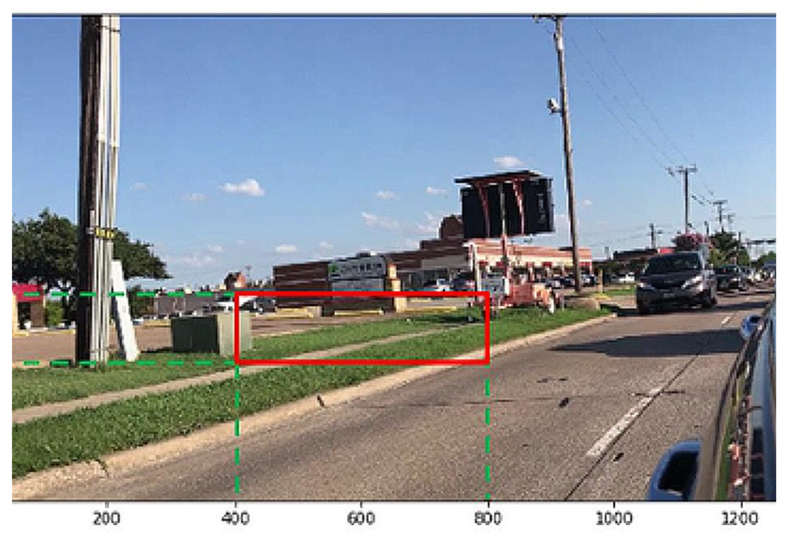
3.5. Blind Spot Setting for Vehicle Detection

The main methodology to detect a vehicle in a blind spot is that, once a vehicle enters a blind spot, which is defined based on x and y axes, a blue rectangle box detects a vehicle using the sliding window technique. The size of the video image, which was recorded using the set up in Figure 4, is approximately 1300 px × 800 px. In this video image, we manually and visually checked that a blind spot has a range of 400–800 px in x-axis and 450–550 px in y-axis, as shown in Figure 8.

One thing to keep in mind is that this system is not intended for object classification; that is, this system does not intend to identify whether the detected object is a vehicle or not. For this reason, a rectangle box focuses on detecting vehicle features; for instance, once the front view of a vehicle enters a blind spot, a license plate, radiator grill, headlights, etc. can be possibly detected by a rectangle box. In the case of a side view of a vehicle, a tire, alloy wheel, side mirror, etc. can be detected. Therefore, once any of the vehicle features is detected in a blind spot, a rectangle box is displayed on the screen. However, the size of the rectangle box, also known as rectangle threshold, is associated with false positive reduction, and this point is discussed in the next section.

3.6. False Positive Reduction

One of the main potential issues is false positive detection. This means that, even though the object is not a vehicle, the system detects it either in or out of a blind spot through the sliding window technique. To minimize this issue, two concepts, namely heat map and thresholding, are used. The fundamental concept of the heat map is to visualize an image by representing each pixel by the color corresponding to its magnitude [39,40]. Assume that an image, $x=\left\{x_p\right\}$, and a classification function, $f\left(x\right)$, are given where p denotes a pixel. Here, the function, $f\left(x\right)$, is used for indicating the presence of an object in the image and can be learned very well by a deep neural network [40].

Based on this, the heat map is denoted as:

$$h=\left\{h_p\right\}=\mathcal{H}(x,f,p)$$

(2)

where $\mathcal{H}$ is a function derived from a class discriminant f. Note that a value is assigned to each pixel, p, by $\mathcal{H}$. In addition, h is visualized as an image since its dimensionality is same as x [40].

Thresholding refers to the technique of image segmentation, and it is denoted as:

$$T=T[x,y,p(x,y),f(x,y\left)\right]$$

(3)

where T is the threshold value, x and y are the coordinates of the threshold value, $p(x,y)$ is points in gray-level image pixels, and $f(x,y)$ is gray-level image pixels [41,42]. There are two main thresholding techniques: global and local. The major difference is that global thresholding applies one threshold value to the whole image, while local thresholding applies different threshold values to different areas of the image [41]. Among these two techniques, the simpler one is global thresholding, which was adopted in this research, and denoted as:

$$g(x,y)=\left\{\begin{array}{cc}0\hfill & iff(x,y)\le T\hfill \\ 1\hfill & iff(x,y)>T\hfill \end{array}\right.$$

(4)

where T is the threshold value, and $g(x,y)$ = 0 or 1 means an object and background, respectively [41,42]. Note that $f(x,y)$ is replaced with the heat map, $h_p$, and we initially set 10 to the value of thresholding, T. The main objective of both concepts is to maximize a probability that the detected (target) object is a vehicle.

As mentioned in the previous section, the size of a rectangle box is also used for false positive reduction. Assume that vehicles are seen in a blind spot, but they are far away from a blind spot. In this case, vehicles are seen smaller than presenting in a blind spot. The system recognizes them as vehicles but does not need to detect them. For this reason, if a rectangle box given by the heat map is smaller than a particular value, the system rejects it and the false positives can be reduced.

According to all the methodologies described above, the entire research framework is depicted in Figure 9.

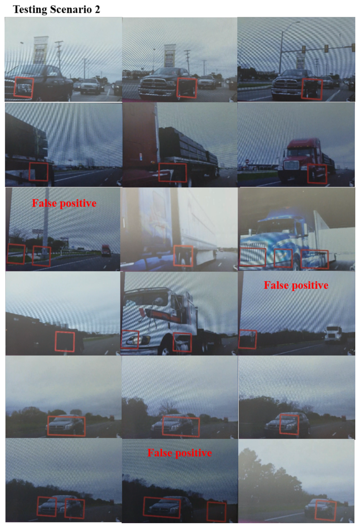
4. Experiments with Record Video Images

Prior to conducting experiments, we came up with two possible scenarios. The first scenario is when the system-equipped vehicle stops or moves more slowly than a target vehicle. The second scenario is when the system-equipped vehicle moves more quickly than a target vehicle. Based on these, the research framework was applied to two video images recorded using the set up in Figure 4. Four vehicles and two vehicles entered a blind spot in the first and second scenarios, respectively. As mentioned above, the research framework was implemented in open source software on the cloud platform. Overall, 28.89 s were taken to extract HOG features, and 461 frames were captured in the first scenario. In addition, in total, 386 frames were captured in the second scenario. In the first experiments with the first scenario, we encountered false positive issues. Here, the meaning of false positive is that, despite the object not being associated with a vehicle, it was captured as a vehicle feature. Most false positive issues were caused by a vehicle shadow. To solve such issues, we analyzed the whole source code again for the purpose of root cause analysis and realized that the causes resulted from hyperparameters. Note that hyperparameters this time refer to the size of a rectangle box, threshold value, and memory size, and these are different from the hyperparameters of the deep learning model, as mentioned in Section 3.4. The identified solution with respect to the size of a rectangle box was that, once it was increased, false positives were reduced. For this reason, the size of a rectangle box was maximized to 9000. As described above, the initial threshold value was 10. This value was reduced to 2, but the problem was that, while performance was improved, false positives were increased. Hence, the threshold value did not change for testing on the cloud platform. The concept of detection memory is that it is used to remember which pixels presented vehicles in previous frames. Since the system detects a vehicle based on vehicle features, detection memory helps the system remember a vehicle in a blind spot. Hyperparameters were tuned several times, and the best combinations used for a proof of concept on the cloud platform were as follows:

• the size of a rectangle box: 9000
• the threshold value: 10
• the size of detection memory: 4

Figure 10 depicts experimental results of each scenario, and we confirmed that vehicles in the recorded video images were correctly detected without false positives. Note that the vehicle license plate and driver face were shaded in gray for privacy reasons.

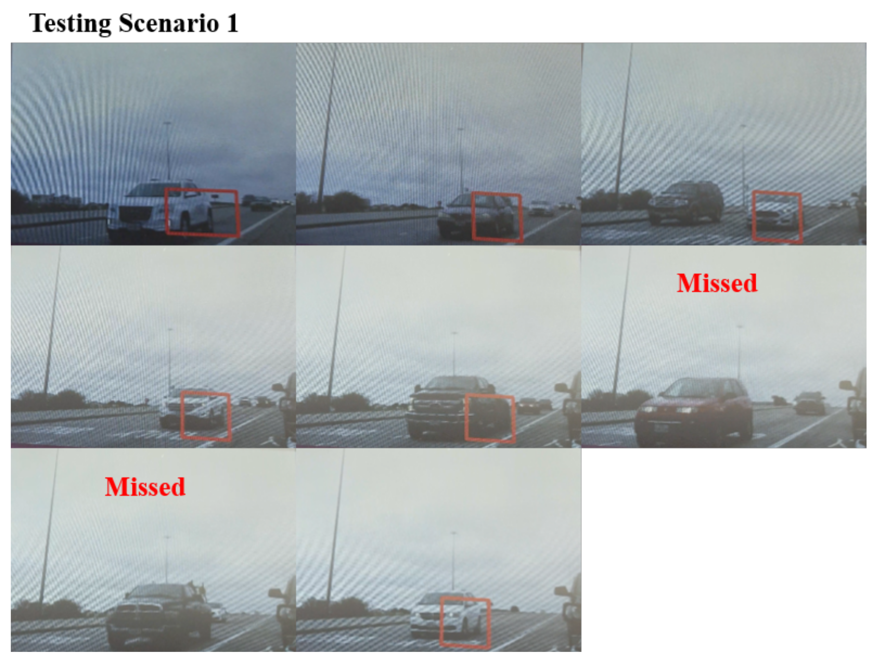
5. Experiments on a Real Road

The first job to test the system on a road is code deployment, and an off-the-shelf embedded board was adopted for this. Detailed hardware specifications and system architecture of this embedded board are depicted in Figure 11.

A USB 2.0, 720 px High Definition resolution, and 30 Frames per Second (FPS) supportive camera was connected to the board, and this camera was mounted on the passenger side mirror. Note that when we tested the mounted camera before actual testing on a road, there was no serious latency. In addition, the 7" LCD display was connected to the board, and this screen was mounted on the dash board. Testing was conducted on a cloudy day with consideration of various factors such as vehicle types, vehicle colors, camera angles, and vehicle speed. In addition, hyperparameters to maximize detection accuracy and minimize false positives for testing on the embedded board changed as follows:

• the size of a rectangle box: 6000
• the threshold value: 2
• the size of detection memory: 10

We drove approximately 40 Miles Per Hour (MPH) on a local road and highway for about 90 min to see whether the developed system could detect all types of vehicles, such as a passenger sedan, Sports Utility Vehicle (SUV), pick up truck, van, and semi-trailer, well based on previously defined scenarios. Experimental results are quite interesting, and no system failure was found during testing. To test the first scenario, in which the system-equipped vehicle stopped or moved more slowly than target vehicles, we stopped on a local road to wait for traffic signal. Eight target vehicles passed the system equipped-vehicle in the next lane, and types and colors of the target vehicles were: two white SUVs, one grey sedan, one white sedan, two black pick up trucks, one red SUV, and one white van. We could not mechanically measure the speed of the passing vehicles, but our intuitive feeling was 35 MPH. The system showed 75% detection accuracy as six vehicles were correctly detected, but the system missed two vehicles. No false positives were reported in these experiments.

For the second scenario, in which the system-equipped vehicle moved more quickly than target vehicles, we tested the system on a local road and highway. Our vehicle passed one black pick up truck on a local road at a speed of 35 MPH and one red, blue, and white semi-trailer on a highway at a speed of 75 MPH. We passed one grey hatchback on a highway at a speed of 75 MPH as well but, after passing this vehicle, we kept a distance between the system-equipped vehicle and grey hatchback. Note that both vehicles were driving at a speed of 75 MPH. In the experiments with the black pick up truck on a local road, the system correctly detected the truck without any false positives, thus that detection accuracy was 100%. The system showed 100% detection accuracy for all three semi-trailers, but there were two false positives, which detected a pole and traffic sign as vehicle features. In the last experiments with a grey hatchback, this vehicle was detected correctly with 100% detection accuracy, but there was one false positive, which detected a lane as a vehicle feature. We found that the video quality in the LCD display through the mounted camera did not affect the results.

Table 3. Summary of experimental results on a real road.

Scenarios	Detection Accuracy	False Positives
When target vehicles passed the system-equipped vehicle at a speed of 35 MPH	75%, Two vehicles out of eight vehicles were missed	No false positives
When the system-equipped vehicle passed a black pick up truck at a speed of 35 MPH	100%	No false positives
When the system-equipped vehicle passed three semi-trailers at a speed of 75 MPH	100%	2 false positives
When the system-equipped vehicle was driving at a same speed of 75 MPH with a grey hatchback	100%	1 false positive

shows a summary of experimental results on a real road, and Figure 12 and Figure 13 show recorded experimental results captured by a mobile device based on all scenarios described in Table 3.

6. Conclusions, Limitations, and Future Work

In this research, we developed a camera-based vehicle blind spot detection system through the FCN. The established research framework was composed of five stages: data preprocessing, feature extraction, FCN model learning, vehicle blind spot setting, and false positive reduction. Overall, 99.45% training accuracy and 98.99% testing accuracy of the FCN model were achieved, respectively. After deploying the software on the embedded board for actual testing on a real road, we confirmed 93.75% average blind spot detection accuracy with three false positives. The main expected effect is commercialization, which may replace the existing radar sensor-based blind spot detection system so that cost saving can be expected from the view point of the automobile manufacturer. In addition, this developed system can be applied to future autonomous vehicles.

However, we encountered a set of limitations through conducting this research. The first research limitation refers to image datasets. Not enough images were extracted and preprocessed, and our own image datasets could not be secured due to time constraints. Testing with live video images was the second research limitation. Testing accuracy with live video images should have been evaluated mechanically similar to training and testing accuracy on the cloud platform, and we are still finding a way for this. In addition, testing was not conducted on a variety of weather conditions. The third research limitation was performance of the system. Although the system showed more satisfactory performance than our expectations, we are eager to show 100% guaranteed system performance without any false positives. The last and biggest research limitation was that we did not apply representation/feature learning and adopt any other deep learning methodologies such as CNN, Recurrent Neural Network (RNN), etc. for comparison analysis. All these research limitations would be future research work as described below.

• More than ten thousand images including vehicles, motorcycles, and any other non-vehicle objects will be secured for both training and testing. By doing so, training and testing accuracy of a deep learning model will be improved. In addition, the system will be optimized for no false positives.
• One of the issues during system testing was that camera angles continuously changed due to a strong wind while the vehicle was driving at high speed. Furthermore, image quality from the camera was not good enough. Hence, a camera which has better hardware specifications will be mounted with fixed angles underneath the side mirror, and further experiments under various conditions will be conducted. In addition, two cameras on both sides will be adopted for testing.
• Target vehicles were detected by a rectangle box, but this would be replaced with a blind spot icon. Specifically, this icon will be displayed on the screen when target vehicles are detected in the blind spot. Moreover, the system will give both visual and audible alarms.
• The reason for employing the FCN model in this research was that the adopted off-the-shelf embedded board had the power limit, thus this resulted in fewer cores and less parallelization. Due to this constraint, we decided to experiment the simplest one among a variety of deep learning methodologies. Moreover, the total amount of the images to be processed for classification was reduced by the sliding window technique. Since our goal was to identify the features of a vehicle in a particular area within a given image, this remarkably reduced the need of having complex networks with enhanced classification capabilities. However, it is highly meaningful to compare and analyze differences from the system developed on FCN basis by adopting different deep learning methodologies, so a new vehicle blind spot detection system will be developed by adopting various deep learning methodologies.
• To make fewer and faster computations on the embedded board, we skipped representation learning. However, we believe that a different approach to handle dimensionality curse was taken. As mentioned above, the sliding window technique used to identify the features of a vehicle was applied to only process the blind spot area. A relatively small rectangular window was processed at the overlapping horizontal and vertical locations of the image. It is important to note that the size of window is much smaller than the size of a vehicle in blind spot. In addition, a heat map was created out of all the windows identifying features. The rectangular localization was obtained out of the heat map pixels having heat beyond a threshold level. This not only helped to overcome dimensionality curse, but also required substantially less computation power because matrix multiplications could be done on a smaller matrix. However, it is also worthwhile to employ a methodology such as the RBMs to see how representation/feature learning can change the processing of our model.

References

1. Yeomans, G. Autonomous vehicles: handing over control—Opportunities and risks for insurance. Lloyds 2014, 18, 4–23. [Google Scholar]
2. Litman, T. Autonomous Vehicle Implementation Predictions; Victoria Transport Policy Institute: Victoria, CO, Canada, 2017. [Google Scholar]
3. National Transportation Safety Board (NTSB). Highway Accident Report: Collision between a Car Operating with Automated Vehicle Control Systems and a Tractor-Semitrailer Truck; NTSB: Washington, DC, USA, 2016. [Google Scholar]
4. Brown, B.; Laurier, E. The trouble with autopilots: Assisted and autonomous driving on the social road. In Proceedings of the 2017 CHI Conference on Human Factors in Computing Systems, Denver, CO, USA, 6–11 May 2017; pp. 416–429. [Google Scholar]
5. Bulumulle, G.; Bölöni, L. Reducing Side-Sweep Accidents with Vehicle-to-Vehicle Communication. J. Sens. Actuator Netw. 2016, 5, 19. [Google Scholar] [CrossRef]
6. Schneider, M. Automotive radar–status and trends. In Proceedings of the German Microwave Conference, Ulm, Germany, 5–7 April 2005; pp. 144–147. [Google Scholar]
7. Hasch, J. Driving towards 2020: Automotive radar technology trends. In Proceedings of the Microwaves for Intelligent Mobility (ICMIM), Heidelberg, Germany, 27–29 April 2015; pp. 1–4. [Google Scholar]
8. Forkenbrock, G.; Hoover, R.L.; Gerdus, E.; Van Buskirk, T.R.; Heitz, M. Blind Spot Monitoring in Light Vehicles—System Performance; Technical Report; National Highway Traffic Safety Administration: Washington, DC, USA, 2014. [Google Scholar]
9. Oshida, K.; Watanabe, T.; Nishiguchi, H. Vehicular Imaging Device. USA Patent 9,294,657, 22 March 2016. [Google Scholar]
10. Sotelo, M.Á.; Barriga, J.; Fernández, D.; Parra, I.; Naranjo, J.E.; Marrón, M.; Alvarez, S.; Gavilán, M. Vision-based blind spot detection using optical flow. In Proceedings of the International Conference on Computer Aided Systems Theory, Las Palmas de Gran Canaria, Spain, 12–16 February 2007; pp. 1113–1118. [Google Scholar]
11. Saboune, J.; Arezoomand, M.; Martel, L.; Laganiere, R. A visual blindspot monitoring system for safe lane changes. In Proceedings of the International Conference on Image Analysis and Processing, Ravenna, Italy, 14–16 September 2011; pp. 1–10. [Google Scholar]
12. Jung, K.H.; Yi, K. Vision-based blind spot monitoring using rear-view camera and its real-time implementation in an embedded system. J. Comput. Sci. Eng. 2018, 12, 127–138. [Google Scholar] [CrossRef]
13. Zhao, Y.; Bai, L.; Lyu, Y.; Huang, X. Camera-Based Blind Spot Detection with a General Purpose Lightweight Neural Network. Electronics 2019, 8, 233. [Google Scholar] [CrossRef]
14. Krause, J.; Stark, M.; Deng, J.; Fei-Fei, L. 3D Object Representations for Fine-Grained Categorization. In Proceedings of the 4th International IEEE Workshop on 3D Representation and Recognition (3dRR-13), Sydney, Australia, 2 December 2013. [Google Scholar]
15. Geiger, A.; Lenz, P.; Stiller, C.; Urtasun, R. Vision meets Robotics: The KITTI Dataset. Int. J. Robot. Res. 2013, 32, 1231–1237. [Google Scholar] [CrossRef]
16. Arróspide, J.; Salgado, L.; Nieto, M. Video analysis-based vehicle detection and tracking using an mcmc sampling framework. EURASIP J. Adv. Signal Process. 2012, 2012, 2. [Google Scholar] [CrossRef]
17. Uhm, D.; Jun, S.H.; Lee, S.J. A classification method using data reduction. Int. J. Fuzzy Log. Intell. Syst. 2012, 12, 1–5. [Google Scholar] [CrossRef]
18. Chao, W.L. Dimensionality Reduction; Graduate Institute of Communication Engineering, National Taiwan University: Taipei City, Taiwan, 2011. [Google Scholar]
19. Kwon, D.; Kim, H.; Kim, J.; Suh, S.C.; Kim, I.; Kim, K.J. A survey of deep learning-based network anomaly detection. Clust. Comput. 2017, 1–13. [Google Scholar] [CrossRef]
20. Ngiam, J.; Khosla, A.; Kim, M.; Nam, J.; Lee, H.; Ng, A.Y. Multimodal deep learning. In Proceedings of the 28th International Conference on Machine Learning (ICML-11), Washington, DC, USA, 28 June–2 July 2011; pp. 689–696. [Google Scholar]
21. Nam, J.; Herrera, J.; Slaney, M.; Smith, J.O. Learning Sparse Feature Representations for Music Annotation and Retrieval. In Proceedings of the 13th International Society for Music Information Retrieval Conference, Porto, Portugal, 8–12 October 2012; pp. 565–570. [Google Scholar]
22. Mousas, C.; Anagnostopoulos, C.N. Learning Motion Features for Example-Based Finger Motion Estimation for Virtual Characters. 3D Res. 2017, 8, 25. [Google Scholar] [CrossRef]
23. Bengio, Y.; Courville, A.; Vincent, P. Representation learning: A review and new perspectives. IEEE Trans. Pattern Anal. Mach. Intell. 2013, 35, 1798–1828. [Google Scholar] [CrossRef]
24. Churchill, M.; Fedor, A. Histogram of Oriented Gradients for Detection of Multiple Scene Properties. 2014. [Google Scholar]
25. Dalal, N.; Triggs, B. Histograms of oriented gradients for human detection. In Proceedings of the 2005 IEEE Computer Society Conference on Computer Vision and Pattern Recognition (CVPR’05), San Diego, CA, USA, 20–25 June 2005; Volume 1, pp. 886–893. [Google Scholar]
26. Sze, V.; Chen, Y.H.; Yang, T.J.; Emer, J.S. Efficient processing of deep neural networks: A tutorial and survey. Proc. IEEE 2017, 105, 2295–2329. [Google Scholar] [CrossRef]
27. Krizhevsky, A.; Sutskever, I.; Hinton, G.E. Imagenet classification with deep convolutional neural networks. In Proceedings of the Advances in Neural Information Processing Systems, Lake Tahoe, NV, USA, 3–6 December 2012; pp. 1097–1105. [Google Scholar]
28. He, K.; Zhang, X.; Ren, S.; Sun, J. Deep residual learning for image recognition. In Proceedings of the IEEE Conference on Computer Vision and Pattern Recognition, Las Vegas, NV, USA, 26 June–1 July 2016; pp. 770–778. [Google Scholar]
29. Abdi, M.; Nahavandi, S. Multi-residual networks: Improving the speed and accuracy of residual networks. arXiv 2016, arXiv:1609.05672. [Google Scholar]
30. Cho, K.; Van Merriënboer, B.; Gulcehre, C.; Bahdanau, D.; Bougares, F.; Schwenk, H.; Bengio, Y. Learning phrase representations using RNN encoder-decoder for statistical machine translation. arXiv 2014, arXiv:1406.1078. [Google Scholar]
31. Jiang, S.; de Rijke, M. Why are Sequence-to-Sequence Models So Dull? Understanding the Low-Diversity Problem of Chatbots. arXiv 2018, arXiv:1809.01941. [Google Scholar]
32. Rekabdar, B.; Mousas, C.; Gupta, B. Generative Adversarial Network with Policy Gradient for Text Summarization. In Proceedings of the 2019 IEEE 13th International Conference on Semantic Computing (ICSC), Newport Beach, CA, USA, 30 January–1 February 2019; pp. 204–207. [Google Scholar]
33. Kim, M.; Lee, W.; Yoon, J.; Jo, O. Building Encoder and Decoder with Deep Neural Networks: On the Way to Reality. arXiv 2018, arXiv:1808.02401. [Google Scholar]
34. Ng, A. CS229 Lecture Notes; 2000; Volume 1, pp. 1–3. Available online: https://www.researchgate.net/publication/265445023_CS229_Lecture_notes (accessed on 20 July 2019).
35. Minski, M.L.; Papert, S.A. Perceptrons: An Introduction to Computational Geometry; MIT Press: Cambridge, MA, USA, 1969. [Google Scholar]
36. Werbos, P.J. The Roots of Backpropagation: From Ordered Derivatives to Neural Networks and Political Forecasting; John Wiley & Sons: Hoboken, NJ, USA, 1994; Volume 1. [Google Scholar]
37. Rumelhart, D.E.; Hinton, G.E.; Williams, R.J. Learning representations by back-propagating errors. Nature 1986, 323, 533–536. [Google Scholar] [CrossRef]
38. LeCun, Y.; Bengio, Y.; Hinton, G. Deep learning. Nature 2015, 521, 436–444. [Google Scholar] [CrossRef]
39. Barter, R.L.; Yu, B. Superheat: An R package for creating beautiful and extendable heatmaps for visualizing complex data. arXiv 2015, arXiv:1512.01524. [Google Scholar] [CrossRef]
40. Samek, W.; Binder, A.; Montavon, G.; Lapuschkin, S.; Müller, K.R. Evaluating the visualization of what a deep neural network has learned. IEEE Trans. Neural Netw. Learn. Syst. 2017, 28, 2660–2673. [Google Scholar] [CrossRef]
41. Senthilkumaran, N.; Vaithegi, S. Image segmentation by using thresholding techniques for medical images. Comput. Sci. Eng. Int. J. 2016, 6, 1–13. [Google Scholar] [CrossRef]
42. Chaubey, A.K. Comparison of The Local and Global Thresholding Methods in Image Segmentation. World J. Res. Rev. 2016, 2, 1–4. [Google Scholar]
43. Von Zitzewitz, G. Deep Learning and Real-Time Computer Vision for Mobile Platforms. Available online: https://www.researchgate.net/publication/331839269_Deep_Learning_and_Real-Time_Computer_Vision_for_Mobile_Platforms (accessed on 20 July 2019).
Figure 1. Radar module of the blind spot detection system.
Applsci 09 02941 g001
Figure 2. Camera-based blind spot system.
Applsci 09 02941 g002
Figure 3. Example of vehicle images.
Applsci 09 02941 g003
Figure 4. Camera installation for preliminary testing.
Applsci 09 02941 g004
Figure 5. Example of the extracted images.
Applsci 09 02941 g005
Figure 6. Data visualization of the vehicle and non-vehicle images.
Applsci 09 02941 g006
Figure 7. Example of HOG feature extraction for the vehicle and non-vehicle object.
Applsci 09 02941 g007
Figure 8. Blind spot setting zone.
Applsci 09 02941 g008
Figure 9. Overall research framework. A total of 2000 vehicle images and approximately 9000 non-vehicle images were extracted for the purpose of data preprocessing. The HOG descriptor was applied for feature extraction, and 1188 HOG features for both vehicle and non-vehicle objects were fed into the FCN model as inputs. Keep in mind that representation or feature learning was not applied in this research due to hardware constraints. Two hidden layers, 1 × 10 6 learning rate, and 10 epochs with Adam optimizer and ReLus activation were employed for training and testing the FCN model, and the training and testing accuracies achieved were 99.4% and 99.0%, respectively. We set a blind spot to a range of 400–800 px in x-axis and 450–550 px in y-axis in the 1300 px × 800 px image and applied the sliding window technique to detect vehicle features. Finally, the heat map and thresholding were employed to reduce false positive errors.
Applsci 09 02941 g009
Figure 10. Experimental results of both scenarios.
Applsci 09 02941 g010
Figure 11. System architecture of the embedded board: The embedded board comes with 64-bit Quad-Core and Dual-Core CPU clusters, a GPU with 256 Compute Unified Device Architecture (CUDA) cores, and 8 GB 128-bit LPDDR4 RAM. The main purpose and advantage of this embedded board is used for embedded AI platform with speed and power efficiency [43], but to use a variety of features offered by the embedded board, a lot of software packages should be installed.
Applsci 09 02941 g011
Figure 12. Experimental result of the first testing scenario.
Applsci 09 02941 g012
Figure 13. Experimental result of the second testing scenario.
Applsci 09 02941 g013