Article

Multi Simulation Platform for Time Domain Diffuse Optical Tomography: An Application to a Compact Hand-Held Reflectance Probe

1
Politecnico di Milano, Dipartimento di Fisica, Piazza Leonardo da Vinci, 32, 20133 Milan, Italy
2
Consiglio Nazionale delle Ricerche, Istituto di Fotonica e Nanotecnologie, Politecnico di Milano, Piazza Leonardo da Vinci, 32, 20133 Milan, Italy
3
Department of Computer Science, University College London, Gower Street, London WC1E 6BT, UK
4
Dipartimento di Fisica e Astronomia, Università degli Studi di Firenze, Via G. Sansone 1, 50019 Sesto Fiorentino, Firenze, Italy
*
Author to whom correspondence should be addressed.
Appl. Sci. 2019, 9(14), 2849; https://doi.org/10.3390/app9142849
Submission received: 24 May 2019 / Revised: 3 July 2019 / Accepted: 15 July 2019 / Published: 17 July 2019

Abstract

:

Featured Application

The present work represents a preliminary performance assessment of a simulated system for Time Domain Diffuse Optical Tomography, in view of the upcoming development of a real system for breast cancer imaging, which shall feature a reduced number of sources and detectors, compact silicon-based detectors, and that shall avoid exceedingly long breast examination times. These features make the proposed system suitable to be integrated into a compact hand-held probe for breast lesion characterization (malignant vs. benign). To improve the reconstructions, morphological information will be provided by ultrasound imaging, integrating an ultrasound transducer in the probe along with the TD-DOT instrumentation.

Abstract

Time Domain Diffuse Optical Tomography (TD-DOT) enables a full 3D reconstruction of the optical properties of tissue, and could be used for non-invasive and cost-effective in-depth body exploration (e.g., thyroid and breast imaging). Performance quantification is crucial for comparing results coming from different implementations of this technique. A general-purpose simulation platform for TD-DOT clinical systems was developed with a focus on performance assessment through meaningful figures of merit. The platform was employed for assessing the feasibility and characterizing a compact hand-held probe for breast imaging and characterization in reflectance geometry. Important parameters such as hardware gating of the detector, photon count rate and inclusion position were investigated. Results indicate a reduced error (<10%) on the absorption coefficient quantification of a simulated inclusion up to 2-cm depth if a photon count rate ≥ 106 counts per second is used along with a good localization (error < 1 mm down to 25 mm-depth).

1. Introduction

Medical imaging often employs tomography as an effective tool to help detecting and characterizing both pathological and physiological conditions in tissues. Tomography provides 2D/3D images of the tissue under investigation and is performed exploiting approaches that typically involve ionizing radiations or complex magnetic field analysis (e.g., X-Ray CT, MRI).
A different non-invasive experimental approach involves injecting low-power laser light in the Near-Infrared (NIR) spectrum and studying photon paths through the tissue to derive its optical properties, i.e., absorption and scattering. Thus, performing optical measurements with a set of properly arranged sources and detectors enables a full 3D reconstruction of the optical properties that correlate with the nature of imaged tissue. Such an approach is known as Diffuse Optical Tomography (DOT), because light propagation follows a quasi-diffusion like model when working in the NIR on large (cm3) tissue volumes (e.g., for clinical applications). Other approaches involve the detection of the diffused fluorescence signal (Fluorescence DOT) emitted by a specific fluorescent marker after being injected into the tissue [1].
Specifically, Time Domain DOT (TD-DOT) is performed by injecting pulsed laser light and detecting the effects of propagation through the tissue (i.e., amplitude attenuation, delay and temporal broadening of the pulse) to retrieve the optical properties of the tissue [2].
TD-DOT is potentially powerful for applications needing in-depth body exploration (such as brain activation [3], thyroid and breast imaging), and can be implemented in compact hand-held probes for easier non-invasive clinical examinations [4]. The main advantage of the TD approach is that it enables one to uncouple the effects of scattering from the effects of absorption in a single measurement, with no need for multiple distance measurements. Furthermore, when reflectance geometry is used, the photon Time-of-Flight (TOF) provides information on the depth probed by the measurement. More generally, the TD approach, exploiting time as an additional dimension, reduces —at least in principle—the required number of sources and detectors with respect to continuous wave or frequency domain operation, and that enables simpler implementations for medical use [5].
In the last years an important technology push has made the TD approach more attractive: Detectors like Silicon Photomultipliers (SiPMs), adapted from different applications, proved to be cheaper, more compact and sensitive than conventional detectors (e.g., Photomultiplier Tubes) and started to be widely applied as single-photon detectors in optical measurements [4,6]. At the same time, SiPMs can be developed for hardware gating of the photon distribution, thus opening to higher penetration depths, but still keeping small dimension, which is not trivial for gated detectors [5].
Despite recent technology innovations, there is plenty of room for improvement in TD-DOT in reflectance geometry on the software side (e.g., reconstruction algorithms), as well as on the hardware side (e.g., more compact multiwavelength or tunable sources). Thus, anticipating a consistent framework for this modality, a clear and widely shared approach to performance quantification is essential for comparing results from different implementations, driving improvements in hardware and data analysis, and anticipating problems that may arise in the clinical environment.
Breast cancer applications are crucial, as it is the most common cancer amongst women, with about 1 in 8 females being diagnosed with the disease during their lifetime [7,8]. Survival rate significantly improves when an early diagnosis is reached. Nowadays screening mammograms play a key role in the prevention programs, but X-ray mammography still suffers from a low sensitivity that generally leads to unnecessary, social-care expensive, painful and invasive examinations [9,10]. Apart from Magnetic Resonance Imaging (MRI) [11,12] and Ultrasound (US) imaging [13,14], that are already applied in clinics as supplementary imaging tools, several techniques are presently being investigated for the quantitative imaging of breast cancer [15]. Among them, a hand-held optical probe for TD-DOT could prove useful to improve diagnostic sensitivity, performing non-invasive, cheap and physiological-related examinations to better characterize and classify breast lesions after a positive screening mammography.
The purpose of the paper is twofold. First, we present a simulation platform suitable for simulations of large multi-parameter scenarios in DOT, and then we exploit this platform for a systematic study of the performances and feasibility of a TD-DOT hand-held probe to work in reflectance geometry for breast cancer imaging and characterization. More in detail, the key features and the novelty of the platform are: (i) Fully automated scheme which permits to run automatically large multi-parametric scenarios in batch processing; (ii) an objective, quantitative and operator-independent assessment of the outcome of the reconstruction in view of the desired clinical application; (iii) attempt to enforce standardization and performance assessment criteria, following internationally agreed protocols (e.g., BIP [16], MEDPHOT [17], NEUROPT [18]). As compared to existing tomographic packages (e.g., TOAST [19] or NIRFAST [20]) our platform does not offer novelty in the algorithms, but rather aims at studying automatically and with an objective and quantitative outcome the effects of different parameters in a flexible and systematic way.
The second aim of the paper is to exploit the simulation platform to investigate TD-DOT in reflectance geometry with a limited set of source-detector couples towards applications for breast diagnostics. Many parameters with a complex interplay were considered simultaneously, at the level of hardware implementation (number and temporal width of the time gates, counts per second), experimental conditions (depth of the absorption inhomogeneity), and reconstruction parameters (regularization, voxel size). Also, an objective quantification of the tomography reconstruction is needed to assess the capability of the system to classify different lesions. The results will display the limits of applicability, the expected performances, and the key bottlenecks of such a compact 3D probe with respect to realistic scenarios.
The rest of this paper is organized as follows: In Section 2 we present the architecture of the developed multipurpose simulation platform, followed by a detailed discussion about the specific kernel for time domain breast tomography, with problem specifications. Finally, we describe the systematic set of simulations we performed for investigating a wide combination of variables. In Section 3 we report the main results we obtained along with the accuracy in the estimate of optical parameters.

2. Materials and Methods

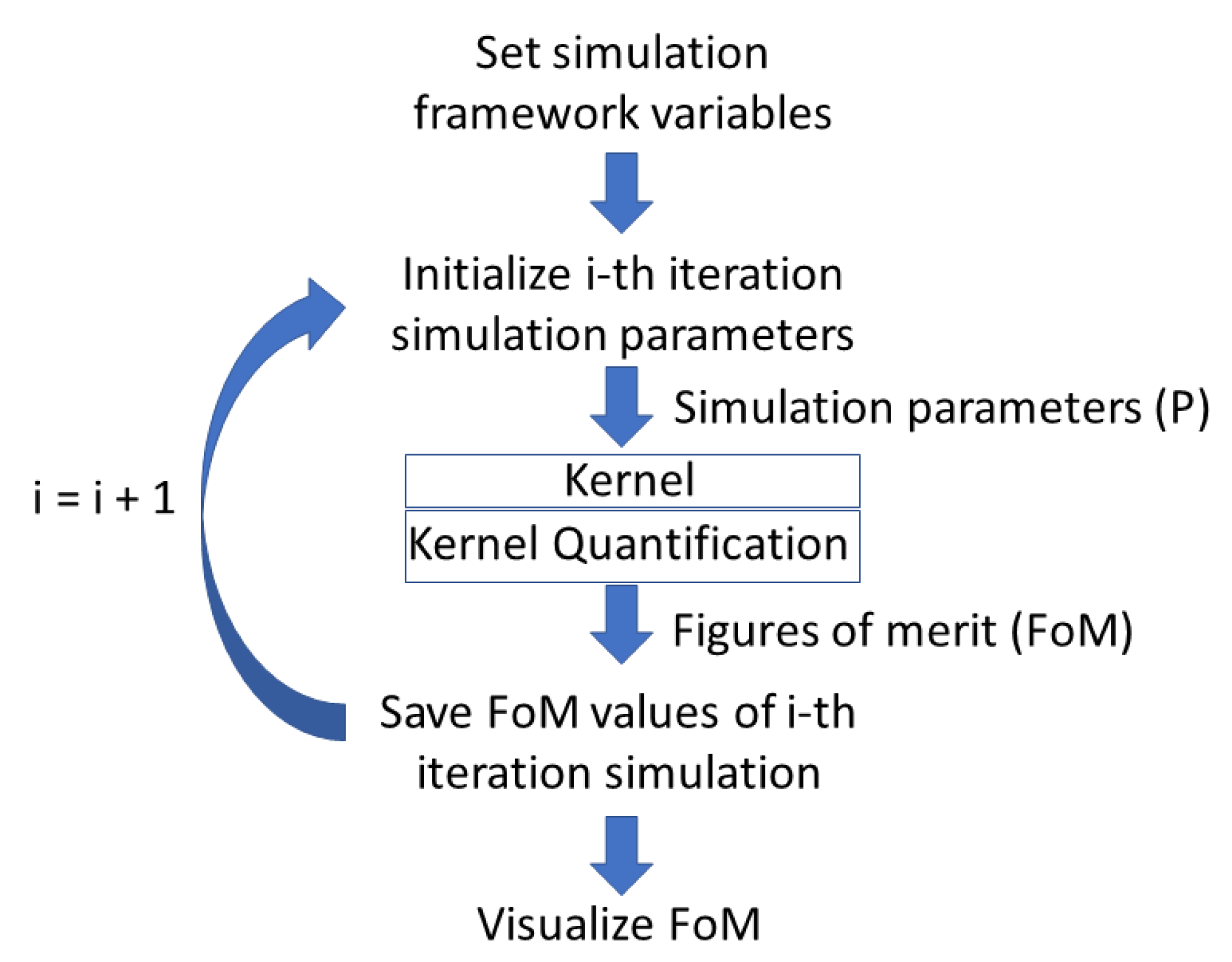
2.1. Multi Simulation Platform

The (Matlab®-based) simulation platform was developed to perform systematic simulations mimicking realistic instrumentation for different kinds of applications (simulation kernel), and a generic software architecture was exploited to build a flexible and multipurpose tool. At the same time, we focused on the quantitative assessment of the outcomes and on their comprehensive visualization to help better understand system performances. Quantification is reached by the identification either of some meaningful characteristics or figure of merit (FoM) that well describe system performances, or by comparison with what is defined in well-established standardization protocols. Finally, a visualization section provides a graphical representation of FoMs when up to 5 parameters are changed in the simulations.
Figure 1 depicts the software architecture. The scheme can be divided into 5 main parts:
  • Setting of the simulation framework variables;
  • Simulation parameters update and override onto the default values;
  • The kernel: The single-shot simulation core code for the specific application the user wishes;
  • Quantification and extraction of the FoMs;
  • Visualization of the FoMs.
The first step is to set the entire variables framework the user wishes to use for the simulation batch and flag only those for which the user wants to study a specific range of values. The space of variables is described in an abstract way, so that the user can decide for each variable either to fix a constant value, or to specify a range of discrete values. For up to five independent variables, the program will study all possible combinations of values in the range.
The number of total iterations of the kernel code is given by the product of the numericity of the flagged variables. Each iteration thus corresponds to a specific combination of the values of the flagged variables. The values of all the variables are set just before the kernel runs.
At the end of each iteration, FoMs are calculated and stored for following visualization.

2.2. Tomographic Kernel

The kernel is divided into two sections: (i) Forward problem and (ii) Inverse problem.
For the forward problem, analytical solutions to the Diffusion Equation under Extrapolated Boundary Conditions for a semi-infinite medium have been computed both for the homogeneous case and for the heterogeneous case. In the latter case, a perturbative solution under the Born approximation has been used over a voxelated volume [21]. Notwithstanding the large availability of more sophisticated models, such as finite-elements (FEM) [22] or Monte-Carlo [23,24], the use of an analytical solution has the advantage to be quite faster than numerical methods, and to be independent of the temporal discretization. After the computation of the forward time-resolved curves, they are converted to photon-counts, accordingly to the desired count-rate, responsivity of the system, measurement time, source/detector areas, and source power. More in detail: the fluence is translated to actual photon counts, considering an average injection power of 1 mW at 800 nm. The acquisition time is set to 1 s, while the detectors are simulated with a 7 mm2 active area and a 0.04 quantum efficiency. The simulated values represent a realistic estimate based on actual system setups. No optical losses are considered, since the detector is supposed to be in contact with the medium with full acceptance angle. These figures are used to estimate the maximum number of detected photons. Then, to account for the maximum count rate sustainable for the detection electronics, that number is clipped to an upper limit (typically, this value is 106 counts per second). If desired, an experimentally-derived Instrumental Response Function (IRF) can also be convolved to all the curves for simulating a specific detector. Afterwards, multiplicative Gaussian noise (0.1%) is added to take into account amplitude fluctuations and in general other instabilities of the system. Finally, Poisson noise is added to simulate the shot noise associated with photon detection. The two types of noise simulate the modification of an ideal distribution of time of flight due to the non-ideal experimental setup (Gaussian noise) and photon detection (Poisson noise). More details can be found in [5]. In particular, measurements with a gated detector can be also simulated [25].
Concerning the reconstruction of the absorption coefficient ( μ a ) in the volume, a Jacobian matrix is first computed by solving the following time convolution [21]:
J ( r i , t k ; r s , r d ) = t k t k + Δ t G ( r s , r i , t ) G ( r i , r d , t ) h ( t ; r s , r d ) d t ,
where ri is the position of the ith voxel, t k is the kth Δ t broad temporal window, r s and r d the source/detector position, respectively, G ( r l , r m , t ) is the Green’s Function for the semi-infinite medium calculated at the position r m for a source placed at r l , and h ( t ; r s , r d ) is the IRF related to the source/detector pairs placed at r s and r d . The first convolution between the Green’s functions has been analytically solved to speed up the calculation [21].
The distribution of the absorption perturbation with respect to the background optical properties is retrieved by solving the following problem:
Δ μ a = a r g min Δ μ a { i ( y i J i Δ μ a σ i ) 2 + τ Δ μ a 2 } ,
where Δ μ a is the vector of the absorption perturbations in each voxel ( Δ μ a = μ a p e r t u r b a t i o n μ a b a c k g r o u n d ), yi is the simulated photon-count in each time window and for every source/detector pairs, Ji is the ith row of the Jacobian, σ i = y i is the standard deviation accordingly to the Poisson statistics, and τ is a regularization parameter. Even though the chosen regularization is basic, it provides a solid basis for the future usage of more sophisticated methods, including total variation or l p sparsity [26,27,28,29]. Finally, it is worth noticing that the whole simulated distribution time of flight is used for the reconstruction, thus exploiting the information carried by the time domain data.
Problem (2) is solved by a direct solution of the normal equation:
( J ˜ T J ˜ + τ I ) Δ μ a = J ˜ T y ˜ ,
where J ˜ and y ˜ are the Jacobian matrix and the simulated data vector normalized by standard deviation accordingly to the following:
{ J ˜ = Σ 1 J y ˜ = Σ 1 y ,   Σ = d i a g ( σ i ) ,

2.3. Simulation Overview

For our Time Domain Diffuse Optical Tomography (TD-DOT) simulations in reflectance geometry we used a fixed geometry of sources and detectors placed in a rectangular pattern (30 mm × 20 mm). On each long side of the rectangle 4 pairs of sources and detectors are placed, with overlapping source and detector positions. Spacing between two nearest source-detector pairs is of 10 mm. The simulated probed volume is a parallelepiped (60 mm side and 30 mm) and the rectangular pattern of sources and detectors is located on its top surface. A localized spherical heterogeneity (~5 mm radius, μ a = 0.04 mm−1) is moved within the simulated volume ( μ a = 0.01 mm−1), thus probing the system performances in the region underlying the sources and detectors arrangement. Figure 2 depicts the phantom and measure geometry.
Both sources and detectors are simulated using realistic signal and noise (e.g., source power, Instrument Response Function, detector area and quantum efficiency, and signal noise), mimicking the typical performances of a TD instrument. We modeled the breast as a semi-infinite medium, with a local absorbing perturbation with respect to the background.
To provide a full characterization of our system we performed a thorough series of simulations studying the main parameters that could affect system performances both on the hardware side (e.g., temporal gating) and the software side (e.g., reconstruction parameters). The set of simulations is summarized in Table 1.
Table 2 lists the values of the parameters that have been studied.
Quantification of the simulations outcome is reached through the definition of FoMs:
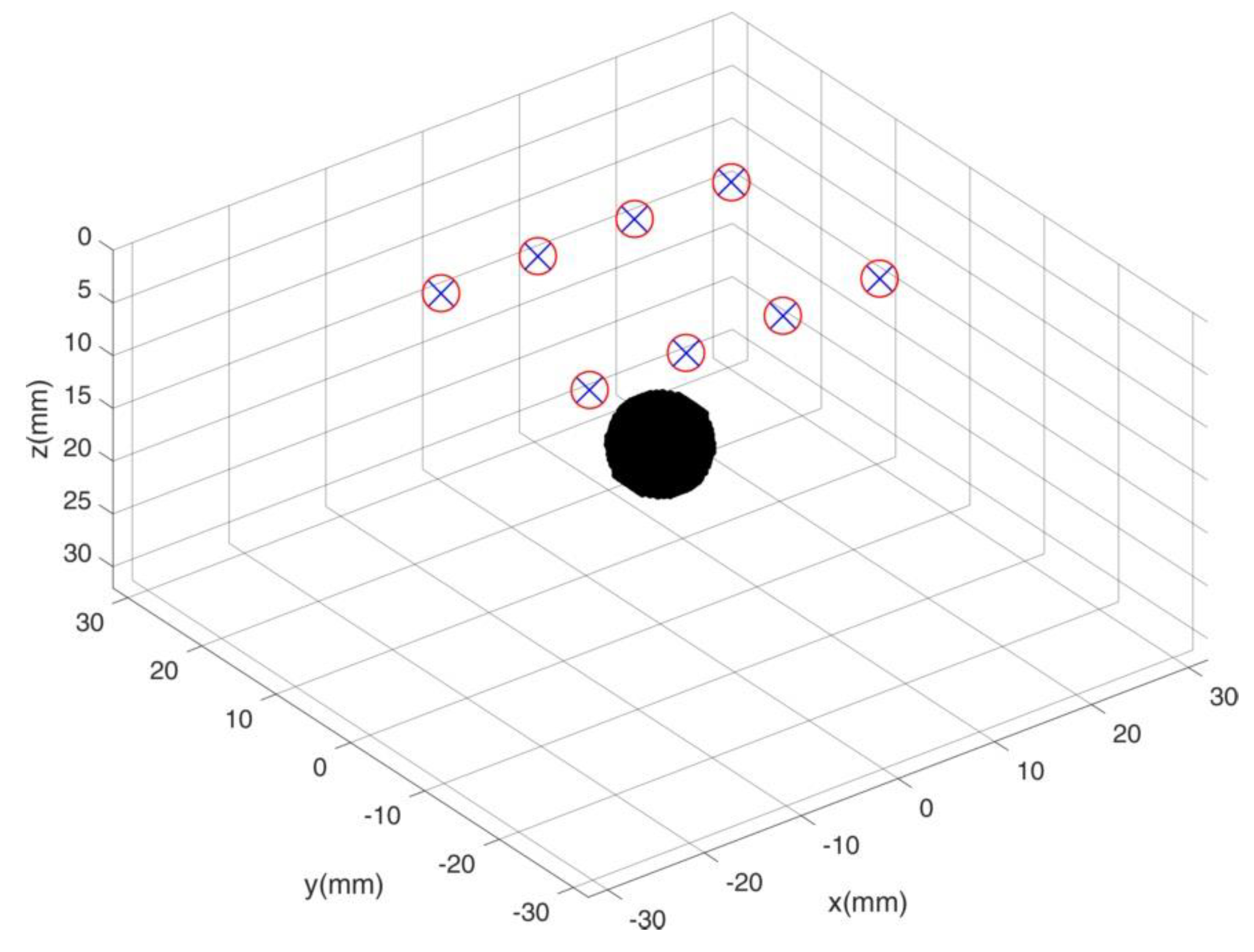
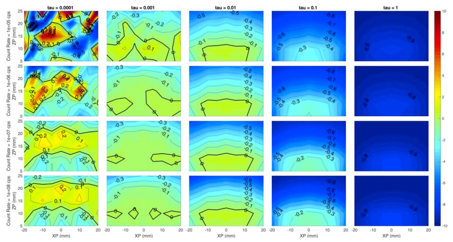
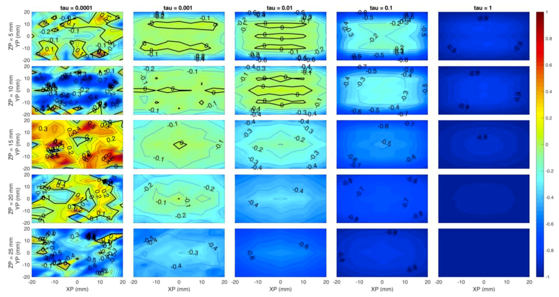
  • The error on the localization of the reconstructed inclusion along the three axes x, y and z with respect to the simulated position according to the center of mass.
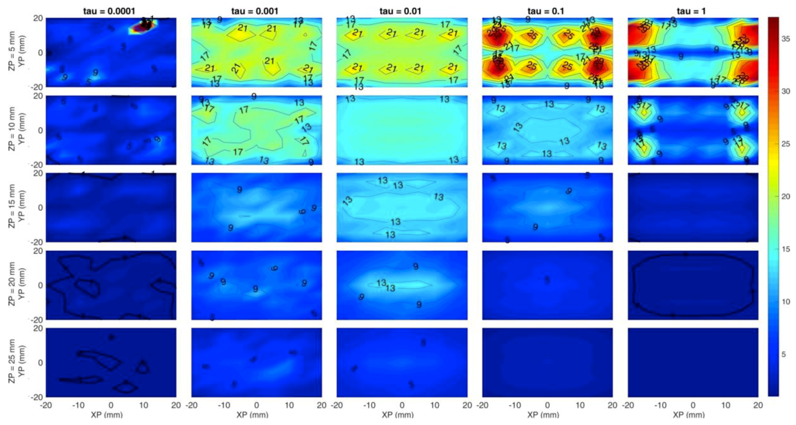
    ϵ l o c = R O I r i r e c R O I r i t r u e i = x , y , z ,
  • The volumetric error on Δ μ a is calculated as:
    ϵ v o l = R O I Δ μ a r e c d V R O I Δ μ a t r u e d V R O I Δ μ a t r u e d V ,
    where ROI is a spherical region of interest (ROI) of radius 2 cm cantered on the center of mass of the reconstructed inclusion and Δ μ a t r u e and Δ μ a r e c are the true and reconstructed absorption perturbation values.
Each simulation set is made of ~2000 independent reconstructions and requested an average of 12 h to complete on a dedicated work station (Dell Precision Tower Workstation 7910, mounting Dual Intel Xeon processors—10 cores, 2.35 GHz—and 64 Gb of RAM memory).

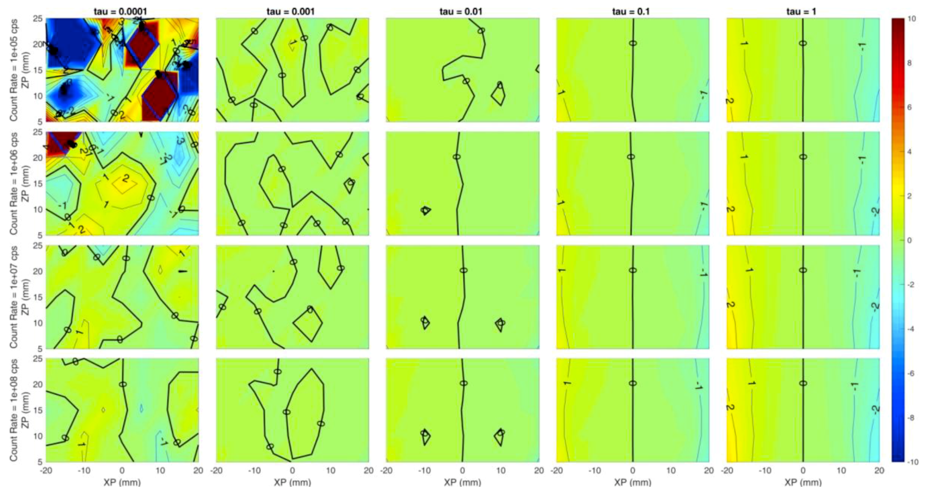
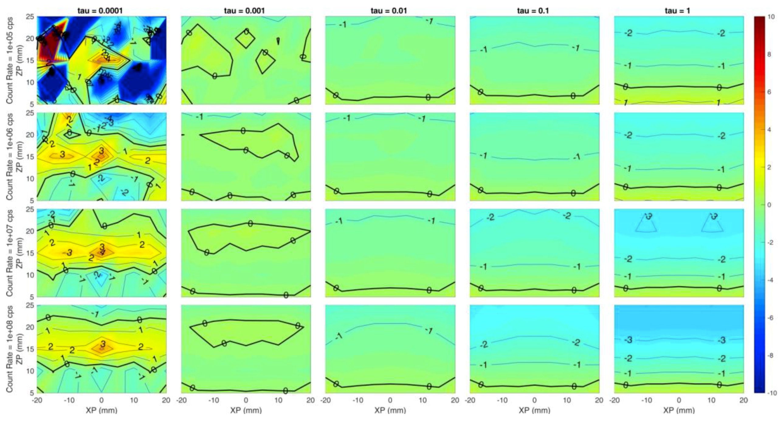
3. Results and Discussion

For the sake of clarity, in the following we will focus on the most meaningful simulations (simulations E and F) and report the main conclusions for the simulations A, B, C and D. For simulations from A to D, we provide external references to FigShare links, which give access to the relative figures that are not reported in this paper, so as not to overload the discussion [30,31,32,33,34,35].
Simulation A has provided indications as for the best voxel size to use during the reconstruction algorithm showing how the 1 mm and 2 mm voxel size are totally equivalent, while the 5 mm voxel size slightly worsens the localization errors and spatial resolution in favor, though, of a significant reduction of calculation time [30,32,35]. We used the 2 mm voxel size for the rest of simulations.
Simulation B showed no significant changes with the Time Channel duration up to 48 ps. A default 12 ps time channel duration was chosen. The number of temporal steps was fixed to be 600, thus leading to a ~7 ns long temporal scale, which fully includes the dynamic range of the simulated curves [33].
Simulation C suggested that the optimal temporal width of the software gating windows should be less than 500 ps. A wider time window introduces errors especially on the absorption coefficient estimation and reduces the penetration depth. The time window duration is given by the duration of the time scale (i.e., the number of time channels multiplied by the time channel duration) divided by the number of time windows. As we fixed the time channel duration to 12 ps and the number of temporal steps to 600, the minimum number of temporal windows is 14: A rounded value of 20 was chosen [31].
Simulation D showed how hardware gating of the detector improves the penetration depth. The relative volumetric error on the absorption coefficient, without gating, is up to 30% at 2 cm depth, while it decreases as close as 10% when several gating windows are used. We identified three as the optimal number of hardware gates: A greater number possibly reduces the photon counts in each window, which may increase error and worsen localization [34].
The previous simulations helped us to define the best variables set to provide a lower absorption quantification error and a better localization of the perturbation. Simulation E is of great interest as it studies the effects of the signal level, which is often a concern in optical breast imaging due to high absorption (e.g., at long wavelengths due to water concentration) and breast thickness variability. In the following we will discuss in detail the figures of merit.
Each panel of Figure 3 shows the error of the reconstructed x coordinate of the inclusion with respect to the simulated one, i.e., the localization on x, expressed in millimeters. The horizontal axis of each panel corresponds to the simulated x coordinate of the inclusion (from −20 mm to 20 mm at 5 mm step), while the Y axis is the depth of the inclusion, i.e., the z coordinate (from 5 mm to 25 mm in 5 mm steps). Different rows correspond to different count rates (105, 106, 107, 108 from top to bottom) while columns represent different values of the regularization parameter (10−4, 10−3, 10−2, 10−1, 10−0 from left to right). The error is color-coded: Red colors correspond to positive errors, while blue colors are negative errors; small errors are identified by greenish colors. The thick black line is the error-free contour line, while a label indicates the error value on the other contour lines.
Figure 3 suggests a general high localization of the x coordinate in most of the conditions as the green color (indicating low error, close to 0 mm) is spread over most of the panels except for low regularization (τ = 10−4). This is expected, as a very small value of the regularization parameter leaves excessive room to the effects of the reconstruction noise. At the same time, the localization error is spatially more uniform for higher regularization: At a fixed count rate, the error dispersion tends to reduce as the contour lines are straighter and zones with different error value are merged together.
However, values exceeding 10−1 could worsen the figure of merit, indicating that a high value of regularization might induce artifacts. The count rate value does not seem to affect the x coordinate localization error for τ ≥ 10−3, as within each column a low error (close to 0 mm) is obtained for every experimented condition. A good localization is achieved even in depth down to 25 mm for τ ≥ 10−3.
The same considerations apply to the localization along the y coordinate (data not shown).
Figure 4 shows the localization on the z coordinate, i.e., the reconstructed z coordinate of the inclusion with respect to the simulated one. Similar conclusion to Figure 3 can be drawn for Figure 4, but it is worth noticing the low localization error (around 0 mm) even in depth (25 mm) for τ = 10−3, which seems to be the best value for the regularization parameter. This is a key aspect as the maximum probed depth is a typical issue when dealing with DO systems, and 25 mm is considered to be a significant value. Moreover, higher regularization values cause the inclusion to be reconstructed at shallower depths, as the negative (blue) error increases for a fixed z coordinate value (same row). As an example, let us consider the last row (count rate = 108 cps) and Zp = 15 mm. The error increases (in absolute value) from 0 mm at τ = 10−3 to −2 mm at τ = 10−1, and reaches −3 mm at τ = 1.
Figure 5 shows the relative volumetric error on the absorption coefficient. The figure clearly highlights that high regularization values cause a negative error—i.e., an underestimation of the absorption coefficient—rapidly increasing with the regularization parameter (i.e., left to right within each row). Again, the best value of τ seems to be 10−3 as the volumetric error is kept as low as 20% (in absolute value), even at 2 cm-depth. Clearly, the error on the quantitation of Δ μ a can be related to the underestimation of z. The regularization tends to attract the perturbation towards the surface and consequently a lower Δ μ a is enough to match the observed contrast. For τ = 10−3, a photon count rate ≥ 106 leads to a wide low-error region (<10%) up to 2 cm depth, which is a positive result as ~106 counts per second (cps) is a realistic signal level.
Figure 6 sums up the previous results and corresponds to simulation F. In this case the Y axis of each subplot is the y coordinate, while rows correspond to a different z coordinate of the inclusion. Count rate is now fixed to 106 cps. A low error region is located within the rectangle identified by sources and detectors positions, and a 2-cm depth can be reached with a ~80% accuracy level in the estimate of the absorption coefficient if a τ = 10−3 is chosen. Higher regularization values cause underestimation of the absorption coefficient as well as worse localization.
Figure 7 is obtained in the same condition as Figure 6, but it shows the Contrast-to-Noise Ratio defined as:
C N R = Δ μ ¯ r e c , r o i Δ μ ¯ r e c , r o i ¯ w r o i σ r o i 2 + w r o i ¯ σ r o i ¯ 2
where Δ μ ¯ r e c , r o i and σ r o i are the mean value and standard deviation of the reconstructed Δ μ a r e c calculated in a region of interest; Δ μ ¯ r e c , r o i ¯ and σ r o i ¯ are calculated on the complementary region of interest ( r o i ¯ = 1 r o i ); w r o i and w r o i ¯ are weights defined as the volume rations w r o i = V r o i V t o t and w r o i ¯ = V r o i ¯ V t o t . The region of interest is defined as the region of space in which the reconstructed Δ μ a r e c is greater than half of the maximum reconstructed value.
This figure of merit is an indicator of the goodness of the reconstruction for specific structures within the volume [36]. The CNR strongly decreases with the depth for any regularization value, but quicker for higher τ values. The column τ = 10 3 and τ = 10 2 provide the best trend for the CNR, leading to a CNR close to 10 at a depth of 2 cm, even though τ = 10 2 seems to offer a more homogeneous distribution at all depths.
Overall, Figure 6 and Figure 7 suggest that the simulated system would be capable of detecting inclusions up to 2 cm depth with a significant accuracy and reasonable contrast.
The previous figures show the spatial distribution of the figures of merit in different experimental conditions (i.e., photon count rate, regularization parameter). However, the most common method of assessing the goodness of a reconstruction is through the cross sections of the overall tomographic image. Thus, in the following Figure 8 and Figure 9, we show an example of the simulated tomography problem and of the obtained reconstruction, respectively. Each subplot corresponds to a different depth (expressed in millimeters) and the X/Y axis is the x/y coordinate in space. The color bar shows the value of the absorption coefficient in mm−1 units. The count rate is fixed at 106 cps and three hardware gates of the detectors are simulated. The regularization parameter is set to 10−2. We simulated the spherical inclusion (whose features are described in Section 2.3) in the center of the x-y plane and at a 10 mm-depth, thus spanning from 5 mm to 15 mm.
The reconstruction in Figure 9 shows small surface artifacts, but the localization in the x-y plane is good as the inclusion is set in the center of such plane, as expected. The z coordinate is reconstructed at a slightly shallower position, as the center of the inclusion is at 9 mm, but the overall height is properly identified. The quantification error is limited to 5%.
All of the presented simulations were carried out at 1 s acquisition time per source-detector pair over the number of hardware gates of the detector. Overall, considering the 64 combinations of the source-detector pair, the measurement time would be around 1 minute. That measurement time was estimated as an acceptable trade-off between the collected signal and measurement duration. Furthermore, different source-detector implementations may allow shorter times. For example, efficient choosing of the most meaningful source-detector pair could reduce the measurement time, at least by a factor of 2.

4. Conclusions

In our work on breast imaging and lesion characterization, we wanted to assess the performances of a Time Domain Diffuse Optical Tomography (TD-DOT) system working in reflectance geometry, formed by eight couples of sources and detectors placed in a rectangular pattern, with a particular focus on the quantification of the system figures of merit. Thus, we developed a general-purpose simulation platform to carry out a quantitative performance assessment of clinical TD-DOT systems. The platform is able to study up to five parameters at the same time and to extract the corresponding figures of merit. It also provides an immediate and concise visualization tool for an analysis and comparison of results. We used the platform to provide a thorough characterization and validation of our TD-DOT system using realistic levels of signal and noise and studying important parameters, such us inclusion position, hardware gating of the detector, regularization parameter ( τ ) and the total photon count rate. The main figures of merit used are the localization error of the reconstructed inclusion with respect to the simulated one and the relative volumetric error on the absorption coefficient.
We found that the hardware gating of the detector significantly improves absorption quantification, enabling one to probe the tissue down to 2 cm-depth with a volumetric error as low as 10%. At the same time a software gating of the reconstructed photon distribution of time of flights improves the penetration depth if the time window is shorter than 500 ps.
Better inclusion localization in the x-y plane (error < 1 mm) was reached under most of the experimented conditions when τ ≥ 10−3 and down to 25 mm-depth in the source-detector rectangular region. The localization error is low along the z axis for τ = 10−3 (error < 1 mm down to 25 mm-depth) but increases with higher values of τ , reaching a −4 mm value when τ = 1. Thus, the inclusion is reconstructed at a shallower depth and there is a strong underestimation of the absorption coefficient. Finally, once we fixed the other parameters, a photon count rate ≥ 106 cps leads to a wide volume (under the source-detector pattern and down to a 2 cm-depth) in which the relative volumetric error is low (<10%), indicating a high accuracy of the proposed TD-DOT system and fostering its use for breast imaging.
To further improve these results multiple options are being studied: The use of a priori information coming from US images should further improve the localization and penetration depth, and a finite element fitting procedure should improve the quantification of the absorption coefficient as inversion algorithms are avoided for the reconstruction in favor of a more robust data fitting procedure, using an analytical solution of the problem. These approaches could also benefit from the implementation of a discretization error model, thus further improving its quantification capability [37]. The use of a multi-wavelengths approach is being considered to improve quantification. A spectral fitting procedure would provide the concentrations of the main components of the breast which results in a more direct method for breast and lesion type identification.

Author Contributions

Conceptualization, A.P. and A.F.; methodology, S.A. and F.M.; software, A.P., E.F. and A.F.; formal analysis, A.P., A.F. and E.F.; writing—original draft preparation, E.F., P.T., A.F., A.P.; writing—review and editing, P.T., A.F., A.P., S.A. and F.M.; visualization, E.F.; supervision, P.T.; funding acquisition, P.T.

Funding

The research leading to these results has received partial funding from the European Union’s Horizon 2020 research and innovation program under project SOLUS: “Smart Optical Laser and Ultrasound Diagnostics of Breast Cancer” (www.solus-project.eu, grant agreement No. 731877). The project is an initiative of the Photonics Public Private Partnership.

Conflicts of Interest

The authors declare that there are no conflicts of interest related to this article.

References

  1. Koenig, A.; Hervé, L.; da Silva, A.; Dinten, J.M.; Boutet, J.; Berger, M.; Texier, I.; Peltié, P.; Rizo, P.; Josserand, V.; et al. Whole body small animal examination with a diffuse optical tomography instrument. Nucl. Instrum. Methods Phys. Res. Sect. A Accel. Spectrometers Detect. Assoc. Equip. 2007, 571, 56–59. [Google Scholar] [CrossRef]
  2. Durduran, T.; Choe, R.; Baker, W.; Yodh, A. Diffuse optics for tissue monitoring and tomography. Rep. Prog. Phys. 2010, 73, 076701. [Google Scholar] [CrossRef] [PubMed]
  3. Eggebrecht, A.T.; Ferradal, S.L.; Robichaux-Viehoever, A.; Hassanpour, M.S.; Dehghani, H.; Snyder, A.Z.; Hershey, T.; Culver, J.P. Mapping distributed brain function and networks with diffuse optical tomography. Nat. Photonics 2014, 8, 448–454. [Google Scholar] [CrossRef] [PubMed] [Green Version]
  4. Pifferi, A.; Contini, D.; Dalla Mora, A.; Farina, A.; Spinelli, L.; Torricelli, A. New frontiers in time-domain diffuse optics, a review. J. Biomed. Opt. 2016, 21, 091310. [Google Scholar] [CrossRef] [PubMed] [Green Version]
  5. Dalla Mora, A.; Contini, D.; Arridge, S.; Martelli, F.; Tosi, A.; Boso, G.; Farina, A.; Durduran, T.; Martinenghi, E.; Torricelli, A.; et al. Towards next-generation time-domain diffuse optics for extreme depth penetration and sensitivity. Biomed. Opt. Express 2015, 6, 1749–1760. [Google Scholar] [CrossRef] [PubMed] [Green Version]
  6. Farina, A.; Tagliabue, S.; di Sieno, L.; Martinenghi, E.; Durduran, T.; Arridge, S.; Martelli, F.; Torricelli, A.; Pifferi, A.; Dalla Mora, A. Time-Domain Functional Diffuse Optical Tomography System Based on Fiber-Free Silicon Photomultipliers. Appl. Sci. 2017, 7, 1235. [Google Scholar] [CrossRef]
  7. Bray, F.; Ferlay, J.; Soerjomataram, I.; Siegel, R.L.; Torre, L.A.; Jemal, A. Global cancer statistics 2018: GLOBOCAN estimates of incidence and mortality worldwide for 36 cancers in 185 countries. CA. Cancer J. Clin. 2018, 68, 394–424. [Google Scholar] [CrossRef] [PubMed] [Green Version]
  8. Sasieni, P.D.; Shelton, J.; Ormiston-Smith, N.; Thomson, C.S.; Silcocks, P.B. What is the lifetime risk of developing cancer?: The effect of adjusting for multiple primaries. Br. J. Cancer 2011, 105, 460–465. [Google Scholar] [CrossRef]
  9. Pisano, E.D.; Gatsonis, C.; Hendrick, E.; Yaffe, M.; Baum, J.K.; Acharyya, S.; Conant, E.F.; Fajardo, L.L.; Bassett, L.; D’Orsi, C.; et al. Diagnostic Performance of Digital versus Film Mammography for Breast-Cancer Screening. N. Engl. J. Med. 2005, 353, 1773–1783. [Google Scholar] [CrossRef]
  10. Marshall, E. Brawling Over Mammography. Science 2010, 327, 936–938. [Google Scholar] [CrossRef]
  11. Hylton, N. Magnetic Resonance Imaging of the Breast: Opportunities to Improve Breast Cancer Management. J. Clin. Oncol. 2005, 23, 1678–1684. [Google Scholar] [CrossRef] [PubMed]
  12. Lord, S.J.; Lei, W.; Craft, P.; Cawson, J.N.; Morris, I.; Walleser, S.; Griffiths, A.; Parker, S.; Houssami, N. A systematic review of the effectiveness of magnetic resonance imaging (MRI) as an addition to mammography and ultrasound in screening young women at high risk of breast cancer. Eur. J. Cancer 2007, 43, 1905–1917. [Google Scholar] [CrossRef] [PubMed]
  13. Christiansen, C.L. Predicting the Cumulative Risk of False-Positive Mammograms. J. Natl. Cancer Inst. 2000, 92, 1657–1666. [Google Scholar] [CrossRef] [PubMed] [Green Version]
  14. Hubbard, R.A.; Kerlikowske, K.; Flowers, C.I.; Yankaskas, B.C.; Zhu, W.; Miglioretti, D.L. Cumulative probability of false-positive recall or biopsy recommendation after 10 years of screening mammography: A cohort study. Obstet. Gynecol. Surv. 2012, 67, 162–163. [Google Scholar] [CrossRef]
  15. Pinkert, M.A.; Salkowski, L.R.; Keely, P.; Hall, T.J.; Block, W.F.; Eliceiri, K.W. Review of quantitative multiscale imaging of breast cancer. J. Med. Imaging 2018, 5, 010901. [Google Scholar] [CrossRef] [Green Version]
  16. Wabnitz, H.; Taubert, D.R.; Mazurenka, M.; Steinkellner, O.; Jelzow, A.; Macdonald, R.; Milej, D.; Sawosz, P.; Kacprzak, M.; Liebert, A.; et al. Performance assessment of time-domain optical brain imagers, part 1: Basic instrumental performance protocol. J. Biomed. Opt. 2014, 19, 86010. [Google Scholar] [CrossRef]
  17. Pifferi, A.; Torricelli, A.; Bassi, A.; Taroni, P.; Cubeddu, R.; Wabnitz, H.; Grosenick, D.; Möller, M.; Macdonald, R.; Swartling, J.; et al. Performance assessment of photon migration instruments: The MEDPHOT protocol. Appl. Opt. 2005, 44, 2104–2114. [Google Scholar] [CrossRef]
  18. Wabnitz, H.; Jelzow, A.; Mazurenka, M.; Steinkellner, O.; Macdonald, R.; Milej, D.; Zolek, N.; Kacprzak, M.; Sawosz, P.; Maniewski, R.; et al. Performance assessment of time-domain optical brain imagers, part 2: nEUROPt protocol. J. Biomed. Opt. 2014, 19, 086012. [Google Scholar] [CrossRef]
  19. Schweiger, M.; Arridge, S. The Toast++ software suite for forward and inverse modeling in optical tomography. J. Biomed. Opt. 2014, 19, 040801. [Google Scholar] [CrossRef]
  20. Dehghani, H.; Eames, M.E.; Yalavarthy, P.K.; Davis, S.C.; Srinivasan, S.; Carpenter, C.M.; Pogue, B.W.; Paulsen, K.D. Near infrared optical tomography using NIRFAST: Algorithm for numerical model and image reconstruction. Commun. Numer. Methods Eng. 2009, 25, 711–732. [Google Scholar] [CrossRef]
  21. Martelli, F.; del Bianco, S.; Ismaelli, A.; Zaccanti, G. Light Propagation through Biological Tissue and Other Diffusive Media: Theory, Solutions, and Software; SPIE Press Monograph: Bellingham, WA, USA, 2009. [Google Scholar]
  22. Arridge, S.R.; Schweiger, M.; Hiraoka, M.; Delpy, D.T. A finite element approach for modeling photon transport in tissue. Med. Phys. 1993, 20, 299–309. [Google Scholar] [CrossRef]
  23. Fang, Q.; Boas, D.A. Monte Carlo Simulation of Photon Migration in 3D Turbid Media Accelerated by Graphics Processing Units. Opt. Express 2009, 17, 20178–20190. [Google Scholar] [CrossRef] [Green Version]
  24. Fang, Q.; Kaeli, D.R. Accelerating mesh-based Monte Carlo method on modern CPU architectures. Biomed. Opt. Express 2012, 3, 3223–3230. [Google Scholar] [CrossRef] [Green Version]
  25. Tosi, A.; Dalla Mora, A.; Zappa, F.; Gulinatti, A.; Contini, D.; Pifferi, A.; Spinelli, L.; Torricelli, A.; Cubeddu, R. Fast-gated single-photon counting technique widens dynamic range and speeds up acquisition time in time-resolved measurements. Opt. Express 2011, 19, 10735–10746. [Google Scholar] [CrossRef]
  26. Okawa, S.; Hoshi, Y.; Yamada, Y. Improvement of image quality of time-domain diffuse optical tomography with lp sparsity regularization. Biomed. Opt. Express 2011, 2, 3334–3348. [Google Scholar] [CrossRef] [Green Version]
  27. Kavuri, V.C.; Lin, Z.-J.; Tian, F.; Liu, H. Sparsity enhanced spatial resolution and depth localization in diffuse optical tomography. Biomed. Opt. Express 2012, 3, 943–957. [Google Scholar] [CrossRef] [Green Version]
  28. Shaw, C.B.; Yalavarthy, P.K. Performance evaluation of typical approximation algorithms for nonconvex ℓ_p-minimization in diffuse optical tomography. J. Opt. Soc. Am. A 2014, 31, 852–862. [Google Scholar] [CrossRef]
  29. Hiltunen, P.; Calvetti, D.; Somersalo, E. An adaptive smoothness regularization algorithm for optical tomography. Opt. Express 2008, 16, 19957–19977. [Google Scholar] [CrossRef]
  30. Ferocino, E.; Pifferi, A.; Arridge, S.; Martelli, F.; Taroni, P.; Farina, A. Error on Z Coordinate with Voxel Size 1 mm. Available online: https://doi.org/10.6084/m9.figshare.7502300.v1 (accessed on 21 December 2018).
  31. Ferocino, E.; Pifferi, A.; Arridge, S.; Martelli, F.; Taroni, P.; Farina, A. Volumetric Error on the Absorption Coefficient for Different Numbers of Software Gates. Available online: https://doi.org/10.6084/m9.figshare.7502312.v2 (accessed on 21 December 2018).
  32. Ferocino, E.; Pifferi, A.; Arridge, S.; Martelli, F.; Taroni, P.; Farina, A. Error on Z Coordinate with Voxel Size 2 mm. Available online: https://doi.org/10.6084/m9.figshare.7502297.v2 (accessed on 21 December 2018).
  33. Ferocino, E.; Pifferi, A.; Arridge, S.; Martelli, F.; Taroni, P.; Farina, A. Volumetric Error on the Absorption Coefficient for Different Time Channel Duration. Available online: https://doi.org/10.6084/m9.figshare.7502309.v2 (accessed on 21 December 2018).
  34. Ferocino, E.; Pifferi, A.; Arridge, S.; Martelli, F.; Taroni, P.; Farina, A. Volumetric Error on the Absorption Coefficient for Different Numbers of Hardware gates. Available online: https://doi.org/10.6084/m9.figshare.7502327.v1 (accessed on 21 December 2018).
  35. Ferocino, E.; Pifferi, A.; Arridge, S.; Martelli, F.; Taroni, P.; Farina, A. Error on Z Coordinate with Voxel Size 5 mm. Available online: https://doi.org/10.6084/m9.figshare.7502306.v1 (accessed on 21 December 2018).
  36. Ducros, N.; D’Andrea, C.; Bassi, A.; Valentini, G.; Arridge, S. A virtual source pattern method for fluorescence tomography with structured light. Phys. Med. Biol. 2012, 57, 3811–3832. [Google Scholar] [CrossRef] [Green Version]
  37. Arridge, S.; Kaipio, J.P.; Kolehmainen, V.; Schweiger, M.; Somersalo, E.; Tarvainen, T.; Vauhkonen, M. Approximation errors and model reduction with an application in optical diffusion tomography. Inverse Probl. 2006, 22, 175–195. [Google Scholar] [CrossRef] [Green Version]
Figure 1. Schematic algorithm of the multipurpose simulation platform.
Applsci 09 02849 g001
Figure 2. Simulated phantom system. Red circles and blue crosses identify sources and detectors, respectively. The black sphere is the heterogeneity that is moved to probe the entire simulated volume.
Applsci 09 02849 g002
Figure 3. Localization error on the x coordinate (expressed in mm) at different values of τ (columns) and count rates (rows). Horizontal axis of each subplot is the simulated x position of the inclusion and vertical axis is the simulated z position. Colors show an error of −10 mm (blue) to +10 mm (red).
Applsci 09 02849 g003
Figure 4. Localization error on the z coordinate for different count rates (rows) and τ (columns). Horizontal axis of each subplot is the simulated x position of the inclusion and vertical axis is the simulated z position. Colors show an error of −10 mm (blue) to +10 mm (red).
Applsci 09 02849 g004
Figure 5. Volumetric error on the absorption coefficient for different count-rates (rows) and τ (columns). Horizontal axis of each subplot is the simulated x position of the inclusion and vertical axis is the simulated z position. Colors show an error of −100% (blue) to +100% (red).
Applsci 09 02849 g005
Figure 6. Map of the volumetric error on the absorption coefficient. The horizontal axis of each subplot is the simulated x position of the inclusion and the vertical axis is the simulated y position. Rows are for different z coordinates of the inclusion, while columns are for different τ . Colors show an error of −100% (blue) to +100% (red).
Applsci 09 02849 g006
Figure 7. Map of the CNR on the absorption coefficient. Horizontal axis of each subplot is the simulated x position of the inclusion and vertical axis is the simulated y position. Rows are for different z coordinates of the inclusion while the columns for different τ . Colors show a range from 1 (blue) to 37 (red), that is the maximum CNR obtained.
Applsci 09 02849 g007
Figure 8. Cross sections of the simulated tomography at different depths. The inclusion is set in the center of the x-y plane and at a 10 mm-depth.
Applsci 09 02849 g008
Figure 9. Cross sections at different depths of the reconstruction. Localization is good in all of the coordinates and the quantification error is low (5%).
Applsci 09 02849 g009
Table 1. Set of performed simulations.
Parameter #
Simulation Name12345Added Poisson Noise
AXpYpZpRegularizationVoxel SizeNo
BXpYpZpTime ChannelNumber of Temporal StepsNo
CXpZpNumber of Time WindowsRegularization-Yes
DXpZpNumber of DelaysRegularization-Yes
EXpZpCounts per SecondRegularization-Yes
FXpYpZpRegularization-Yes
Where: Xp, Yp, Zp are the coordinates of the perturbation within the volume; “Regularization” refers to the regularization parameters (named τ ) indicated as a fraction of the maximum singular-value of the Jacobian J ˜ in Equation (3); “Number of Time Windows” is the number of software gating windows within the temporal scale; “Number of Delays” is the number of hardware gating delays of the detectors; “Counts per Second” is the photon count rate of the emitting source; “Time Channel” is the temporal width of the single channel of the temporal axis; “Number of Temporal Steps” is the total number of channels of the temporal axis.
Table 2. Ranges and default values of the parameters under investigation.
Parameter NameRangeDefault ValueUnit
Xp−20:5:20-mm
Yp−20:5:200 (C, D, E)mm
Zp5:5:25.mm
Counts per Second105, 106, 107, 108106cps
Number of Delays1, 3, 5, 101 (A, B), 3 (C, D, E, F)-
Regularization 10−4, 10−3, 10−2, 10−1, 110−4 (B)-
Voxel size (1 side of a cube)1, 2, 52mm
Time Channel6, 12, 24, 4812ps
Number of Temporal Steps200, 400, 600600-
Number of Time Windows5, 10, 20, 4020-

