A Macroscopic Traffic Model based on Driver Reaction and Traffic Stimuli

Abstract

A new macroscopic traffic flow model is proposed, which considers driver presumption based on driver reaction and traffic stimuli. The Payne–Whitham (PW) model characterizes the traffic flow based on a velocity constant $C_0$ which results in unrealistic density and velocity behavior. Conversely, the proposed model characterizes traffic behavior with velocities based on the distance headway. The performance of the proposed and PW models is evaluated over a 300 m circular road for an inactive bottleneck. The results obtained show that the traffic behavior with the proposed model is more realistic.

1. Introduction

Traffic models are important in understanding traffic behavior and developing efficient traffic control strategies [1]. Traffic jams, accidents and abrupt changes in traffic occur due to interactions between vehicles. Drivers react to forward stimuli, which results in changes in vehicle density and velocity. The distance between consecutive vehicles is called the distance headway. With a small distance headway, a driver is more responsive and thus there are more interactions. Driver reaction is a function of the forward conditions and headway. For a slow driver, the spatial changes in density are large and small changes in density occur with quick drivers. Thus, traffic models should accurately characterize the traffic behavior due to changes in forward conditions.

Traffic flow models can be classified as macroscopic, microscopic or mesoscopic. Macroscopic models employ aggregated parameters on velocity, density and flow, while microscopic models consider individual vehicle behavior. Microscopic models are often based on assumptions regarding human behavior [2] such as physical and psychological responses [3]. Mesoscopic models combine the characteristics of microscopic and macroscopic models [4] and typically employ probability distributions [5]. Traffic flow is often categorized according to road conditions and can be described as homogeneous or heterogeneous, and equilibrium or non-equilibrium. In homogeneous traffic, parameters such as velocity and headway do not vary spatially [6] and vehicles follow lane discipline. Heterogeneous traffic consists of motorized and non-motorized vehicles and lane discipline is not necessarily followed [7]. In an equilibrium flow, velocity is a function of density so it occurs when there is no change in velocity and there is spatial homogeneity. In a non-equilibrium flow, changes in velocities and spatial homogeneity occur [8].

Due to the simplicity and low computational complexity, macroscopic models are typically used. The first study of macroscopic traffic flow models was by Lighthill, Whitham and Richards [9,10] who proposed the LWR model. This is a simple continuous traffic model and can be expressed as

$$\frac{\partial \rho }{\partial t}+\frac{\partial \left(\rho v\right)}{\partial x}=0,$$

(1)

where $\rho$ is density, and v is the speed. This model can be used to characterize traffic during abrupt changes in flow or traffic jams. However, it cannot accurately characterize acceleration and deceleration or non-equilibrium traffic flow [11] such as stop and start traffic, capacity drop and instantaneous changes in velocity [12,13,14].

To overcome the problems with the LWR model, an acceleration term can be added [15]. Some recent approaches to improving the LWR model have considered traffic alignment based on the surrounding conditions [16,17]. Payne [18] proposed a higher-order traffic flow model which is based on car following theory and traffic adjustments are due to driver response [8]. This includes anticipation, which describes the reaction of drivers to traffic conditions, and convection, which describes how speed changes due to the ingress and egress of vehicles [14]. A relaxation term is used to describe adjustments in speed due to forward conditions. Whitham proposed a similar traffic flow model, which is known as the Payne–Whitham (PW) model. It is based on the assumption that all vehicles have similar behavior [19]. In reality, the behavior of vehicles is not the same so this model can lead to unrealistic results [8].

Del Castillo [20] improved the PW model by incorporating anticipation and reaction time for small changes in density and velocity. Philips [21] modeled the relaxation time $\tau$ and assumed that it is a function of the traffic density. Daganzo [12] showed that the traffic flow is influenced by forward conditions, and velocity changes cannot be greater than the average velocity. Vehicle behavior is influenced by the leading vehicles, but the PW model does not consider this [22]. This can result in negative speeds when the traffic volume is large, which is impossible [23,24]. Papageorgiou argued that the speeds in different lanes are not the same in multi-lane traffic and this difference allows vehicles to travel faster than the average speed of all lanes. Aw and Rascle [25] improved the PW model by introducing a monotonically increasing function of density such that changes occur at or below the average speed. However, this can result in large acceleration and deceleration when the density is high, which is unrealistic [26].

Zhang [8] improved the PW model by incorporating driver presumption, which is based on changes in the equilibrium velocity. However, in the Zhang model, a driver adjusts to the traffic density instantaneously and driver physiology is not considered. Berg, Mason and Woods [27] introduced a diffusion term to mitigate the unrealistic acceleration and deceleration in the PW model. However, this model cannot characterize abrupt changes in density. Interactions between vehicles on a road are not adequately characterized by the PW model [28]. Changes in density produce changes in the equilibrium velocity distribution, which results in driver reaction to align to the forward vehicles. Thus, in this paper, a new anticipation term is proposed. The performance of the proposed and PW models was evaluated over a 300 m circular road with an inactive traffic flow bottleneck to illustrate the improvements in behavior.

The rest of this paper is organized as follows. The proposed model is presented in Section 2 and the Roe decomposition for numerical evaluation is given in Section 3. Section 4 presents a stability analysis of the model. The performance of the proposed and PW models is investigated in Section 5 and some concluding remarks are given in Section 6.

2. Traffic Flow Modeling

Payne and Whitham independently studied macroscopic traffic behavior and developed a similar model [18], which is known as the Payne–Whitham (PW) model. The first equation of this model is the same as the LWR model [9,10], while the second equation characterizes vehicle acceleration. The PW model [29,30,31] for traffic is

$$\frac{\partial \rho }{\partial t}+\frac{\partial \left(\rho v\right)}{\partial x}=0,$$

(2)

$$\frac{\partial v}{\partial t}+v\frac{\partial v}{\partial x}+\frac{C_0^2}{\rho }\frac{\partial \rho }{\partial x}=\frac{v_e\left(\rho \right)-v}{\tau }.$$

(3)

Driver spatial adjustment to forward conditions is characterized by the anticipation term $\frac{C_0^2}{\rho }\frac{\partial \rho }{\partial x}$. Traffic alignment occurs during the relaxation time $\tau$. During alignment, traffic achieves the equilibrium velocity $v_e\left(\rho \right)$ based on the density distribution and is characterized by the relaxation term $\frac{v_e\left(\rho \right)-v}{\tau }$. The constant $C_0$ is the driver spatial density adjustment parameter. It is a nonnegative constant, which, in the literature, varies between 2.4 and 57 m/s [29,32]. However, it cannot characterize variations in driver behavior and so can produce unrealistic results. The PW model anticipation term can create large changes in acceleration and deceleration at abrupt changes in density [12]. To solve this problem, a variable anticipation term can be employed, which is based on traffic parameters.

In this paper, a new anticipation term is proposed for the PW model. Acceleration is given by

$$a=\frac{v_m-v}{\tau },$$

(4)

where $v_m$ is the maximum velocity. There are large vehicle interactions with a small $\tau$ and quick alignment in traffic occurs. This term represents the reaction of a driver to the forward conditions. The Greenshields equilibrium velocity distribution [33] is considered here, which is given by

$$v_e\left(\rho \right)=v_m\left(1-\frac{\rho }{{\rho }_m}\right),$$

(5)

where ${\rho }_m$ is the maximum density. This model is widely employed [34] and has been verified using data recorded in Yokohama, Japan [35], and San Francisco, CA [36]. This model is suitable for both free flow and congested traffic. The change in the equilibrium velocity is the stimulus for driver reaction and is given by

$$v_e^{{}^{\prime }}\left(\rho \right)=\frac{d}{d\rho }\left(v_m\left(1-\frac{\rho }{{\rho }_m}\right)\right)=-\frac{v_m}{{\rho }_m}.$$

(6)

A driver is more sensitive in congested traffic as the distance headway h is small. During free flow traffic, the distance headway is large, which makes drivers less sensitive to traffic conditions. A driver covers the distance headway during the relaxation time $\tau$ and the transition velocity is [29]

$$v_t=-\frac{h}{\tau }.$$

(7)

The negative sign shows that the velocity is a monotonically decreasing function of density [8]. As the density increases, the headway decreases so that

$$h=\frac{1}{\rho }.$$

A driver is more sensitive to a large transition velocity and vice versa. Substituting $\tau$ from Equation (7) into Equation (4) gives

$$a=-\frac{v_t(v_m-v)}{h}.$$

(8)

The change in velocity is given by

$$\Delta v=at,$$

(9)

where t is the time during which acceleration or deceleration occurs. Considering the transition velocity [37], this can be expressed as

$$t=\frac{1}{v_t}.$$

(10)

Substituting Equation (8) into Equation (9) gives

$$\Delta v=-\frac{v_t(v_m-v)}{h}t.$$

(11)

The driver reaction to stimuli is obtained by substituting Equation (10) into Equation (11), which gives

$$-\frac{v_m-v}{h}.$$

(12)

The response of a driver [8] is

$$\mathrm{response}=\mathrm{reaction}\times \mathrm{stimuli}.$$

(13)

Combining Equations (6) and (12) gives

$$-\frac{v_m-v}{h}{v}_e^{{}^{\prime }}\left(\rho \right).$$

(14)

This indicates that, when a driver notices a change in traffic, velocity is aligned to the forward vehicles while covering the distance headway h. Spatial changes in density occur during alignment, so the anticipation term takes the form

$$-\frac{v_m-v}{h}{v}_e^{{}^{\prime }}\left(\rho \right)\frac{\partial \rho }{\partial x}.$$

(15)

The units of $\frac{v_m-v}{h}$ are $s^{-1}$, which is the same as for traffic flow q. Substituting $\frac{v_m-v}{h}=q$ into Equation (15) gives the driver response as

$$-q{v}_e^{{}^{\prime }}\left(\rho \right)\frac{\partial \rho }{\partial x}.$$

(16)

The relaxation terms of the proposed and Payne–Whitham (PW) models are the same. The anticipation term of the proposed model is based on the velocity adjustment according to the stimuli, whereas in the Payne–Whitham model spatial alignment is based on a constant $C_0$. The relaxation and anticipation terms of the proposed and the PW models are given in

Table 1. Payne–Whitham (PW) and proposed model parameters.

Term	PW Model	Proposed Model
Anticipation	$\frac{C_0^2}{\rho }\frac{\partial \rho }{\partial x}$	$\frac{-\frac{v_m-v}{h}{v}_e^{{}^{\prime }}\left(\rho \right)}{\rho }\frac{\partial \rho }{\partial x}$
Relaxation	$\frac{v_e\left(\rho \right)-v}{\tau }$	$\frac{v_e\left(\rho \right)-v}{\tau }$

. The proposed model is obtained by substituting the new anticipation term in Equation (15) into Equation (3), which gives

$$\frac{\partial \rho }{\partial t}+\frac{\partial \left(\rho v\right)}{\partial x}=0,$$

(17)

$$\frac{\partial v}{\partial t}+v\frac{\partial v}{\partial x}-\frac{\frac{v_m-v}{h}{v}_e^{{}^{\prime }}\left(\rho \right)}{\rho }\frac{\partial \rho }{\partial x}=\frac{v_e\left(\rho \right)-v}{\tau },$$

(18)

3. Roe Decomposition

To evaluate the performance, the proposed and PW models are discretized using the Roe decomposition technique [38]. This decomposition approximates discontinuities and has been shown to provide consistent and accurate results for vehicular traffic flow models [39]. In vector form, the conserved form of these models is given by

$$G_t+f{\left(G\right)}_x=S\left(G\right),$$

(19)

where the subscripts t and x denote temporal and spatial derivatives, respectively. G denotes the data variables, $f\left(G\right)$ denotes the vector of functions of the data variables, and $S\left(G\right)$ is the vector of source terms. The system in Equation (19) can be represented in quasilinear form as

$$\frac{\partial G}{\partial t}+A\left(G\right)\frac{\partial G}{\partial x}=0,$$

(20)

where $A\left(G\right)$ is the Jacobian matrix of the gradients of the functions of variables $\rho$ and $\rho v$. This matrix is used to find the eigenvalues and eigenvectors. The eigenvalues are not only useful to obtain approximate solutions but also to analyze traffic system hyperbolicity. The conserved form of the PW model is obtained by multiplying Equation (2) by v

$$v{\rho }_t+v{\left(\rho v\right)}_x=0.$$

(21)

Now, substituting

$$v{\rho }_t={\left(\rho v\right)}_t-\rho v_t.$$

(22)

into Equation (21) gives

$$\rho v_t={\left(\rho v\right)}_t+v{\left(\rho v\right)}_x.$$

(23)

Multiplying Equation (3) by $\rho$ gives

$$\rho v_t+\rho v{v}_x+C_0^2{\rho }_x=\rho \frac{v_e\left(\rho \right)-v}{\tau }.$$

(24)

Now, consider

$$\rho v{v}_x={\left(\rho vv\right)}_x-v{\left(\rho v\right)}_x,$$

(25)

and substituting Equations (23) and (25) into Equation (24) gives

$${\left(\rho v\right)}_t+{\left(\rho vv\right)}_x+C_0^2{\rho }_x=\rho \frac{v_e\left(\rho \right)-v}{\tau }.$$

(26)

Multiplying and dividing ${\left(\rho vv\right)}_x$ by $\rho$, we have

$${\left(\rho vv\right)}_x={\left(\frac{{\left(\rho v\right)}^2}{\rho }\right)}_x,$$

(27)

so that Equation (26) can be written as

$${\left(\rho v\right)}_t+{\left(\frac{{\left(\rho v\right)}^2}{\rho }+C_0^2\rho \right)}_x=\rho \frac{v_e\left(\rho \right)-v}{\tau },$$

(28)

which is the conserved form of the PW model [40]. This can be expressed in vector form as

$$G=\left(\begin{array}{c}\rho \\ \rho v\end{array}\right),f\left(G\right)=\left(\begin{array}{c}\rho v\\ \frac{{\left(\rho v\right)}^2}{\rho }+{C_0}^2\rho \end{array}\right),S\left(G\right)=\left(\begin{array}{c}0\\ \rho \frac{v_e\left(\rho \right)-v}{\tau }\end{array}\right).$$

(29)

The second equation of the proposed model in Equation (18) is given by

$$v_t+v{v}_x-\frac{v_m-v}{h}{v}_e^{{}^{\prime }}\left(\rho \right)\frac{1}{\rho }{\rho }_x=\frac{v_e\left(\rho \right)-v}{\tau },$$

(30)

and multiplying by $\rho$ gives

$$\rho v_t+\rho v{v}_x-\frac{v_m-v}{h}{v}_e^{{}^{\prime }}\left(\rho \right){\rho }_x=\rho \frac{v_e\left(\rho \right)-v}{\tau }$$

(31)

Substituting Equations (23) and (25) into Equation (31), we have

$${\left(\rho v\right)}_t+{\left(\frac{{\left(\rho v\right)}^2}{\rho }\right)}_x-\frac{v_m-v}{h}{v}_e^{{}^{\prime }}\left(\rho \right){\rho }_x=\rho \frac{v_e\left(\rho \right)-v}{\tau },$$

(32)

and since $v_e{\left(\rho \right)}_x=v_e^{{}^{\prime }}\left(\rho \right){\rho }_x$

$${\left(\rho v\right)}_t+{\left(\frac{{\left(\rho v\right)}^2}{\rho }-\frac{v_m-v}{h}{v}_e\left(\rho \right)\right)}_x=\rho \frac{v_e\left(\rho \right)-v}{\tau }.$$

(33)

The proposed model in vector form is then

$$G=\left(\begin{array}{c}\rho \\ \rho v\end{array}\right),f\left(G\right)=\left(\begin{array}{c}\rho v\\ \frac{{\left(\rho v\right)}^2}{\rho }-\frac{v_m-v}{h}{v}_e\left(\rho \right)\end{array}\right),S\left(G\right)=\left(\begin{array}{c}0\\ \rho \frac{v_e\left(\rho \right)-v}{\tau }\end{array}\right).$$

(34)

The Jacobian matrix for the PW model is

$$A\left(G\right)=\left(\begin{array}{cc}0& 1\\ -v^2+C_0^2& 2v\end{array}\right),$$

(35)

and the eigenvalues of this matrix are the solutions of

$$\left|A\left(G\right)-\lambda I\right|=\left|\begin{array}{cc}-\lambda & 1\\ -v^2+C_0^2& 2v-\lambda \end{array}\right|,$$

(36)

which are [41]

$${\lambda }_1=v+C_0,{\lambda }_2=v-C_0,$$

(37)

The Jacobian matrix for the proposed model is

$$A\left(G\right)=\left(\begin{array}{cc}0& 1\\ -v^2-\frac{v_m-v}{h}{v}_e^{{}^{\prime }}\left(\rho \right)& 2v\end{array}\right),$$

(38)

and the eigenvalues of this matrix are the solutions of

$$\left|A\left(G\right)-\lambda I\right|=\left|\begin{array}{cc}-\lambda & 1\\ -v^2-\frac{v_m-v}{h}{v}_e^{{}^{\prime }}\left(\rho \right)& 2v-\lambda \end{array}\right|,$$

(39)

which are

$${\lambda }_1=v+\sqrt{-\frac{v_m-v}{h}{v}_e^{{}^{\prime }}\left(\rho \right)},{\lambda }_2=v-\sqrt{-\frac{v_m-v}{h}{v}_e^{{}^{\prime }}\left(\rho \right)}.$$

(40)

$v_e\left(\rho \right)$ given by Equation (6) is a decreasing function of density so that $v_e^{{}^{\prime }}\left(\rho \right)<0$, which ensures the eigenvalues are real. The traffic system is strictly hyperbolic as the discriminant (driver response)

$$\sqrt{-\frac{v_m-v}{h}{v}_e^{{}^{\prime }}\left(\rho \right)},$$

is positive [13,42]. Note that $v_e^{{}^{\prime }}\left(\rho \right)=0$ when the maximum velocity is achieved. At this velocity, the distance headway is constant [43], so a driver does not anticipate a change in flow. The eigenvectors of the PW and proposed models are

$$e_1=\left(\begin{array}{c}1\\ v+C_0\end{array}\right),e_2=\left(\begin{array}{c}1\\ v-C_0\end{array}\right),$$

(41)

and

$$e_1=\left(\begin{array}{c}1\\ v+\sqrt{-\frac{v_m-v}{h}{v}_e^{{}^{\prime }}\left(\rho \right)}\end{array}\right),e_2=\left(\begin{array}{c}1\\ v-\sqrt{-\frac{v_m-v}{h}{v}_e^{{}^{\prime }}\left(\rho \right)}\end{array}\right),$$

(42)

respectively.

The computational grid is obtained by dividing the solution domain spatially and temporally. The width of a road segment is $\Delta x$, which is the difference between two consecutive points in the x direction, and a time step is $\Delta t$. At the boundary of road segments i and $i+1$, denoted by $i+\frac{1}{2}$, the average velocity for the proposed and PW models [44] is

$$v_{i+\frac{1}{2}}=\frac{v_{i+1}\sqrt{{\rho }_{i+1}}+v_i\sqrt{{\rho }_i}}{\sqrt{{\rho }_{i+1}}+\sqrt{{\rho }_i}},$$

(43)

the corresponding average density from Roe [38] is the geometric mean of densities and is

$${\rho }_{i+\frac{1}{2}}=\sqrt{{\rho }_{i+1}{\rho }_i}.$$

(44)

Using $v_{i+\frac{1}{2}}$ and ${\rho }_{i+\frac{1}{2}}$, the data variables can be approximated over the road segments [44].

Entropy Fix

Numerical solutions must conform to the hyperbolic system [45]. A criterion is required to ensure that a suitable numerical solution is obtained, and this is known as the entropy condition. Roe decomposition is used to determine the flow for road segments over time steps, and entropy violations can occur at discontinuities. To solve this problem, an entropy fix is applied to the Roe decomposition at segment boundaries to obtain a continuous solution. The Jacobian matrix $A\left(G\right)$ is replaced by the entropy fix, which is

$$e\mid \mathsf{\Gamma }\mid e^{-1},$$

where $\mid \mathsf{\Gamma }\mid =[\widehat{{\lambda }_1},\widehat{{\lambda }_2},\dots ,\widehat{{\lambda }_k},\dots ,\widehat{{\lambda }_n}]$ is a diagonal matrix which is function of the eigenvalues ${\lambda }_k$ of the Jacobian matrix, e is the eigenvector matrix and $e^{-1}$ is its inverse. The Harten and Hyman entropy fix scheme [45] is employed here, to modify the eigenvalues to accurately characterize the flow, so that

$$\widehat{{\lambda }_k}=\left\{\begin{array}{cc}\widehat{{\delta }_k},\hfill & \mathrm{if}\mid {\lambda }_k\mid \le \widehat{{\delta }_k}\hfill \\ \mid {\lambda }_k\mid ,\hfill & \mathrm{if}\mid {\lambda }_k\mid \ge \widehat{{\delta }_k},\hfill \end{array}\right.$$

(45)

with

$$\widehat{{\delta }_k}=\max (0,{\lambda }_{i+\frac{1}{2}}-{\lambda }_i,{\lambda }_{i+1}-{\lambda }_{i+\frac{1}{2}}).$$

(46)

This ensures that the ${\delta }_k$ are not negative and similar at the segment boundaries. ${\widehat{\delta }}_k$ is zero for abrupt changes at segment boundaries. The resulting approximate Jacobian matrix for the proposed model [39] is

$$\begin{array}{c}\hfill e\mid \mathsf{\Gamma }\mid e^{-1}=\left(\begin{array}{cc}1& 1\\ v_{i+\frac{1}{2}}+\sqrt{-\frac{v_m-v}{h}{v}_e^{{}^{\prime }}\left(\rho \right)}& v_{i+\frac{1}{2}}-\sqrt{-\frac{v_m-v}{h}{v}_e^{{}^{\prime }}\left(\rho \right)}\end{array}\right)\\ \hfill \times \left(\begin{array}{cc}{v}_{i+\frac{1}{2}}+\sqrt{-\frac{v_m-v}{h}{v}_e^{{}^{\prime }}\left(\rho \right)}& 0\\ 0& v_{i+\frac{1}{2}}-\sqrt{-\frac{v_m-v}{h}{v}_e^{{}^{\prime }}\left(\rho \right)}\end{array}\right)\\ \hfill \times \left(\begin{array}{cc}{v}_{i+\frac{1}{2}}-\sqrt{-\frac{v_m-v}{h}{v}_e^{{}^{\prime }}\left(\rho \right)}& -1\\ -v_{i+\frac{1}{2}}-\sqrt{-\frac{v\left(\rho \right)-v}{h}{v}_e^{{}^{\prime }}\left(\rho \right)}& 1\end{array}\right)\times \frac{-1}{2\sqrt{-\frac{v_m-v}{h}{v}_e^{{}^{\prime }}\left(\rho \right)}},\end{array}$$

(47)

and for the PW model is

$$\begin{array}{c}\hfill e\mid \mathsf{\Gamma }\mid e^{-1}=\left(\begin{array}{cc}1& 1\\ v_{i+\frac{1}{2}}+C_0& v_{i+\frac{1}{2}}-C_0\end{array}\right)\times \left(\begin{array}{cc}{v}_{i+\frac{1}{2}}+C_0& 0\\ 0& v_{i+\frac{1}{2}}-C_0\end{array}\right)\\ \hfill \times \left(\begin{array}{cc}{v}_{i+\frac{1}{2}}-C_0& -1\\ -v_{i+\frac{1}{2}}-C_0& 1\end{array}\right)\times \left(\frac{-1}{2C_0}\right).\end{array}$$

(48)

4. Stability Analysis

To examine the stability of the proposed traffic flow model, the initial density distribution ${\rho }_0$ at $t=0$ is presumed to be within limits and the corresponding velocity $v_o=v_e\left({\rho }_0\right)$ is at equilibrium [46,47]. The changes in density $\delta \rho (x,t)$ and velocity $\delta v(x,t)$ during acceleration and deceleration are

$$\begin{array}{ccc}\delta \rho (x,t)& =& \rho (x,t)-{\rho }_0,\hfill \\ \delta v(x,t)& =& v(x,t)-v_0,\hfill \end{array}$$

(49)

where ${\rho }_0$ and $v_0$ are the solutions of Equations (17) and (18) and $\delta \rho (x,t)$ and $\delta v(x,t)$ are the changes around the solution pair (${\rho }_0,v_0$), which are assumed to be periodic functions. A linear combination of these functions will be stable when the model is stable. The change in density and velocity can be characterized as [46]

$$\begin{array}{ccc}\delta \rho (x,t)& =& {\rho }_0{\mathrm{e}}^{\mathrm{i}kx+wt},\hfill \\ \delta v(x,t)& =& v_0{\mathrm{e}}^{\mathrm{i}kx+wt},\hfill \end{array}$$

(50)

where $\mathrm{i}$ is $\sqrt{-1}$, $\omega$ is the frequency of oscillations, k is the number of changes which occur over a distance, and $kx$ represents the spatial change. Since ${\mathrm{e}}^{\mathrm{i}kx}=coskx+isinkx$, the traffic is a periodic function of $kx$. The changes in density and velocity can be represented using ${\rho }_0{\mathrm{e}}^{wt}$ and $v_0{\mathrm{e}}^{wt}$, respectively, at time t, with growth rate $wt$.

From Equations (2), (3) and (15), the proposed model is

$$\frac{\partial \rho }{\partial t}+\frac{\partial \left(\rho v\right)}{\partial x}=0,$$

(51)

$$\frac{\partial v}{\partial t}+\frac{v\partial v}{\partial x}=-\left(-\frac{v_m-v}{h}{v}_e^{{}^{\prime }}\left(\rho \right)\right)\frac{\partial \rho }{\rho \partial x}+\left(\frac{v_e\left(\rho \right)-v}{\tau }\right).$$

(52)

For simplicity, let $\zeta =-\frac{v_m-v}{h}{v}_e^{{}^{\prime }}\left(\rho \right)$, and substituting Equation (49) into Equations (51) and (52) gives

$$\frac{\partial \delta \rho }{\partial t}+v\frac{\partial \delta \rho }{\partial x}+\rho \frac{\partial \delta v}{\partial x}=0,$$

(53)

$$\frac{\partial \delta v}{\partial t}+\frac{v\partial \delta v}{\partial x}=-\left(\frac{\zeta }{\rho }\right)\frac{\partial \delta \rho }{\partial x}+\left(\frac{v_e\left(\rho \right)-v}{\tau }\right).$$

(54)

The changes in density and velocity spatially and temporally at a transition based on Equation (50) are

$$\begin{array}{ccc}\frac{\partial \delta \rho (x,t)}{\partial x}& =& \mathrm{i}k{\rho }_0{\mathrm{e}}^{(\mathrm{i}kx+wt)},\hfill \\ \frac{\partial \delta \rho (x,t)}{\partial t}& =& w{\rho }_0{\mathrm{e}}^{(\mathrm{i}kx+wt)},\hfill \\ \frac{\partial \delta v(x,t)}{\partial x}& =& \mathrm{i}k{v}_0{\mathrm{e}}^{(\mathrm{i}kx+wt)},\hfill \\ \frac{\partial \delta v(x,t)}{\partial t}& =& w{v}_0{\mathrm{e}}^{(\mathrm{i}kx+wt)}.\hfill \end{array}$$

(55)

Substituting Equation (55) into Equations (53) and (54) [48] gives

$$J\left(\begin{array}{c}\delta \rho (x,t)\\ \delta v(x,t)\end{array}\right)=\left(\begin{array}{c}0\\ 0\end{array}\right),$$

(56)

where

$$J=\left(\begin{array}{cc}{j}_{11}& j_{12}\\ j_{21}& j_{22}\end{array}\right)=\left(\begin{array}{cc}(\mathrm{i}k{v}_0+w)& \mathrm{i}k{\rho }_0\\ -\mathrm{i}\frac{k}{{\rho }_0}\zeta +\frac{v_e{\left({\rho }_0\right)}^{\prime }}{\tau }& -w-\mathrm{i}k{v}_0-\frac{1}{\tau }\end{array}\right),$$

(57)

so that Equation (56) becomes

$$\left(\begin{array}{cc}(\mathrm{i}k{v}_0+w)& \mathrm{i}k{\rho }_0\\ -\mathrm{i}\frac{k}{{\rho }_0}\zeta +\frac{v_e{\left({\rho }_0\right)}^{\prime }}{\tau }& -w-\mathrm{i}k{v}_0-\frac{1}{\tau }\end{array}\right)\left(\begin{array}{c}{\rho }_0{\mathrm{e}}^{(\mathrm{i}kx+wt)}\\ v_0{\mathrm{e}}^{(\mathrm{i}kx+wt)}\end{array}\right)=\left(\begin{array}{c}0\\ 0\end{array}\right).$$

(58)

The system is stable if the change in flow decreases over time [49]. If $\left(\begin{array}{c}\delta \rho (x,t)\\ \delta v(x,t)\end{array}\right)$ is the solution for the proposed model, then $\det \left(J\right)=0$, thus the densities and velocities do not change. Then,

$$w^2+\left(\frac{1}{\tau }+\mathrm{i}2k{v}_0\right)w-k^2{v}_0^2+k^2\zeta +\mathrm{i}\frac{k{v}_0+k{\rho }_0{v}_e{\left(\rho \right)}^{\prime }}{\tau }=0,$$

(59)

which gives

$$w^2+({\varphi }_1+\mathrm{i}{ϵ}_1)w+{\varphi }_2+\mathrm{i}{ϵ}_2=0,$$

(60)

where

$${\varphi }_1=1/\tau ,$$

$${ϵ}_1=2k{v}_0,$$

$${\varphi }_2=-k^2{v}_0^2+k^2\zeta ,$$

and

$${ϵ}_2=k/v_0+k{\rho }_0{v}_e{\left(\rho \right)}^{\prime }\tau .$$

The solutions of Equation (60) are

$$w_{\pm }=-({\varphi }_1+\mathrm{i}{ϵ}_1)\pm \sqrt{{({\varphi }_1+\mathrm{i}{ϵ}_1)}^2-4({\varphi }_2+\mathrm{i}{ϵ}_2)}/2.$$

(61)

For a stable system, the changes in density and speed should decrease with time, which necessitates that the real part of w in $\det \left(J\right)=0$ be strictly negative, i.e.,

$$\mathrm{Re}\left(w_{+}\right)<0.$$

(62)

The part of Equation (61) under the radical sign can be expressed as

$$\sqrt{R\pm \left|I\right|}=\sqrt{(\sqrt{R^2+I^2}+R)/2}\pm i\sqrt{(\sqrt{R^2+I^2}-R)/2},$$

(63)

and

$$\mathrm{Re}\left(\sqrt{{({\varphi }_1+i{ϵ}_1)}^2/4-({\varphi }_2+i{ϵ}_2)}\right)=\sqrt{(\sqrt{R^2+I^2}+R)/2}.$$

(64)

The real part of w in Equation (61) is then

$$\mathrm{Re}\left(w_{\pm }\right)=-\varphi /2\pm \sqrt{1/2\sqrt{R^2+I^2}+R}.$$

(65)

where $R={\varphi }_1^2-{ϵ}_1^2-4{\varphi }_2/4$ and $I={\varphi }_1{ϵ}_1-2{\varphi }_2/2$ [50].

From Equation (62), we have that

$$1/2\tau <\sqrt{1/2\sqrt{R^2+I^2}+R},$$

(66)

$$1/4{\tau }^2<1/2\sqrt{R^2+I^2}+1/2R,$$

(67)

and

$$1/4{\tau }^4-R/{\tau }^2<I^2.$$

(68)

Substituting R and I into Equation (68), the stability condition is

$${\rho }_0{v}_e{\left({\rho }_0\right)}^{\prime }<\sqrt{\zeta }.$$

(69)

or

$${\left({\rho }_0{v}_e{\left({\rho }_0\right)}^{\prime }\right)}^2<\zeta .$$

(70)

If the changes in velocity are small for small changes in density, Equation (70) will be satisfied. Equations (51) and (52) can result in large changes in flow, whereas $\zeta$ in the proposed model adjusts to these changes and provides a stable flow. For the proposed model, $C_0^2=\zeta$, thus from Equation (70), the stability condition is

$${\left({\rho }_0{v}_e{\left({\rho }_0\right)}^{\prime }\right)}^2<-\left(\frac{v_m-v}{h}{v}_e^{{}^{\prime }}\left(\rho \right)\right).$$

(71)

For the PW model, the stability condition is

$${\left({\rho }_0{v}_e{\left({\rho }_0\right)}^{\prime }\right)}^2<C_0^2.$$

(72)

Thus, in this case, the changes in flow are based only on $C_0$, which is a constant. The relaxation term provides some compensation for this, but it is often the case that the traffic behavior becomes oscillatory.

5. Performance Results

The performance of the proposed and PW models is evaluated in this section. The boundary conditions employed are periodic, which denote a circular road. These boundary conditions were implemented in the simulations such that the density and flow at $x=300$ m move to $x=0$ m in the next time step. The simulation parameters are given in

Table 2. Simulation parameters.

Description	Value
Simulation time for both models with different initial densities (Equations (73) and (74))	60 s
Length of the circular road	300 m
Maximum velocity	10 m/s
Time step for both models	$0.1$ s
Road step for the proposed model	1 m
Road step for the PW model	5 m
Relaxation time	$\tau =2.5$ s
Equilibrium velocity distribution, $v_e\left(\rho \right)$	Greenshields
Maximum normalized density	${\rho }_m=1$
Speed constant, $C_0$	10 m/s
Resolution test time step for the proposed model	$0.01$ s
Resolution test road step for the proposed model	2 m

. The stability of the models can be guaranteed by employing the Courant, Friedrich and Lewy (CFL) stability conditions [51]. The road and time steps for the proposed model were then 1 m and $0.1$ s and for the PW model were 5 m and $0.1$ s. The total simulation time in both cases was 60 s and the maximum velocity was $v_m=10$ m/s. The maximum normalized density was 1, which means that the road was $100\%$ occupied. Typical values of the relaxation time range from $\tau =0.5$ s to $\tau =3$ s. The relaxation time considered was $2.5$ s and the headway was 20 m [52,53]. The initial density ${\rho }_0$ at time $t=0$ for free flow traffic was

$${\rho }_0=\left\{\begin{array}{cc}0.01,\hfill & \mathrm{for}x<100\hfill \\ 0.2,\hfill & \mathrm{for}x\ge 100,\hfill \end{array}\right.$$

(73)

whereas, for congestion, the initial density was

$${\rho }_0=\left\{\begin{array}{cc}0.15,\hfill & \mathrm{for}x\le 130\hfill \\ 0.8,\hfill & \mathrm{for}130<x<180\hfill \\ 0.10,\hfill & \mathrm{for}x\ge 180.\hfill \end{array}\right.$$

(74)

The density between 130 m and 180 m was $0.8{\rho }_m$, which was well above the critical density $0.5{\rho }_m$. The speed constant for the PW model varies between $2.4$ m/s to 57 m/s in the literature, thus here $C_0=10$ m/s was used.

The density with the proposed model over the 300 m road at 1 s, 20 s, 40 s and 60 s is shown in Figure 1 and given in

Table 3. Velocity and density with the proposed model at 1 s, 20 s, 40 s and 60 s.

Time (s)	Distance (m)	Normalized Density	Velocity (m/s)
1	1	$0.19$	$8.0$
1	10–104	$0.01$	$9.9$
1	111–300	$0.20$	$8.0$
20	1	$0.20$	$8.0$
20	107	$0.19$	$8.0$
20	197	$0.008$	$9.91$
20	200	$0.01$	$9.90$
20	267	$0.20$	$8.0$
40	1	$0.12$	$8.7$
40	93	$0.01$	$9.9$
40	227	$0.19$	$8.0$
40	300	$0.12$	$8.7$
60	1	$0.20$	$8.0$
60	268	$0.02$	$9.7$
60	283	$0.19$	$8.0$
60	300	$0.20$	$8.0$

. Comparing the results from 1 s to 60 s, the density becomes smoother over time. At 1 s, the density is $0.19$ at 1 m, and from 10 m to 104 m it is $0.01$. It increases to $0.2$ at 111 m and stays at this level to 300 m. At 20 s, the density is $0.20$ at 1 m, and decreases to $0.19$ at 107 m and $0.008$ at 197 m. Between 197 m and 200 m, it increases from $0.008$ to $0.01$ and then it is $0.20$ at 267 m. At 40 s, the density is $0.12$ at 1 m, decreases to $0.01$ at 93 m, and is $0.19$ at 227 m and $0.12$ at 300 m. At 60 s, the density is $0.20$ at 1 m and decreases to $0.02$ at 268 m. From 268 m and 283 m, the density varies between $0.02$ and $0.19$ and is $0.20$ at 300 m.

The velocity with the proposed model over the 300 m road at 1 s, 20 s, 40 s and 60 s is shown in Figure 2 and given in Table 3. At 1 s the velocity is $8.0$ m/s at 1 m and increases to $9.9$ m/s at 10 m. The velocity is a constant $8.0$ m/s between 111 m and 300 m. At 20 s, the velocity is $8.0$ m/s at 1 m and increases to $9.9$ m/s at 200 m. Between 267 m and 300 m, it is a constant $8.0$ m/s. At 40 s, the velocity increases from $8.7$ m/s at 1 m to $9.9$ m/s at 96 m. The velocity is $9.9$ m/s at 109 m, decreases to $8.0$ m/s at 227 m and then increases to $8.7$ m/s at 300 m. At 60 s, the velocity is $8.0$ m/s at 1 m and smoothly increases to $9.7$ m/s at 268 m. The velocity is $8.0$ m/s between 282 m and 300 m. The density and velocity behavior of the proposed model is realistic and becomes smooth over time. When there is a change in density, the velocity is as expected.

The density with the PW model at 1 s, 2 s, 4 s and 6 s on the circular road is shown in Figure 3 and given in

Table 4. Velocity and density with the PW model at 1 s, 2 s, 4 s and 6 s.

Time (s)	Distance (m)	Normalized Density	Velocity (m/s)
1	0	$0.20$	$8.0$
1	5–105	$0.01$	$9.9$
1	110–300	$0.20$	$8.0$
2	0	$0.17$	$9.0$
2	45	$0.03$	$18.85$
2	70	$0.01$	$10.4$
2	100	$0.13$	$-1.2$
2	165–280	$0.12$	$7.9$
2	300	$0.14$	$8.3$
4	0	$0.17$	$8.9$
4	75	$0.03$	$16.6$
4	115	$0.05$	$2.0$
4	200–280	$0.20$	$7.9$
4	300	$0.19$	$8.4$
6	0	$0.17$	$8.8$
6	80	$0.06$	$14.4$
6	145	$0.09$	$4.4$
6	230	$0.19$	$7.8$
6	278	$0.20$	$8.0$
6	300	$0.18$	$8.5$

. At 1 s, the density is $0.20$ at 0 m, $0.01$ between 5 m and 105 m, and $0.2$ between 110 m and 300 m. At 2 s, the density is $0.17$ at 0 m and decreases to $0.01$ at 70 m. The density is $0.13$ at 100 m, $0.12$ between 165 m and 280 m, and then increases to $0.14$ at 300 m. At 4 s, the density decreases from $0.17$ at 0 m to $0.03$ at 75 m. It is $0.05$ at 115, $0.20$ between 200 m and 280 m, and $0.19$ at 300 m. At 6 s, the density is $0.17$ at 0 m and decreases to $0.06$ at 80 m. At 145 m it is $0.09$, increases to $0.19$ at 230 m and $0.20$ at 278 m, and then deceases to $0.18$ at 300 m.

The velocity with the PW model at 1 s, 2 s, 4 s and 6 s is shown in Figure 4 and given in Table 4. At 1 s it is $8.0$ m/s at 0 m, increases to $9.9$ m/s at 5 m and stays constant to 105 m. The velocity decreases to $8.0$ m/s at 110 m and remains at this value until 300 m. At 2 s, the velocity increases from $9.0$ m/s at 0 m to $18.8$ m/s at 45 m. It decreases to $10.4$ m/s at 70 m and then to $-1.2$ m/s at 100 m, which is impossible. The velocity then increases to $7.9$ m/s at 165 m and is $8.3$ m/s at 300 m. At 4 s, it is $8.9$ m/s at 0 m and increases to $16.6$ m/s at 75 m, which is beyond the maximum of 10 m/s. At 115 m, it decreases to $2.0$ m/s and then increases to $7.9$ m/s at 200 m and $8.4$ m/s at 300 m. At 6 s, the velocity is $8.8$ m/s at 0 m, increases to $14.4$ m/s at 80 m and then decreases to $4.4$ m/s at 145 m. At 230 m, it is $7.8$ m/s and this increases to $8.5$ m/s at 300 m.

The proposed model traffic velocity over the 300 m road is given in Figure 5. This shows that the velocity becomes smooth over time. Further, the variations are small compared to the PW model, as shown in Figure 6. The velocity with the proposed model stays within the maximum of 10 m/s and minimum of 0 m/s. With the PW model, the velocity goes as high as $19.6$ m/s and below 0 m/s due to a fixed speed constant, as shown in Figure 6. In general, the velocity with the proposed model evolves over time as expected, while the velocity with the PW model is unrealistic.

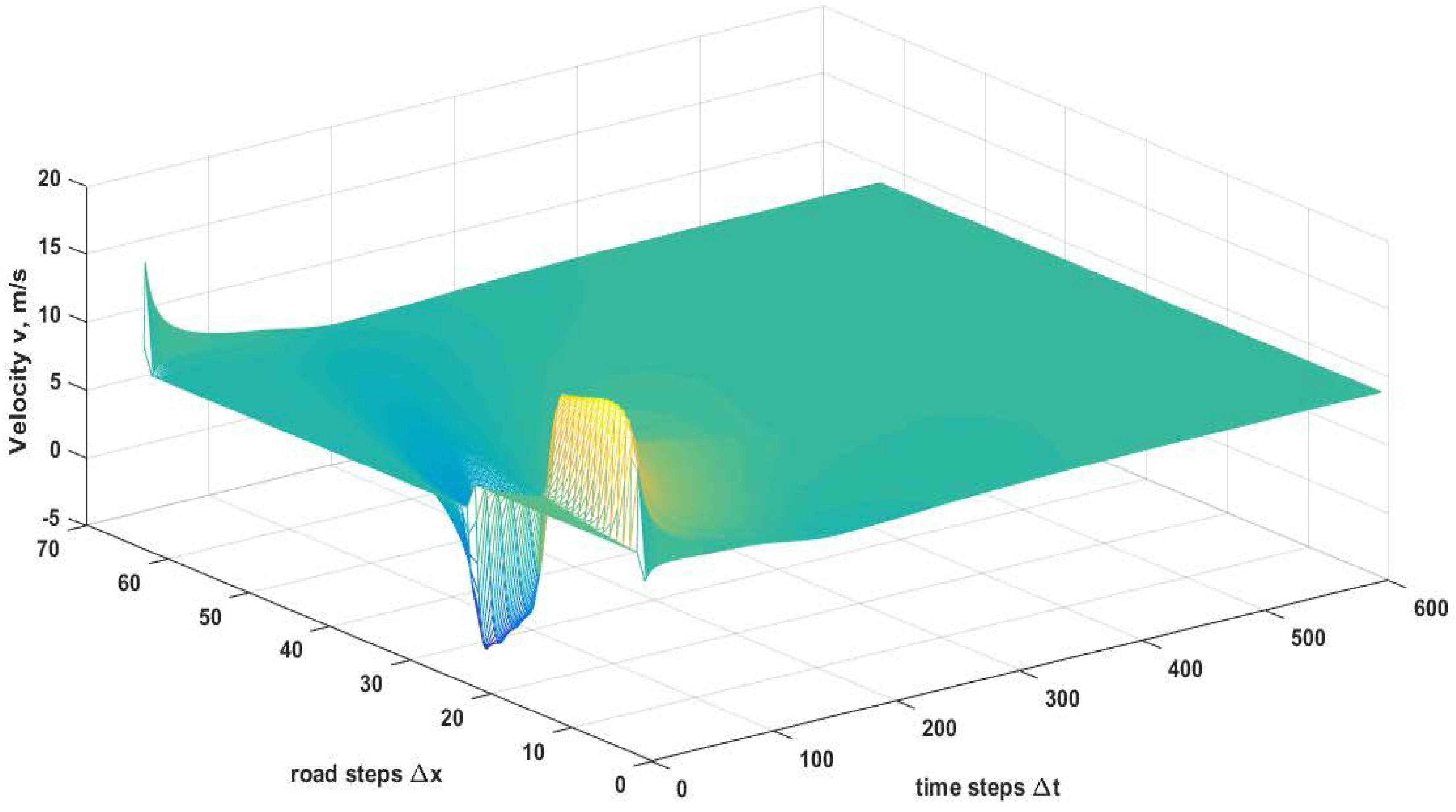
The spatial and temporal density evolution with the proposed model during congestion given by Equation (74) (the density is above the critical density $0.5$ between 130 m and 180 m), for 60 s over the 300 m road is shown in Figure 7. These results show that the density still evolves smoothly over time. The normalized density with the proposed model stays within the minimum 0 and maximum 1, as required. The maximum density with the proposed model at $0.1$ s is $0.8$ at 131 m. At 60 s, the density is very smooth. The corresponding velocity with the proposed model is given in Figure 8. These results show that the velocity evolves smoothly over time and stays within the maximum of 10 m/s and minimum of 0 m/s. At $0.1$ s, the velocity is $0.5$ m/s at 131 m when the density is $0.8$. With the PW model, the velocity is as high as $19.6$ m/s and below 0 m/s, as shown in Figure 6. Thus, the proposed model provides more realistic behavior than the PW model.

The density behavior with the proposed model for time step $0.01$ s and road step 2 m over the 300 m road at 1 s, 20 s, 40 s and 60 s is shown in Figure 9 and given in

Table 5. Velocity and density of the proposed model for the resolution test at 1 s, 20 s, 40 s and 60 s.

Time (s)	Distance (m)	Normalized Density	Velocity (m/s)
1	1	$0.20$	$8.0$
1	28–102	$0.10$	$9.9$
1	118–300	$0.20$	$8.0$
20	1	$0.20$	$8.0$
20	234	$0.01$	$9.9$
20	300	$0.20$	$8.0$
40	1	$0.12$	$8.8$
40	96	$0.02$	$9.7$
40	142	$0.20$	$8.0$
40	300	$0.12$	$8.8$
60	1	$0.20$	$8.0$
60	250	$0.05$	$9.5$
60	260	$0.06$	$9.4$
60	288	$0.19$	$8.1$
60	300	$0.20$	$8.0$

. Comparing the results from 1 s to 60 s, the density becomes smoother over time. At 1 s, the density is $0.20$ at 1 m, and from 28 m to 102 m it is $0.01$. It increases to $0.2$ at 118 m and stays at this level to 300 m. At 20 s, the density is $0.20$ at 1 m, and decreases to $0.01$ at 234 m, and then increases to $0.20$ at 300 m. At 40 s, the density is $0.12$ at 1 m, decreases to $0.02$ at 96 m, and is $0.2$ at 142 m. It is $0.12$ at 300 m. At 60 s, the density is $0.20$ at 1 m and decreases to $0.05$ at 250 m. From 260 m and 288 m, the density varies between $0.06$ and $0.19$ and is $0.20$ at 300 m. The density is smoother at density discontinuities than the results in Figure 1 for time step $0.1$ s and road step 1 m, however there are no significant differences. Thus, the numerical scheme is stable.

The velocity behavior with the proposed model for time step $0.01$ s and road step 2 m over the 300 m road at 1 s, 20 s, 40 s and 60 s is shown in Figure 10 and given in Table 5. At 1 s, the velocity is $8.0$ m/s at 1 m and increases to $9.9$ m/s at 28 m. The velocity is a constant $8.0$ m/s between 118 m and 300 m. At 20 s, the velocity is $8.0$ m/s at 1 m and increases to $9.9$ m/s at 234 m. It is $8.0$ m/s at 300 m. At 40 s, the velocity increases from $8.8$ m/s at 1 m to $9.7$ m/s at 96 m. The velocity is $8.0$ m/s at 142 m, then increases to $8.8$ m/s at 300 m. At 60 s, the velocity is $8.0$ m/s at 1 m and smoothly increases to $9.5$ m/s at 250 m. The velocity varies between $9.4$ m/s and $8.06$ m/s from 260 m to 288 m. It is $8.0$ m/s at 300 m. The velocity behavior of the proposed model with time step $0.01$ s and road step 2 m is smoother at abrupt changes than the results in Figure 2 for time step $0.1$ s and road step 1 m. However, there are no significant differences, which confirms that the numerical scheme is stable.

6. Conclusions

A new macroscopic traffic flow model was proposed. The velocity and density with this model were shown to remain within limits with no oscillations. Conversely, the Payne–Whitham (PW) model results in unrealistic behavior due to the use of a speed constant $C_0$. The PW model spatial density adjustments are based only on this constant regardless of the stimuli. This results in negative velocities as well as the velocities above the maximum, which is impossible. In the proposed model, these changes in density are based on driver reaction and traffic stimuli. As a consequence, the results obtained are more realistic than with the PW model.