Study on Low-Speed Stability of a Motorcycle

Abstract

The increased number of vehicles and poor road conditions in many countries result in slow moving traffic. At low-speeds, riding a motorcycle requires continuous input from a rider to achieve stability, which causes fatigue to the rider. Therefore, in this research, the low-speed stability of a motorcycle is studied using a theoretical and experimental approach to identify the parameters that can reduce the rider’s effort. Initially, a linear mathematical model of the motorcycle and rider system is presented; wherein, the equation of motion for the stability of the system in roll direction is derived. The open-loop and closed-loop poles from the equation are calculated to determine the regions for the low-speed stability. Subsequently, experiments are conducted on the motorcycle instrumented with the required sensors, on a straight path at speeds below 10 km/h. The input and output parameters from the experimental data are analyzed using a statistical method. Steering angle and steering torque are the input parameters; roll and yaw angles and their corresponding velocities are the output parameters selected for the analysis. Correlation and lead time between the input and output parameters are compared to identify the parameters useful for the rider to attain the low-speed stability. The results obtained from the experimental analysis validate the mathematical model. In addition, these findings also validate that the input parameters required to control the motorcycle to achieve low-speed stability can be estimated using the identified output parameters.

1. Introduction

Motorcycles are a preferred mode of daily transportation in many countries because of congested traffic conditions, and also they are the most economically viable option. The traffic congestion and poor road conditions constrain the speed of motorcycles. Balancing a motorcycle at low-speeds is challenging, especially for new riders because it is unstable below the certain critical speed [1,2]. The rider becomes very cautious at such speeds as it requires continuous input to balance the motorcycle [3]; moreover, the required steering input or the gain value for the steering input increases as speed reduces [4]. This research focuses on the low-speed stability of the motorcycle due to the above-mentioned reasons.

The layout of a motorcycle influences its stability [5,6,7]. However, it cannot be tuned entirely for stability because it also determines other performance requirements such as manoeuvrability, ride comfort, ergonomics, acceleration feel, braking, etc. Hence, it is necessary to explore other methods to improve stability. In research [8,9,10], the relations between input and output parameters of a motorcycle are examined to construct a rider robot. Wherein, the speeds are relatively higher, and inputs are derived from the control engineering requirements. Similarly, in research studies [11,12], the low-speed stability of a bicycle is proposed using a theoretical approach. In such cases, frequencies of input to the bicycle are different from that provided by the riders.

The steering input required to improve the low-speed stability can be reduced by adding an extra degree of freedom to a motorcycle using a mechanism [13]. The low-speed stability of a bicycle or motorcycle can also be achieved by adding a device that provides gyroscopic moments [14,15,16]. In research [17], the low-speed stability of the motorcycle is achieved by providing steering to both front and rear wheels, unlike a typical motorcycle. However, these changes may not retain the conventional form and dynamics of the motorcycle. A small humanoid robot can balance and steer a scaled-down bicycle by providing input to the handlebar, using the lateral dynamics of the bicycle [18]. A mathematical model of the bicycle and motor integrated by a controlled algorithm can reduce the step of estimating the steering angle for balancing it [19]. In research [20], the bicycle is balanced using both, flywheel and balancer; however, the study of system behaviour coupled with the steering input by the rider is undone. In research [21], the bicycle is balanced by controlling its steering, using the dynamic model derived from the equilibrium of gravity and centrifugal force. In these research studies, the balancing of the bicycle or the motorcycle is attained without assessing the inputs from an actual rider. Whereas, in the present study, the stability of the motorcycle at low-speeds is studied using experiments by the actual riders.

There are many research studies on improving and assessing the stability (weave and wobble) and handling characteristics of the motorcycle at high speeds [22,23,24]. Whereas, there are limited studies on low-speeds stability of motorcycle by evaluating the rider inputs [25,26], which is the scope of the present research.

In this research, the low-speed stability of a scooter-type motorcycle is studied using theoretical and experimental methods. The details of the motorcycle and the research methodology are given in Section 2. Equation of motion for the theoretical model of the motorcycle is presented in Section 3; wherein, the regions of stability of the motorcycle at speeds 3 and 5 km/h are shown. The experiments and method of analysis are discussed in Section 4. In this section, the theoretical model of the motorcycle is validated, and the parameters important for the low-speed stability are identified and evaluated. The conclusions of the research are given in Section 5.

2. Experimental Motorcycle and Methodology

2.1. Motorcycle Details

The layout, mass and inertia of a scooter-type motorcycle chosen for this research are provided in

Table 1. Layout, mass and inertia of the motorcycle including a rider weighing 65 kg.

Parameters	Symbols	Values	Unit
Total mass	M	165.70	kg
Wheelbase	l	1.236	m
Roll inertia at centre of gravity	$I_g$	18.79	${\mathrm{kgm}}^2$
Height of centre of gravity from ground	h	0.545	m
Horizontal distance of centre of gravity from rear axle	$l_r$	0.450	m
Caster angle	$ϵ$	25.8	degree
Fork offset	$d_1$	0.004	m
Front steering system mass	$M_f$	17.72	kg
Height of front steering system centre of gravity from ground	$h_f$	0.540	m
Shortest distance between steering system centre of gravity and steering axis	d	0.005	m
Front wheel rolling radius	$r_f$	0.214	m
Front wheel spin inertia	$I_{fw}$	0.122	${\mathrm{kgm}}^2$
Rear wheel rolling radius	$r_r$	0.205	m
Rear wheel spin inertia	$I_{rw}$	0.112	${\mathrm{kgm}}^2$
Acceleration of gravity	g	9.81	${\mathrm{m}/\sec }^2$

. The same table also shows the symbols corresponding to the parameters used in this paper.

The motorcycle-rider system used for studying low-speed stability is shown in Figure 1. The figure shows that the rider estimates the required input using the state feedback of the motorcycle. The disturbances; road irregularities and rider disruptions shown in the model are components of the output and the input parameters respectively. In general, any disturbance to the motorcycle affects its output parameters which in turn results in a change in the rider input. The objective of the rider is to keep the motorcycle stable by maintaining the reference value of the output parameters (i.e., roll angle ($\varphi$) to be zero in this case).

2.2. Methodology

In this research, the stability of the motorcycle at low-speed is studied using theoretical and experimental methods. At first, the equations for open-loop and closed-loop systems of the motorcycle were derived for the stability in roll direction using a linear motorcycle model. The regions of stability were determined by solving the equations. Subsequently, experiments were conducted on an actual motorcycle. The motorcycle was ridden on a straight path at speeds ranging from 3 to 10 km/h by professional riders, having riding experience of more than 15 years. The input and output parameters of the motorcycle from the experiments were analyzed using a statistical method. The correlation and lead time between the input and the output parameters were compared to identify the parameters contributing to the low-speed stability. Results obtained from the experiments validated the theoretical model and also confirm that the identified input parameter required to balance the motorcycle at low speeds can be estimated accurately using the identified output parameters.

3. Linear Motorcycle Model

A linear mathematical model for the motorcycle is described in this section. An equation of motion for the stability of the motorcycle is determined in the roll direction. Open-loop and closed-loop systems for the motorcycle are defined using the same equation. In this model, it is assumed that the tire thickness is zero, and all the angles are small.

The layout of a typical motorcycle is shown in Figure 2. The descriptions of the symbols used in the figure are given in Table 1 from Section 2. The points A and O are contact points of the front and rear wheels with ground respectively, and B is the point where the steering axis intersects the ground.

Figure 3 depicts the schematic of the motorcycle, which shows its different states while balancing. The symbols used in the figure are listed in

Table 2. Input and output parameters used in linear model.

Parameters	Symbols
Roll angle	$\varphi$
Steering angle	$\delta$
Kinematic steering angle	${\delta }_R$
Yaw angle	$\psi$
Lateral displacement at O	$y_o$
Speed	v
Instantaneous turning circle radius	R

. The figure shows that the motorcycle-rider system (mass M) first steered by an angle ($\delta$) as shown by legend 2, and then rotated about the x-axis by a roll angle ($\varphi$) as shown by legend 3. These steering angle and roll angle are generated due to disturbances to the motorcycle. Figure 3a,b show rear-view and top-view of the motorcycle respectively. Various forces acting on the motorcycle are due to weight ($Mg$), normal reaction (N) and lateral force ($F_y$) as shown in the Figure 3a. The Figure 3b shows the effect of steering angle ($\delta$) and roll angle ($\varphi$) on the motorcycle state. Marginal changes in $\delta$ and $\varphi$, which result in yaw angle ($\psi$), make the motorcycle to follow a circle of radius R. The significance of the steering mechanism on the stability of the motorcycle is described in this section.

The equation of motion for the stability of the motorcycle in roll direction about the x-axis (i.e., the axis intersecting vehicle plane and ground plane at point O) is defined as follows:

$$I_o\ddot{\varphi }+M{\ddot{y}}_{o}h=Mgh\varphi +M_{gyro}+M_{steering}+M_{frontnormalreaction},$$

(1)

where:

The inertia of the motorcycle with respect to point O is as follows:

$$I_o=I_g+M{h}^2.$$

(2)

The lateral acceleration of the motorcycle $\ddot{y}$ about point O is a function of the centrifugal force and lateral velocity. These parameters are derived from motorcycle speed v and kinematic steering angle ${\delta }_R$ as shown below:

$${\ddot{y}}_o=\frac{v^2}{l}{\delta }_R+v\frac{l_r}{l}{\dot{\delta }}_R.$$

(3)

Gyroscopic moments by both front and rear wheels on the motorcycle, and by the front wheel on the front steering system can be described as:

$$M_{gyro}=-\frac{v^2}{l}\left(\frac{I_{fw}}{r_f}+\frac{I_{rw}}{r_r}\right){\delta }_R-\frac{v}{r_f}{I}_{fw}{\dot{\delta }}_R.$$

(4)

Moment due to the front steering system vibration is as follows:

$$M_{steering}=-M_{f}d{h}_f\ddot{\delta }.$$

(5)

Moment due to the front wheel normal reaction force is as follows:

$$M_{frontnormalreaction}=Mg\frac{l_r}{l}{d}_1\delta .$$

(6)

The following equation is achieved by substituting the values from Equations (2)–(6) in Equation (1).

$$\begin{array}{c}(I_g+M{h}^2)\ddot{\varphi }+M\left(\frac{v^2}{l}{\delta }_R+v\frac{l_r}{l}{\dot{\delta }}_R\right)h=\hfill \\ Mgh\varphi -\frac{v^2}{l}\left(\frac{I_{fw}}{r_f}+\frac{I_{rw}}{r_r}\right){\delta }_R-\frac{v}{r_f}{I}_{fw}{\dot{\delta }}_R-M_{f}d{h}_f\ddot{\delta }+Mg\frac{l_r}{l}{d}_1\delta .\hfill \end{array}$$

(7)

Further, the kinematic steering angle can be defined by the following equation:

$${\delta }_R={\tan }^{-1}\left(\frac{cos(ϵ)sin(\delta )}{cos(\varphi )cos(\delta )-sin(\varphi )sin(ϵ)sin(\delta )}\right).$$

(8)

Equation (8) can be approximated in linear form as follows:

$${\delta }_R\approx \delta cos(ϵ).$$

(9)

Substituting the value of kinematic steering angle from Equation (9) in Equation (7) gives the following expression:

$$\begin{array}{c}(I_g+M{h}^2)\ddot{\varphi }-Mgh\varphi =\hfill \\ -M\left(\frac{v^2}{l}\delta +v\frac{l_r}{l}\dot{\delta }\right)cos(ϵ)h-\frac{v^2}{l}\left(\frac{I_{fw}}{r_f}+\frac{I_{rw}}{r_r}\right)cos(ϵ)\delta -\frac{v}{r_f}{I}_{fw}cos(ϵ)\dot{\delta }-M_{f}d{h}_f\ddot{\delta }+Mg\frac{l_r}{l}{d}_1\delta .\hfill \end{array}$$

(10)

The open-loop transfer function for the low-speed stability of the motorcycle system can be described from Equation (10) by the following expression:

Open-loop transfer function =

$$\frac{\varphi (s)}{\delta (s)}=\frac{-M\left(\frac{v^2}{l}+v\frac{l_r}{l}s\right)cos(ϵ)h-\frac{v^2}{l}\left(\frac{I_{fw}}{r_f}+\frac{I_{rw}}{r_r}\right)cos(ϵ)-\frac{v}{r_f}{I}_{fw}cos(ϵ)s-M_{f}d{h}_f{s}^2+Mg\frac{l_r}{l}{d}_1}{(I_g+M{h}^2)s^2-Mgh}.$$

(11)

The transfer function defines the stability of the motorcycle at all the speeds.

Root-locus plot for Equation (11) is shown in Figure 4. The figure shows that one of the poles of the system is always positive at speeds 3, 5 and 10 km/h. Hence, the low-speed stability for the open-loop system of the motorcycle cannot be achieved.

Further, the closed-loop feedback of the motorcycle can be defined using the following relationship between the steering angle ($\delta$) and roll angle ($\varphi$):

$$\delta (t)=a.\varphi (t-\tau ),$$

(12)

where a is roll angle gain and $\tau$ is a lead time for roll angle with respect to the steering angle. Equation (12) can be further simplified for $\tau <1$ as follows:

$$\delta =a.\varphi -a\tau \dot{\varphi }.$$

(13)

Substituting the value from Equation (13) in the Equation (10) following equation is obtained:

$$C_1\stackrel{⃛}{\varphi }+C_2\ddot{\varphi }+C_3\dot{\varphi }+C_4\varphi =0,$$

(14)

where,

$$C_1=-M_f{h}_{f}da\tau$$

(15)

$$C_2=M{h}^2-\frac{Mh{l}_{r}vcos(ϵ)a\tau }{l}+I_g+M_f{h}_{f}da-\frac{I_{fw}vcos(ϵ)a\tau }{r_f}$$

(16)

$$C_3=Mhvcos(ϵ)a\left(\frac{l_r}{l}-\frac{v\tau }{l}\right)+\frac{I_{fw}vcos(ϵ)a}{r_f}-\frac{v^{2}cos(ϵ)a\tau }{l}\left(\frac{I_{fw}}{r_f}+\frac{I_{rw}}{r_r}\right)+\frac{Mg{l}_r{d}_{1}a\tau }{l}$$

(17)

$$C_4=\frac{v^{2}cos(ϵ)a}{l}\left(\frac{I_{f}w}{r_f}+\frac{I_{r}w}{r_r}\right)-Mgh-Ma\left(\frac{gd{l}_r+h{v}^{2}cos(ϵ)}{l}\right).$$

(18)

The constants of the closed-loop characteristic Equation (14): $C_1,C_2,C_3$ and $C_4$ are shown in Equations (15)–(18). The eigenvalues of the characteristic equation are calculated for different values of the roll angle gain a and the lead time $\tau$. The motorcycle is stable at a point where all the real parts of the eigenvalues are negative for a particular value of a and $\tau$. The shaded zones in Figure 5a,b show regions for the stable motorcycle corresponding to the values of a and $\tau$ at speeds 3 and 5 km/h respectively. The rider must be operating inside the shaded zone shown in Figure 5 to achieve the low-speed stability.

In the next section, the theoretical results are validated from experimental results.

4. Experiment and Analysis

4.1. Experiments Details

The motorcycle was instrumented with two analogue sensors namely a potentiometer (range of linearity ±50°) and a piezoelectric sensor (range ±200 Nm and sensitivity −175 pC/Nm) to measure the steering angle and the steering torque respectively. An inertia measurement unit (IMU) (angular rate range ±400°/s with an angle measurement accuracy of 0.2°) was used for measuring roll, pitch and yaw angles, corresponding velocities and accelerations. A GPS antenna was used for measuring longitudinal displacement, lateral displacement and speed of the motorcycle. The data was logged at a sample rate of 100 Hz [27].

The sensors were mounted on the motorcycle for the experiments. The rotating shaft of the potentiometer was mounted on top of the handlebar, and its non-rotating body was fixed to the frame. The handlebar and front steering system were disintegrated, and two flanges were fixed to them such that the faces of the flanges are perpendicular to the steering axis. The piezoelectric sensor was mounted between these flanges under high preload. The IMU was mounted on top of the pillion seat, and the GPS antenna was kept on a metal plate fixed to the rear frame of the motorcycle at the highest point on the motorcycle.

Experiments were conducted on a proving ground using the motorcycle instrumented with aforementioned sensors at speeds 3, 5 and 10 km/h. The motorcycle was ridden on the same dry asphalt road to inhibit the road variations in the results. The riders had instructed to follow a straight line marked on the proving ground. The experiments were conducted mainly to focus on balancing the motorcycle. Three professional riders, having riding experience of more than 15 years, were selected for the experiments to ensure the quality of results. Each rider had repeated the experiments two times to ensure the repeatability of the results.

4.2. Analysis of Experiments

The maximum correlation coefficient (MCC) and the lead time between the input and the output parameters are calculated from the experimental data. Steering angle and steering torque are the input parameters; roll and yaw angles and their corresponding velocities are the output parameters selected for the analysis. The MCC defined herein as a cost function to determine the maximum possible correlation between the input and the output parameters by shifting the output parameter with respect to the input parameter. The time step at which the cost function becomes maximum was defined as the lead time. The MCC is a measure of the dependency of the input parameter on the output parameter, and the lead time indicated the usability of the output parameter by the rider for predicting the steering control.

For example, Figure 6 shows time series data for roll angle and steering angle of a professional rider, normalized in [−1,1] range. The correlation between the roll angle and the steering angle was calculated while shifting the roll angle curve in the time domain at a step size of 0.01 s in the direction as shown by the arrow in the figure. Maximum correlation was observed after shifting the roll angle curve by 0.53 s. This correlation was named as the MCC and the time by which the roll angle was shifted to arrive at it is the lead time (i.e., 0.53 s). The MCC and the lead time are determined from the experimental data for all the riders.

In this research, the experimental data were analyzed using a statistical method. All the experimental data were divided into the sample size of 300 (i.e., 3 s) to examine the instantaneous input and output parameters while balancing the motorcycle at low speeds. The average (avg) and standard deviation (SD) from the experimental data were calculated and compared to ensure the repeatability and reliability of the experiments.

The analysis was done in four stages. Firstly, the repeatability and reliability of the experiments were determined. Secondly, the theoretical results were validated with the experimental results using the relationship between the steering angle and the roll parameters in Equations (12) and (13). Thirdly, the MCC and the lead time were calculated for output parameters with the input parameters. These were calculated to identify the output parameters important for the low-speed stability. Steering angle and steering torque were the input parameters; roll and yaw angles and their corresponding velocities were the output parameters selected for the analysis. Finally, multiple regression analysis (MRA) was performed between the identified output parameters as independent variables and the input parameters as dependent variables, to estimate and identify the most important input parameter between the steering angle and the steering torque. Further, the estimated input parameter from MRA was validated by comparing the same with the measured data.

4.2.1. Repeatability and Reliability of Experiments

Table 3. Averages and standard deviations of motorcycle speed (v) and roll angle gain (a).

Target Speed		3 km/h				5 km/h				10 km/h
		Speed		RA Gain		Speed		RA Gain		Speed		RA Gain
Rider	Set	avg	SD	avg	SD	avg	SD	avg	SD	avg	SD	avg	SD
1	1	2.46	0.32	14.49	4.26	5.54	0.44	6.21	1.34	10.16	0.34	2.59	0.67
1	2	2.56	0.48	14.18	4.20	5.49	0.63	6.55	1.72	10.32	0.35	2.42	0.66
2	1	3.12	0.34	16.31	4.11	5.69	0.71	7.00	1.73	10.62	0.52	2.22	0.50
2	2	2.95	0.40	17.42	5.31	5.81	0.36	7.52	1.44	10.48	0.40	2.63	0.54
3	1	3.12	0.46	9.20	3.92	5.27	0.79	6.46	1.58	11.07	0.59	1.88	0.66
3	2	3.02	0.38	10.78	4.02	5.60	0.57	5.22	1.10	10.36	0.35	2.22	0.51

shows the avg and SD for both the motorcycle speed (v) and roll angle gain (RA gain a, for the positive value regions) for each experiment. The avg and SD were calculated for three professional riders who have ridden the motorcycle at target speeds of 3, 5 and 10 km/h. Each rider repeated the experiments two times (named as ‘set’ in the table). The table shows that the avg and SD of the motorcycle speeds and the roll angle gains match closely when the same rider repeated the experiment. This ensures the repeatability of the experiments.

The avg and SD of the RA gain increased sharply when the target speed reduced from 5 to 3 km/h than the same from 10 to 5 km/h; although, the SD of the speeds were similar. This was due to the fact that the effort and correction in steering input required to attain the low-speed stability increase sharply as speed reduces. The avg and SD in the RA gains were similar for all the rider at the particular target speed, which ensured the reliability of the experiments.

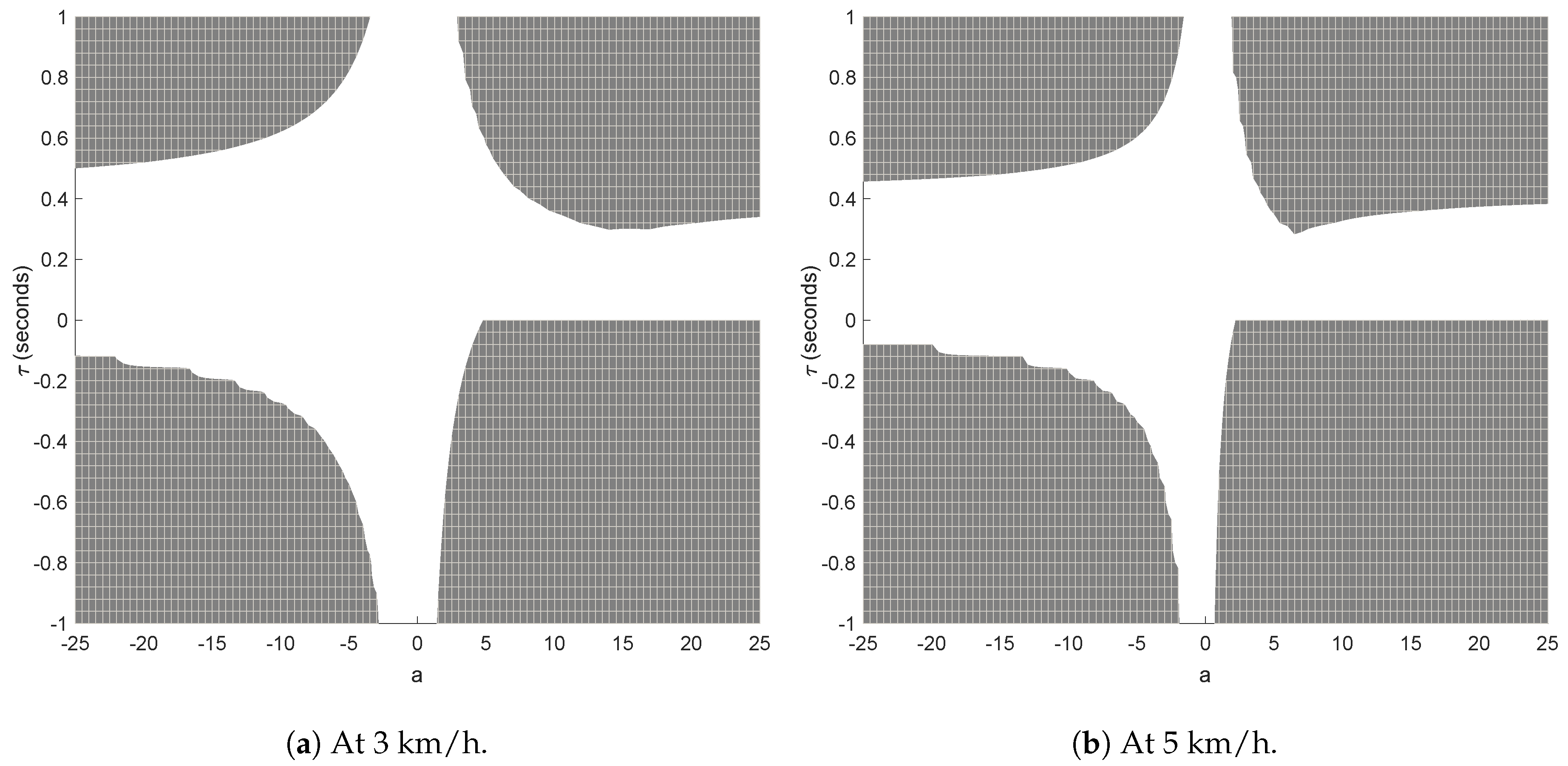
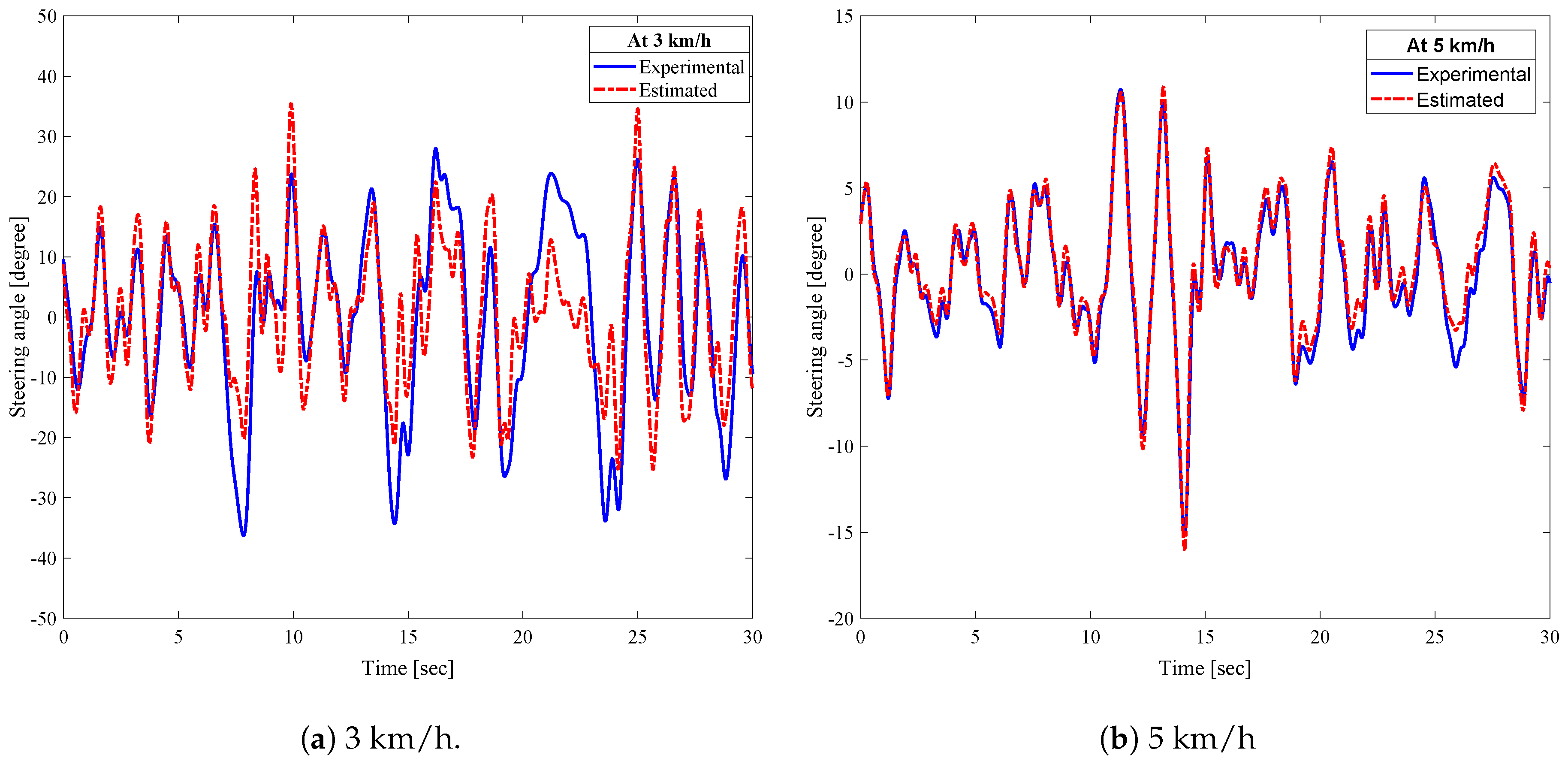
4.2.2. Validation of Theoretical Model

The roll angle gains a and the lead time $\tau$ were calculated as per Equation (12) from the experimental data. The results obtained from the experiments were compared with the theoretical results at speeds 3 and 5 km/h as shown in Figure 7a,b respectively. The figures show that the values of a and $\tau$ calculated from the experiments are in the stable regions determined from the theoretical results thereby validating the theoretical model. It also confirms that the model can be used to predict the stable zone for a motorcycle at low speeds.

Further, the relationship between the steering angle and roll parameters defined by Equation (13) in the Section 3 was examined. Linear MRA between the steering angle as a dependent variable; and, the roll angle and the roll rate as independent variables was performed from the experimental data using the following equation:

$$\delta =a_1\varphi +a_2\dot{\varphi },$$

(19)

where $a_1$ and $a_2$ are the regression coefficients of the roll angle and the roll rate respectively. The regression coefficient $a_2$ was compared with the corresponding coefficient ($-a\tau$) of roll rate derived from the experimental data as per the Equation (13). The correlation coefficients between the coefficients $a_2$ and ($-a\tau$) were strong and more than 0.7. Figure 8 shows that both the coefficients match closely which shows the strong relationship between the theoretical model and experimental results.

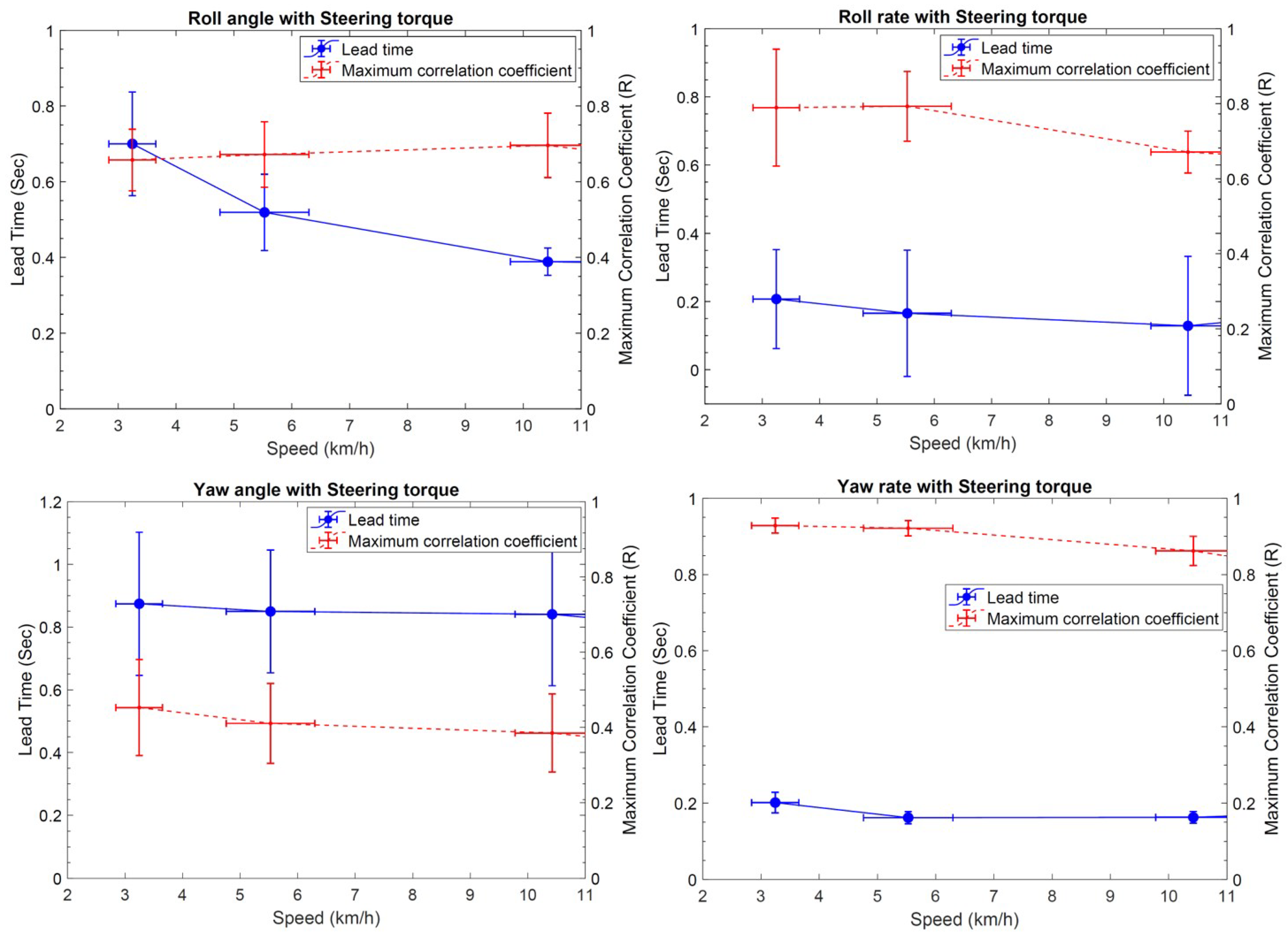
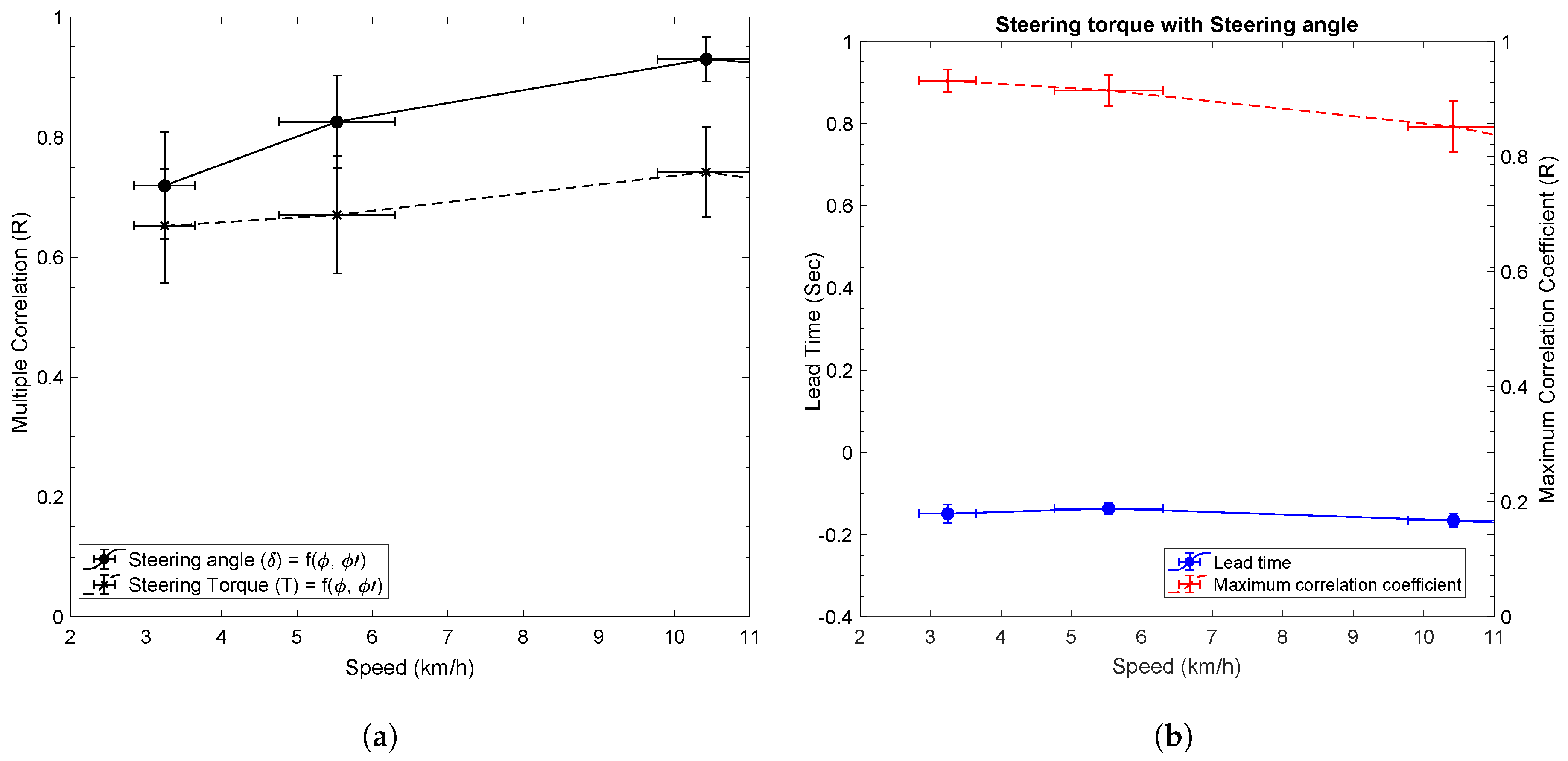
4.2.3. Correlation Analysis

In this section, the experimental data are analyzed to identify the important input and output parameters for the low-speed stability of the motorcycle.

The avg and SD for the lead time and the MCC, for the output parameters with steering angle and steering torque are shown in Figure 9 and Figure 10 respectively using error bars. The MCC is calculated for the leading side of the output parameters such that it can be used for estimating the steering input to achieve the low-speed stability. The results of the analysis are examined in two steps: Firstly, the MCCs between the input and the output parameters are compared to identify the output parameters which can estimate the input parameter. Secondly, the lead time between useful output parameters and input parameters are compared to assess their usability by the riders.

Figure 9 shows that the roll angle and the roll rate are the output parameters that can estimate the steering angle because the MCCs for these parameters with steering angle are strong; and, the lead time is also sufficient to be used by the riders. Whereas, the correlation between the yaw angle and steering angle is weak. The correlation between steering angle and yaw rate was strong (above 0.9) at 3 and 5 km/h. Although, it was not the parameter useful for the riders because its lead time was too low and beyond the human limit to use it for estimating the steering angle.

Similarly, Figure 10 shows that the steering torque can be estimated from roll angle, roll rate and yaw rate because the MCCs between the steering torque and these parameters are strong. Whereas, the MCC between the yaw angle and steering torque was weak. The lead time for the yaw rate with the steering torque is below 0.2 s, which was lower than typical human response time. Thus, the yaw rate cannot be used by the rider for estimating steering torque, and it is a result of the change in other parameters. Therefore, the roll angle and the roll rate are important output parameters used by the riders to estimate the steering input to balance the motorcycle.

Further, the appropriate input parameter between the steering torque and the steering angle is selected based on two requirements. Firstly, the multiple correlations between the input parameter and output parameters i.e., roll angle and roll rate should be strong. Secondly, it is preferred to select the input that can be applied as late as possible to accommodate the delay in the system.

The MRA was performed individually for steering angle and steering torque as a dependent parameter using Equation (19). Figure 11a shows that the regression correlation between the identified output parameters (i.e., the roll angle and the roll rate) and the steering angle was stronger than the same with the steering torque. This shows that the steering angle can be estimated more accurately than the steering torque. The lead time and the MCC for the steering torque with the steering angle are shown in Figure 11b. The MCC between the parameters is strong. The negative lead time (approximately −0.15 s) shows that the steering torque had a delay with respect to the steering angle, which made it a suitable parameter for accommodating the delay in the system. Although, the steering angle was selected as an appropriate input parameter as the priority is given to the accurate estimation of the input parameter from the output parameters.

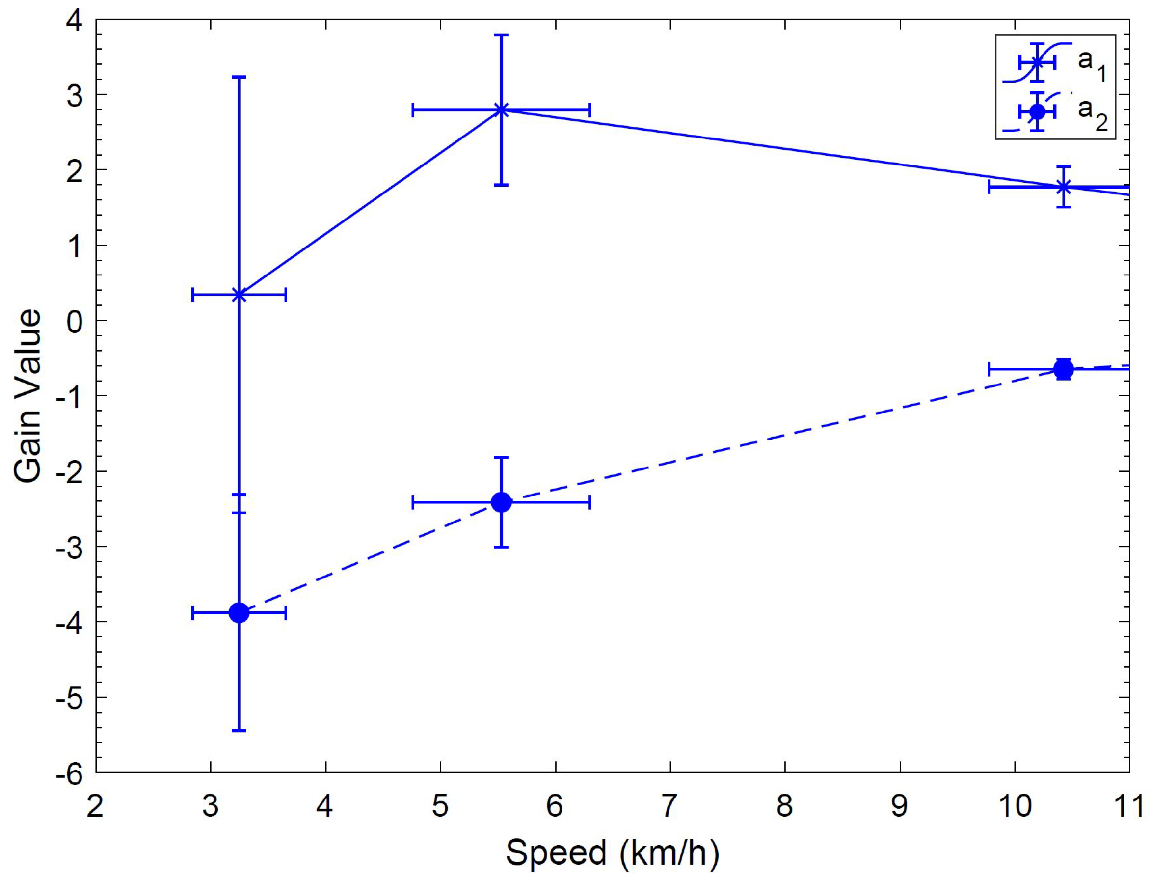
4.2.4. Output Parameter Evaluation

The steering angle was estimated from the roll angle and roll rate using the MRA Equation (19). The mean values of the regression coefficients $a_1$ and $a_2$ are shown in Figure 12, which can be defined by Equations (20) and (21), respectively as a function of motorcycle speed v.

$$a_1=0.011v^3-0.27v^2+2.5v-5$$

(20)

$$a_2=-0.044v^2+0.92v-6.4$$

(21)

The steering angle estimated from the regression model is compared with its measured data from the experiments as shown in Figure 13. Figure 13a,b show that the estimated steering angle matches closely with the measured steering angle at speeds 3 and 5 km/h respectively. These results validate that the regression model can be used for estimating the steering angle, using the roll angle and roll rate accurately.

5. Conclusions

In this research, the low-speed stability of a scooter-type motorcycle is studied using theoretical and experimental methods. The regions for the stability of the motorcycle are determined from the theoretical method. Subsequently, experiments are conducted on a straight path with professional riders at speeds 3, 5 and 10 km/h. A detailed analysis of experimental data is performed using statistical methods. Maximum correlation coefficient and lead time between input and output parameters are calculated and compared to identify the important output parameters to achieve the stability of the motorcycle at low speeds. Further, the appropriate input parameter is identified from a linear multiple regression analysis between the identified output parameters and the input parameters. Following conclusions are drawn from the study:

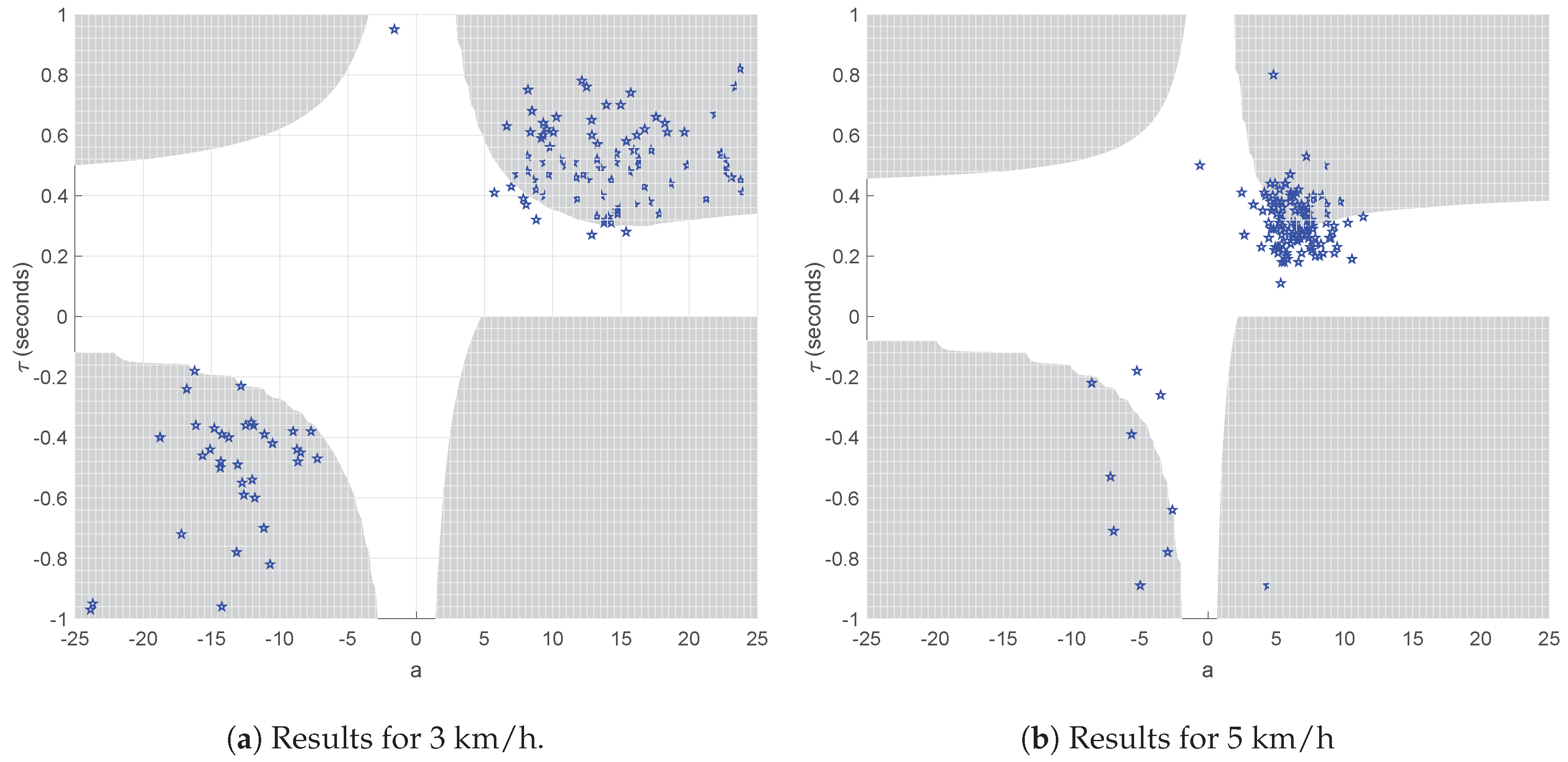
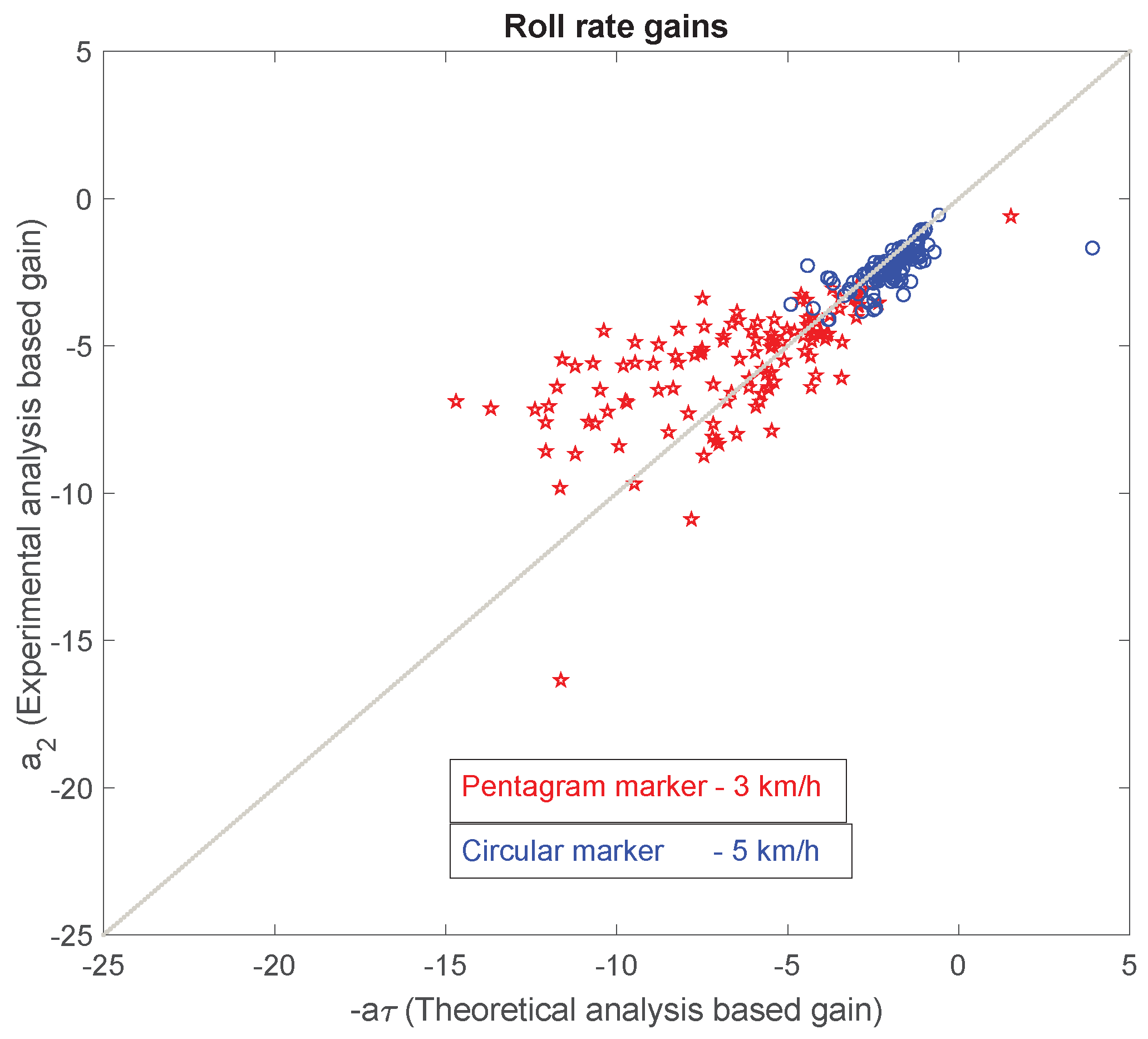
• The experimental results validate that the theoretical method of analysis can be used to find the regions of low-speed stability of a motorcycle.
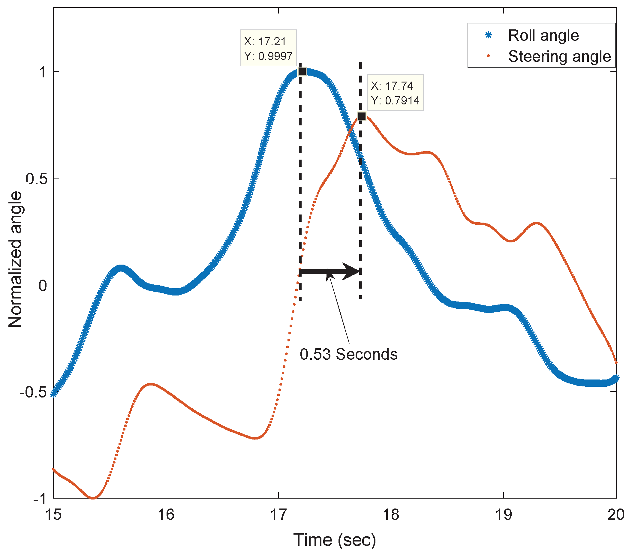
• The roll angle and roll rate are important output parameters to be assessed to achieve low-speed stability.
• The steering angle is the appropriate input parameter over steering torque for low-speed stability because the regression correlation for the steering angle is significantly stronger than the steering torque, with the roll angle and the roll rate.

In future, the results obtained from this research are to be used for developing a controller that can enable a motorcycle in attaining the low-speed stability, which is to be validated by simulations and experiments. Also, the theoretical model is to be improved by including other forces and parameters such as overturning moments, tire thickness and pitch motion of the motorcycle.

References

1. Astrom, K.J.; Klein, R.E.; Lennartsson, A. Bicycle dynamics and control: Adapted bicycles for education and research. IEEE Control Syst. 2005, 25, 26–47. [Google Scholar] [CrossRef]
2. Sharp, R.S. The stability and control of motorcycles. J. Mech. Eng. Sci. 2005, 13, 316–329. [Google Scholar] [CrossRef]
3. Zhang, Y.; Li, J.; Yi, J.; Song, D. Balance control and analysis of stationary riderless motorcycles. In Proceedings of the 2011 IEEE International Conference on Robotics and Automation, Shanghai, China, 9–13 May 2011; pp. 3018–3023. [Google Scholar] [CrossRef]
4. Yokomori, M.; Higuchi, K.; Ooya, T. Rider’s Operation of a Motorcycle Running Straight at Low Speed. JSME Int. J. 1992, 35, 553–559. [Google Scholar] [CrossRef]
5. Kooijman, J.D.G.; Meijaard, J.P.; Papadopoulos, J.M.; Ruina, A.; Schwab, A.L. A Bicycle Can Be Self-Stable Without Gyroscopic or Caster Effects. Sci. Mag. 2005, 332, 339–342. [Google Scholar] [CrossRef] [PubMed]
6. Jones, D.E.H. The stability of the bicycle. Phys. Today 1970, 23, 34–40. [Google Scholar] [CrossRef]
7. Cossalter, V. Motorcycle Dynamics, 2nd ed.; Lulu.com: Morrisville, NC, USA, 2007. [Google Scholar]
8. Miyagishi, S.; Kageyama, I.; Takama, K.; Baba, M.; Uchiyama, H. Study on construction of a rider robot for two-wheeled vehicle. JSAE Rev. 2003, 24, 321–326. [Google Scholar] [CrossRef]
9. Takenouchi, S.; Sekine, T.; Okano, M. Study on condition of stability of motorcycle at low speed. In Proceedings of the Small Engine Technology Conference & Exposition, Kyoto, Japan, 29–31 October 2002; No. 2002-32-1797. SAE Technical Paper: Warrendale, PA, USA, 2002. [Google Scholar]
10. Schlipsing, M.; Salmen, J.; Lattke, B.; Schröter, K.G.; Winner, H. Roll angle estimation for motorcycles: Comparing video and inertial sensor approaches. In Proceedings of the IEEE Intelligent Vehicles Symposium, Alcala de Henares, Spain, 3–7 June 2012; pp. 500–505. [Google Scholar] [CrossRef]
11. Schwab, A.L.; Kooijman, J.D.G.; Meijaard, J.P. Some recent developments in bicycle dynamics and control. In Proceedings of the Fourth European Conference on Structural Control (4ECSC), St. Petersburg, Russia, 8–12 September 2008. [Google Scholar]
12. Zhang, Y.; Yi, J. Dynamic modeling and balance control of human/bicycle systems. In Proceedings of the 2010 IEEE/ASME International Conference on Advanced Intelligent Mechatronics, Montreal, QC, Canada, 6–9 July 2010; pp. 1385–1390. [Google Scholar] [CrossRef]
13. Kimura, T.; Ando, Y.; Tsujii, E. Development of new concept two-wheel steering system for motorcycles. SAE Int. J. Passeng. Cars Electron. Electr. Syst. 2014, 7, 36–40. [Google Scholar] [CrossRef]
14. Beznos, A.V.; Formal’sky, A.M.; Gurfinkel, E.V.; Jicharev, D.N.; Lensky, A.V.; Savitsky, K.V.; Tchesalin, L.S. Control of autonomous motion of two-wheel bicycle with gyroscopic stabilisation. In Proceedings of the 1998 IEEE International Conference on Robotics and Automation, Leuven, Belgium, 16–20 May 1988; Volume 3, pp. 2670–2675. [Google Scholar] [CrossRef]
15. Lot, R.; Fleming, J. Gyroscopic stabilisers for powered two-wheeled vehicles. Veh. Syst. Dyn. 2018. [Google Scholar] [CrossRef]
16. Karnopp, D. Tilt control for gyro-stabilized two-wheeled vehicles. Veh. Syst. Dyn. 2002, 37, 145–156. [Google Scholar] [CrossRef]
17. Yang, C.; Murakami, T. Full-speed range self-balancing electric motorcycles without the handlebar. IEEE Trans. Ind. Electron. 2016, 63, 1911–1922. [Google Scholar] [CrossRef]
18. Huang, C.; Tung, Y.; Yeh, T. Balancing control of a robot bicycle with uncertain center of gravity. In Proceedings of the IEEE International Conference on Robotics and Automation (ICRA), Singapore, 29 May–3 June 2017; pp. 5858–5863. [Google Scholar] [CrossRef]
19. Vatanashevanopakorn, S.; Parnichkun, M. Steering control based balancing of a bicycle robot. In Proceedings of the 2011 IEEE International Conference on Robotics and Biomimetics, Karon Beach, Phuket, Thailand, 7–11 December 2011; pp. 2169–2174. [Google Scholar] [CrossRef]
20. Keo, L.; Yoshino, K.; Kawaguchi, M.; Yamakita, M. Experimental results for stabilizing of a bicycle with a flywheel balancer. In Proceedings of the 2011 IEEE International Conference on Robotics and Automation, Shanghai, China, 9–13 May 2011; pp. 6150–6155. [Google Scholar] [CrossRef]
21. Tanaka, Y.; Murakami, T. Self sustaining bicycle robot with steering controller. In Proceedings of the AMC ‘04 8th IEEE International Workshop on Advanced Motion Control, Kawasaki, Japan, 25–28 March 2004; pp. 193–197. [Google Scholar] [CrossRef]
22. Sharp, R.S.; Watanabe, Y. Chatter vibrations of high-performance motorcycles. Veh. Syst. Dyn. 2013, 51, 393–404. [Google Scholar] [CrossRef]
23. Massaro, M.; Lot, R.; Cossalter, V.; Brendelson, J.; Sadauckas, J. Numerical and experimental investigation of passive rider effects on motorcycle weave. Veh. Syst. Dyn. 2012, 50 (Suppl. 1), 215–227. [Google Scholar] [CrossRef]
24. Sakai, H. Theoretical and Fundamental Consideration to Accord Between Self-Steer Speed and Rolling in Maneuverability of Motorcycles; No. 2018-32-0049; SAE Technical Paper: Warrendale, PA, USA, 2018. [Google Scholar] [CrossRef]
25. Karanam, V.M. Studies in the Dynamics of Two and Three Wheeled Vehicles. Ph.D. Thesis, Indian Institute of Science, Bangalore, India, 2012. [Google Scholar]
26. Popov, A.A.; Rowell, S.; Meijaard, J.P. A review on motorcycle and rider modelling for steering control. Veh. Syst. Dyn. 2010, 48, 775–792. [Google Scholar] [CrossRef]
27. Data Logger. Available online: http://www.racelogic.co.uk/_downloads/vbox/Datasheets/Data_Loggers/RLVB3i_Data.pdf (accessed on 27 April 2019).
Figure 1. Block diagram for the low-speed stability of a motorcycle and rider system.
Applsci 09 02278 g001
Figure 2. A typical layout of a motorcycle.
Applsci 09 02278 g002
Figure 3. Schematic of linear model of motorcycle showing its different states.
Applsci 09 02278 g003
Figure 4. Root-locus plot for open-loop motorcycle system.
Applsci 09 02278 g004
Figure 5. Regions of stability for different values of roll angle gain a and lead time τ for closed-loop system of motorcycle.
Applsci 09 02278 g005
Figure 6. Steering angle and roll angle curve of a rider normalized in [−1,1] range @ 3.1 km/h.
Applsci 09 02278 g006
Figure 7. Validation of theoretical results from experiments.
Applsci 09 02278 g007
Figure 8. Validation of roll rate gain values based on theory and experiments.
Applsci 09 02278 g008
Figure 9. MCC (R) and lead time for output parameters with the steering angle.
Applsci 09 02278 g009
Figure 10. Maximum correlation coefficient (MCC) (R) and lead time for output parameters with steering torque.
Applsci 09 02278 g010
Figure 11. Analyses to select an appropriate input parameter between the steering angle and the steering torque. (a) Regression correlation for the steering angle and the steering torque; (b) Lead time and MCC (R) for the steering torque with the steering angle.
Applsci 09 02278 g011
Figure 12. Regression coefficients for roll angle ( a 1 ) and roll rate ( a 2 ).
Applsci 09 02278 g012
Figure 13. Validation of estimated steering angle from the experimental measurements.
Applsci 09 02278 g013