Dual Stratified Nanofluid Flow Past a Permeable Shrinking/Stretching Sheet Using a Non-Fourier Energy Model

 ,
, 
Abstract
1. Introduction
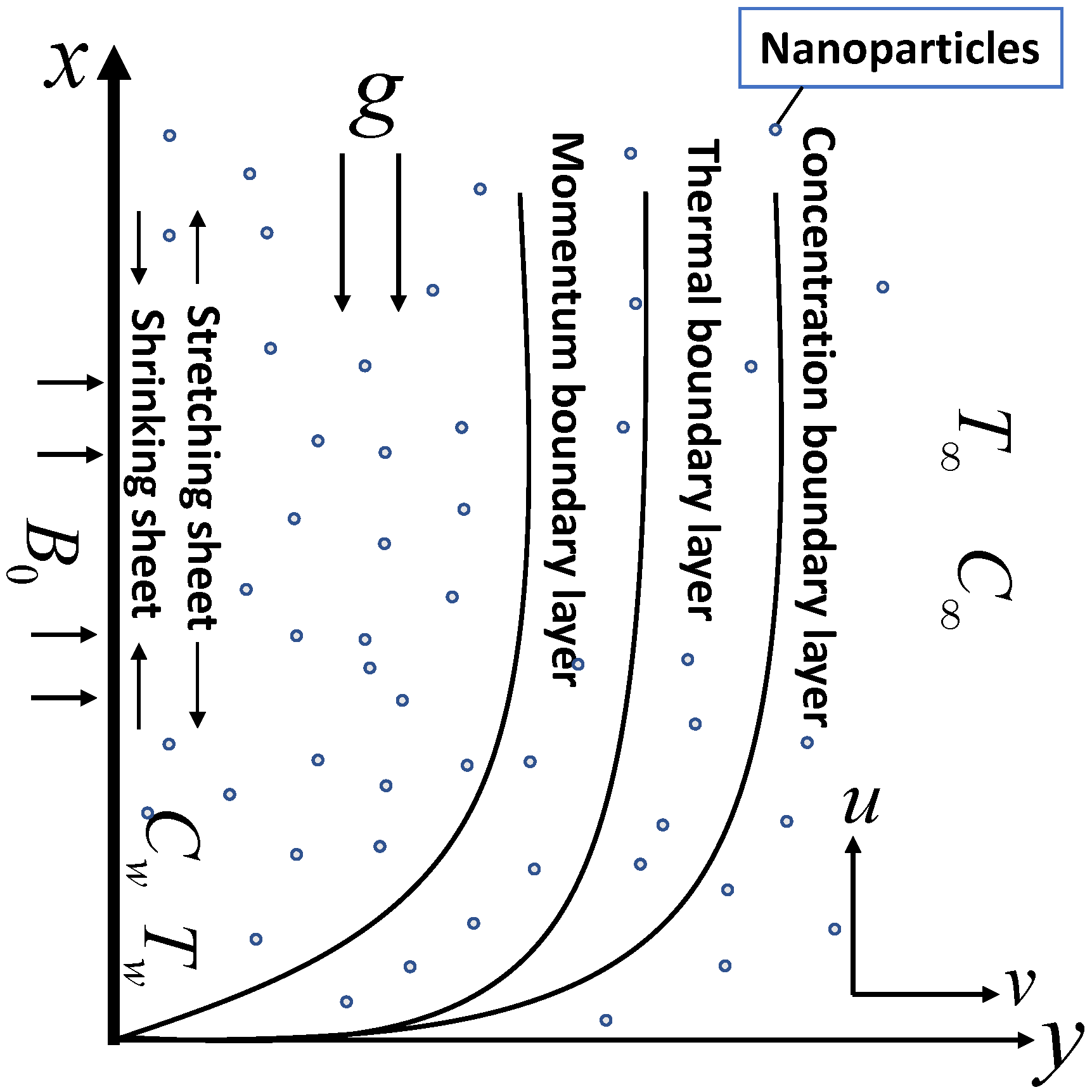
2. Problem Formulation
- The nanoparticles and the base fluid are assumed in a thermal equilibrium state.
- The Buongiorno’s model of nanofluid is used to incorporate the mixed effects of Brownian motion and thermophoresis.
- The induced magnetic field is negligible as a result of the insignificant value of the magnetic Reynolds number
- The Hall current effect is excluded with an assumption of no external electric field is applied to the physical model.
- Thermal and solutal stratifications exist due to the appearance of thermal and solutal buoyancy forces.
2.1. Cattaneo Christov Heat Flux Model
2.2. Steady Flow Formulation
3. Stability Analysis
4. Results and Discussion
5. Conclusions
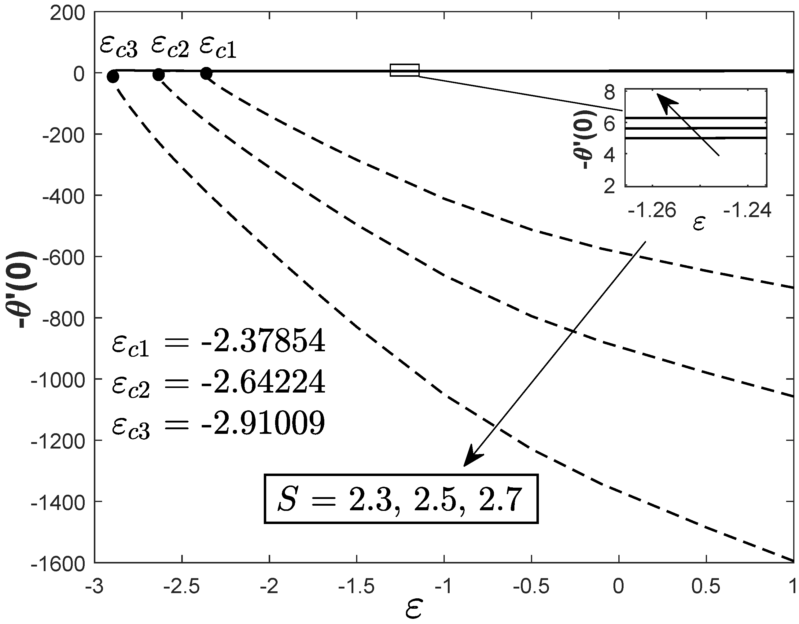
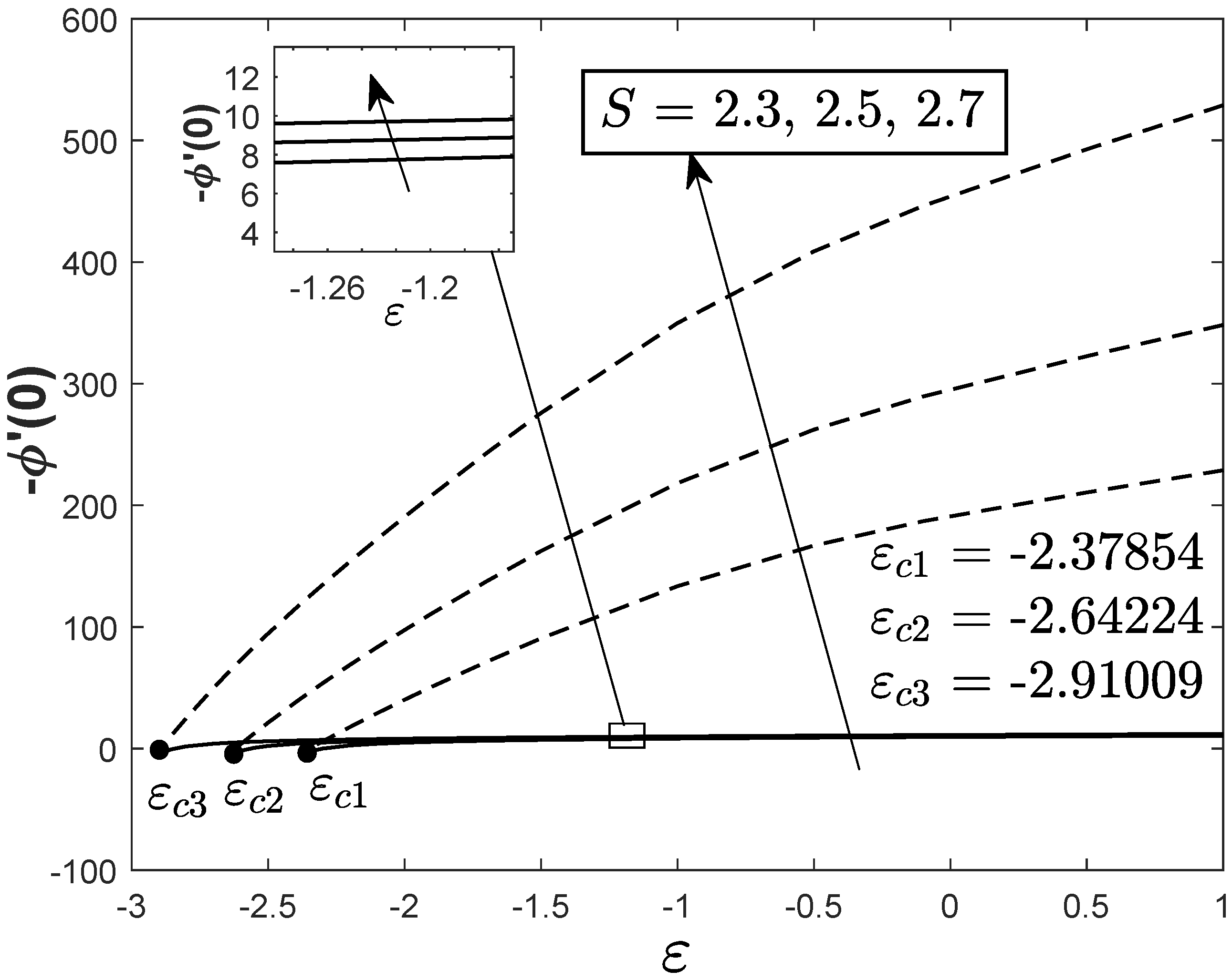
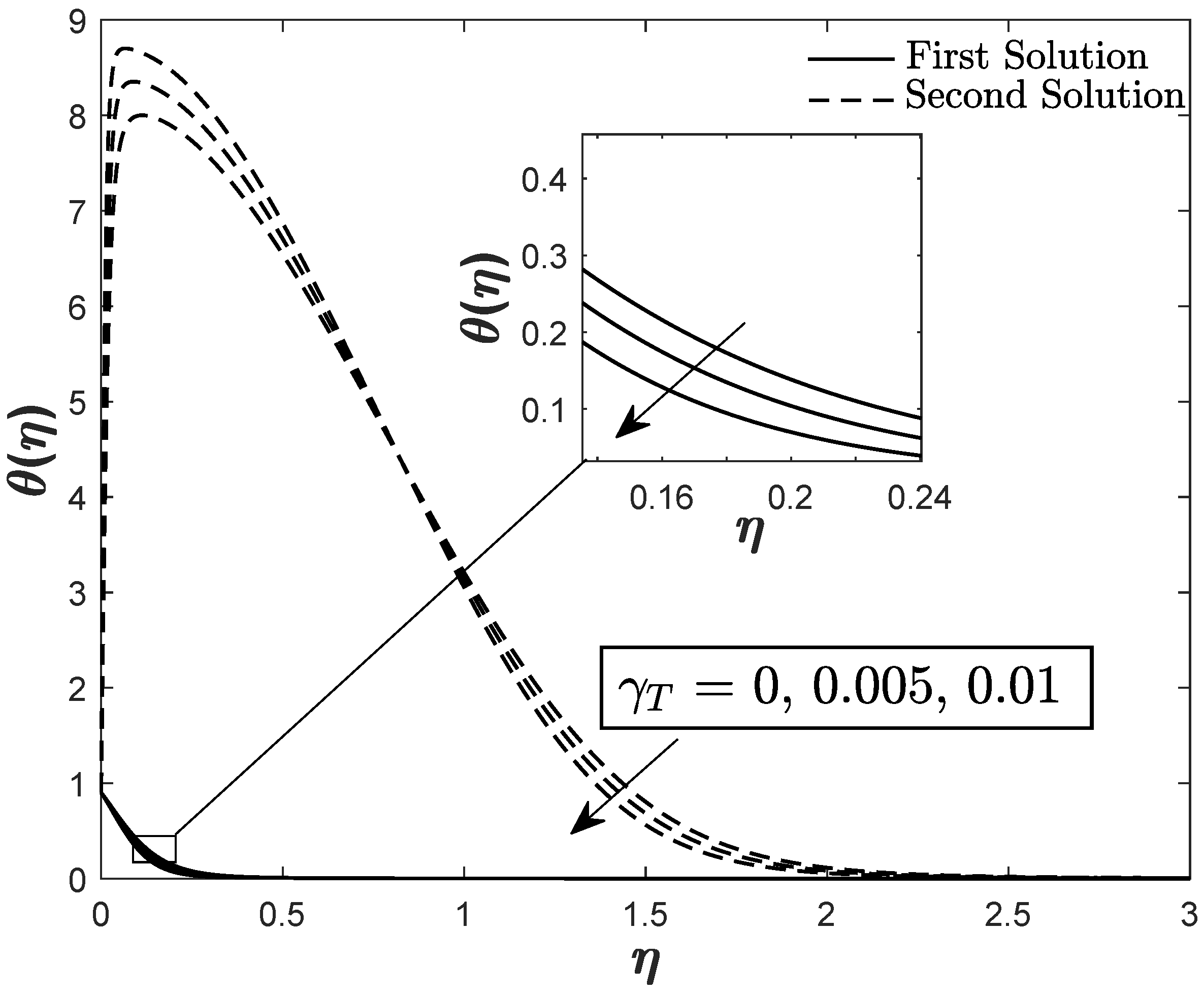
- Thermal relaxation parameter which is resulting from the application of the non-Fourier energy model, gives a different estimation of the heat and mass transfer rates as compared to the classical energy equation. The rate of heat transfer increases whereas the mass transfer rate decreases with the improvement of the thermal relaxation parameter for both stretching and shrinking cases.
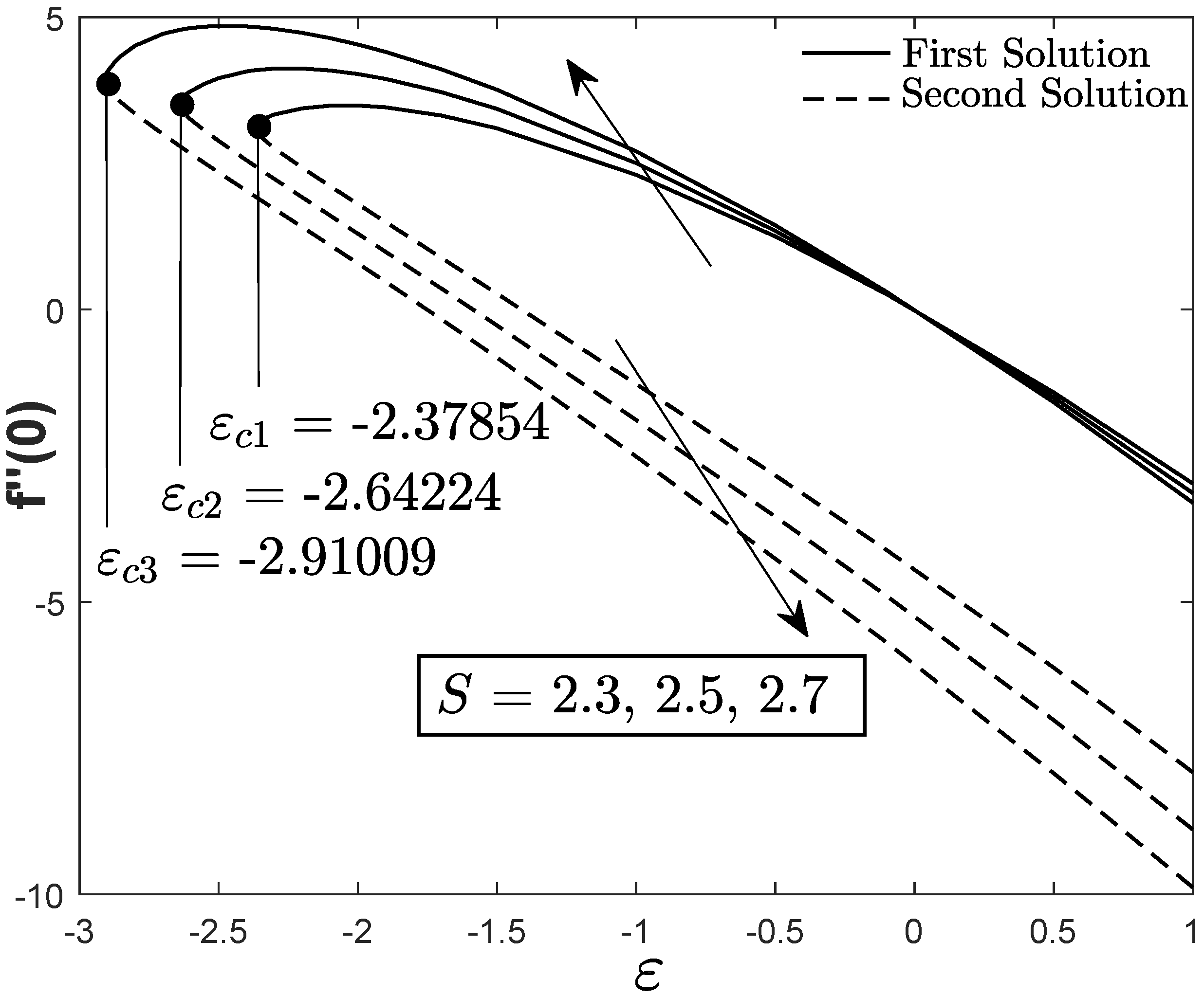
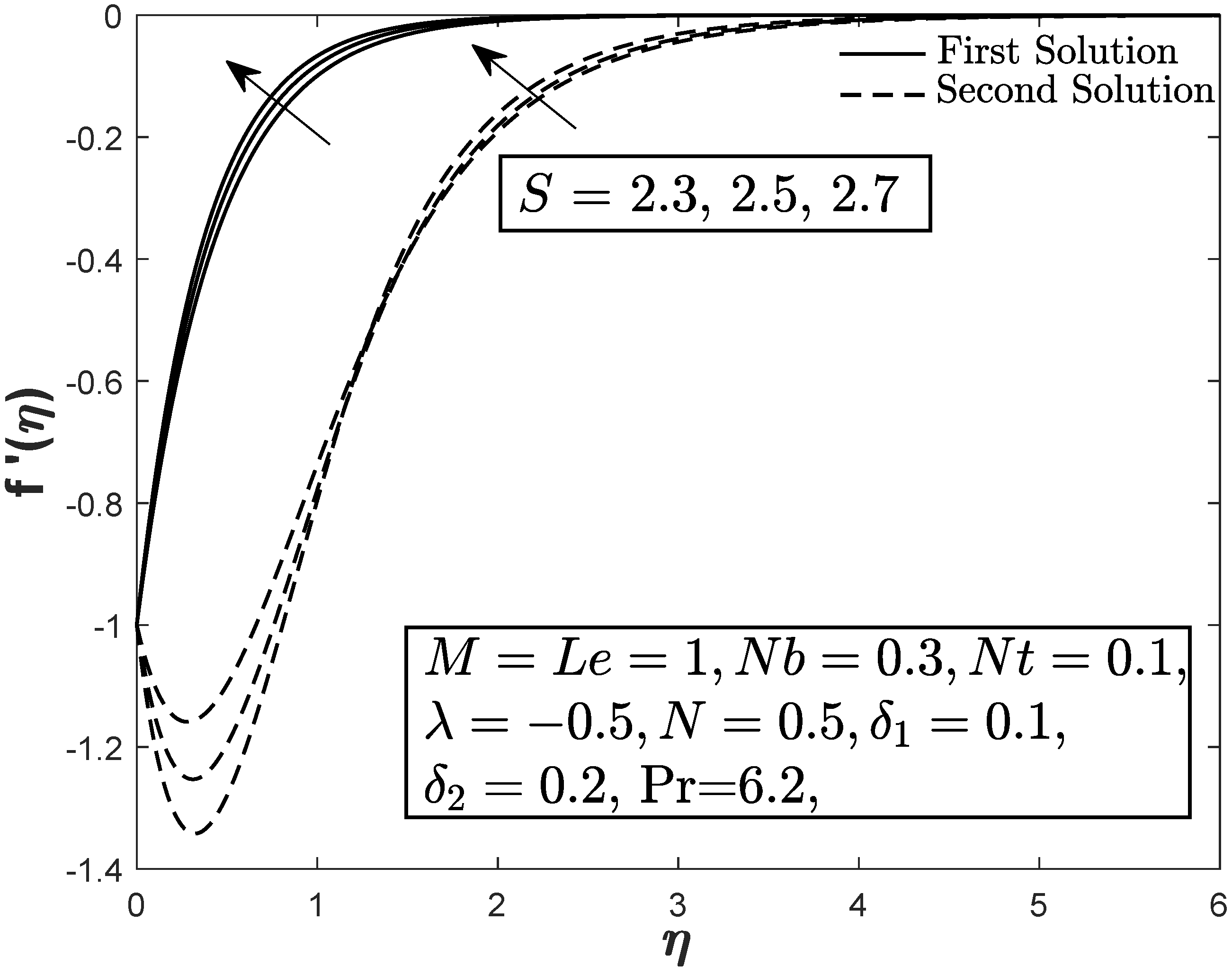
- The skin friction coefficient inflates for the shrinking case , deflates for the stretching case and has no change for the static plate when the suction parameter S is enhanced. Higher values of the suction parameter i.e., also contribute to the appearance of the dual solutions in the present work.
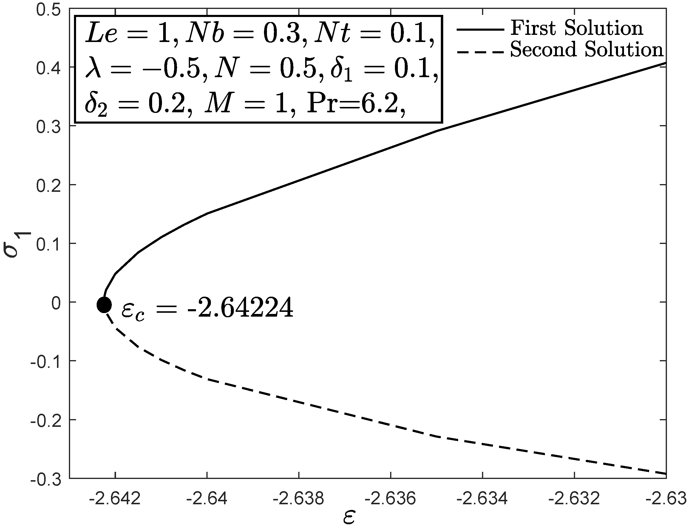
- The stability analysis is conducted and it is mathematically proved that the first solution is the physical/real solution.
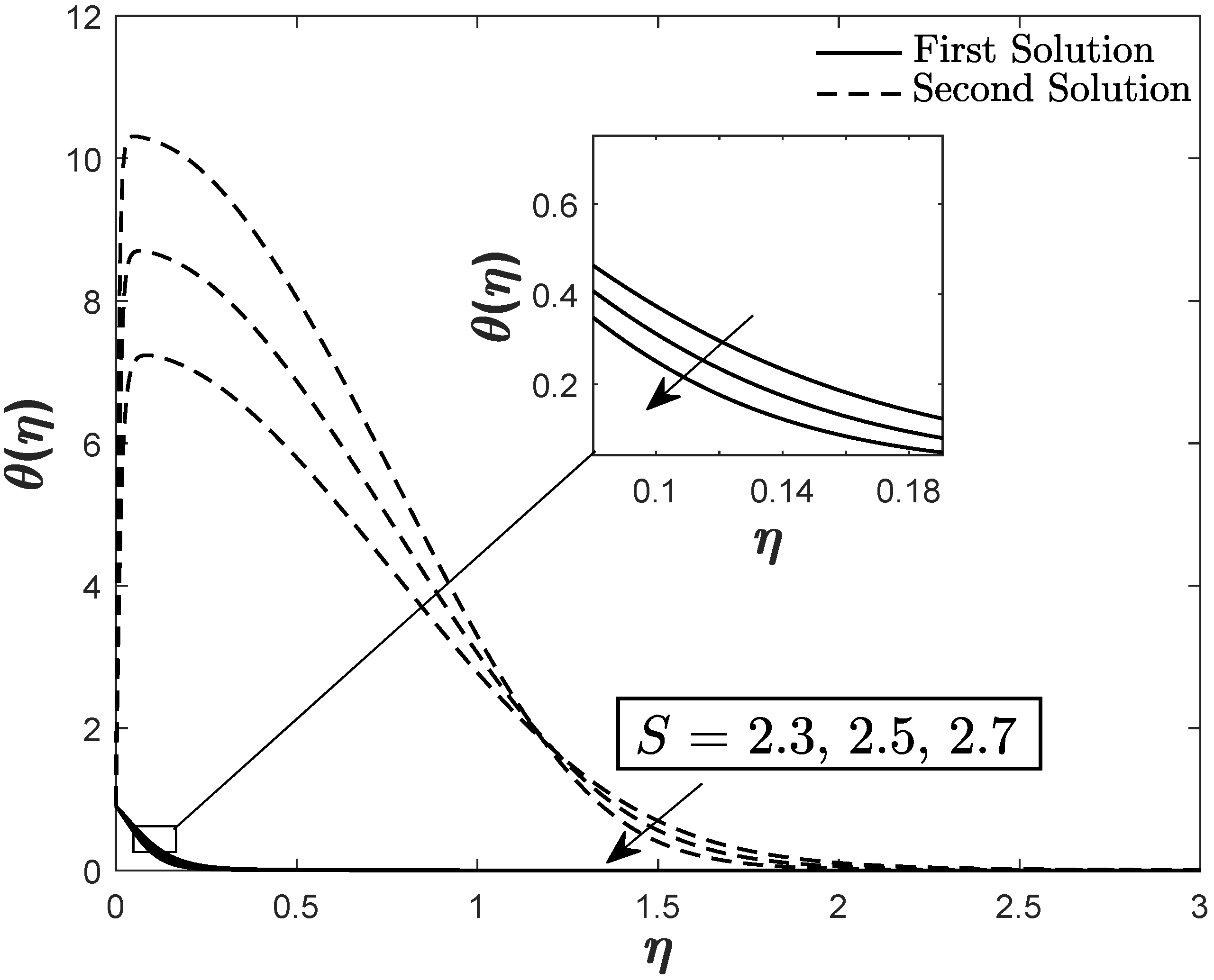
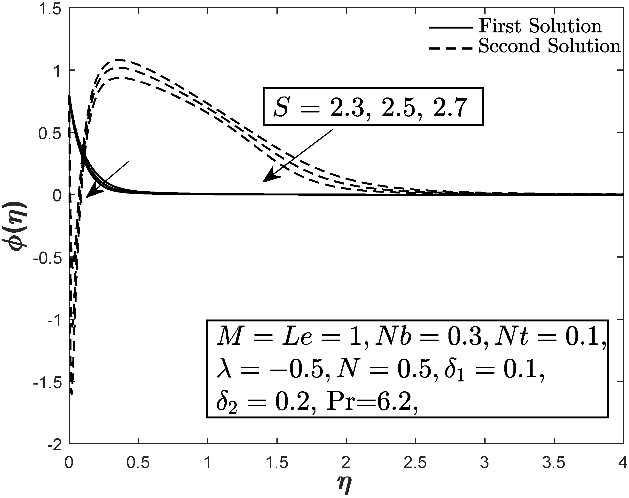
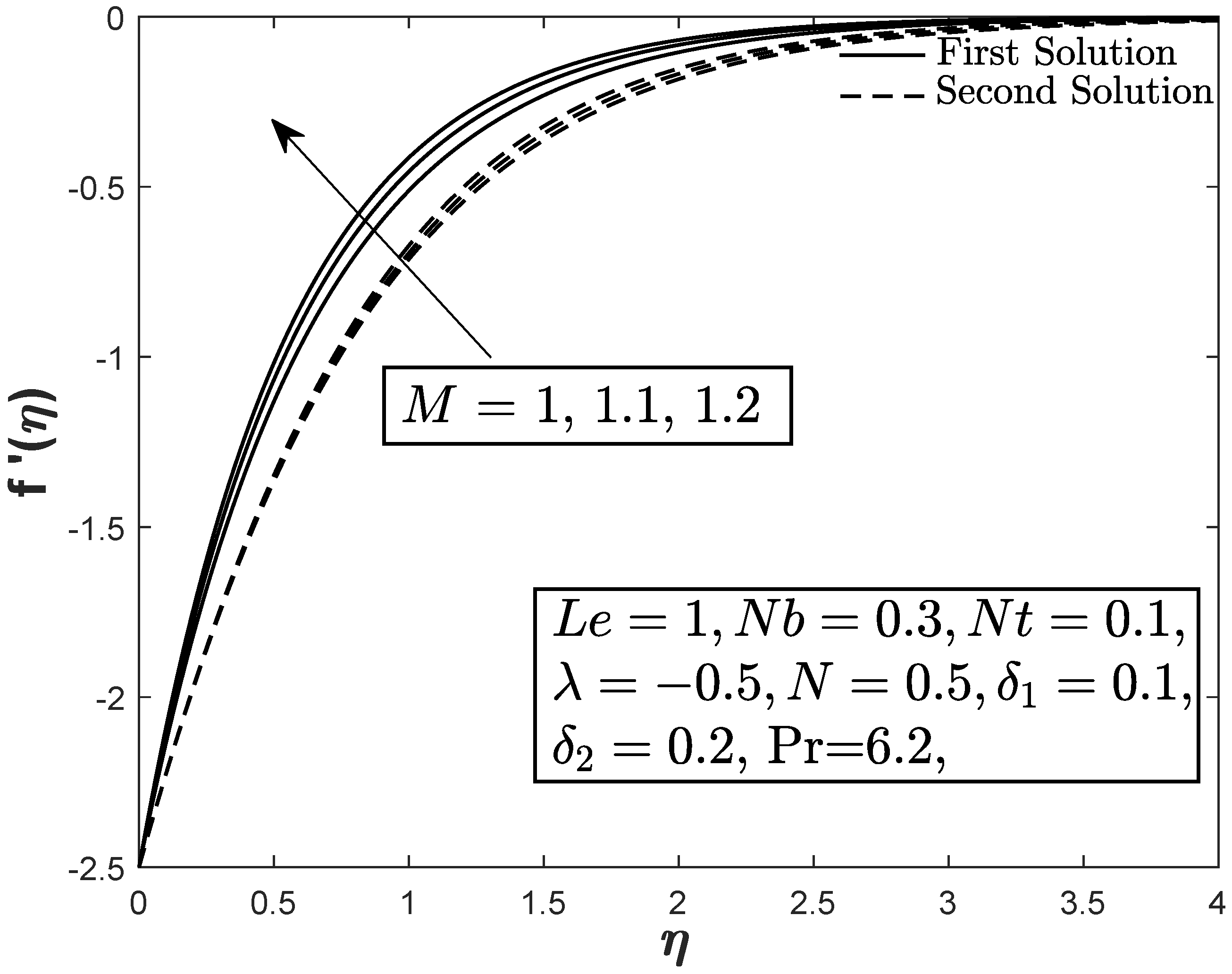
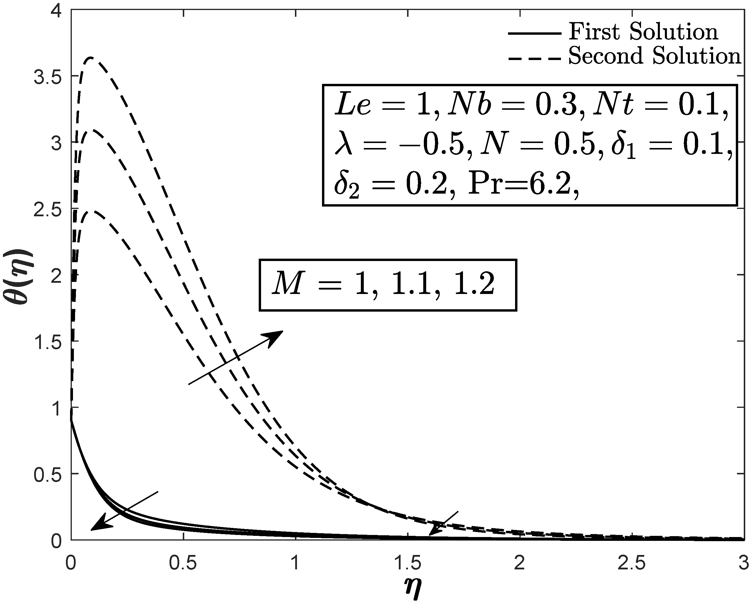
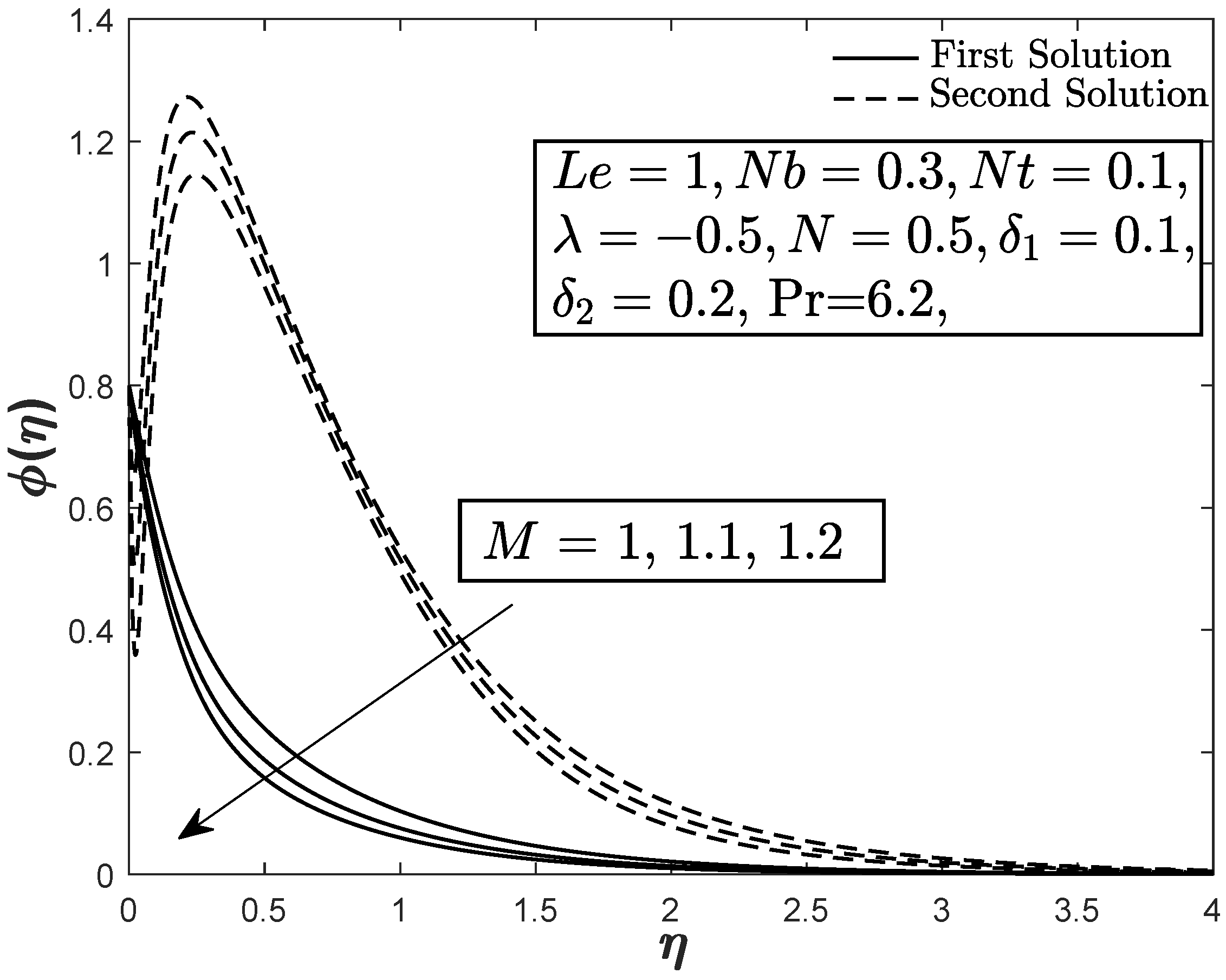
- The combined effects of buoyancy parameter ( and N) with higher values of the suction parameter S in the shrinked flow gave the reverse effect of the Lorentz force to the velocity, temperature and concentration profiles.
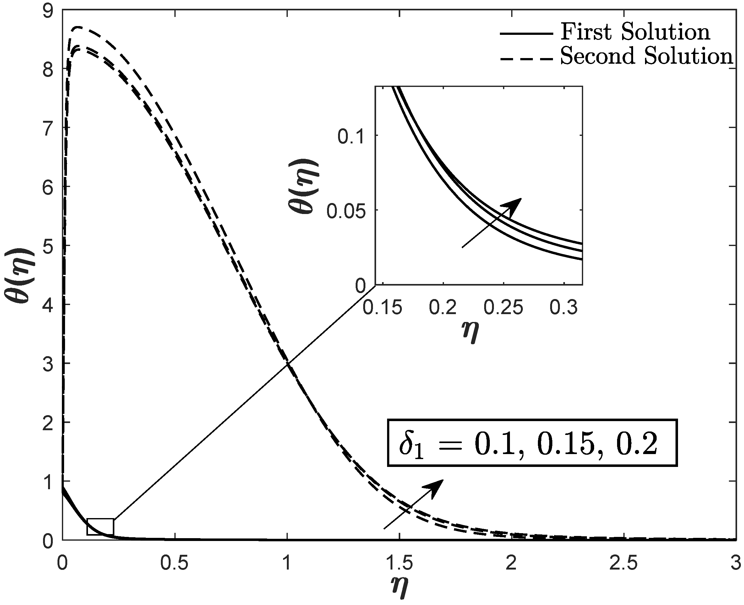
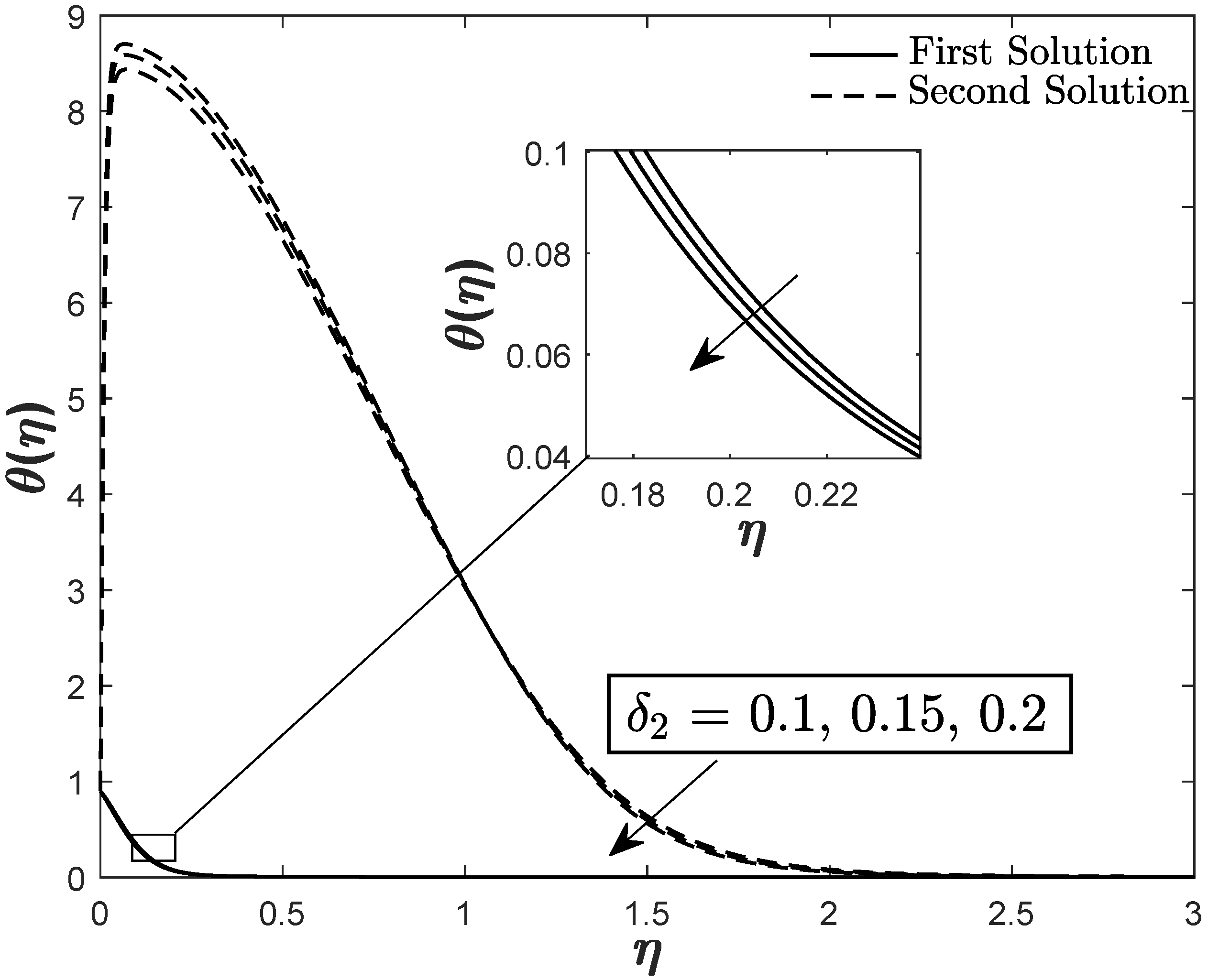
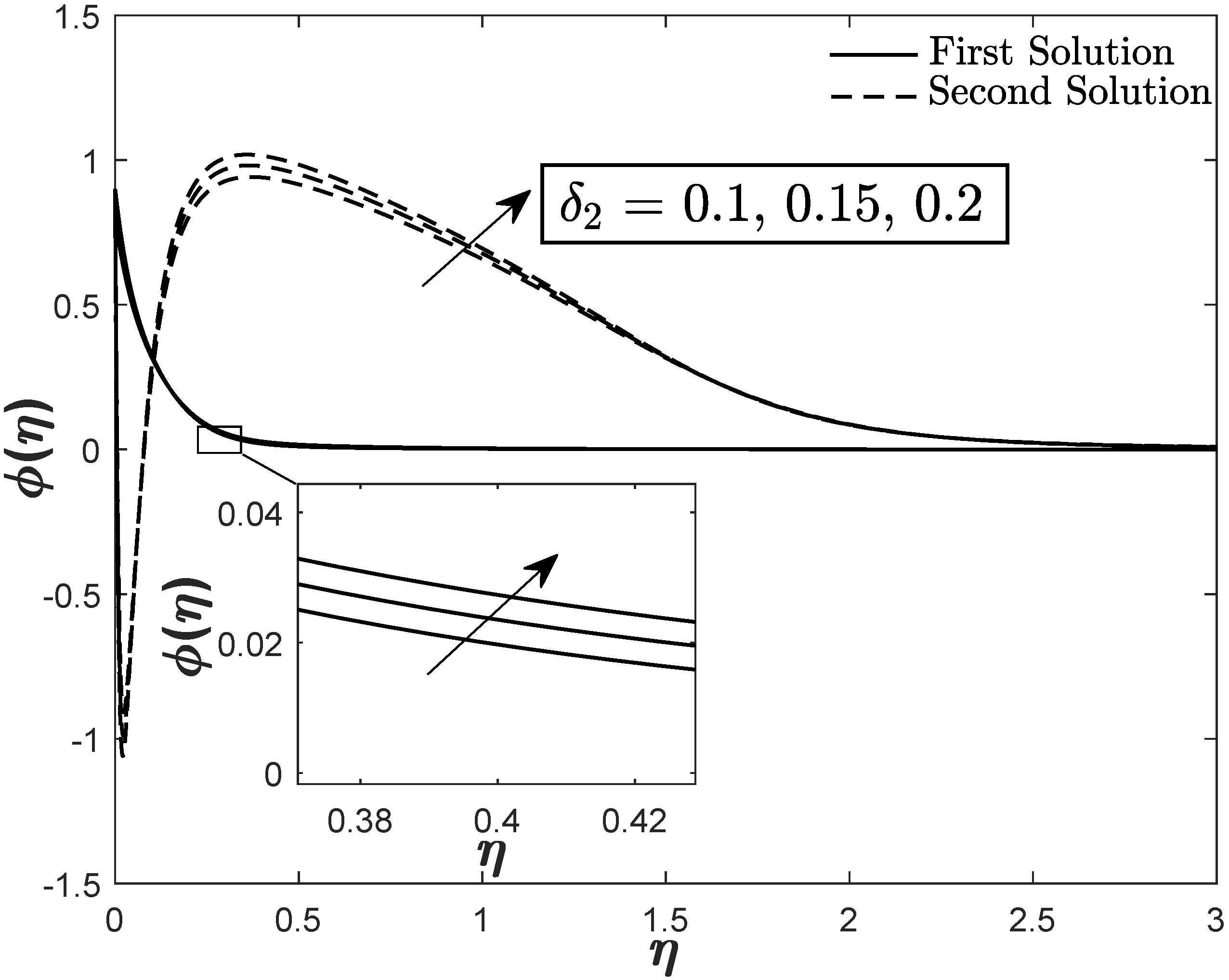
- Both temperature and concentration slightly inclines with the imposition of the thermal and solutal stratification parameters, respectively.
Author Contributions
Acknowledgments
Conflicts of Interest
Abbreviations
| magnitude of the magnetic field strength | |
| C | nanoparticle concentration |
| Brownian diffusion coefficient | |
| thermophoretic diffusion coefficient | |
| Lewis number | |
| M | magnetic parameter |
| N | solutal buoyancy parameter |
| Brownian motion parameter | |
| thermophoresis parameter | |
| Pr | Prandtl number |
| local Reynolds number | |
| T | nanofluid temperature |
| f | dimensionless stream function along direction |
| g | gravitational acceleration |
| t | time |
| velocities in the directions, respectively | |
| coordinate axis align and normal to the sheet | |
| kinematic viscocity | |
| density of base fluid | |
| density of nanoparticles | |
| density of base fluid far from the boundary | |
| thermal expansion coefficient | |
| solutal expansion coefficient | |
| thermal diffusivity of the fluid | |
| dimensionless time variable | |
| ratio of the heat capacity of the nanoparticles to the base fluid | |
| thermal buoyancy parameter | |
| thermal relaxation time | |
| unknown eigenvalue | |
| electrical conductivity of the fluid | |
| dimensionless temperature | |
| dimensionless nanoparticles volume fraction/concentration | |
| thermal relaxation parameter | |
| thermal stratification parameter | |
| solutal stratification parameter |
References
- Crane, L.J. Flow past a stretching plate. Zeitschrift Angewandte Mathematik Physik ZAMP 1970, 21, 645–647. [Google Scholar] [CrossRef]
- Miklavčič, M.; Wang, C. Viscous flow due to a shrinking sheet. Q. Appl. Math. 2006, 64, 283–290. [Google Scholar] [CrossRef]
- Wang, C.Y. Stagnation flow towards a shrinking sheet. Int. J. Non-Linear Mech. 2008, 43, 377–382. [Google Scholar] [CrossRef]
- Fang, T.; Yao, S.; Zhang, J.; Aziz, A. Viscous flow over a shrinking sheet with a second order slip flow model. Commun. Nonlinear Sci. Numer. Simul. 2010, 15, 1831–1842. [Google Scholar] [CrossRef]
- Jusoh, R.; Nazar, R.; Pop, I. Three-dimensional flow of a nanofluid over a permeable stretching/shrinking surface with velocity slip: A revised model. Phys. Fluids 2018, 30, 033604. [Google Scholar] [CrossRef]
- Soomro, F.A.; Zaib, A.; Haq, R.U.; Sheikholeslami, M. Dual nature solution of water functionalized copper nanoparticles along a permeable shrinking cylinder: FDM approach. Int. J. Heat Mass Transf. 2019, 129, 1242–1249. [Google Scholar] [CrossRef]
- Al-Waeli, A.H.; Sopian, K.; Chaichan, M.T.; Kazem, H.A.; Hasan, H.A.; Al-Shamani, A.N. An experimental investigation of SiC nanofluid as a base-fluid for a photovoltaic thermal PV/T system. Energy Conv. Manag. 2017, 142, 547–558. [Google Scholar] [CrossRef]
- Mahian, O.; Kianifar, A.; Kalogirou, S.A.; Pop, I.; Wongwises, S. A review of the applications of nanofluids in solar energy. Int. J. Heat Mass Transf. 2013, 57, 582–594. [Google Scholar] [CrossRef]
- Ebrahimnia-Bajestan, E.; Moghadam, M.C.; Niazmand, H.; Daungthongsuk, W.; Wongwises, S. Experimental and numerical investigation of nanofluids heat transfer characteristics for application in solar heat exchangers. Int. J. Heat Mass Transf. 2016, 92, 1041–1052. [Google Scholar] [CrossRef]
- Kasaeian, A.; Daneshazarian, R.; Mahian, O.; Kolsi, L.; Chamkha, A.J.; Wongwises, S.; Pop, I. Nanofluid flow and heat transfer in porous media: A review of the latest developments. Int. J. Heat Mass Transf. 2017, 107, 778–791. [Google Scholar] [CrossRef]
- Sidik, N.A.; Yazid, M.N.; Mamat, R. A review on the application of nanofluids in vehicle engine cooling system. Int. Commun. Heat Mass Transf. 2015, 68, 85–90. [Google Scholar] [CrossRef]
- Al-Waeli, A.H.; Sopian, K.; Kazem, H.A.; Chaichan, M.T. Photovoltaic Solar Thermal (PV/T) Collectors Past, Present and Future: A Review. Int. J. Appl. Eng. Res. 2016, 11, 10757–10765. [Google Scholar]
- Sarkar, J.; Ghosh, P.; Adil, A. A review on hybrid nanofluids: Recent research, development and applications. Renew. Sust. Energ. Rev. 2015, 43, 164–177. [Google Scholar] [CrossRef]
- Moradikazerouni, A.; Afrand, M.; Alsarraf, J.; Mahian, O.; Wongwises, S.; Tran, M.D. Comparison of the effect of five different entrance channel shapes of a micro-channel heat sink in forced convection with application to cooling a supercomputer circuit board. Appl. Therm. Eng. 2019, 150, 1078–1089. [Google Scholar] [CrossRef]
- Moradikazerouni, A.; Afrand, M.; Alsarraf, J.; Wongwises, S.; Asadi, A.; Nguyen, T.K. Investigation of a computer CPU heat sink under laminar forced convection using a structural stability method. Int. J. Heat Mass Transf. 2019, 134, 1218–1226. [Google Scholar] [CrossRef]
- Buongiorno, J. Convective transport in nanofluids. J. Heat Transf.-Trans. ASME 2006, 128, 240–250. [Google Scholar] [CrossRef]
- Tiwari, R.K.; Das, M.K. Heat transfer augmentation in a two-sided lid-driven differentially heated square cavity utilizing nanofluids. Int. J. Heat Mass Transf. 2007, 50, 2002–2018. [Google Scholar] [CrossRef]
- Khan, W.A.; Pop, I. Boundary-layer flow of a nanofluid past a stretching sheet. Int. J. Heat Mass Transf. 2010, 5, 2477–2483. [Google Scholar] [CrossRef]
- Alsarraf, J.; Moradikazerouni, A.; Shahsavar, A.; Afrand, M.; Salehipour, H.; Tran, M.D. Hydrothermal analysis of turbulent boehmite alumina nanofluid flow with different nanoparticle shapes in a minichannel heat exchanger using two-phase mixture model. Physica A 2019, 520, 275–288. [Google Scholar] [CrossRef]
- Mahmood, A.; Aziz, A.; Jamshed, W.; Hussain, S. Mathematical model for thermal solar collectors by using magnetohydrodynamic Maxwell nanofluid with slip conditions, thermal radiation and variable thermal conductivity. Results Phys. 2017, 7, 3425–3433. [Google Scholar] [CrossRef]
- Aziz, A.; Jamshed, W. Unsteady MHD slip flow of non Newtonian power-law nanofluid over a moving surface with temperature dependent thermal conductivity. Discret. Contin. Dyn. Syst.-Ser. S 2018, 11, 617–630. [Google Scholar] [CrossRef]
- Jamshed, W.; Aziz, A. A comparative entropy based analysis of Cu and Fe3O4/methanol Powell-Eyring nanofluid in solar thermal collectors subjected to thermal radiation, variable thermal conductivity and impact of different nanoparticles shape. Results Phys. 2018, 9, 195–205. [Google Scholar] [CrossRef]
- Aziz, A.; Jamshed, W.; Aziz, T. Mathematical model for thermal and entropy analysis of thermal solar collectors by using Maxwell nanofluids with slip conditions, thermal radiation and variable thermal conductivity. Results Phys. 2018, 16, 123–136. [Google Scholar] [CrossRef]
- Akbar, N.S.; Beg, O.A.; Khan, Z.H. Magneto-nanofluid flow with heat transfer past a stretching surface for the new heat flux model using numerical approach. Int. J. Numer. Methods Heat Fluid Flow 2017, 27, 1215–1230. [Google Scholar] [CrossRef]
- Cattaneo, C. Sulla conduzione del calore. Atti Sem. Mat. Fis. Univ. Modena 1948, 3, 83–101. [Google Scholar]
- Christov, C.I. On frame indifferent formulation of the Maxwell-Cattaneo model of finite-speed heat conduction. Mech. Res. Commun. 2009, 36, 481–486. [Google Scholar] [CrossRef]
- Straughan, B. Thermal convection with the Cattaneo-Christov model. Int. J. Heat Mass Transf. 2010, 53, 95–98. [Google Scholar] [CrossRef]
- Ciarletta, M.; Straughan, B. Uniqueness and structural stability for the Cattaneo-Christov equations. Mech. Res. Commun. 2010, 37, 445–447. [Google Scholar] [CrossRef]
- Tibullo, V.; Zampoli, V. A uniqueness result for the Cattaneo-Christov heat conduction model applied to incompressible fluids. Mech. Res. Commun. 2011, 38, 77–79. [Google Scholar] [CrossRef]
- Mustafa, M. Cattaneo-Christov heat flux model for rotating flow and heat transfer of upper-convected Maxwell fluid. AIP Adv. 2015, 5, 047109. [Google Scholar] [CrossRef]
- Salahuddin, T.; Malik, M.Y.; Hussain, A.; Bilal, S.; Awais, M. MHD flow of Cattanneo-Christov heat flux model for Williamson fluid over a stretching sheet with variable thickness: Using numerical approach. J. Magn. Magn. Mater. 2016, 401, 991–997. [Google Scholar] [CrossRef]
- Hayat, T.; Khan, M.I.; Farooq, M.; Alsaedi, A.; Waqas, M.; Yasmeen, T. Impact of Cattaneo-Christov heat flux model in flow of variable thermal conductivity fluid over a variable thicked surface. Int. J. Heat Mass Transf. 2016, 99, 702–710. [Google Scholar] [CrossRef]
- Malik, M.Y.; Khan, M.; Salahuddin, T.; Khan, I. Variable viscosity and MHD flow in Casson fluid with Cattaneo-Christov heat flux model: Using Keller box method. Eng. Sci. Technol. Int. J. 2016, 19, 1985–1992. [Google Scholar] [CrossRef]
- Kumar, R.K.; Varma, S.V.K. MHD Boundary Layer Flow of Nanofluid Through a Porous Medium Over a Stretching Sheet with Variable Wall Thickness: Using Cattaneo-Christov Heat Flux Model. J. Theor. Appl. Mech. 2018, 48, 72–92. [Google Scholar] [CrossRef]
- Hayat, T.; Khan, M.W.; Alsaedi, A.; Ayub, M.; Khan, M.I. Stretched flow of Oldroyd-B fluid with Cattaneo-Christov heat flux. Results Phys. 2017, 7, 2470–2476. [Google Scholar] [CrossRef]
- Hayat, T.; Khan, M.I.; Waqas, M.; Alsaedi, A. On Cattaneo-Christov heat flux in the flow of variable thermal conductivity Eyring–Powell fluid. Results Phys. 2017, 7, 446–450. [Google Scholar] [CrossRef]
- Hayat, T.; Nadeem, S. Flow of 3D Eyring-Powell fluid by utilizing Cattaneo-Christov heat flux model and chemical processes over an exponentially stretching surface. Results Phys. 2018, 8, 397–403. [Google Scholar] [CrossRef]
- Khan, M. On Cattaneo-Christov heat flux model for Carreau fluid flow over a slendering sheet. Results Phys. 2017, 7, 310–319. [Google Scholar] [CrossRef]
- Li, J.; Zheng, L.; Liu, L. MHD viscoelastic flow and heat transfer over a vertical stretching sheet with Cattaneo-Christov heat flux effects. J. Mol. Liq. 2016, 221, 19–25. [Google Scholar] [CrossRef]
- Nadeem, S.; Ahmad, S.; Muhammad, N. Cattaneo-Christov flux in the flow of a viscoelastic fluid in the presence of Newtonian heating. J. Mol. Liq. 2017, 237, 180–184. [Google Scholar] [CrossRef]
- Khan, M.I.; Zia, Q.Z.; Alsaedi, A.; Hayat, T. Thermally stratified flow of second grade fluid with non-Fourier heat flux and temperature dependent thermal conductivity. Results Phys. 2018, 8, 799–804. [Google Scholar] [CrossRef]
- Hayat, T.; Ahmad, S.; Khan, M.I.; Alsaedi, A. Investigation of generalized Ficks and Fouriers laws in the second-grade fluid flow. Appl. Math. Mech.-Engl. Ed. 2018, 1–4. [Google Scholar] [CrossRef]
- Mahmood, A.; Jamshed, W.; Aziz, A. Entropy and heat transfer analysis using Cattaneo-Christov heat flux model for a boundary layer flow of Casson nanofluid. Results Phys. 2018, 10, 640–649. [Google Scholar] [CrossRef]
- Jamshed, W.; Aziz, A. Cattaneo-Christov based study of TiO2–CuO/EG Casson hybrid nanofluid flow over a stretching surface with entropy generation. Appl. Nanosci. 2018, 8, 685–698. [Google Scholar] [CrossRef]
- Ibrahim, W.; Makinde, O.D. The effect of double stratification on boundary-layer flow and heat transfer of nanofluid over a vertical plate. Comput. Fluids 2013, 86, 433–441. [Google Scholar] [CrossRef]
- Mat Yasin, M.H.; Arifin, N.M.; Nazar, R.; Ismail, F.; Pop, I. Mixed convection boundary layer flow embedded in a thermally stratified porous medium saturated by a nanofluid. Adv. Mech. Eng. 2018, 5, 121943. [Google Scholar] [CrossRef]
- Hussain, T.; Hussain, S.; Hayat, T. Impact of double stratification and magnetic field in mixed convective radiative flow of Maxwell nanofluid. J. Mol. Liq. 2016, 220, 870–878. [Google Scholar] [CrossRef]
- Abbasi, F.M.; Shehzad, S.A.; Hayat, T.; Alhuthali, M.S. Mixed convection flow of jeffrey nanofluid with thermal radiation and double stratification. J. Hydrodyn. 2016, 28, 840–849. [Google Scholar] [CrossRef]
- Besthapu, P.; Haq, R.U.; Bandari, S.; Al-Mdallal, Q.M. Mixed convection flow of thermally stratified MHD nanofluid over an exponentially stretching surface with viscous dissipation effect. J. Taiwan Inst. Chem. Eng. 2017, 71, 307–314. [Google Scholar] [CrossRef]
- Daniel, Y.S.; Aziz, Z.A.; Ismail, Z.; Salah, F. Effects of thermal radiation, viscous and Joule heating on electrical MHD nanofluid with double stratification. Chin. J. Phys. 2017, 55, 630–651. [Google Scholar] [CrossRef]
- Daniel, Y.S.; Aziz, Z.A.; Ismail, Z.; Salah, F. Double stratification effects on unsteady electrical MHD mixed convection flow of nanofluid with viscous dissipation and Joule heating. J. Appl. Res. Technol. 2017, 15, 464–476. [Google Scholar] [CrossRef]
- Kandasamy, R.; Dharmalingam, R.; Prabhu, K.S. Thermal and solutal stratification on MHD nanofluid flow over a porous vertical plate. Alexandria Eng. J. 2018, 57, 121–130. [Google Scholar] [CrossRef]
- Hayat, T.; Naz, S.; Waqas, M.; Alsaedi, A. Effectiveness of Darcy-Forchheimer and nonlinear mixed convection aspects in stratified Maxwell nanomaterial flow induced by convectively heated surface. Appl. Math. Mech.-Engl. Ed. 2018, 39, 1373–1384. [Google Scholar] [CrossRef]
- Anwar, M.I.; Khan, I.; Sharidan, S.; Salleh, M.Z. Conjugate effects of heat and mass transfer of nanofluids over a nonlinear stretching sheet. Int. J. Phys. Sci. 2012, 7, 4081–4092. [Google Scholar] [CrossRef]
- Ismail, N.S.; Arifin, N.M.; Nazar, R.; Bachok, N. Stability analysis of unsteady MHD stagnation point flow and heat transfer over a shrinking sheet in the presence of viscous dissipation. Chin. J. Phys. 2019, 57, 116–126. [Google Scholar] [CrossRef]
- Ismail, N.S.; Arifin, N.M.; Nazar, R. The stagnation-point flow and heat transfer of nanofluid over a shrinking surface in magnetic field and thermal radiation with slip effects: A stability analysis. J. Phys. Conf. Ser. 2017, 890, 012055. [Google Scholar] [CrossRef]
- Ismail, N.S.; Arifin, N.M.; Nazar, R.; Bachok, N.; Mahiddin, N. Stability analysis in stagnation-point flow towards a shrinking sheet with homogeneous–Heterogeneous reactions and suction effects. Int. J. Appl. Eng. Res. 2016, 11, 9229–9235. [Google Scholar]
- Bakar, S.A.; Arifin, N.M.; Md Ali, F.; Bachok, N.; Nazar, R.; Pop, I. A stability analysis on mixed convection boundary layer flow along a permeable vertical cylinder in a porous medium filled with a nanofluid and thermal radiation. Appl. Sci. 2018, 8, 483. [Google Scholar] [CrossRef]
- Bakar, S.A.; Arifin, N.M.; Nazar, R.; Ali, F.M.; Bachok, N.; Pop, I. The effects of suction on forced convection boundary layer stagnation point slip flow in a darcy porous medium towards a shrinking sheet with presence of thermal radiation: A stability analysis. J. Porous Media 2018, 21. [Google Scholar] [CrossRef]
- Anuar, N.; Bachok, N.; Pop, I. A stability analysis of solutions in boundary layer flow and heat transfer of carbon nanotubes over a moving plate with slip effect. Energies 2018, 11, 3243. [Google Scholar] [CrossRef]
- Salleh, S.N.A.; Bachok, N.; Arifin, N.M.; Ali, F.M.; Pop, I. Stability analysis of mixed convection flow towards a moving thin needle in nanofluid. Appl. Sci. 2018, 8, 842. [Google Scholar] [CrossRef]
- Salleh, S.; Bachok, N.; Arifin, N.M.; Ali, F.; Pop, I. Magnetohydrodynamics flow past a moving vertical thin needle in a nanofluid with stability analysis. Energies 2018, 11, 3297. [Google Scholar] [CrossRef]
- Najib, N.; Bachok, N.; Arifin, N.M.; Ali, F.M. Stability analysis of stagnation-point flow in a nanofluid over a stretching/shrinking sheet with second-order slip, soret and dufour effects: A revised model. Appl. Sci. 2018, 8, 642. [Google Scholar] [CrossRef]
- Jamaludin, A.; Nazar, R.; Pop, I. Three-dimensional magnetohydrodynamic mixed convection flow of nanofluids over a nonlinearly permeable stretching/shrinking sheet with velocity and thermal slip. Appl. Sci. 2018, 8, 1128. [Google Scholar] [CrossRef]
- Yahaya, R.; Md Arifin, N.; Mohamed Isa, S. Stability analysis on magnetohydrodynamic flow of casson fluid over a shrinking sheet with homogeneous-heterogeneous reactions. Entropy 2018, 20, 652. [Google Scholar] [CrossRef]
- Jamaludin, A.; Nazar, R.; Pop, I. Three-dimensional mixed convection stagnation-point flow over a permeable vertical stretching/shrinking surface with a velocity slip. Chin. J. Phys. 2017, 55, 1865–1882. [Google Scholar] [CrossRef]
- Rahman, M.M. Effects of second-order slip and magnetic field on mixed convection stagnation-point flow of a Maxwellian fluid: Multiple solutions. J. Heat Transf.-Trans. ASME 2016, 138, 122503. [Google Scholar] [CrossRef]
- Borrelli, A.; Giantesio, G.; Patria, M.C.; Roşca, N.C.; Roşca, A.V.; Pop, I. Buoyancy effects on the 3D MHD stagnation-point flow of a Newtonian fluid. Commun. Nonlinear Sci. Numer. Simul. 2017, 43, 1–3. [Google Scholar] [CrossRef]
- Rashidi, M.M.; Rostami, B.; Freidoonimehr, N.; Abbasbandy, S. Free convective heat and mass transfer for MHD fluid flow over a permeable vertical stretching sheet in the presence of the radiation and buoyancy effects. Ain Shams Eng. J. 2014, 5, 901–912. [Google Scholar] [CrossRef]


| Pr | Present | Khan and Pop [18] | Akbar et al. [24] | ||
|---|---|---|---|---|---|
| 0.07 | 0.066056 | 0.0663 | 0.3694% | 0.0663 | 0.3694% |
| 0.2 | 0.169089 | 0.1691 | 0.0065% | 0.1691 | 0.0065% |
| 0.7 | 0.453916 | 0.4539 | 0.0035% | 0.4539 | 0.0035% |
| 2 | 0.911358 | 0.9113 | 0.0064% | 0.9114 | 0.0046% |
| 7 | 1.895403 | 1.8954 | 0.0001% | 1.8954 | 0.0001% |
| 20 | 3.353904 | 3.3539 | 0.0001% | 3.3539 | 0.0001% |
| 70 | 6.462199 | 6.4621 | 0.0015% | 6.4622 | 0.0000% |
| Present | Abbasi et al. [48] | |||||
|---|---|---|---|---|---|---|
| 0 | 0.82851 | 0.37980 | 0.82852 | 0.37977 | 0.0012% | 0.0079% |
| 0.05 | 0.85574 | 0.35713 | - | - | - | - |
| 0.1 | 0.88282 | 0.33457 | - | - | - | - |
| Shrinking | Stretching | |||
|---|---|---|---|---|
| 0 | 4.466687 | 8.429299 | 5.055202 | 10.790924 |
| 0.005 | 4.743514 (+5.83%) | 8.335221 (−1.13%) | 5.395635 (+6.31%) | 10.682332 (−1.02%) |
| 0.01 | 5.052113 (+11.59%) | 8.230340 (−2.42%) | 5.752854 (+12.13%) | 10.568364 (−2.10%) |
© 2019 by the authors. Licensee MDPI, Basel, Switzerland. This article is an open access article distributed under the terms and conditions of the Creative Commons Attribution (CC BY) license (http://creativecommons.org/licenses/by/4.0/).
Share and Cite
Safwa Khashi’ie, N.; Md Arifin, N.; Hafidzuddin, E.H.; Wahi, N. Dual Stratified Nanofluid Flow Past a Permeable Shrinking/Stretching Sheet Using a Non-Fourier Energy Model. Appl. Sci. 2019, 9, 2124. https://doi.org/10.3390/app9102124
Safwa Khashi’ie N, Md Arifin N, Hafidzuddin EH, Wahi N. Dual Stratified Nanofluid Flow Past a Permeable Shrinking/Stretching Sheet Using a Non-Fourier Energy Model. Applied Sciences. 2019; 9(10):2124. https://doi.org/10.3390/app9102124
Chicago/Turabian StyleSafwa Khashi’ie, Najiyah, Norihan Md Arifin, Ezad Hafidz Hafidzuddin, and Nadihah Wahi. 2019. "Dual Stratified Nanofluid Flow Past a Permeable Shrinking/Stretching Sheet Using a Non-Fourier Energy Model" Applied Sciences 9, no. 10: 2124. https://doi.org/10.3390/app9102124
APA StyleSafwa Khashi’ie, N., Md Arifin, N., Hafidzuddin, E. H., & Wahi, N. (2019). Dual Stratified Nanofluid Flow Past a Permeable Shrinking/Stretching Sheet Using a Non-Fourier Energy Model. Applied Sciences, 9(10), 2124. https://doi.org/10.3390/app9102124