Simulation-Supported Testing of Smart Energy Product Prototypes


Abstract
1. Introduction
2. Materials and Methods
2.1. Simulation Environment Testing
- Energy generation was modelled using a DC voltage/current source, which simulated a residential PV system. Energy consumption, on the other hand, was modelled using an RLC controllable load, which consumed the generated power or drew power from the local grid whenever consumption exceeded generation.
- The laboratory’s main measurement system integrated these two inputs and periodically passed them on to the HEMP prototype using the communication infrastructure, which consisted of a custom-built middleware application linking these components.
- The prototype calculated the key indicator’s new value and set the corresponding LED properties.
2.2. Scenario-Based Simulations
- Summer Load Profile, Inadequate PV Production
- Summer Load Profile, Adequate PV Production
- Winter Load Profile, Inadequate PV Production
- Winter Load Profile, Adequate PV Production
2.3. End User Testing
3. Results
3.1. Simulation Environment Test Results
3.1.1. Bodhi
3.1.2. CrystalLight
3.1.3. LightInsight
3.2. Scenario Simulation Results
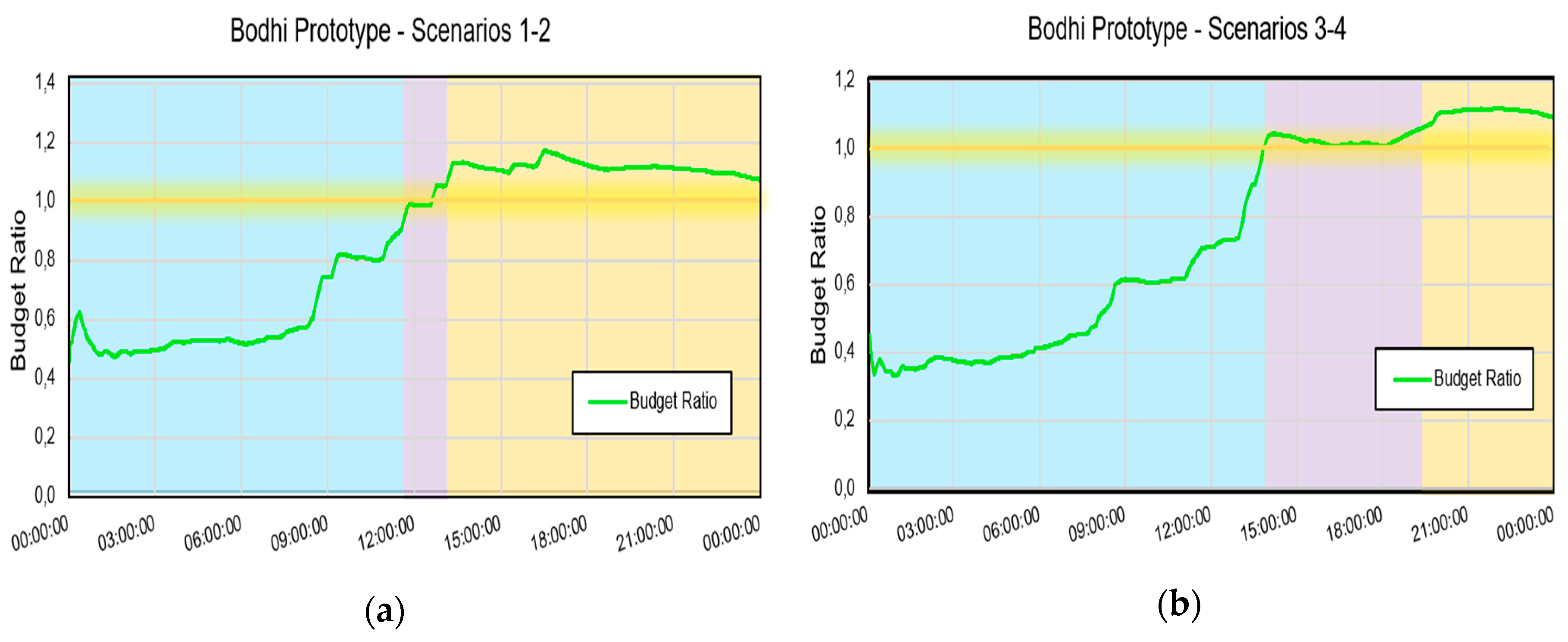
3.2.1. Bodhi
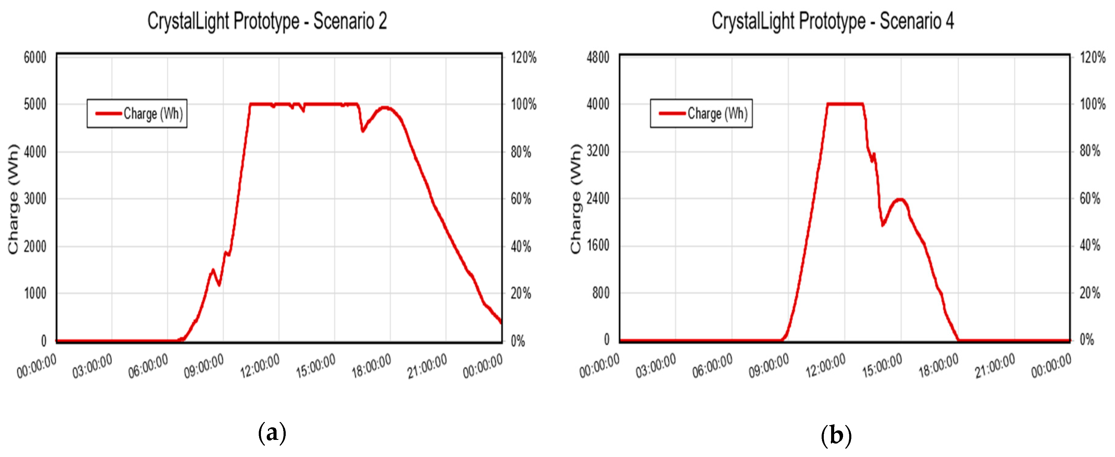
3.2.2. CrystalLight
3.2.3. LightInsight
3.3. End User Testing Results
3.3.1. Bodhi
3.3.2. LightInsight
4. Discussion and Conclusions
Author Contributions
Funding
Acknowledgments
Conflicts of Interest
References
- Reinders, A.; De Respinis, M.; Van Loon, J.; Stekelenburg, A.; Bliek, F.; Schram, W.; van Sark, W.; Esteri, T.; Übermasser, S.; Lehfuss, F.; et al. Co-evolution of smart energy products and services: A novel approach towards smart grids. In Proceedings of the Asian Conference on Energy, Power and Transportation Electrification, ACEPT 2016, Singapore, 25–27 October.
- Lannoye, E.; Flynn, D.; O’Malley, M. Evaluation of Power System Flexibility. IEEE Trans. Power Syst. 2012, 27, 922–931. [Google Scholar] [CrossRef]
- Smale, R.; van Vliet, B.; Spaargaren, G. When social practices meet smart grids: Flexibility, grid management, and domestic consumption in The Netherlands. Energy Res. Soc. Sci. 2017, 34, 132–140. [Google Scholar] [CrossRef]
- Gercek, C.; Reinders, A. Smart Appliances for Efficient Integration of Solar Energy: A Dutch Case Study of a Residential Smart Grid Pilot. Appl. Sci. 2019, 9, 581. [Google Scholar] [CrossRef]
- Zhang, Z.; Gercek, C.; Renner, H.; Reinders, A.; Fickert, L. Resonance Instability of Photovoltaic E-Bike Charging Stations: Control Parameters Analysis, Modeling and Experiment. Appl. Sci. 2019, 9, 252. [Google Scholar] [CrossRef]
- Reinders, A.; Übermasser, S.; Van Sark, W.; Gercek, C.; Schram, W.; Obinna, U.; Lehfuss, F.; Van Mierlo, B.; Robledo, C.; Van Wijk, A. An Exploration of the Three-Layer Model Including Stakeholders, Markets and Technologies for Assessments of Residential Smart Grids. Appl. Sci. 2018, 8, 2363. [Google Scholar] [CrossRef]
- Robledo, C.B.; Oldenbroek, V.; Abbruzzese, F.; van Wijk, A.J.M. Integrating a hydrogen fuel cell electric vehicle with vehicle-to-grid technology, photovoltaic power and a residential building. Appl. Energy 2018, 215, 615–629. [Google Scholar] [CrossRef]
- Mwasilu, F.; Justo, J.J.; Kim, E.; Do, T.D.; Jung, J. Electric vehicles and smart grid interaction: A review on vehicle to grid and renewable energy sources integration. Renew. Sustain. Energy Rev. 2014, 34, 501–516. [Google Scholar] [CrossRef]
- Schram, W.L.; Lampropoulos, I.; van Sark, W.G.J.H.M. Photovoltaic systems coupled with batteries that are optimally sized for household self-consumption: Assessment of peak shaving potential. Appl. Energy 2018, 223, 69–81. [Google Scholar] [CrossRef]
- Posma, J.; Lampropoulos, I.; Schram, W.; van Sark, W. Provision of Ancillary Services from an Aggregated Portfolio of Residential Heat Pumps on the Dutch Frequency Containment Reserve Market. Appl. Sci. 2019, 9, 590. [Google Scholar] [CrossRef]
- Van Dam, S.; Bakker, C.; van Hal, J. Home energy monitors: Impact over the medium-term. Build. Res. Inf. 2010, 38, 458–469. [Google Scholar] [CrossRef]
- Geelen, D.; Reinders, A.; Keyson, D. Empowering the end-user in smart grids: Recommendations for the design of products and services. Energy Policy 2013, 61, 151–161. [Google Scholar] [CrossRef]
- Hargreaves, T.; Nye, M.; Burgess, J. Making energy visible: A qualitative field study of how householders interact with feedback from smart energy monitors. Energy Policy 2010, 38, 6111–6119. [Google Scholar] [CrossRef]
- Van Mierlo, B. Users Empowered in Smart Grid Development? Assumptions and Up-To-Date Knowledge. Appl. Sci. 2019, 9, 815. [Google Scholar] [CrossRef]
- Obinna, U.; Joore, P.; Wauben, L.; Reinders, A. Insights from Stakeholders of Five Residential Smart Grid Pilot Projects in the Netherlands. Smart Grid Renew. Energy 2016, 7, 1–15. [Google Scholar] [CrossRef]
- Wolsink, M. The research agenda on social acceptance of distributed generation in smart grids: Renewable as common pool resources. Renew. Sustain. Energy Rev. 2012, 16, 822–835. [Google Scholar] [CrossRef]
- Palensky, P.; van der Meer, A.A.; Lopez, C.D.; Joseph, A.; Pan, K. Cosimulation of intelligent power systems. IEEE Ind. Electron. Mag. 2017, 11, 34–50. [Google Scholar] [CrossRef]
- Godfrey, T.; Mullen, S.; Dugan, R.C.; Rodine, C.; Griffith, D.W.; Golmie, N. Modeling Smart Grid Applications with Co-Simulation. In Proceedings of the 2010 First IEEE International Conference on Smart Grid Communications, Gaithersburg, MD, USA, 4–6 October 2010. [Google Scholar]
- Faruque, M.O.; Sloderbeck, M.; Steurer, M.; Dinavahi, V. Thermoelectric co-simulation on geographically distributed real-time simulators. In Proceedings of the IEEE PES General Meeting, Calgary, AB, Canada, 26–30 July 2009; pp. 1–7. [Google Scholar]
- Georg, H.; Muller, S.; Rehtanz, C.; Wietfeld, C. Analyzing cyber-physical energy systems: The INSPIRE cosimulation of power and ICT systems using HLA. IEEE Trans. Ind. Inf. 2013, 10, 2364–2373. [Google Scholar] [CrossRef]
- Khan, M.; Silva, B.N.; Han, K. Internet of Things Based Energy Aware Smart Home Control System. IEEE Access. 2016, 4, 7556–7566. [Google Scholar] [CrossRef]
- Guenther, C.; Schott, B.; Hennings, W.; Waldowski, P.; Danzer, M.A. Model-based investigation of electric vehicle battery aging by means of vehicle-to-grid scenario simulations. J. Power Sour. 2013, 239, 604–610. [Google Scholar] [CrossRef]
- Vardakas, J.S.; Zorba, N.; Verikoukis, C.V. Performance evaluation of power demand scheduling scenarios in a smart grid environment. Appl. Energy 2015, 142, 164–178. [Google Scholar] [CrossRef]
- Liedtke, C.; Baedeker, C.; Hasselkuss, M.; Rohn, H.; Grinewitschus, V. User-integrated innovation in Sustainable LivingLabs: An experimental infrastructure for researching and developing sustainable product service systems. J. Clean. Prod. 2015, 97, 106–116. [Google Scholar] [CrossRef]
- Ceschin, F. Critical factors for implementing and diffusing sustainable product-Service systems: Insights from innovation studies and companies’ experiences. J. Clean. Prod. 2013, 45, 74–88. [Google Scholar] [CrossRef]
- AIT SmartEST Laboratory for Smart Grids (Fact Sheet). Available online: https://www.ait.ac.at/fileadmin/mc/energy/downloads/Smart_Grids/Produktblatt_CI_SmartEST_lowRes.pdf (accessed on 2 April 2019).
- Chavali, P.; Yang, P.; Nehorai, A. A Distributed Algorithm of Appliance Scheduling for Home Energy Management System. IEEE Trans. Smart Grid 2014, 5, 282–290. [Google Scholar] [CrossRef]


© 2019 by the authors. Licensee MDPI, Basel, Switzerland. This article is an open access article distributed under the terms and conditions of the Creative Commons Attribution (CC BY) license (http://creativecommons.org/licenses/by/4.0/).
Share and Cite
Sierra, A.; Gercek, C.; Übermasser, S.; Reinders, A. Simulation-Supported Testing of Smart Energy Product Prototypes. Appl. Sci. 2019, 9, 2030. https://doi.org/10.3390/app9102030
Sierra A, Gercek C, Übermasser S, Reinders A. Simulation-Supported Testing of Smart Energy Product Prototypes. Applied Sciences. 2019; 9(10):2030. https://doi.org/10.3390/app9102030
Chicago/Turabian StyleSierra, Alonzo, Cihan Gercek, Stefan Übermasser, and Angèle Reinders. 2019. "Simulation-Supported Testing of Smart Energy Product Prototypes" Applied Sciences 9, no. 10: 2030. https://doi.org/10.3390/app9102030
APA StyleSierra, A., Gercek, C., Übermasser, S., & Reinders, A. (2019). Simulation-Supported Testing of Smart Energy Product Prototypes. Applied Sciences, 9(10), 2030. https://doi.org/10.3390/app9102030