1. Introduction
The investigation of natural organic matter (NOM) and especially its dissolved fraction (DOM) is of high relevance in aquatic sciences. Studies of NOM and DOM include their sinks and sources as part of the global carbon cycle [
1,
2,
3,
4], its stability and degradability by abiotic and biotic processes [
5,
6], as well as natural and anthropogenic ecosystem effects e.g., from hydrocarbons [
7]. Complementary to laboratory approaches, the need to measure DOM directly in the water column (in situ) initiated the development of field-applicable optical sensors that can be attached to autonomous vehicles or ship-based platforms [
8]. Addressing the optical properties, namely absorption and fluorescence, of certain DOM fractions in situ sensors enable a high-resolution assessment of these ecosystem-relevant parameters or proxies on different observation platforms [
9,
10]. The absorption of light from fractions of the DOM pool is a long known feature, which was initially investigated by the German chemist Kurt Kalle in the early 20th century [
11]. Observing an increased absorption of light towards the blue and ultraviolet (UV) part of the spectrum, he denoted this fraction of DOM as ‘Gelbstoff’ or ‘yellow substance’ [
12,
13], apparently inspired by the yellowish color of the samples taken from the Baltic Sea. Nowadays, this fraction is known as colored or chromophoric dissolved organic matter, short CDOM [
14,
15]. The measurement principle for CDOM absorption (an inherent optical property, or IOP, of natural water bodies) is based on the reduction of light intensity from a light source to a detector over a certain distance. It typically requires a filtered water sample, since only the dissolved and not the particulate fraction is of interest, and the latter could introduce errors due to light scattering. While in situ filtration is technically possible and practiced e.g., in underway systems [
16], it is rather sophisticated and therefore not realized in today’s commercially submersible CDOM sensors [
17]. For a feasible, but still technically complex, approach to derive CDOM absorption in subsea or underway applications, the scattering loss of photons is suppressed by reflective tubes [
18] or a reflecting cavity [
19,
20,
21]. Yet in the majority of today’s observing platforms and ship operated sensor systems, CDOM absorption measurements are not implemented.
The most common sensors within CTD-samplers, FerryBox systems, autonomous underwater vehicles (AUVs), gliders, biogeochemical Argo floats and alike are CDOM fluorometers. Applying a UV light source and detecting an emitted fluorescence signal at a higher wavelength (lower energy), these sensors utilize a principle that Kalle once described as ‘skyblue fluorescence’ [
12,
22]. In addition to these single-channel sensors, a few sensor systems commercially exist that enable a selection of several wavelengths pairs [
17]. Recently, a matrix fluorescence sensor was presented that can sense a set of 4 detection wavelengths for three different excitation wavelengths, thus spanning a matrix of 12 combinations [
23]. While CDOM fluorescence is technically speaking a correct term, it can be mixed up with CDOM (by definition an absorption property) and reports or commercial product descriptions sometimes tend to incorrectly shorten measurement devices as ‘CDOM sensors’. To reflect the fact that the fluorescing part of the DOM is a subfraction of the absorbing fraction of DOM, we herein use FDOM as a designator for fluorescent DOM, as common in recent literature [
9,
24,
25,
26]. Laboratory measurement of FDOM is typically performed with UV–VIS spectrofluorometers [
27,
28]. They enable a free selection of excitation and detection wavelengths and thus different forms of results: (a) emission spectra (with a fixed excitation wavelength); (b) excitation spectra (with a fixed emission wavelength); (c) synchronous scans (excitation and emission changing at the same rate); and (d) excitation–emission matrices (EEM). The latter provides a full scan of a range of excitation wavelengths, performing for each of these excitation wavelengths a full emission scan. The resulting matrix of fluorescence intensities, sometimes referred to as ‘optical fingerprint’, is reflecting all fluorescing components and its peaks are associated with different components from the DOM pool [
14,
29]. A classical labeling of the fluorophores in DOM identifies five main peaks A, C, B, T, and M. Those peaks are extensively used to identify the main composition and origin of FDOM. Previous reports indicate the correlation between microbial presence and freshly produced DOM (peaks M, B and T), while allochthonous DOM has been associated to the peaks A and C [
29]. EEM spectra are frequently used in recent literature [
27,
28] and several parameters are calculated from them, including the humification index [
30], biological index [
31], and recently produced material index [
32]. A statistical analysis of EEM spectra is often performed by parallel factor analysis (PARAFAC), a method that identifies the underlying components from a set of spectra [
33,
34]. EEM spectroscopy (EEMS) and its spectral analysis can be considered the state-of-the-art in FDOM assessment, however, to the best of our knowledge, no submersible sensor exists that enables the high-resolution (in terms of wavelengths intervals) measurement of excitation–emission matrix spectra with in situ equipment.
Herein, we will present (i) design and application of a novel in situ EEMS sensor system (in memory of Kurt Kalle named the ‘Kallemeter’) that enables full optical fingerprints in a submersible design, and compare these results with (ii) flow-through data from two commercial FDOM sensors, and (iii) spectral components identified in surface water samples from a laboratory UV–VIS spectrofluorometer, based on a field campaign in the Trondheimsfjord, Norway.
2. Materials and Methods
The following section starts with a detailed description of the design of the novel ‘Kallemeter’ in situ EEMS sensor system, including initial laboratory measurements to illustrate its performance. To enable a comparison of bulk fluorescence detected, two commercial FDOM sensors will briefly be introduced, both operated in a commercially available flow-through sensor system (FerryBox, -4H-JENA engineering, Jena, Germany). This will be followed by a description of the laboratory methods applied on discrete water samples, and the subsequently used statistical method to derive the components of the EEM spectra observed. Finally, we will provide information about the study site itself.
2.1. Design of an In Situ Capable EEMS Sensor System
The newly-developed submersible EEMS sensor system provides comprehensive excitation–emission matrices for in situ fluorescence measurements of organic matter in natural waters. This subchapter presents its design, beginning with a representation of the operation mode in
Section 2.1.1. Followed by this, a description of the technical implementation and the system design is given in
Section 2.1.2.
Section 2.1.3 presents the evaluation of the system performance.
2.1.1. Submersible EEMS Sensor System and Modes of Operation
Investigations on fluorescent organic matter can benefit from spatiotemporal information that enable a comprehensive interpretation of the dataset in context of environmental conditions. The ‘Kallemeter’ EEMS sensor system supports in situ explorations with three common modes of operation for field studies: vertical profiling, underway sensing (e.g., installed in a moonpool of a vessel), and moored operation (e.g., integrated to a subsea platform).
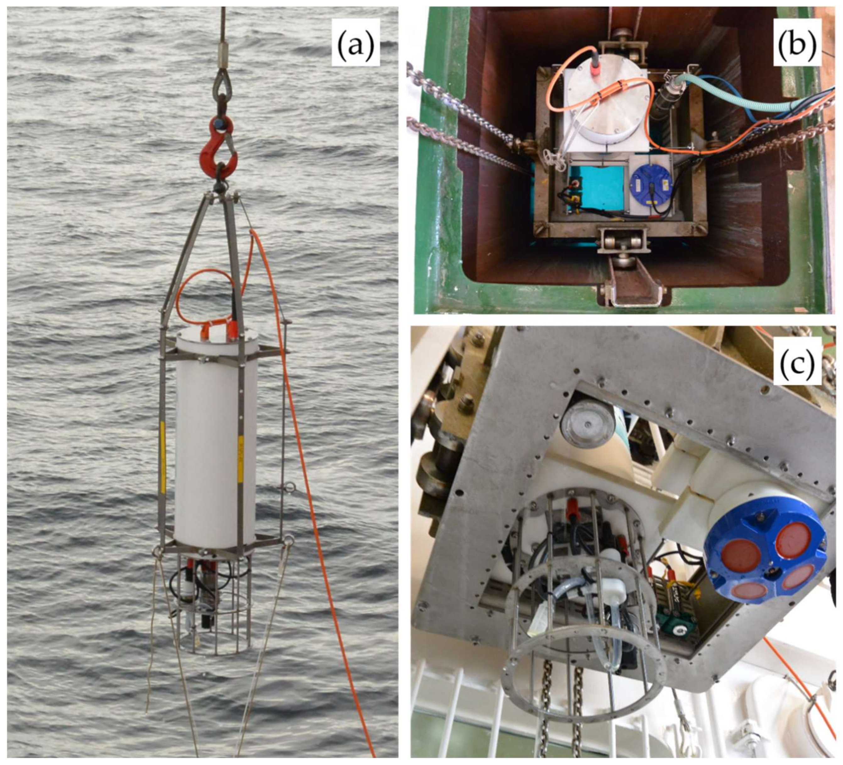
Figure 1 shows the deployment of the EEMS sensor system in profiling mode (
Figure 1a) and the deployment in a moonpool of a research vessel for in situ underway investigations (
Figure 1b,c). The submersible design offers automated data acquisition from water samples to a maximum water depth of 200 m in a freely selectable time interval, without the support of an operator. Once installed, autonomous long-term investigations from days to weeks are possible, depending on biofouling [
35] of the optical sensor unit and sediment load of the water filtration unit.
2.1.2. EEMS Sensor System Design and Technical Implementation
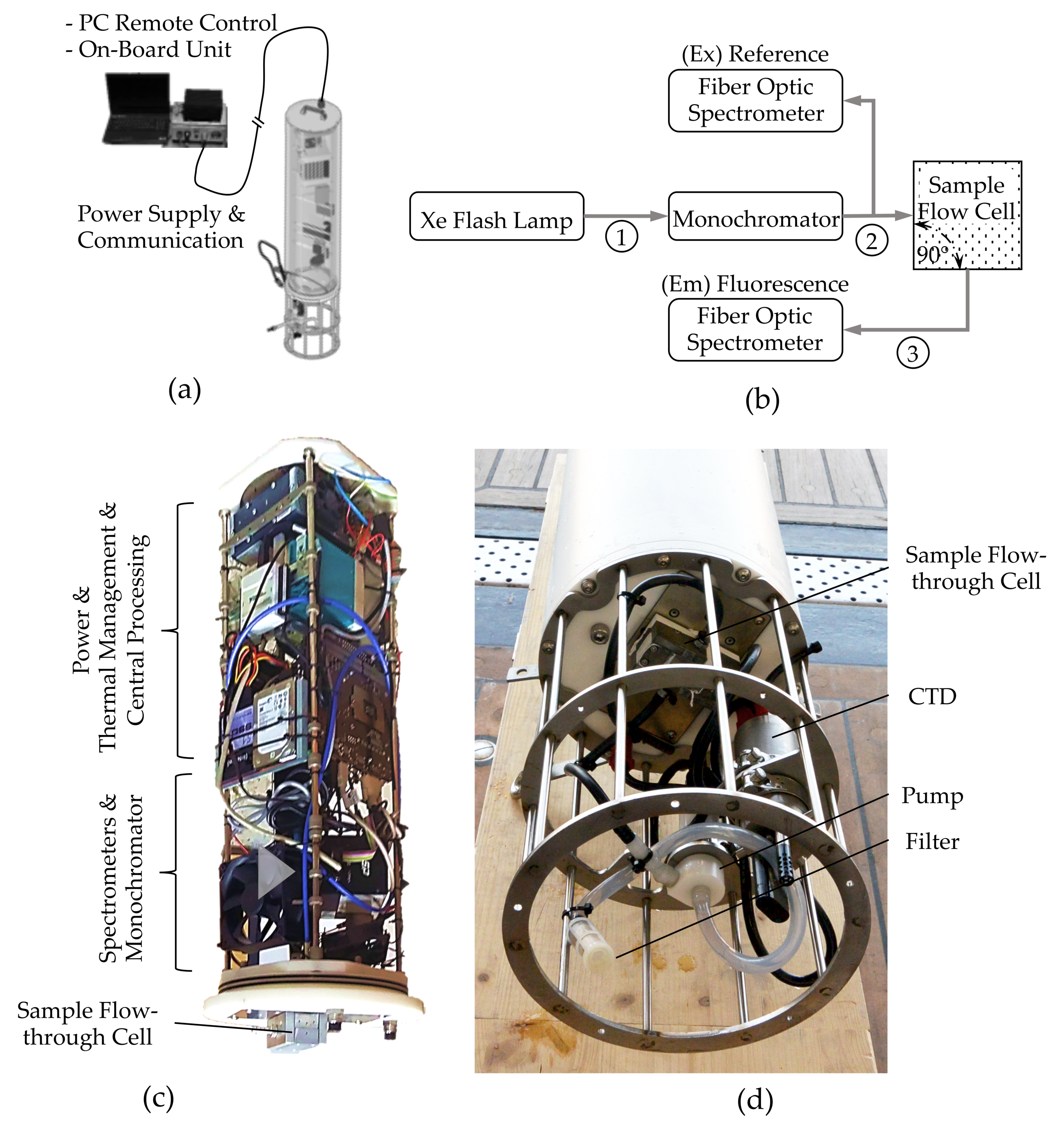
The entire EEMS sensor system is designed for a stand-alone operation as an underwater unit that only needs to be supplied with electrical power from an external power source. In this way, a moored operation with an external 12 V DC battery pack can also be realized. In case of shipborne installations like profiling or underway measurements, the system can be connected to an on-board unit via a 200 m seaworthy cable, as illustrated in
Figure 2a. The on-board unit provides 130 V DC power supply and data transmission to the ‘Kallemeter’ via Ethernet. This gives the opportunity to connect an external PC for remote control of the underwater unit, automatic data backup, or real-time visualization of the in situ measurements. In addition to the in situ fluorescence spectrometer unit, the ‘Kallemeter’ was equipped with a turbidity meter (STM/bh, Seapoint Sensors Inc., Exeter, NH, USA) and a CTD (Conductivity, Temperature, Depth) (miniCTD probe, ASD Sensortechnik GmbH, Trappenkamp, Germany). The ‘Kallemeter’ housing is made of a solid PEEK (polyether ether ketone) tube with steel plates at its ends, which also support the dissipation of thermal energy to the aquatic environment through internally forced convection, as this is important to provide long-term stability of the measurement system (light source and optical measurement devices). The EEMS sensor system is controlled through an integrated Microsoft Windows 7 PC, digital I/O converters, and LabVIEW software (version 2013, National Instruments, Austin, TX, USA), using a custom-made control program (named ‘EEMsea’). The latter allows for comprehensive adjustments of the measurement procedures, like EEM wavelengths or control of the sampling interval. All EEM datasets are stored in a comma-separated value (CSV) file format and include system- and sampling-relevant metadata in the header (e.g., sampling-identifier, internal temperature, and coefficients), which are assigned to the standardized file structure from PerkinElmer Luminescence Spectrometers ([Info], [Setup], [SampleInfo], [SampleData]; PerkinElmer, Waltham, MA, USA). Therefore, postprocessing and statistical analysis of EEM spectra can easily be applied by standard third party software or Matlab Toolboxes (The MathWorks, Natick, MA, USA) e.g., for PARAFAC [
27].
The entire EEM fluorescence spectrometer design, which is presented in
Figure 2b, consists of the following fluorescence measurement components: In the fluorescence excitation strand, a Xenon flash lamp (PX-2, Ocean Optics, Largo, FL, USA) is used as a broadband light source, which is coupled to a monochromator (CM 110, Spectral Products, Putnam, CT, USA) via an optical fiber (1). The output of the monochromator is coupled via an optical Y-fiber (2) to the reference spectrometer (USB2000+, Ocean Optics, Largo, FL, USA). Through this, a reference measurement of the excitation spectrum is realized. In parallel, the optical Y-fiber (2) connects the monochromator output to a flow-through sample cell in which the sample medium is located. The fluorescence emission strand consists of the detection spectrometer (QE-Pro, Ocean Optics, Largo, FL, USA) coupled via an optical fiber (3) to the sample flow-through cell. In the following, details of the fluorescence measuring system and its components are presented.
Fluorescence Excitation Light Source
Some in situ sensor designs use Xenon flash (or pulsed) lamps due to their high energy output in the ultraviolet (UV) and visible regions of the light spectrum as well as their long lifespan [
36]. For these reasons, the ‘Kallemeter’ also utilizes a Xenon flash lamp (PX-2, Ocean Optics, Largo, FL, USA), which emits pulsed light with a continuous spectrum in a fluorescence relevant excitation wavelength range from 220 nm to 750 nm. A pulse power of maximum 45 microjoules/pulse (with 5 µs pulse duration at 1/3 height of pulse) and a lifetime of 10
9 pulses are expected for this ‘expendable part’ (estimated 230 days continuous operation @ 50 Hz pulse rate). A stable output from pulse to pulse is guaranteed for up to 100 Hz repetition rate, so the flash delay results in 10 milliseconds. Since the total intensity typically decreases slowly over the operating period [
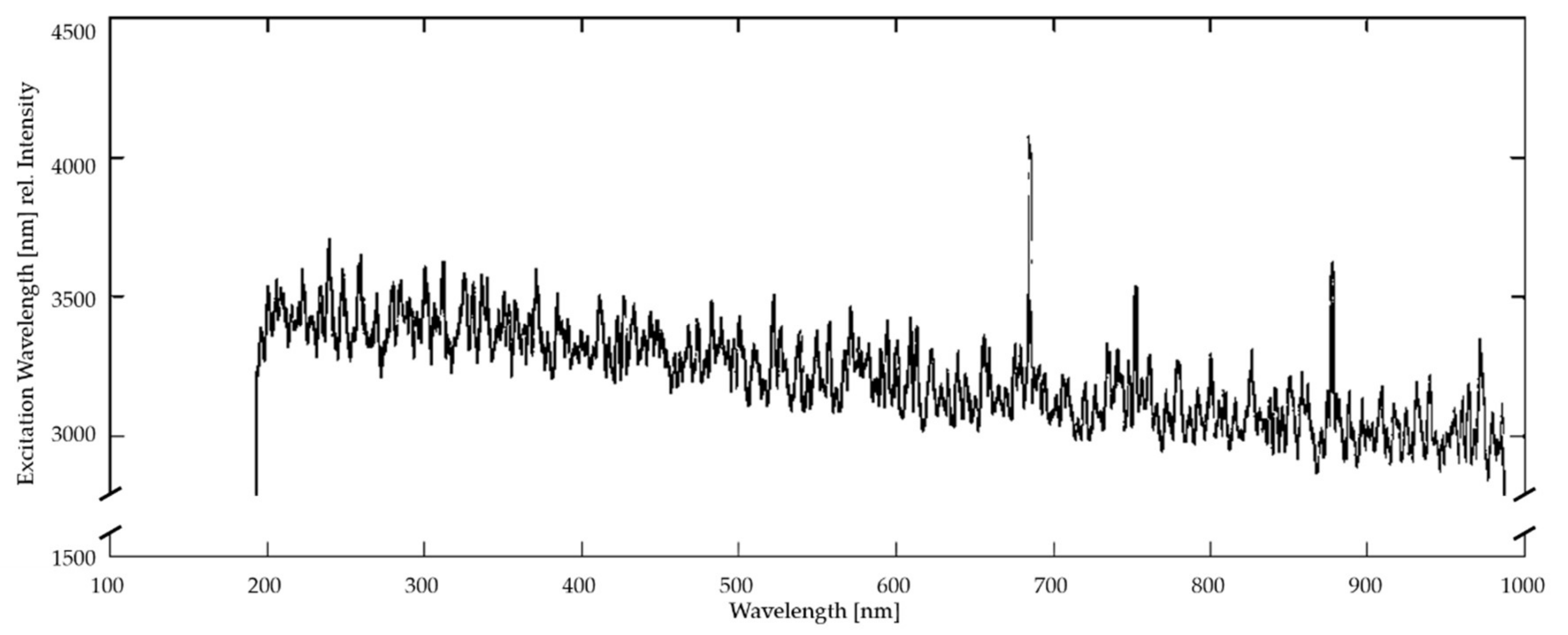
37], a measurement of the excitation spectrum is implemented to provide metadata of the EEMS sensor system status (presented in the subsection “Quality status of the excitation wavelengths”).
Control of the Fluorescence Excitation Band
A monochromator (Type CM 110, Spectral Products, Putnam, CT, USA) is used to separate a narrow excitation band from the spectrum of the Xenon flash lamp. A full width at half maximum (FWHM) effective bandwidth of 10 nm is realized (therefore no slits are used) and the excitation wavelengths are selectable from 200 nm to 750 nm in 1 nm steps (with ruled grating AG1200-00300-303). The monochromator provides a coupling and decoupling angle of 14.8° and results to 0.13 numerical aperture (NA).
Quality Status of the Excitation Wavelengths
A wavelength-calibrated reference spectrometer (USB2000+, Ocean Optics, Largo, FL, USA) controls the quality status of the excitation. The internally used grid provides a spectral sensitivity range from 200 nm to 800 nm with a fixed slit width of 100 μm, and a possible integration time from 1 millisecond to 65 s. Reference data are recorded in parallel to the fluorescence measurements but are not included in the calculation of the EEM spectra. Instead, they only serve as metadata for monitoring the quality of the excitation light source state over the operation time.
Water Sampling Flow-Through Cell
Various conceptual instrument designs and principles for fluorescence detection hardware are available for different applications: right angle detection, intersecting cones, flow-through, and fiber optic designs [
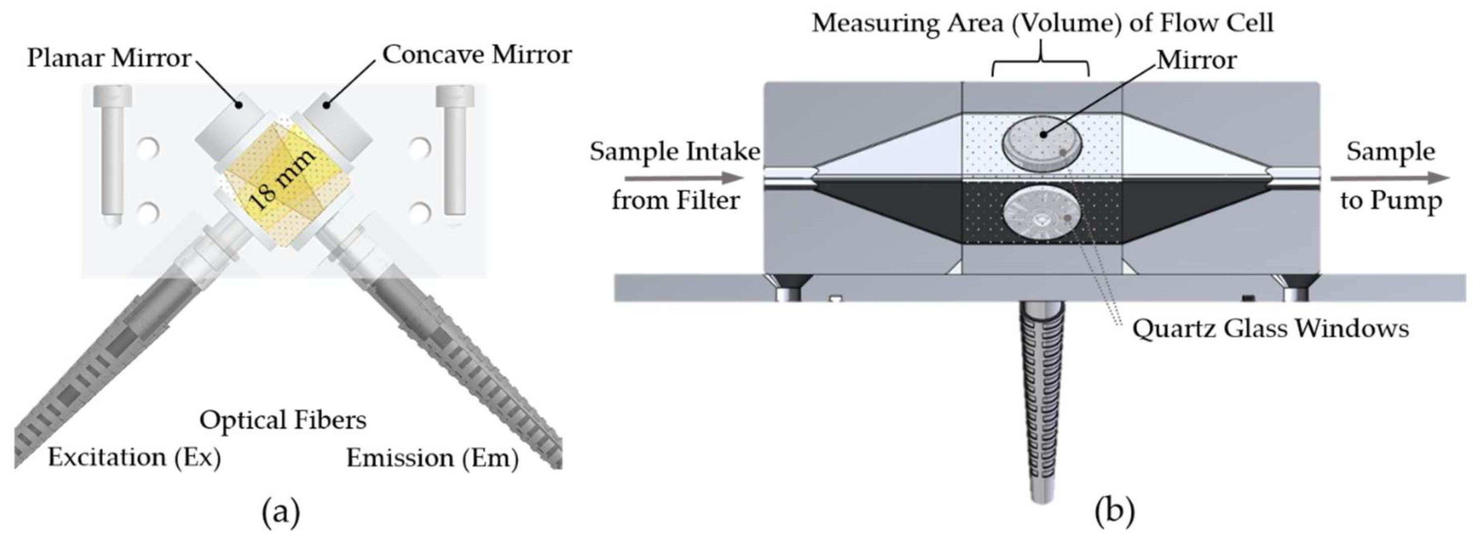
36]. The ‘Kallemeter’ sample flow-through cell design combines right angle detection (the commonly used 90° emission–excitation setup in luminescence spectrometry) with fiber optics and intersecting cones in a closed flow-through design, which is illustrated in
Figure 3a. In addition, the measuring cell makes use of well-directed multireflective intersections of the optical fiber aperture to achieve multiple excitations and detection cone overlaps. Thus, the optical path within the water sample is enhanced and an effective increase of factor 2.5 of the fluorescence signal for the highest signal-to-noise ratio can be achieved (
Appendix A,
Table A1). Two mirror elements are used for this purpose, which are arranged opposite to the optical fiber terminations in a way that no direct fluorescence excitation light can enter in the optical fiber of the detector strand. A concave mirror (CM127-025-F01 - Ø1/2” UV Enhanced Al-Coated, f = 25.0, Thorlabs, Newton, NJ, USA) is used in (opposite) combination to the excitation cone. With a focal length of 25 mm, the focus point of the selected concave mirrors is almost at the end of the optical fibers distance of 22 mm. A planar mirror (PF05-03-F01 - Ø1/2” UV Enhanced Al-Coated, Thorlabs, Newton, NJ, USA) is used in (opposite) combination to the emission cone of the optical fibers.
As the sample cell forms the contact point between the optical parts and the water sample, it is installed in a separate housing at the bottom of the EEMS sensor system (see
Figure 2c,d). Thus, a decoupling of the fluid-carrying and pressurized parts from the sensitive internal structures of the measurement unit is achieved and a simple sealing and pressure tightness can be realized. The optical interfaces of the sample cell, which are in contact with a seawater sample, are covered with superior transparent quartz glass windows (#45-310. TECHSPEC, Ø 15 mm Uncoated, 1λ Fused Silica Window, Edmund Optics, Barrington, NJ, USA). In order to ensure biogeochemical inertness of the sample cell, a specific adhesive (LS2-6140, NuSil Technology, Carpinteria, CA, USA) was selected through in situ tests as a suitable material for connecting the sample cell components and quartz windows. Even after several days in aqueous solution, this adhesive did not emit any fluorescent substances.
The flow-through geometry type results in a greater efficiency in signal output compared to an open-faced design. Thus it is a good choice for waters with a wide range of NOM concentrations and low numbers of particles, as the sensor geometry (sample volume) is well defined [
36]. A closed flow-through cell design, as illustrated by the cut-section in
Figure 3b, provides shading of the optical inner parts from ambient light. This is a further benefit for an in situ application as it reduces the effect of biofouling [
38]. During the sampling process, the closed sample cell is flushed with the water sample. The inlet side of a mini submersible pump for profiling applications (SBE 5M-1, Sea-Bird Scientific, Bellevue, WA, USA) is connected to the water outlet of the sample cell, while a reusable 50-μm nylon screen filtration element (type series F20 filter housing, Wolftechnik Filtersysteme, Germany) is connected to the sample cell water inlet via opaque hoses. This prevents an uncontrolled exchange between the ambient water and the water sample volume during an EEM spectrum measurement. This is particularly important for in situ underway operations when the ‘Kallemeter’ moves through different water bodies during an ongoing EEM measurement. Note that the setup presented herein was not equipped with a 0.2 µm or 0.45 µm filter, as recommended to separate the dissolved from the particulate fraction of organic matter. This is also the case for common bulk fluorescence sensors, as used in this study for comparison. However, as a pumped flow-through system, the ‘Kallemeter’ is generally capable of such a filtration unit as used e.g., for in situ spectral absorption measurements of CDOM [
17].
Main Fluorescence Detector
The main fluorescence detector unit of the ‘Kallemeter’ EEMS sensor system is a wavelength-calibrated CCD digital spectrometer with a high dynamic range of ~85.000:1 (QE-Pro, Ocean Optics, Largo, FL, USA). The fluorescence emitted by the water sample is transmitted via an optical fiber, which is installed at the sample flow-through cell. The spectrometer built-in grating enables the detection in a full range of emission wavelengths from 200 nm to 950 nm, which corresponds to the detection range of commonly used laboratory luminescence spectrometers (e.g., the LS55, PerkinElmer, Waltham, MA, USA). The slit of the detector spectrometer has a width of 100 μm. Long-term stability and noise reduction is achieved by internal Peltier cooling of the detector to −10°C, as all fluorescence measurements signals are subject to alterations as a function of temperature. Temperature changes can arise either from self-heating of the instrument or from changes in ambient temperature of the deployment environment. Integration times of 8 milliseconds up to 60 min are selectable to enable stable measurements for environments where sample signal intensity is small. The spectrometer includes further a second order wavelength filter, preventing detection of Rayleigh and Raman scattering of higher orders.
The chosen detector spectrometer offers automatic dark measurements without external shutter units, which is used to obtain related metadata to correct for instrument response variables. As a routine by the ‘EEMsea’ software, a dark count measurement is carried out once initially per EEM spectrum measuring cycle and is automatically subtracted from the fluorescence data. Investigations of wavelength assigned intensity dark count measurements are presented in
Appendix A,
Figure A1 through a long-term measurement test (116 h) exhibiting stable operating conditions with no drift or significant invariance over time.
Optical Fibers
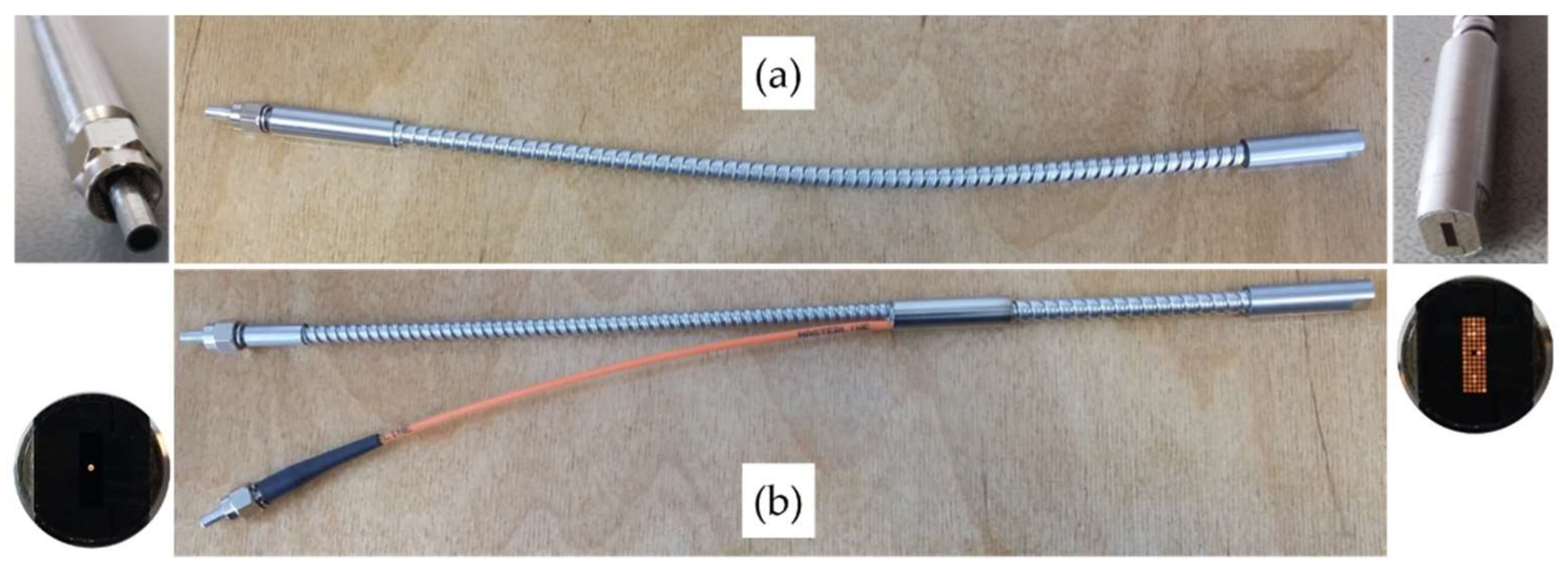
Optical fibers in the system setup are solarization-resistant, as ultraviolet radiation below 260 nm degrades transmission in silica fibers, also known as UV degradation. The custom-made designs, as illustrated in
Figure 4a, provide maximum fiber diameters (80 single fibers 200 μm core diameter, Ø 2.6 mm bunch, LOPTEK, Berlin, Germany) and achieve a high transmission (96%) in all relevant excitation wavelengths (labeled (1) in
Figure 2b). The numerical aperture is NA = 0.22.
Figure 4b shows the optical Y-fiber and the single 80 µm fiber to the reference spectrometer that measures the reference excitation spectrum (labeled (2) in
Figure 2b). This constellation prevents super-saturation or even damage of the reference spectrometer. For the fluorescence emission (detection) strand, a conventional optical fiber is used (QP1000-2-UV–Vis, Ocean Optics, Largo, FL, USA), connecting the sample flow-through cell to the main fiber optic spectrometer (labeled (3) in
Figure 2b).
2.1.3. EEMS Sensor System Fluorescence Performance Evaluation
As the complete ‘Kallemeter’ EEMS sensor system is based on a new design, the system performance for wavelength calibration, fluorescence intensity and signal-to-noise ratio was examined prior to field application. Considering the main focus of this article being the field application, the most important facts and a compilation of regularly practiced calibration methods for the in situ EEMS sensor system will be presented in the following section. All settings for the following measurements are listed in detail in
Table A2 of the
Appendix A.
The general procedure to calibrate an in situ fluorometer consists of (i) precalibration with tests of pressure, mechanical, and electronic stability as well as precision, (ii) signal output calibration to measure the dark and maximum counts, (iii) internal temperature calibration, (iv) determination and record of offset values with purified water at different temperatures, and (v) manufacturer calibration to obtain the scale factor of the fluorometer [
36]. Calibration should be repeated in regular intervals, because environmental conditions can vary and lamp as well as spectrometer performance can degrade over time.
Table 1 summarizes the EEMS sensor system specifications.
Signal-To-Noise Ratio
The signal-to-noise ratio (S/N) of the Raman band of tap water is easy to realize and a widely used method to quantify the sensitivity of a spectrofluorometer [
39,
40]. The S/N (where S denotes signal intensity and N noise intensity) of the Raman band is calculated with the following equation.
For the ‘Kallemeter’ a S/N of 34 was determined for the Raman band measurement of tap water as presented in
Figure A2.
Wavelength Calibration
The wavelength calibration of the EEMS sensor system needs no special adjustments by the user, as both spectrometers used are calibrated by the manufacturers and therefore are supplied with a set of calibration coefficients. For verification we performed a laboratory check with a reference standard for molecular fluorescence spectrophotometry (Compound 610; excitation: 440 nm; emission: 480 nm; nominal concentration of 1 × 10⁻⁶ M, Starna Scientific Ltd., Ilford, UK), data not shown. Such a measurement allows the evaluation of the EEMS optical setup over time and corresponding correction methods for the emission wavelengths.
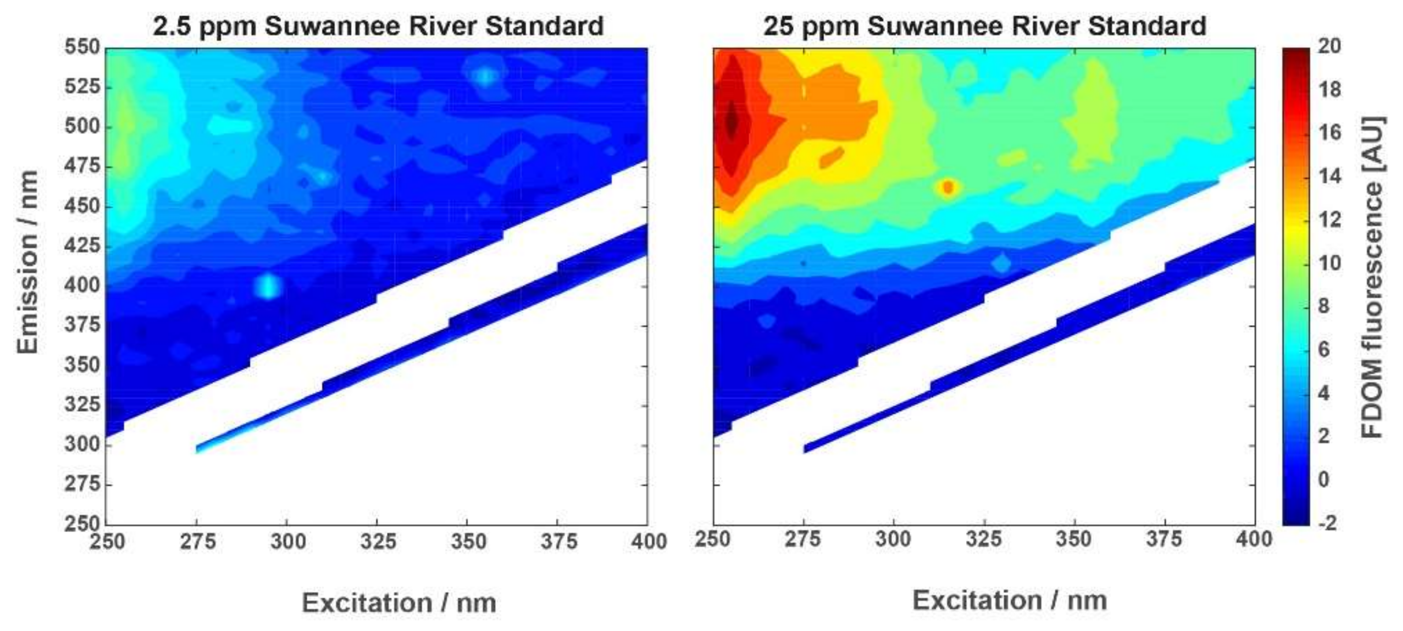
Intensity Calibration with Suwannee River Standard
Since 1982, representatives of the International Humic Substance Society (IHSS) have isolated reference fulvic acids, humic acids, and natural organic matter (NOM) from the Suwannee River in southeastern Georgia, USA. Suwannee River has a remarkable low variance in its elemental composition and is therefore a commonly accepted standard. It has a long history as reference material for multidisciplinary research areas, including the marine community [
41]. For the fluorescence measurement of the ‘Kallemeter’, a sulfuric acid dilution of Suwannee River (sample charge number 2S101H) was used with concentrations of 2.5 ppm and 25 ppm. The EEM spectra of the two concentrations of Suwannee River standard are shown in
Figure 5. Receiving reasonable signal intensity in both samples indicated sufficient signal intensity for nominal concentrations at marine study sites.
2.2. FerryBox-Based Organic Matter Fluorescence Measurements
An important step in the evaluation of the ‘Kallemeter’ is the comparison with other existing sensors and approaches, here with two commercially available sensors, the Cyclops-7-U (Turner Designs, San Jose, CA, USA) and the MatrixFlu-UV (TriOS, Rastede, Germany) mounted in a FerryBox system (4H-JENA engineering, Jena, Germany) installed on the ship during the research cruise (see
Section 2.3). Furthermore a LS-55 spectrofluorometer (PerkinElmer, Waltham, MA, USA) was used as a common standard for laboratory measurements (see
Section 2.4), providing complete EEM spectra directly comparable with the ‘Kallemeter’. The FDOM sensors either provide only certain parts of the full EEM (MatrixFlu-UV) or only bulk fluorescence data (Cyclops-7-U).
As described previously [
43], there are two versions of the MatrixFlu sensor, one for the visible wavelengths, with a focus on phytoplankton, and one for the ultraviolet, dedicated to FDOM components. The latter is used here and referred to as MatrixFlu-UV. The fundamental idea is to measure the typical peaks of organic matter fluorescence, as described by Coble [
29], instead of assessing the whole excitation and emission spectrum, thus enabling a rapid detection and a high temporal resolution. This section describes only the sensor’s main features, as its technical design has been published elsewhere [
23,
44].
The MatrixFlu-UV sensor consists of an excitation light source with distinct wavelengths combined with a set of detectors collecting a near field emission of a fluorescence signal at certain wavelengths directly in the water column (open sensor interface). Each combination of an excitation and emission wavelength results in a different fluorescence channel. The optical part contains a single semiconductor device emitting light at three different wavelengths (254 nm, 280 nm, and 320 nm) on the same optical axes. Four single semiconductor detectors are arranged around it collecting the fluorescent signal in an angle of approx. 170° to the optical axes. Different wavebands are selected via customizable narrow bandwidth filters (here 280 nm, 360 nm, 460 nm, and 540 nm). By doing this, all possible combinations result in twelve different channels.
FDOM components referred to in this work are mainly associated to (a) terrestrial or old marine humic-like substances (peak C), (b) “freshly produced” marine humic-like substances (peak M), and protein-like Tryptophan substances (peak T) [
45,
46]. Humic components show a further related excitation maxima for UV light of higher energy (lower wavelength) but same emission position or range (peak A) [
45]. Data from all MatrixFlu-UV channels are collected simultaneously. For the comparison with the ‘Kallemeter’ and the other bulk fluorescence sensor (described below), Channel 11 was extracted and evaluated, corresponding to peak C (EX/EM 320 nm/460 nm). Data was averaged on every minute values and smoothed by a moving mean filter (window size 13). Factory calibration and further information about the sensor performance are available in [
23].
The Cyclops-7-U sensor estimates bulk FDOM concentration by measuring the fluorescence emission at 470 nm (60 nm peak width) for an excitation at 325 nm (120 nm bandwidth filter [
47]). Thus, for a comparison with the data from this sensor, the ‘Kallemeter’ in situ EEM signal in the area corresponding to an excitation of 265 to 385 nm and an emission of 440 to 500 nm have been integrated. This provides a ‘Kallemeter’ derived bulk fluorescence signal that corresponds to the excitation and emission ranges given in the specifications of the Cyclops-7-U sensor.
2.3. FerryBox Installation and Other Oceanographic Parameters Measured
The water intake of the FerryBox was realized in the moonpool of the research vessel (in approx. 4 m depth) close to the measuring head of the submersed ‘Kallemeter’ to ensure a comparability of the measurements between the three types of instruments. Besides the FDOM data, readings of standard oceanographic parameters, such as temperature, salinity, and chlorophyll a fluorescence were also obtained. All FerryBox data were averaged on minutely values and smoothed by a moving mean filter (window size 11).
2.4. FDOM Laboratory Water Samples
Sampling from the near surface water, here defined as the samples collected between 0.1 and 2.0 m, was obtained with a submersible pump system and stored in 5 L white plastic bottles, at all stations. Samples were filtered in the laboratory immediately after sampling, and stored at 4 °C in previously rinsed glass bottles. CDOM absorption and EEM spectra measurements were completed within 24 h after sampling.
Samples were filtered with a glass syringe device through GF/F Nucleopore filters (0.2 μm, GE Healthcare Whatman, Piscataway Township, NJ, USA). CDOM absorbance spectra were obtained between 220 and 650 nm at 5 nm intervals on a Shimadzu UV-2550PC UV–VIS spectrophotometer (Shimadzu, Kyoto, Japan) with 10 cm quartz cuvettes. All measurements were performed at room temperature using freshly produced ultrapurified water (UPW; Milli-Q 185plus water purification system, Merck Millipore, Burlington, MA, USA) as reference. CDOM absorption was calculated by multiplying absorbance by 2.303/r, where r is the cuvette length (in meter). FDOM EEM spectra measurements were conducted at room temperature on a LS55 spectrofluorometer (PerkinElmer, Waltham, MA, USA) equipped with a Xenon flash lamp, pulsed at line frequency of 60 Hz. The excitation (EX) and emission (EM) scanning ranges were set to 200 to 400 nm (5 nm interval) and 220 to 550 nm (0.5 nm interval), respectively. The scanning speed was 1200 nm min
−1, the EX and EM slit was set to 10 nm, and the detector gain was at medium range (775 V). Daily measurements of UPW were used as references. Water Raman scatter peaks were eliminated by subtracting the EEM spectra of UPW blanks. Inner filter effect and Rayleigh scatter peaks were corrected using the drEEM toolbox [
33]. Lamp variations were normalized to the Raman peak integral (EX: 350 nm) using freshly produced UPW, therefore producing normalized intensities in Raman units (RU) [
39]. EEM spectra were resized due to high S/N in certain regions. Therefore, excitation wavelengths below 250 nm and emission wavelengths below 300 and above 550 nm were excluded from the subsequent PARAFAC modeling process.
PARAFAC modeling was performed with the drEEM toolbox (ver.0.2.0) in MATLAB R2015b (The MathWorks, Natick, MA, USA) according to a method described previously [
33], employing the N-way toolbox as the engine of the PARAFAC algorithm [
34]. A three-component model was validated by split-half analysis, random initialization analysis, and residuals analysis. The model explained up to 99.95% of the variability within the lab-based LS55 spectrofluorometer EEM dataset.
A similar PARAFAC analysis was applied on the Kallemeter-based EEM spectra along cruise track between station 11 and 15. Correction for inner filter effects was realized by utilizing the measured absorption spectra from the nearest station and using Kallemeter blank measurements from an initial laboratory test with purified water. Four out of 48 spectra were excluded from the analysis, due to high residual error and leverage load, validating a two-component model that explained up to 61% of the variability within the dataset through split-half analysis, random initialization analysis, and residuals analysis. A third component could not be detected.
2.5. Study Site
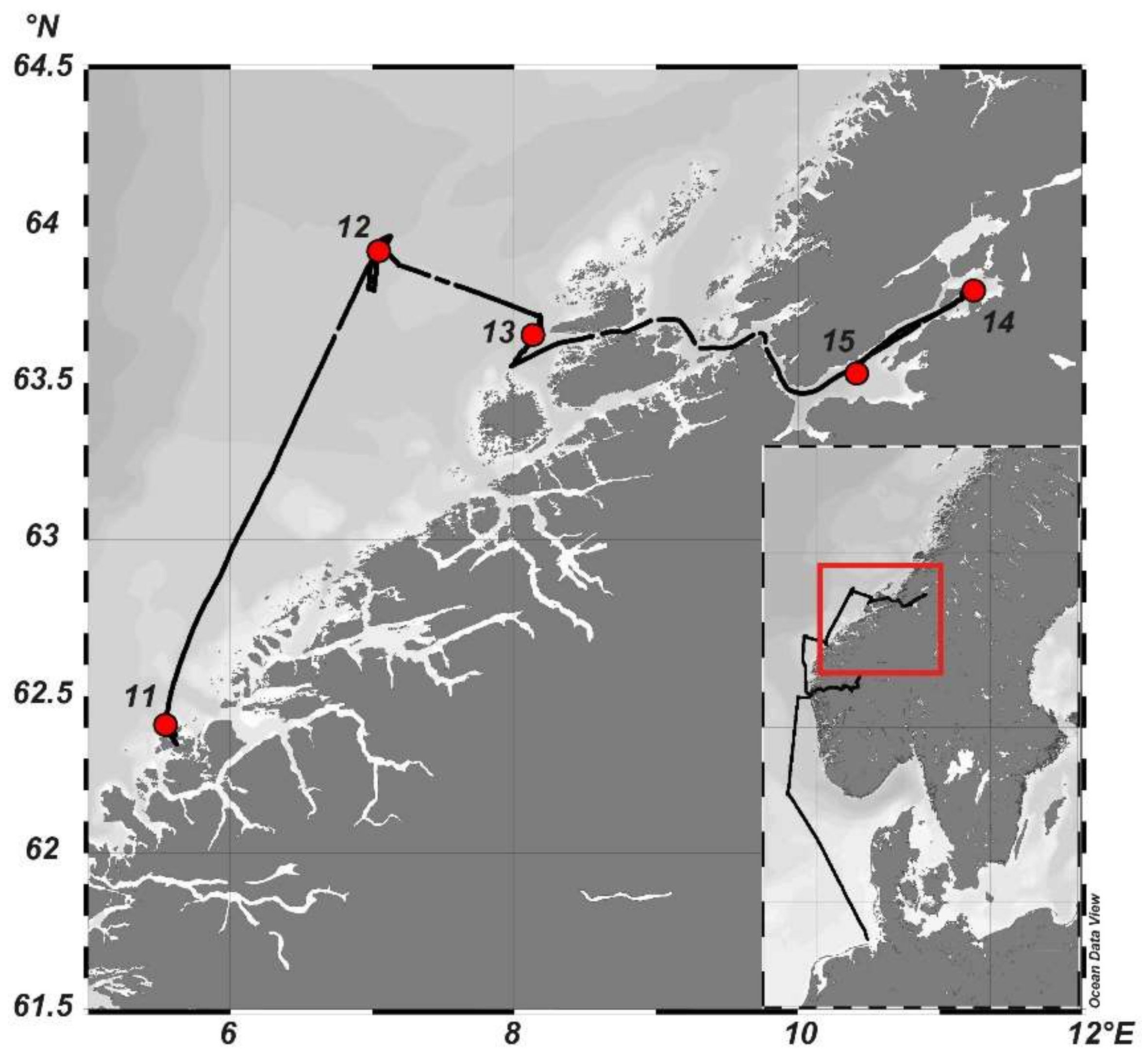
In order to assess the performance of the ‘Kallemeter’ in comparison with the MatrixFlu-UV and the FerryBox-mounted Cyclops-7-U fluorescence sensors in the field, the data obtained during an expedition (HE491) with research vessel R/V Heincke from the coastal sea into the Trondheimsfjord (Norway) were analyzed.
Figure 6 shows a map of the study site and the cruise track investigated. The instruments were in parallel operation from 19th to 25th of July 2017. The Trondheimsfjord is the third-largest fjord in Norway with a length of 140 km, a volume of 235 km
3, and a surface area of 1420 km
2. It is divided in three basins and has a seaward sill depth of 195 m [
48]. It is characterized by comparably high CDOM concentrations as well as vertical and horizontal gradients [
49], making it an ideal test site.
3. Results
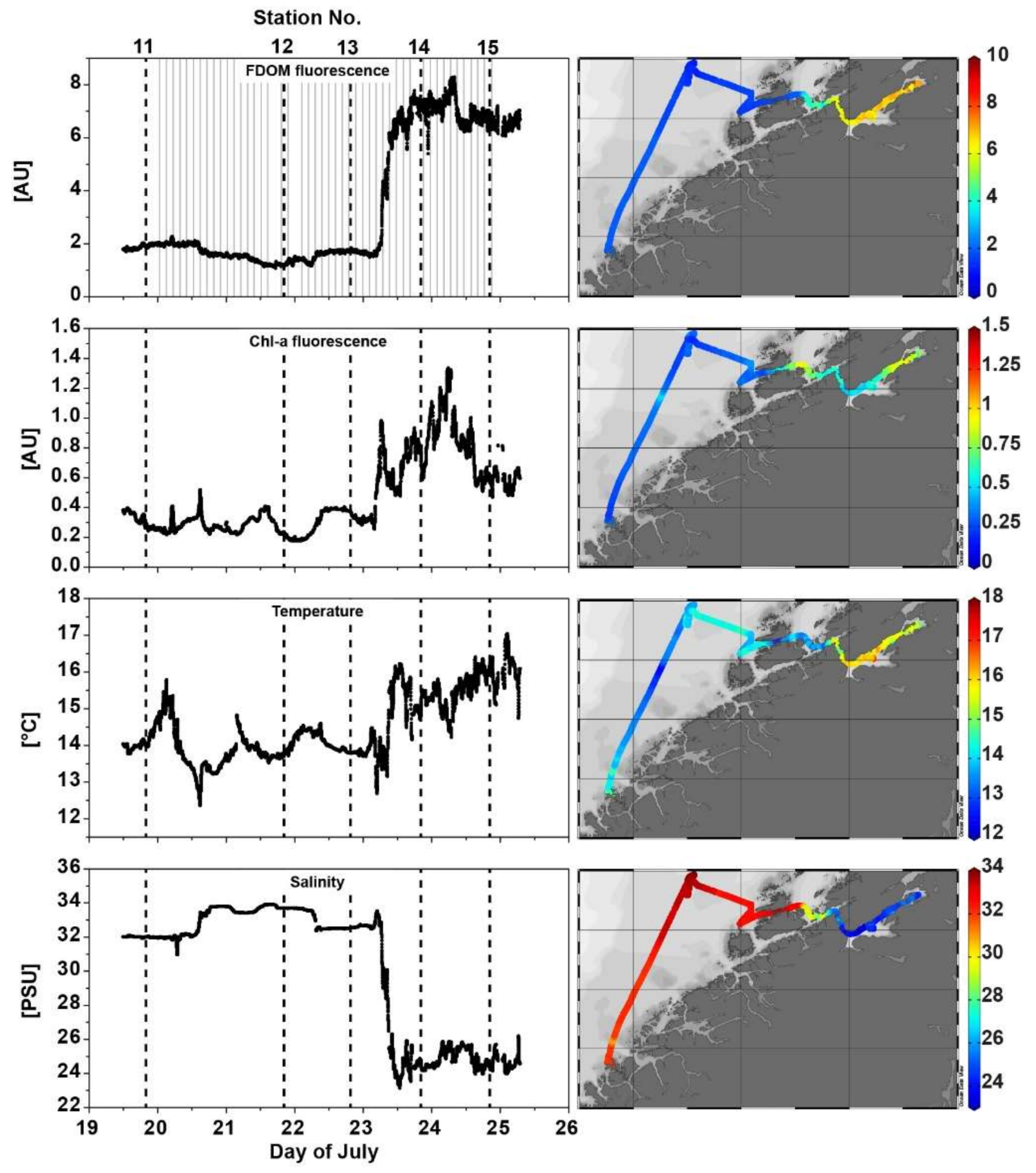
The FerryBox data is well suited to provide a first overview of the overall fjord hydrography. The FerryBox dataset started on 19 July in the Norwegian coastal sea (station 11) heading first northwards (station 12) and then into the Trondheimsfjord (station 13), through the mid-fjord section and towards the innermost part of the fjord (station 14). From there, the transect went back to the mid-section and ended at station 15 on 25 July. There is a considerable difference in all parameters measured between the area outside and within the fjord (
Figure 7), indicating the presence of two water bodies with different properties. With the exception of salinity, values of all parameters are higher within the fjord. Salinity is highest towards the ocean side, with values of more than 32, rapidly decreasing inside the fjord towards the mid-section exhibiting values of around 24. Temperature increases slightly from around 14 °C in the outer section towards 15 to 17 °C in the mid- and inner-part of the Trondheimsfjord. Chlorophyll-a fluorescence (here provided in AU, as the sensor has not been specifically calibrated for chl-a before the cruise) shows a gradual increase from the seaward part of the fjord to a maximum at the end of the fjord. FDOM from the Cyclops-7-U fluorometer (provided in AU) shows, inverse to salinity, a four-fold increase and steep gradient from the seaward side of the fjord towards the mid- and inner-part.
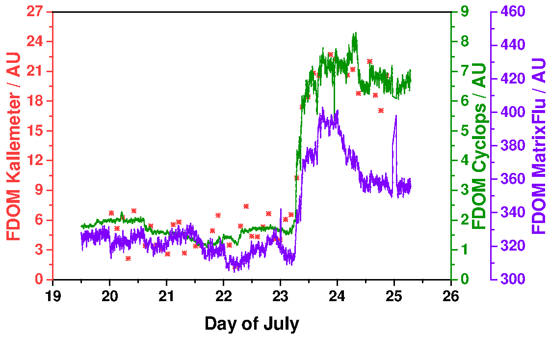
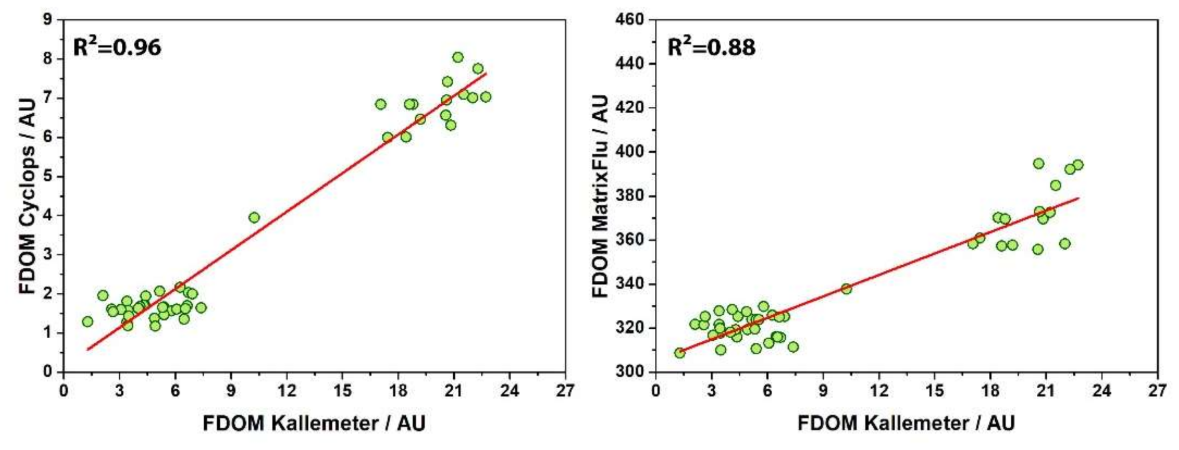
Comparing the ‘Kallemeter’ bulk fluorescence signal extracted from the EEM spectra against the bulk fluorescence signal of the MatrixFlu-UV channel 11 and the FerryBox inbuilt Cyclops-7-U FDOM sensor data (
Figure 8), it can be seen that all three signals showed a steep increase on 23 July, when entering Trondheimsfjord. MatrixFlu-UV exhibited a maximum at the end of that day, followed by a decrease on 24 July towards a steady level around half of the signal range. FDOM bulk fluorescence from the FerryBox inbuilt Cyclops-7-U sensor increased in the same steep way towards a higher level on 23 July. Signal intensity stayed on this level with only a slight decrease in the morning of 24 July. ‘Kallemeter’ bulk fluorescence signal, as indicated by red stars, exhibited the same dynamical behavior as the Cyclops-7-U. A linear regression analysis was performed (
Figure 9) of the extracted ‘Kallemeter’ bulk fluorescence against the Cyclops-7-U sensor (coefficient of determination R
2 = 0.96) as well as the corresponding channel of the MatrixFlu-UV (R
2 = 0.88), both attached to the flow through system.
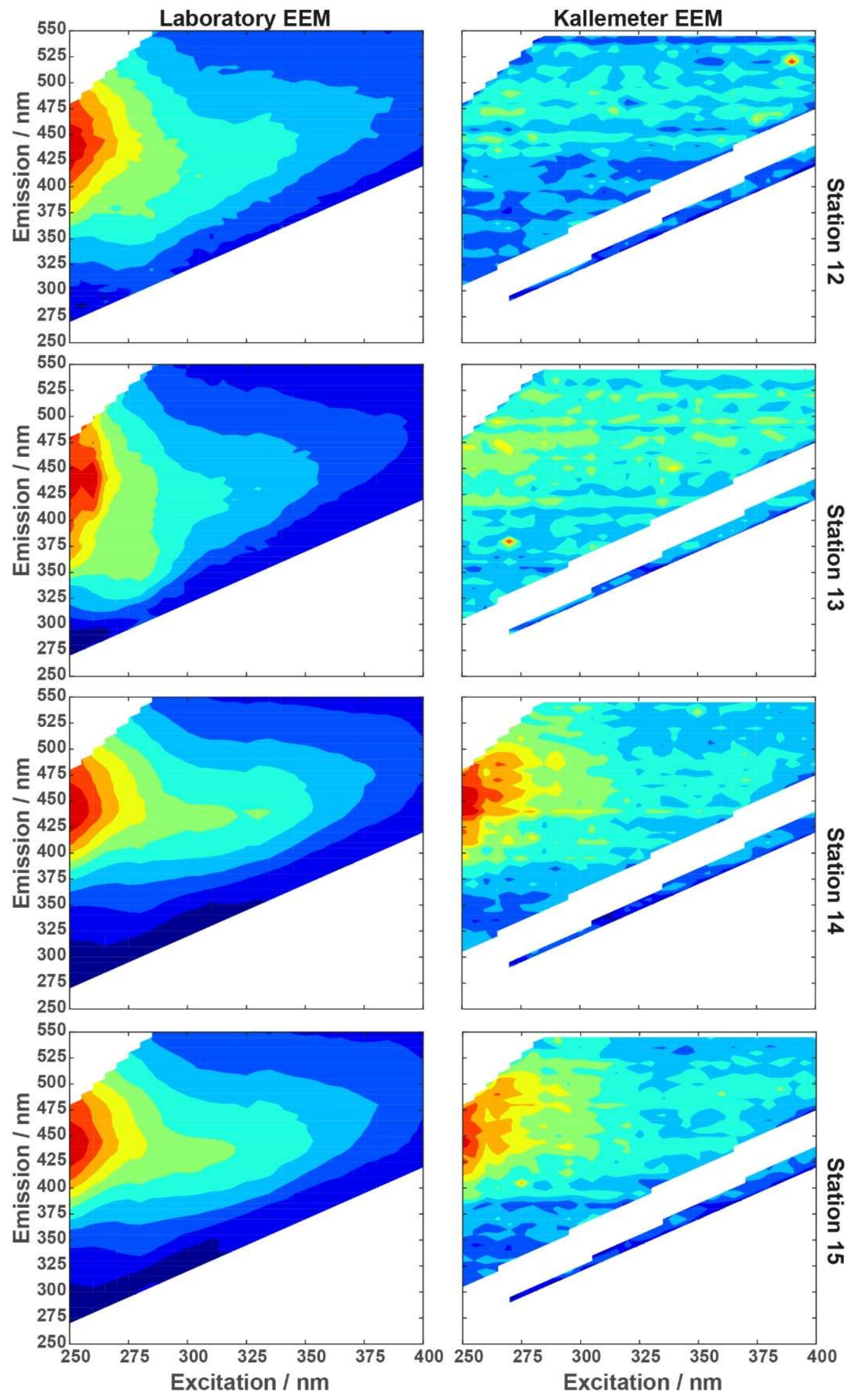
In situ underway EEM measurements, measured by the ‘Kallemeter’ in the moonpool of R/V Heincke, provided a total of 48 spectra in 5 days (20 to 25 July). All fluorescence information and metadata were continuously recorded from open water into the Trondheimsfjord. A comparison of normalized EEM spectra of the lab-based LS55 fluorometer with the corresponding nearest normalized Kallemeter-based EEM spectra at stations 12–15 (
Figure 10; station 11 had no close match-up within a time frame of ±1 h) shows good similarity for stations 14 and 15, where signal intensities are 5-times higher as compared to stations 12 and 13 (compare
Figure 8). These lower concentrations of fluorescent organic matter at stations 12 and 13 were only resolved from the apparently more sensitive laboratory LS55 spectrofluorometer, thus illustrating the current limits of the ‘Kallemeter’ with respect to low concentrations and the effects of noise. Please note that we applied normalization to the EEM spectra to enable a comparison of spectra signatures measured, independent from the signal strength. A non-normalized set of ‘Kallemeter’ EEM spectra is provided in the appendix (
Figure A3) showing for every fourth dataset (a) an EEM spectra with EX wavelengths 230–550 nm, Δλ = 10 nm, integration time of 60 s and two averaged scans, slit = 10 nm, EM wavelengths 189–990 nm, and (b) an emission scan with EM wavelengths 189–990 nm for 250 nm EX wavelength. These Kallemeter-based EEM spectra show an increase in fluorescence intensities inside Trondheimsfjord as compared to the coastal water conditions in the EM wavelength range from 400 to 550 nm.
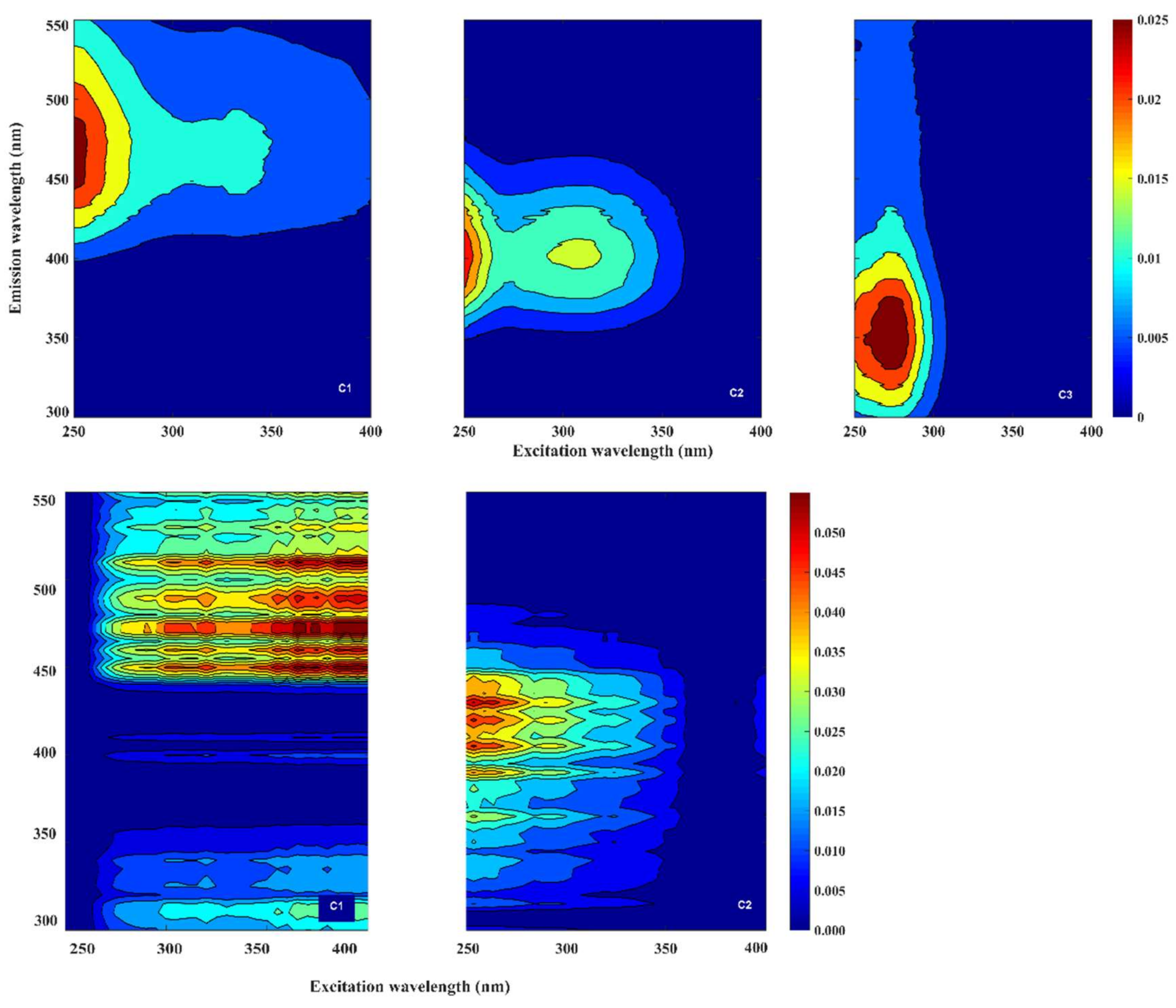
PARAFAC analysis of the lab-based LS55 spectrofluorometer EEM spectra from water samples gathered at different depths demonstrated the presence of three main components (C1, C2, and C3) in the water samples (
Figure 11, top panel). These components were characterized by their excitation and emission pairs (EX/EM) as follows. Component (C1) corresponding to terrestrial humic-like peaks A
C and C, component (C2) corresponding to marine humic-like peaks A
M and M, and component (C3) corresponding to protein-like Tryptophan peak T, as suggested by Coble [
29]. The spectral composition of the recorded lab-based LS55 spectrofluorometer EEM spectra (provided in
Table 2) shows that the fluorescent intensity of the peaks C1, C2, and C3 remains constant between the open ocean stations (ST11 and ST12) and the outer section of the fjord (ST13). Once the mid- and inner-part of the fjord was reached, we recorded a sharp increment (by a factor of 5) in the fluorescent intensity for the components C1 and C2 (ST14 and ST15), while C3 stays nearly constant.
Performing PARAFAC analysis of the Kallemeter-based EEM spectra along the transect resulted in a model with two components validated (
Figure 11, bottom panel). These components, even though influenced by the noisy EEM spectra that suited as model dataset, can be related according to their excitation/emission pairs to the presence of terrestrial humic-like peaks A
C and C, and marine humic-like peaks A
M and M. Although reasonable EEMS where produced by the ‘Kallemeter’, the presence of noise and suspended materials in the samples must be addressed in the future, in order to minimize the observed displacement on the peak’s position.
4. Discussion, Limitations, and Conclusions
The main objective of this study was to present a novel in situ EEMS sensor system—the ‘Kallemeter’—enabling full optical fingerprints in a submersible design. We presented the design of this system within the methods
Section 2.1 and illustrated its application based on laboratory samples of diluted Suwannee River standards with 2.5 ppm and 25 ppm, respectively. Fluorescence exhibited around EX: 240 nm and EM: 450 nm was corresponding to terrestrial humic-like peak C substances, as expected for Suwannee River standards, with increasing intensity and additional visible contributions extending to higher excitation wavelengths [
50,
51]. The assessment of the ‘Kallemeter’ EEMS sensor systems’ signal-to-noise ratio (S/N) based on the Raman peak of water in a tap-water sample, provided an S/N of 34. Compared to commercially available laboratory spectrofluorometers that exhibit S/N of 500 or higher the ‘Kallemeter’ is much more limited in resolving low signal intensities [
39]. Part of this is based on the different optical components implemented, e.g., a fiber optic spectrometer compared to a monochromator plus photomultiplier setup for the LS55 spectrofluorometer, still considered as the gold-standard for high sensitivity applications. Also the choice of the excitation light was influenced by power- and heat-considerations and therefore restricted to <10 Watts, where other laboratory instruments like the Aqualog (Horiba, Kyoto, Japan) are equipped with up to 150 Watt Xenon flash lamps [
52]. The strongest influence can be assumed from the application of fiber optics within the sensor, resulting in losses while coupling light in and out as well as transmitting it in the fiber. The use of fiber optics is a result of the compact design that a submersible housing requires—a potential redesign of the ‘Kallemeter’ will take this into account and try to partially avoid the use of optical fibers through direct light paths.
The field application of the ‘Kallemeter’ was realized in the moonpool of R/V Heincke on transect from Norwegian coastal waters into the Trondheimsfjord in July 2017. The system was successfully operated for five days in a fully submerged installation. EEM spectra derived from this application showed very low fluorescence intensities superimposed by noise components for all coastal sea measurements and the outer fjord area, while mid- and inner-fjord measurements exhibited clear broad signals of approximately EX: 250–300 nm and EM: 400–500 nm. These observations are consistent with the spectral component intensities derived from laboratory UV–VIS spectrofluorometer (LS55, PerkinElmer, Waltham, MA, USA) measurements of surface water samples. With respect to components C1 and C2 derived from PARAFACS analysis these were ranging for the outer fjord between 0.02 and 0.04 Raman Units, while mid- and inner-fjord values ranged between 0.09 and 0.18 RU. The direct comparison of normalized EEM spectra from the lab-based spectrofluorometer and the ‘Kallemeter’ (
Figure 10) illustrated both, the capability of the ‘Kallemeter’ to provide full EEM spectra if fluorescent organic matter concentrations are sufficiently high (stations 14 and 15), and the limitation to resolve low concentrations against the background noise as encountered at stations 12 and 13 in coastal waters. The latter is a result of the lower S/N and sensitivity, discussed above. The application of the ‘Kallemeter’ EEMS sensor system in its current form therefore seems to be limited towards areas with an increased amount of fluorescent organic matter, typically encountered in near coastal areas, estuaries and inland waters. Furthermore a study of the impact of noise or signal degradation applied on EEM spectra that serve as PARAFAC model input would be of interest to assess general limitations, however that is beyond the scope of this study.
The PARAFAC analysis of the Kallemeter-based EEM spectra enabled us to model two components, corresponding to terrestrial humic-like peaks AC and C, and marine humic-like peaks AM and M. This was compared to a PARAFAC analysis of the LS55 spectrofluorometer EEM spectra from near surface water samples at the distinct stations that successfully validated three components. While lab-based components 1 and 2 resemble the in situ Kallemeter components (even though limited by high noise influence), the third component, namely the protein-like Tryptophan peak T, could not be reproduced from the ‘Kallemeter’ data. Since peak T could be quantified in the laboratory measurements to an average intensity of 0.023 Raman units without any signal increase in the Trondheimsfjord, we consider this as a current limitation for the ‘Kallemeter’.
The ability to perform a PARAFAC analysis on automatically measured in situ EEM spectra is a major achievement and, to the best of our knowledge, the first of its kind. We encountered a couple of challenges to that end, that we provide here as current limitations but also avenues for future improvements. (A) Since we did not filter the water entering the measurement cell with 0.2 µm (only applying 50 µm to keep coarse material out) the signal observed is originating from dissolved, colloidal and particulate fractions of organic matter. For low amounts of particulate material this might not be a problem and indeed all in situ FDOM bulk fluorescence sensors (including the two used in this study for comparison) are also measuring unfiltered samples. However, for direct comparison with laboratory measured (filtered) FDOM EEM spectra this can be considered an obstacle. To overcome this, the installation of a filter unit at the inlet, containing an appropriate 0.2 µm filter can be easily realized in future applications of the ‘Kallemeter’. It can be speculated that part of the noisiness of the spectra and PARAFAC components can be associated to the influence of particulate material. (B) All EEM spectra need to be corrected for the inner filter effect (IFE). This typically requires a parallel measurement of the absorption spectra of the filtered water sample over the same wavelength range. The ‘Kallemeter’ itself is not suited to perform this absorption measurement, therefore we applied absorption spectra from water samples analyzed with a laboratory spectrophotometer. These were only available at the five stations investigated and not at the 48 measurement locations of the ‘Kallemeter’. Assigning absorption spectra from samples that were gathered up to 24 h earlier or later is introducing uncertainties, even though we took care to respect the different oceanographic gradients encountered in the matching procedure. A much better way to account for this need of parallel absorption measurements will be to use automated in situ capable methods [
53]. (C) Applying mirrors in the sample flow through cell, we increased the fluorescence signal intensity by a factor of 2.5, however IFE corrections applied to correct EEM spectra do not consider these and are therefore overcorrecting. Luciani et al. [
54] showed how mirrors change the fluorescence signal and can be at the same time utilized to correct for IFE, if measurements with and without mirrors are performed on the same sample. This could be another methodological improvement to overcome constraints mentioned above.
Comparing the results from the bulk fluorescence signal of the ‘Kallemeter’ (calculated from the EEM spectra) with the flow through data from the commercially available FDOM sensors (a) inside the FerryBox (Cyclops-7-U, Turner Design, San Jose, CA, USA) and (b) the channel 11 from the recently developed matrix fluorescence sensor (MatrixFlu-UV, TriOS, Rastede, Germany), a good correspondence could be observed. The maximum exhibited on 23 July and the following decrease in the ‘Kallemeter’ fluorescence intensity (compare
Figure 8) seems to be better reproduced by the Cyclops-7-U FDOM sensor. The corresponding MatrixFlu-UV channel is able to reproduce the same steep increase, however shows a signal reduction afterwards, not represented by the other methods applied in this study. As this study reports one of the first field datasets achieved with the MatrixFlu-UV sensor we cannot judge on this readings but see a clear need to investigate the sensors responses.
The MatrixFlu-UV sensor was investigated herein only with respect to one of its 12 channels representing a main spectral component in the investigated environment. It is therefore herein utilized as single-channel sensor and its further value in rapid quasi-EEM spectra measurements will be investigated in future works. Other multichannel approaches exist, with two [
55] or three [
56] combinations technically built up from single EX/EM combinations. A recent study of Nordic seas FDOM intensities [
57] utilized a novel three-channel fluorometer (WETStar, Sea-Bird Scientific, Bellevue, WA, USA). This system excites the water sample in a flow-through cell with two LEDs at 280 nm and 310 nm. Two detectors measure the emission at 350 nm and 450 nm, allowing for a combination of channels in specific peak areas: peak C (with EX/EM 310 nm/450 nm), peak A
C (with EX/EM 280 nm/450 nm), and peak T (with EX/EM 280 nm/350 nm). All applications mentioned above underline the potential of multichannel FDOM measurements for specific components dominant in natural water bodies. The technological step from multichannel sensing to real excitation–emission matrix spectroscopy with high spectral resolution in both, the excitation and the emission sides, is huge, since it requires complete different technologies. An interim step with six (up to 12) distinct LED excitation wavelengths and emission spectra with 7.5-nm spacing (named ‘LEDIF’) was presented as part of a field-deployable optical system [
58].
The ‘Kallemeter’ represents, to the best of our knowledge, the first submersible EEMS sensor system that performs full optical fingerprints. While the detection side is comparable to the LEDIF approach, using a fiber optical spectrometer, excitation was realized in our system by a Xenon flash lamp and an embedded controlled monochromator. This enabled us to achieve 10-nm steps in the excitation wavelengths selection (and finer steps are technically feasible); however, it also slows down the measurement process to approx. 30 min per individual sample. This is in the same order of magnitude as the LS55 (PerkinElmer, Waltham, MA, USA) UV–VIS laboratory spectrofluorometer used in this study. Faster laboratory systems exist nowadays (e.g., Aqualog, Horiba, Kyoto, Japan) that enable EEM spectra measurements below 5 min that require, however, further technical improvements (e.g., a TE cooled back-illuminated CCD fluorescence detector, and a high power Xenon flash lamp). Modern ocean observing strategies combine sensors with high spatiotemporal resolution but limited information depth with more sophisticated sensors, that provide a high depth of information but are limited in their spatial and temporal resolution [
8]. The ‘Kallemeter’ is one of those highly sophisticated sensors and will likely, as others in that field [
59,
60], improve in its operational specifications, i.e., size, weight, and power. Multichannel fluorescence sensors for FDOM are already smaller, lightweight, and less power consuming. Their application on different autonomous platforms has been demonstrated [
17,
55,
58]. Thus, they are the linkage towards resolving rapid changes and processes. An assessment of fluorescent organic matter in high spatiotemporal and spectral resolution is therefore technically feasible and likely to become standard in future biogeochemical ocean observatories.

 ,
, 


