A Brief Review of Mueller Matrix Calculations Associated with Oceanic Particles

Featured Application

This paper provides guidance for selecting an appropriate method for calculating the Mueller matrix associated with oceanic particles of arbitrary morphologies and refractive indices.

Abstract

The complete Stokes vector contains much more information than the radiance of light for the remote sensing of the ocean. Unlike the conventional radiance-only radiative transfer simulations, a full Mueller matrix-Stokes vector treatment provides a rigorous and correct approach for solving the transfer of radiation in a scattering medium, such as the atmosphere-ocean system. In fact, radiative transfer simulation without considering the polarization state always gives incorrect results and the extent of the errors induced depends on a particular application being considered. However, the rigorous approach that fully takes the polarization state into account requires the knowledge of the complete single-scattering properties of oceanic particles with various sizes, morphologies, and refractive indices. For most oceanic particles, the comparisons between simulations and observations have demonstrated that the “equivalent-spherical” approximation is inadequate. We will therefore briefly summarize the advantages and disadvantages of a number of light scattering methods for non-spherical particles. Furthermore, examples for canonical cases with specifically oriented particles and randomly oriented particles will be illustrated.

1. Introduction

It is well known that the scattering of light by a particle is determined by the detailed characteristics of the scattering particle, particularly its size, chemical composition (thus, the index of refraction), the overall shape, and detailed surface texture (e.g., surface roughness). Oceanic particles vary greatly in size and morphology. While the Lorenz-Mie theory has been used frequently to simulate the optical properties of oceanic particles (e.g., [1,2,3,4,5]), these particles are predominately nonspherical. Significant differences exist in the optical properties simulated by using “equivalent” spheres and non-spherical shapes, such as spheroids (e.g., [6]). In addition, even the simplest biological cell has a membrane and plasma contained within the membrane. Previous studies have shown that accounting for the cell structure can better simulate the optical properties of various phytoplankton species, particularly the scattering at large scattering angles [5,7,8,9,10,11]. Advanced light scattering methods have been developed to deal with complex shape and structure. Here, we briefly summarize light-scattering computational methods for oceanic particles. Light scattering in an absorbing medium has been extensively discussed [12,13,14]. For generality, however, only a nonabsorbing medium is discussed here. Beginning with Maxwell’s equations, in Section 2, we will show exact volume-/surface-integral equations for mapping the near field to the far field. Furthermore, we introduce both the amplitude scattering matrix and the scattering phase matrix. In Section 3, several scattering methods will be introduced. In Section 4, discussions are given that are based on oriented particles and particles in random orientation.

2. Fundamental Concepts for Mueller Matrix Calculations

2.1. Maxwell’s Equations and the Volume/Surface-Integral Equations

Since all of the rigorous light-scattering computational methods should obey Maxwell’s equations, we will first give a brief introduction to the role that both the volume/surface methods for mapping the near field to far field play in the final solutions. We will only consider time-harmonic electromagnetic waves and dielectric particles. The dielectric particles are assumed to be isotropic and have a linear response to an applied field. In this case, Maxwell’s equations in the medium while using SI units are as follows:

$$\nabla \stackrel{.}{·E}(\overrightarrow{r})=0,\nabla \times E(\overrightarrow{r})=-\mu \frac{\partial H(\overrightarrow{r})}{\partial t},$$

(1)

$$\nabla \stackrel{.}{·H}(\overrightarrow{r})=0,\nabla \times H(\overrightarrow{r})=\epsilon \frac{\partial E(\overrightarrow{r})}{\partial t},$$

(2)

where E and H are the electric and the magnetic fields, respectively; ε and μ are the permittivity and permeability of the medium. Using the Fourier transformation, an arbitrary incident field in the time-domain can be transformed into the summation of the fields in the frequency-domain, or the time-harmonic fields. Assuming that the time-harmonic field follows exp(−iωt), where ω is the angular frequency of the electromagnetic wave, Maxwell’s equations in a time-independent form become:

$$\nabla \stackrel{.}{·E}(\overrightarrow{r})=0,\nabla \times E(\overrightarrow{r})=i\omega \mu H(\overrightarrow{r}),$$

(3)

$$\nabla \stackrel{.}{·H}(\overrightarrow{r})=0,\nabla \times H(\overrightarrow{r})=-i\omega \epsilon E(\overrightarrow{r}).$$

(4)

Using Equations (3) and (4), the vector Helmholtz equations for the electric and magnetic fields are

$$\left({\nabla }^2+k^2\right)E(\overrightarrow{r})=0,$$

(5)

$$\left({\nabla }^2+k^2\right)H(\overrightarrow{r})=0,$$

(6)

where k is the wave number and k² = ω²με. For oceanic particles, the surrounding medium and the scattering particles are assumed to be nonmagnetic, thus μ = μ₀, where μ₀ is the vacuum permeability. The light speed c in vacuum is equal to $1/\sqrt{{\mu }_0{\epsilon }_0}$, where ε₀ is the permittivity in vacuum. Consequently, the refractive index m of the medium is $m=c/v=\sqrt{\epsilon /{\epsilon }_0}$, where $v$ is the light speed in the medium. Since the electric and the magnetic fields are dependent on each other, we will use the electric field to describe the electromagnetic field.

The volume integral and surface integral equations of the electric field can be deduced from Maxwell’s equations and the vector Green function [15]. In the far-field regime, they can be expressed in the form

$${E^{\mathrm{sca}}(\overrightarrow{r})|}_{r\to \infty }=\frac{\exp (ikr)}{-ikr}\frac{i{k}^3}{4\pi }{\displaystyle \underset{V}{\int }{d}^3{\overrightarrow{r}}^{\prime }\left\{(m^2-1)\left[\widehat{r}\times \widehat{r}\times E(\overrightarrow{r}\prime )\exp (-ik\widehat{r}·\overrightarrow{r}\prime )\right]\right\}},$$

(7)

$${E^{\mathrm{sca}}(\overrightarrow{r})|}_{r\to \infty }=\frac{\exp (ikr)}{-ikr}\frac{k^2}{4\pi }\widehat{r}\times {\displaystyle \underset{S}{\oint }{d}^2\overrightarrow{r}\prime \left\{\left[{\widehat{n}}_s\times E(\overrightarrow{r}\prime )\right]-\frac{\omega {\mu }_0}{k}\widehat{r}\times \left[{\widehat{n}}_s\times H(\overrightarrow{r}\prime )\right]\right\}},$$

(8)

where the parameters are given in Figure 1; ${\widehat{n}}_s$ is the outward normal to the surface. It is evident that the scattered far field only depends on the scattered directions with an outgoing spherical wave factor exp(ikr)/kr.

2.2. Amplitude Scattering Matrix and Mueller Matrix

Let the incident direction of the incoming wave be along the z-axis of the laboratory frame of reference. The incident direction and the scattered direction define a scattering plane and the incident and scattered fields can be expanded into parallel and perpendicular components with respect to the scattering plane. Consequently, the amplitude scattering matrix S can be given by [16]

$$\left(\begin{array}{l}{\mathrm{E}}_{\parallel }^{\mathrm{sca}}\\ {\mathrm{E}}_{\perp }^{\mathrm{sca}}\end{array}\right)=\frac{\exp (ikr-ikz)}{-ikr}S\left(\begin{array}{l}{\mathrm{E}}_{\parallel }^{\mathrm{inc}}\\ {\mathrm{E}}_{\perp }^{\mathrm{inc}}\end{array}\right),$$

(9)

where ${\mathrm{E}}_{\parallel }^{}$ and ${\mathrm{E}}_{\perp }^{}$ denote the parallel and perpendicular components of the electric field with respect to the scattering plane and S is a 2 × 2 complex matrix. The Stokes parameters in a non-absorbing medium are defined based on the measurable quantities, which are normally expressed in terms of a four-element column vector, the Stokes vector I, as follows:

$$I=\left(\begin{array}{c}\mathrm{I}\\ \mathrm{Q}\\ \mathrm{U}\\ \mathrm{V}\end{array}\right)=\left(\begin{array}{c}{\mathrm{E}}_{\parallel }{\mathrm{E}}_{\parallel }^{*}+{\mathrm{E}}_{\perp }{\mathrm{E}}_{\perp }^{*}\\ {\mathrm{E}}_{\parallel }{\mathrm{E}}_{\parallel }^{*}{-\mathrm{E}}_{\perp }{\mathrm{E}}_{\perp }^{*}\\ {\mathrm{E}}_{\parallel }{\mathrm{E}}_{\perp }^{*}+{\mathrm{E}}_{\perp }{\mathrm{E}}_{\parallel }^{*}\\ i\left({\mathrm{E}}_{\parallel }{\mathrm{E}}_{\perp }^{*}{-\mathrm{E}}_{\perp }{\mathrm{E}}_{\parallel }^{*}\right)\end{array}\right).$$

(10)

In the above equation, i is the imaginary unit and a constant factor, $\sqrt{\epsilon /{\mu }_0}/2$, is neglected since usually relative quantities are measured. The Mueller matrix (also called the scattering phase matrix in the literature) is the transformation matrix from the incident to the scattered Stokes parameters, as follows:

$$I^{\mathrm{sca}}=\frac{1}{{(kr)}^2}P{I}^{\mathrm{inc}},$$

(11)

where the 4 × 4 Mueller matrix P can be given as quadratic expressions of the amplitude scattering matrix S, as follows [17,18]:

$$P=A\left(S\otimes S^{*}\right)A^{-1},$$

(12)

where asterisk denotes the complex conjugate and symbol $\otimes$ denotes the tensor product, and the constant matrix A is

$$A=\left(\begin{array}{cccc}1& 0& 0& 1\\ 1& 0& 0& -1\\ 0& 1& 1& 0\\ 0& i& -i& 0\end{array}\right),A^{-1}=\frac{1}{2}{A}^{†},$$

(13)

in which the symbol † (sometimes called the dagger) is composed of two operations; namely, complex conjugating (the * symbol), and then transposing the original matrix and the order of these operations is unimportant. Note that the Stokes parameters have the units of irradiance [19], and on the other hand, the corresponding radiance is invariant over distance if no scattering or absorption occurs.

If the incident light is unpolarized, the scattering cross-section can be given in terms of the element P₁₁ by

$$C_{\mathrm{sca}}=\frac{1}{k^2}{\displaystyle \underset{4\pi }{\int }d\mathsf{\Omega }{\mathrm{P}}_{11}(\theta ,\phi )}.$$

(14)

The phase function is defined as:

$$p=\frac{4\pi }{k^2{C}_{\mathrm{sca}}}{\mathrm{P}}_{11},$$

(15)

and the scattering phase matrix can be defined as:

$$F=\frac{4\pi }{k^2{C}_{\mathrm{sca}}}P.$$

(16)

The symmetry relations of the phase matrix have been extensively discussed in general and also for forward and backward scattering [20,21,22]. For an arbitrary particle without mirror symmetry in the scattering plane, the scattering phase matrix of a particle in random orientation is in the form

$$F=\left(\begin{array}{cccc}{a}_1& b_1& b_3& b_5\\ b_1& a_2& b_4& b_6\\ -b_3& -b_4& a_3& b_2\\ b_5& b_6& -b_2& a_4\end{array}\right),$$

(17)

where there are only 10 independent parameters. For a particle with mirror symmetry in the scattering plane, the scattering phase matrix of a particle in random orientation is reduced to a block-diagonal matrix, as follows:

$$F=\left(\begin{array}{cccc}{a}_1& b_1& 0& 0\\ b_1& a_2& 0& 0\\ 0& 0& a_3& b_2\\ 0& 0& -b_2& a_4\end{array}\right),$$

(18)

where there are only six independent parameters. Equations (17) and (18) represent the scattering phase matrix of a particle in random orientation. For a collection of particles with a size distribution, the collective scattering phase matrix can also be defined in terms of the distribution and the reader is referred to the book by Mobley [23].

All of the scattering quantities have been presented and we are now faced with the problem of obtaining the near fields or directly the far fields satisfying Maxwell’s equations.

3. General Scattering Method for Suspended Particles

The governing principle for light scattering by particles is Maxwell’s equations. The scattering solution is called Rayleigh scattering if x « 1 and |mx|« 1 [16,20], where the size parameter x is defined as 2πr_v/λ with r_v being the radius of a sphere or volume-equivalent sphere and λ the incident wavelength in the surrounding medium. The analytical solutions to Maxwell’s equations are only effectively available for spheres [16,20]. For a prolate or oblate spheroid, the analytical solution is given in a series of the spheroidal wave functions by Asano and Yamamoto [24] and Asano and Sato [25]. However, the analytical solutions for a spheroid are only computationally effective for small particles due to numerical instability in computing the spheroidal wave functions for large particles. For an infinite circular cylinder, the analytical solution can be easily computed [16]. However, the infinite morphology does not exist in nature. For a particle with spherical symmetry, such as a homogeneous sphere or a multi-layered sphere, the analytical solution can be obtained by using the Lorenz-Mie theory for any size [16,20]. The advantage of using the spherical model is the computational efficiency, while the disadvantage is the appearance of spherical artifacts, such as the rainbow or glory, which have seldom been observed for ocean water (e.g., [26]). For a non-spherical particle, the solution of Maxwell’s equations consists of two categories: rigorous and approximate solutions. The rigorous solutions can be further divided into numerically exact solutions and semi-analytical T-matrix solutions.

3.1. Numerically Exact Methods

As the name implies, numerically exact solutions use numerical methods to directly solve Maxwell’s equations or the volume or surface integral equations derived from Maxwell’s equations. The computational precision depends on the numerical resolution.

The finite difference time-domain method (FDTD) is based on the discretization of Maxwell’s equation Equations (1) and (2) both in time and space [27]. The FDTD method uses the Yee grid to discretize the space, which was developed by Yee [28] and reviewed by Taflove [27], and Yang and Liou [29,30]. Since the computational space has to be confined to a finite region, a perfectly matched layer is used to absorb all of the electromagnetic waves in the computational boundary and avoid any artificially reflected electromagnetic waves back into the computational region [31]. The computational region usually with cuboid shape has to encompass the scattering particle so the computational region is always larger than the scattering particle in the FDTD application. The electromagnetic fields on the grids are updated with the advance of time so the FDTD is an initial value problem.

For a time-harmonic field or a field in the frequency domain, Maxwell’s equations become the vector Helmholtz equations that are given in Equations (5) and (6). The vector Helmholtz Equations (5) and (6) can be discretized in space while using the finite-element method (FEM) [32]. The boundary condition on the particle surface and the continuity condition on the neighboring grid give a series of linear equations. The FEM is a boundary value problem. A major challenge for applying the FEM to light scattering is choosing the finite region covering the scattering particle so that the field in the computational region satisfies the radiation condition in the far field [33]. Like the FDTD method, the computational region for the FEM is also larger than the region that is occupied by the scattering particle, which can constrain the application regime of the FEM.

Using the vector Green function, the differential equations become the volume-integral or the surface-integral equations given by Equations (7) and (8). Even though the volume-integral and the surface-integral methods are equivalent, the volume-integral method is numerically more stable than the surface-integral method because the volume-integral equation in Equation (7) is a Fredholm integral equation of the second kind whose matrix equation is usually diagonally dominant [34].

The discrete-dipole approximation (DDA) method is a typical volume-integral method. The DDA was first proposed by Purcell and Pennypacker [35] and it was reviewed by Draine [36,37] and by Yurkin and Hoekstra [38]. In the DDA method, the particle volume is discretized into usually cubic cells, as shown in Figure 2. Each cubic cell is represented while using an electric dipole and the excited field at that cell is composed of the original incident field and the field from all other cells but excluding the cell itself. The dipoles generate a series of linear equations and the fields with respect to all dipoles can be obtained by solving the corresponding linear equations. Once the total field with respect to each cell is obtained, the amplitude scattering matrix and Mueller matrix can straightforwardly be computed. It is evident from Equation (7) that the computational region is equal to the volume of a scattering particle. That makes the DDA method computationally efficient when compared to other numerically exact methods.

Two numerical implementations of the DDA are a FORTRAN implementation referred to as DDSCAT by Draine and Flatau [39] and a C implementation referred to as ADDA by Yurkin and Hoekstra [40]. The DDSCAT is parallelized for scattering only in different orientations so the memory requirement might restrict the computational capability for large particles. The ADDA is parallelized by distributing grids (dipoles) into different CPUs so the ADDA can handle particles of large sizes. The DDA method has been extensively used to simulate light scattering of oceanic particles. For instance, the light scattering of Emiliania huxleyi coccolithophore was simulated while using the DDSCAT by Gordon et al. [41] and using the ADDA by Zhai et al. [42]. Another example of the use of ADDA is the light scattering of dinoflagellates by Liu and Kattawar [43], where the chiral structure of the chromosomes is implemented by using discrete dipoles. This chiral structure leads to optical activity for certain dinoflagellates and another reason for measuring the complete single scattering Mueller matrix, which should be a fruitful area of research in remote sensing of the oceans.

The typical feature of a numerically exact method is that the error asymptotically approaches zero if the corresponding numerical grid that is associated with the method asymptotically reaches zero. Another feature for oceanic particles is that the convergence rate is much faster than the convergence rate of atmospheric particles because the relative refractive indices with respect to oceanic particles are close to unity. Moreover, the composition of a particle using the numerically exact methods can be arbitrary, homogeneous or inhomogeneous, or even different grid by grid.

For all of the numerically exact methods, the Mueller matrix is given in terms of the amplitude scattering matrix and they both depend on the incident direction. Consequently, the light scattering computation of a particle in random orientation while using these methods can usually be given by numerically summing the light scattering for different orientations. The convergence in the random orientation computation becomes significantly more difficult with increasing particle size so the computation will become time-consuming.

3.2. Semi-Analytical T-Matrix Method

The T-matrix method was originally proposed by Waterman [44,45]. The incident and scattered fields are expanded in a series of the vector spherical wave functions. The T-matrix connects the incident and scattered expansion coefficients because of the linearity of Maxwell’s equations. The T-matrix of a particle only depends on the intrinsic properties of the particle, such as the refractive index, morphology, and the orientation of the particle frame of reference and its origin location, but not on the incident state. Corresponding to Equations (7) and (8), the T-matrix can be obtained using the surface-integral and volume-integral methods. The computational method of the T-matrix based on the surface integral is called the extended boundary condition method (EBCM) or the null field method, and it was reviewed by Tsang et al. [46], Mishchenko et al. [47,48], Mishchenko and Travis [49], and Doicu et al. [50]. The T-matrix method based on the volume integral equation is called the invariant-imbedding T-matrix method (IITM) and it was originally proposed by Johnson [51]. The IITM was reviewed and developed by Bi et al. [52]. For a particle with axial symmetry, the T-matrix is decoupled into a block-diagonal form, so the computation is significantly simplified. The applications of the EBCM on spheroids, cylinders, and Chebyshev shapes are exceptionally effective [49]. However, when a particle has a large size or an aspect ratio far from unity or one that is asymmetric, the matrices in the T-matrix computation are often ill-conditioned. The T-matrix method that is based on the volume integral is much more stable than the EBCM because the volume integral equation in Equation (7) is a Fredholm integral equation of the second kind, which is often less ill-conditioned [34]. The extreme stability of the IITM has been validated by applying the IITM to particles with large sizes, extreme aspect ratios, or asymmetric particles [52,53]. For instance, the IITM were used to compute the light scattering of oceanic particles, such as Emiliania huxleyi coccoliths and coccolithophores by Bi and Yang [54], and diatoms by Sun et al. [11].

When compared to the numerically exact methods, the significant advantage of the T-matrix solution is the analytical realization for a particle with a random orientation. The computational time of T-matrix methods is usually shorter than the numerically exact methods because T-matrix methods use matrix inversion instead of iterations. Moreover, in contrast to the relatively large refractive indices of atmospheric particles, such as ice crystals (m ~ 1.33) and aerosols (roughly m > 1.5), the relative refractive indices of oceanic particles are usually smaller than 1.2. For this reason, using the T-matrix method for oceanic particles normally yields faster convergence and higher computational efficiency than for atmospheric particles. However, the computational time and memory requirements of the T-matrix are strongly related to the radius of the circumscribed sphere of a particle and its morphology. For instance, for a needle particle with small volume but large circumscribed radius or a complex morphology, such as a porous particle, T-matrix methods are not as efficient as the numerically exact methods.

The numerically exact solutions can provide results for particle size parameters x ~ 100 or less; for the T-matrix solutions EBCM can reach x ~ 180, and the IITM can yield accurate results for x ~ 300. For even larger oceanic particles, approximate solutions must be used.

3.3. Physical-Geometric Optics Method

When the particle size is much larger than the incident wavelength, Maxwell’s equations can be approximated by the eikonal equation [55]. The eikonal equation is the theoretical foundation of the geometric optics method. The key process for the geometric optics method is ray-tracing. The ray-tracing process of the geometric optics method consists of two parts: one is the diffracted rays and another is the transmitted rays, including external reflection, refraction without internal reflection, refraction with one internal reflection, and so on. The conventional geometric optics method (CGOM) considers the diffracted and the transmitted rays separately and it assumes equal contributions from the diffracted and transmitted rays under the assumption that the extinction efficiency is 2. Moreover, the CGOM does not consider the ray spreading effect from the near field to the far field, that is, there is no mapping process for the CGOM. The CGOM is applied to compute the light scattering of large particles with a large refractive index, such as ice particles (e.g., [56,57]). The CGOM can be improved by considering the ray spreading effect for a particle in random orientation. The improved geometric optics method (IGOM) can be used to compute light scattering of an intermediate particle or even a small particle [58,59].

For oceanic particles, the diffracted and transmitted rays have strong destructive interference so they cannot be separately handled. The physical-geometric optics method (PGOM) considers not only the interference between the diffracted and transmitted rays, but also the ray spreading effect in the far field [60]. Equations (7) and (8) are fundamental to the PGOM, which substantially extend the applicability of the principles of geometric optics in conjunction with physical optics to from large to moderate particles. For faceted particles, the ray-tracing process can be analytically accomplished since the phase change on a facet is linear [61,62,63]. The PGOM can be effectively used to compute the light scattering properties of oceanic particles.

4. Computational Results and Discussion

4.1. Dinoflagellate Simulation Using ADDA

Phytoplankton are one of two main categories of oceanic organisms and a significant component of the marine ecosystem that travel along the ocean currents. Many phytoplankton are positioned with preferred orientations due to the ocean flow [64]. Most phytoplankton are single-celled, such as dinoflagellates, diatoms, and coccolithophores. The bloomed phytoplankton can cause huge economic losses and influence environmental health, such as the red tide bloom of dinoflagellates in Florida [65]. Optical properties of an individual or bulked phytoplankton are essential to study phytoplankton populations (e.g., [66]). As mentioned in Section 3, dinoflagellates, diatoms, and coccolithophores have been simulated using the DDA and IITM [11,41,42,43,54]. Dinoflagellates have a large group of species so we take them as an example to describe the application of a scattering method.

Laboratory observation using transmission electron microscopy showed that the nucleus of dinoflagellates contains cylindrical chromosomes [67,68,69] and the chromosomes are arranged by ordered helical structures [69,70]. The helical structures are responsible for the strong circularly polarized effect that was observed in dinoflagellates [43,71,72]. The Mueller matrix element P₁₄ reflects the circular polarization of a scattering particle and can be used as an index to indicate the strong circularly polarized effect [16,20]. Liu and Kattawar employed the ADDA code to fully simulate a single cell of a dinoflagellate and compute the 16 Mueller matrix elements [43], where the chromosomes are constructed using the plywood model [73]. For computational efficiency, only the nucleus with dozens of randomly positioned chromosomes is simulated. A chromosome is modeled as a cylindrical capsule with many layers, where every layer with fixed diameter contains parallel fibrils and the helical structure is described by making two adjacent layers with a constant rotation angle between them. The height with one period of rotation for the parallel fibrils is called the pitch. The chromosome simulation in the DDA method was performed by constructing fibrils in terms of dipoles and these fibrils were then arranged in layers and each layer was twisted a certain amount to make a helical shaped capsule to represent the chromosome. The diameter, the constant rotation angle, the number of helical periodicities, the pitch, the incident wavelength, and the incident directions can be changed to examine the circularly polarized effect of the helical structure. The important conclusions while using the ADDA code are given by Liu and Kattawar, as follows [43]:

• Strong back scattering signals from Mueller matrix element S₁₄ are indeed from the helical structures of the chromosomes.
• Strong S₁₄ back scattering signals are observed when the incident wavelength in the ocean is matched with the pitch of the helical structure, even if the chromosomes are under the random orientation condition.
• Strong S₁₄ back scattering signals are observed when the incident direction is close to the main axis of the helical structure.
• The helical structure with constant rotation angle has stronger S₁₄ back scattering signals than the helical structure with random rotation angle.

These conclusions suggest potential applications on the detection of the dinoflagellate and also the appropriate incident wavelength to match the pitch of helical structure.

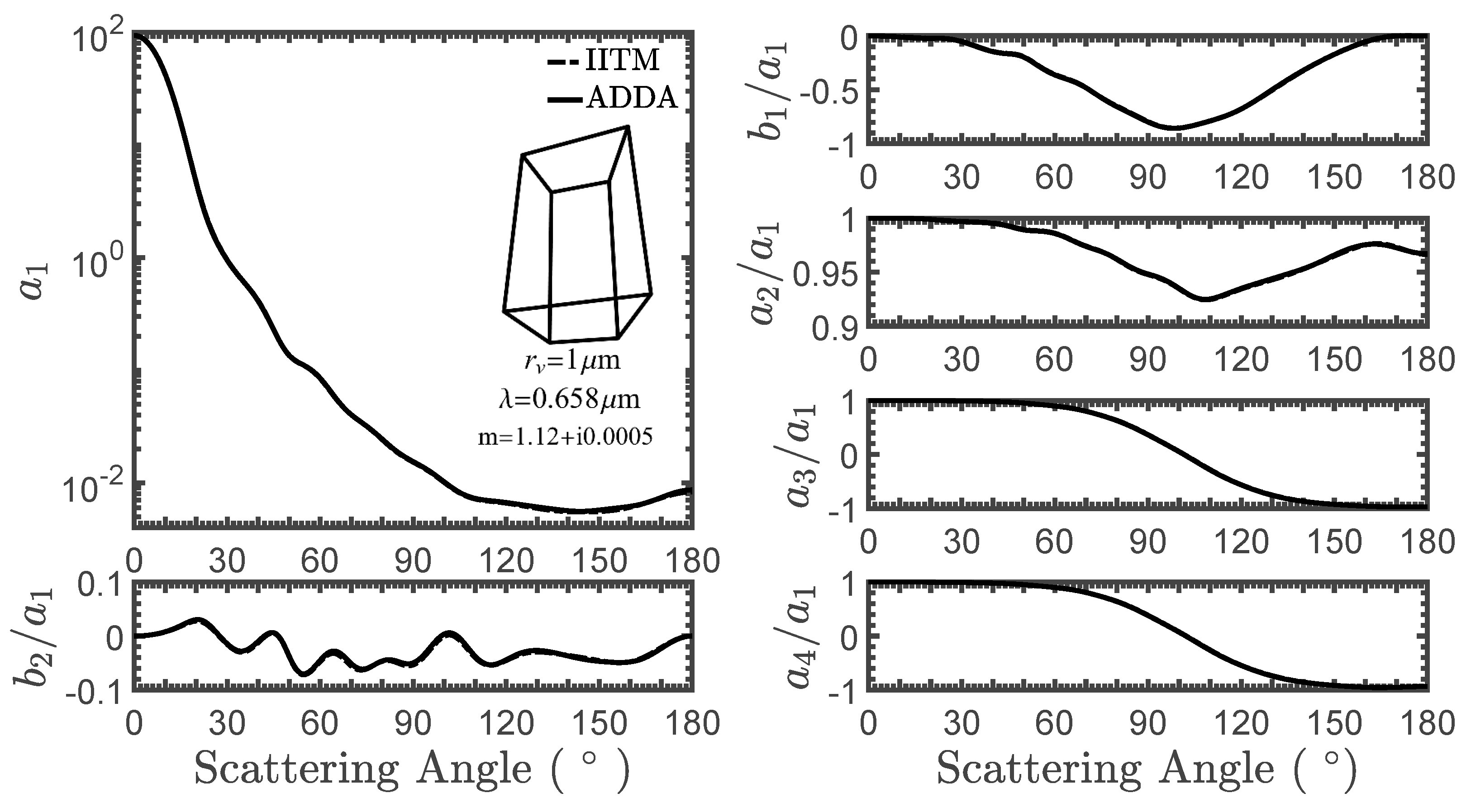
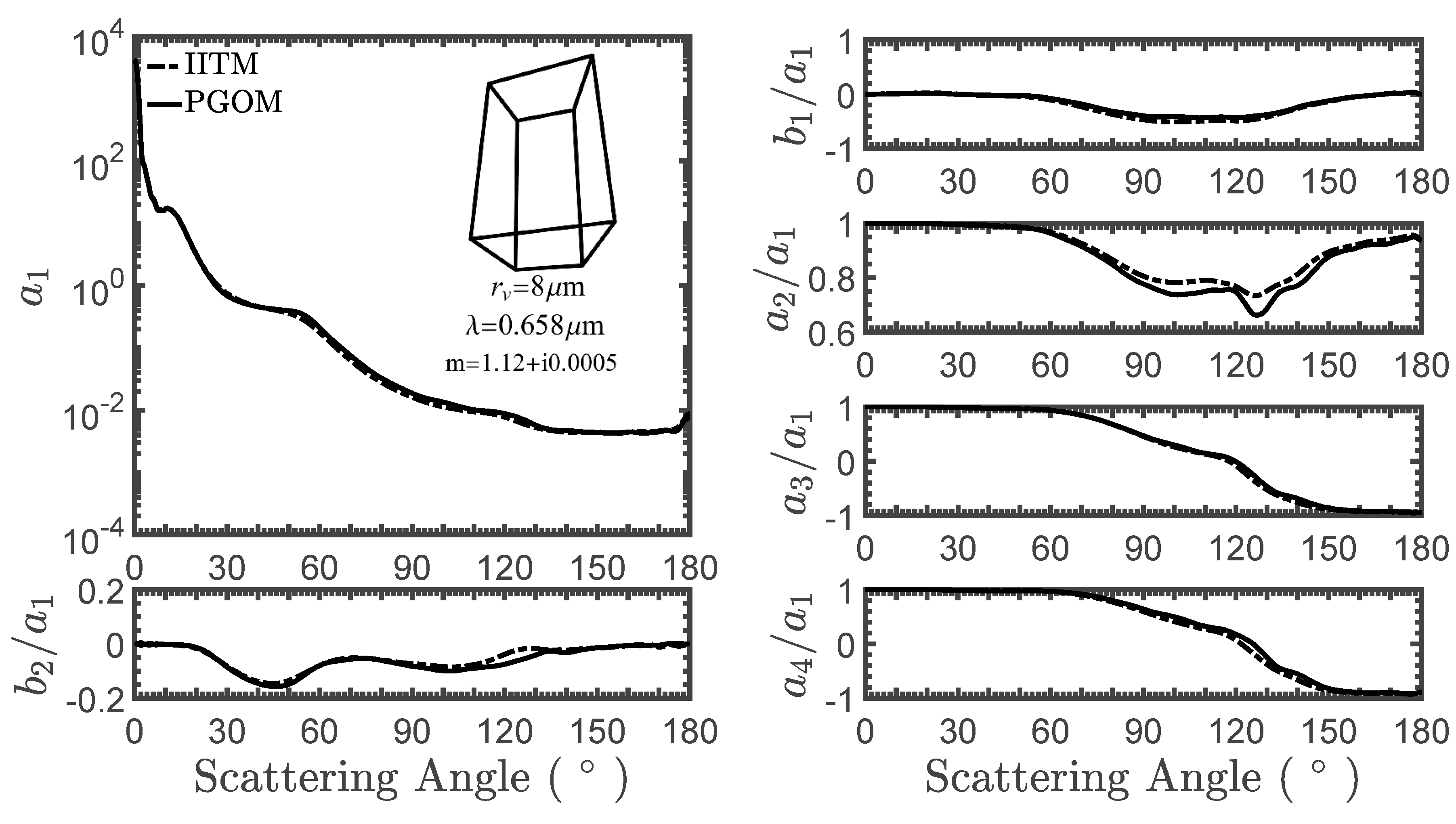
4.2. Oceanic Particle Simulation Using ADDA, IITM, and PGOM

Section 4.1 describes an example of dinoflagellates while using the ADDA to compute the 16 Mueller matrix elements that were given by Liu and Kattawar [43], where the chromosome of the dinoflagellate has complex helical structure and is simulated mostly in fixed orientations. Generally, a simple nonspherical shape in random orientation is used to simulate the optical properties of oceanic particles. A hexahedron particle here is used as an example of an oceanic particle to show how Mueller matrix elements can be calculated by three typical methods: the ADDA, the IITM, and the PGOM. The relative refractive index of the particle is set to be 1.12 + i0.0005 and the incident wavelength is 0.658 µm. Only the Mueller matrix of the particle under the random orientation condition is given.

Figure 3 shows the comparisons of the non-zero Mueller matrix elements calculated by the IITM and the ADDA. The volume equivalent radius is 1 µm. The element P₁₁ is normalized to give the normalized phase function while other elements are normalized by the element P₁₁. The simulation results calculated by the IITM and the ADDA are perfectly matched since they both are the exact solutions of Maxwell’s equations. However, the computation using the IITM is much more efficient than the computation using the ADDA since the random orientation process is realized by ADDA through considering a large number of orientations. On the other hand, the ADDA for a fixed orientation in this case is more efficient than the IITM since the IITM has to compute the T-matrix of the particle, regardless of whether it is in a fixed orientation or under the random orientation condition.

Figure 4 shows the comparisons of the Mueller matrix elements calculated by the IITM and the PGOM. The volume equivalent sphere radius is 8 µm. The PGOM results agree quite well with the IITM results, especially for the forward and backward scattering directions. Even though the PGOM is an approximate solution of Maxwell’s equation, the process of including the interference between the diffracted and transmitted rays and mapping the near field to the far field significantly enhances its accuracy. The advantage of the PGOM is that it is computationally much more efficient than the IITM.

5. Conclusions

A general introduction for calculating the Mueller matrix of suspended particles in the ocean is given. The surface and volume integral equations of the electromagnetic field can be given from Maxwell’s equations. Also, the amplitude scattering matrix and the Mueller matrix with respect to light scattering can be defined to describe the polarization state of a suspended particle. To calculate the amplitude scattering matrix and Mueller matrix, the scattering methods are introduced based on the following categories: numerically exact methods, semi-analytical T-matrix methods, and geometric optics methods. For clarity, three typical methods: the DDA method, the IITM, and the PGOM, are briefly presented. Moreover, the Mueller matrix of an arbitrarily generated hexahedron particle under the random orientation condition is computed while using the ADDA and the IITM when the volume equivalent sphere radius is 1 µm and using the PGOM and the IITM for a volume equivalent sphere with a radius of 8 µm, while the incident wavelength is 0.658 µm. Perfect agreement between the ADDA and the IITM are given since both methods are considered to be the exact solutions. The IITM is more computationally efficient than the ADDA when the particle is under the random orientation condition. Excellent agreement between the PGOM and the IITM are obtained especially for the forward and the backward scattering directions. The PGOM is more computationally efficient than the IITM because of the ray-tracing process. Consequently, the Mueller matrix of suspended particles can be computed by using numerically exact methods, T-matrix methods, and the physical-geometric optics method to cover a complete size range.

References

1. Stramski, D.; Kiefer, D.A. Light scattering by microorganisms in the open ocean. Prog. Oceanogr. 1991, 28, 343–383. [Google Scholar] [CrossRef]
2. Morel, A.; Bricaud, A. Theoretical results concerning the optics of phytoplankton, with special references to remote sensing applications. In Oceanography from Space; Gower, J.F.R., Ed.; Springer: Berlin, Germany, 1981; pp. 313–327. [Google Scholar]
3. Morel, A.; Bricaud, A. Inherent optical properties of algal cells, including picoplankton. Theorectical and experimental results. Can. Bull. Fish. Aquat. Sci. 1986, 214, 521–559. [Google Scholar]
4. Lerner, A.; Shashar, N.; Haspel, C. Sensitivity study on the effects of hydrosol size and composition on linear polarization in absorbing and nonabsorbing clear and semi-turbid waters. J. Opt. Soc. Am. A 2012, 29, 2394–2405. [Google Scholar] [CrossRef] [PubMed]
5. Tzabari, M.; Lerner, A.; Iluz, D.; Haspel, C. Sensitivity study on the effect of the optical and physical properties of coated spherical particles on linear polarization in clear to semi-turbid waters. Appl. Opt. 2018, 57, 5806–5822. [Google Scholar] [CrossRef] [PubMed]
6. Clavano, W.R.; Boss, E.; Karp-Boss, L. Inherent Optical Properties of Non-Spherical Marine-Like Particles—From Theory to Observation. In Oceanography and Marine Biology: An Annual Review; Gibson, R.N., Atkinson, R.J.A., Gordon, J.D.M., Eds.; Taylor & Francis: Didcot, UK, 2007; pp. 1–38. [Google Scholar]
7. Quinbyhunt, M.S.; Hunt, A.J.; Lofftus, K.; Shapiro, D.B. Polarized-light scattering studies of marine Chlorella. Limnol. Oceanogr. 1989, 34, 1587–1600. [Google Scholar] [CrossRef] [Green Version]
8. Meyer, R.A. Light scattering from biological cells: Dependence of backscattering radiation on membrane thickness and refractive index. Appl. Opt. 1979, 18, 585–588. [Google Scholar] [CrossRef] [PubMed]
9. Kitchen, J.C.; Zaneveld, J.R.V. A three-layered sphere model of the optical properties of phytoplankton. Limnol. Oceanogr. 1992, 37, 1680–1690. [Google Scholar] [CrossRef] [Green Version]
10. Quirantes, A.; Bernard, S. Light scattering by marine algae: Two-layer spherical and nonspherical models. J. Quant. Spectrosc. Radiat. Transf. 2004, 89, 311–321. [Google Scholar] [CrossRef]
11. Sun, B.; Kattawar, W.G.; Yang, P.; Twardowski, S.M.; Sullivan, M.J. Simulation of the scattering properties of a chain-forming triangular prism oceanic diatom. J. Quant. Spectrosc. Radiat. Transf. 2016, 178, 390–399. [Google Scholar] [CrossRef] [Green Version]
12. Mundy, W.C.; Roux, J.A.; Smith, A.M. Mie scattering by spheres in an absorbing medium. J. Opt. Soc. Am. 1974, 64, 1593–1597. [Google Scholar] [CrossRef]
13. Chylek, P. Light scattering by small particles in an absorbing medium. J. Opt. Soc. Am. 1977, 67, 561–563. [Google Scholar] [CrossRef]
14. Mishchenko, M.I.; Yang, P. Far-field Lorez-Mie scattering in an absorbing host medium: Theoretical formalism and FORTRAN program. J. Quant. Spectrosc. Radiat. Transf. 2018, 205, 241–252. [Google Scholar] [CrossRef]
15. Morse, P.M.; Feshbach, H. Methods of Theoretical Physics; McGraw-Hill: New York, NY, USA, 1953. [Google Scholar]
16. Bohren, C.F.; Huffman, D.R. Absorption and Scattering of Light by Small Particles; John Wiley & Sons: New York, NY, USA, 1983. [Google Scholar]
17. Parke, N.G., III. Optical Algebra. J. Math. Phys. 1949, 28, 131–139. [Google Scholar] [CrossRef]
18. Barakat, R. Bilinear constraints between elements of the 4 × 4 Mueller-Jones transfer matrix of polarization theory. Opt. Commun. 1981, 38, 159–161. [Google Scholar] [CrossRef]
19. Kattawar, G.W.; Yang, P.; You, Y.; Bi, L.; Xie, Y.; Huang, X.; Hioki, S. Polarization of light in the atmosphere and ocean. In Light Scattering Reviews 10: Light Scattering and Radiative Transfer; Kokhanovsky, A.A., Ed.; Springer: Berlin, Germany, 2016; pp. 3–39. [Google Scholar]
20. Van de Hulst, H.C. Light Scattering by Small Particles; John Wiley & Sons: New York, NY, USA, 1957. [Google Scholar]
21. Hu, C.; Kattawar, G.W.; Parkin, M.E.; Herb, P. Symmetry theorems on the forward and backward scattering Mueller matrices for light scattering from a nonspherical dielectric scatterer. Appl. Opt. 1987, 26, 4159–4173. [Google Scholar] [CrossRef] [PubMed]
22. Hovenier, J.W.; Mackowski, D.W. Symmetry relations for forward and backward scattering by randomly oriented particles. J. Quant. Spectrosc. Radiat. Transf. 1998, 60, 483–492. [Google Scholar] [CrossRef]
23. Mobley, C.D. Light and Water: Radiative Transfer in Natural Waters; Academic Press: San Diego, CA, USA, 1994. [Google Scholar]
24. Asano, S.; Yamamoto, G. Light scattering by a spheroidal particle. Appl. Opt. 1975, 14, 29–49. [Google Scholar] [CrossRef] [PubMed]
25. Asano, S.; Sato, M. Light scattering by randomly oriented spheroidal particles. Appl. Opt. 1980, 19, 962–974. [Google Scholar] [CrossRef] [PubMed]
26. Voss, K.J.; Fry, E.S. Measurement of the Mueller matrix for ocean water. Appl. Opt. 1984, 23, 4427–4439. [Google Scholar] [CrossRef] [PubMed]
27. Taflove, A.; Hagness, S.C. Computational Electrodynamics: The Finite-Difference Time-Domain Method; Artech House: Boston, MA, USA, 2000. [Google Scholar]
28. Yee, S.K. Numerical solution of initial boundary value problems involving Maxwell’s equations in isotropic media. IEEE Trans. Antennas Propag. 1966, 14, 302–307. [Google Scholar]
29. Yang, P.; Liou, K.N. Finite-difference time domain method for light scattering by small ice crystals in three-dimensional space. J. Opt. Soc. Am. A 1996, 13, 2072–2085. [Google Scholar] [CrossRef]
30. Yang, P.; Liou, K.N. Finite difference time domain method for light scattering by nonspherical and inhomogeneous particles. In Light Scattering by Nonspherical Particles; Mishchenko, M.I., Hovenier, J.W., Travis, L.D., Eds.; Academic Press: San Diego, CA, USA, 2000; pp. 173–221. [Google Scholar]
31. Berenger, J.P. A perfectly matched layer for the absorption of electromagnetic waves. J. Comput. Phys. 1994, 114, 185–200. [Google Scholar] [CrossRef]
32. Silvester, P.P.; Ferrari, R.L. Finite Elements for Electrical Engineers; Cambridge University Press: Cambridge, UK, 1996. [Google Scholar]
33. Morgan, M.; Mei, K. Finite-element computation of scattering by inhomogeneous penetrable bodies of revolution. IEEE Trans. Antennas Propag. 1979, 27, 202–214. [Google Scholar] [CrossRef]
34. Press, W.H.; Flannery, B.P.; Teukolsky, S.A.; Vetterling, W.T. Numerical Recipes; Cambridge University Press: Cambridge, UK, 1989. [Google Scholar]
35. Purcell, E.M.; Pennypacker, C.R. Scattering and absorption of light by nonspherical dielectric grains. Astrophys. J. 1973, 186, 705–714. [Google Scholar] [CrossRef]
36. Draine, B.T. The discrete-dipole approximation and its application to interstellar graphite grains. Astrophys. J. 1988, 333, 848–872. [Google Scholar] [CrossRef]
37. Draine, B.T. The Discrete Dipole Approximation for Light Scattering by Irregular Targets; Academic Press: San Diego, CA, USA, 2000; pp. 131–144. [Google Scholar]
38. Yurkin, M.A.; Hoekstra, A.G. The discrete-dipole-approximation code ADDA: Capabilities and known limitations. J. Quant. Spectrosc. Radiat. Transf. 2011, 112, 2234–2247. [Google Scholar] [CrossRef]
39. Draine, B.T.; Flatau, P.J. User guide for the discrete dipole approximation code DDSCAT 7.3. arXiv, 2013; arXiv:1305.6497. [Google Scholar]
40. Yurkin, M.A.; Hoekstra, A.G. User Manual for the Discrete Dipole Approximation Code ADDA 1.3b4. 2014. Available online: http://a-dda.googlecode.com/svn/tags/rel_1.3b4/doc/manual.pdf (accessed on 6 May 2018).
41. Gordon, R.H.; Smyth, J.T.; Balch, M.W.; Boynton, C.G.; Tarran, A.G. Light scattering by coccoliths detached from Emiliania huxleyi. Appl. Opt. 2009, 48, 6059–6073. [Google Scholar] [CrossRef] [PubMed]
42. Zhai, P.W.; Hu, Y.; Trepte, C.R.; Winker, D.M.; Josset, D.B.; Lucker, P.L.; Kattawar, G.W. Inherent optical properties of the coccolithophore: Emiliania huxleyi. Opt. Express 2013, 21, 17625–17638. [Google Scholar] [CrossRef] [PubMed]
43. Liu, J.; Kattawar, G.W. Detection of dinoflagellates by the light scattering properties of the chiral structure of their chromosomes. J. Quant. Spectrosc. Radiat. Transf. 2013, 131, 24–33. [Google Scholar] [CrossRef]
44. Waterman, P.C. Matrix formulation of electromagnetic scattering. Proc. IEEE 1965, 53, 805–812. [Google Scholar] [CrossRef]
45. Waterman, P.C. Symmetry, unitarity, and geometry in electromagnetic scattering. Phys. Rev. D 1971, 3, 825. [Google Scholar] [CrossRef]
46. Tsang, L.; Kong, J.A.; Ding, K.H. Scattering of electromagnetic waves. In Theories and Applications; Wiley: Hoboken, NJ, USA, 2000; Volume 1. [Google Scholar]
47. Mishchenko, M.I.; Travis, L.D.; Mackowski, D.W. T-matrix computations of light scattering by nonspherical particles: A review. J. Quant. Spectrosc. Radiat. Transf. 1996, 55, 535–575. [Google Scholar] [CrossRef]
48. Mishchenko, M.I.; Travis, L.D.; Lacis, A.A. Scattering, Absorption, and Emission of Light by Small Particles; Cambridge University Press: Cambridge, UK, 2002. [Google Scholar]
49. Mishchenko, M.I.; Travis, L.D. Capabilities and limitations of a current FORTRAN implementation of the T-matrix method for randomly oriented, rotationally symmetric scatterers. J. Quant. Spectrosc. Radiat. Transf. 1998, 60, 309–324. [Google Scholar] [CrossRef]
50. Doicu, A.; Wriedt, T.; Eremin, Y.A. Light Scattering by Systems of Particles: Null-Field Method with Discrete Sources: Theory and Programs; Springer: Berlin, Germany, 2006; Volume 124. [Google Scholar]
51. Johnson, B.R. Invariant imbedding T matrix approach to electromagnetic scattering. Appl. Opt. 1988, 27, 4861–4873. [Google Scholar] [CrossRef] [PubMed]
52. Bi, L.; Yang, P.; Kattawar, G.W.; Mishchenko, M.I. Efficient implementation of the invariant imbedding T-matrix method and the separation of variables method applied to large nonspherical inhomogeneous particles. J. Quant. Spectrosc. Radiat. Transf. 2013, 116, 169–183. [Google Scholar] [CrossRef]
53. Bi, L.; Yang, P. Accurate simulation of the optical properties of atmospheric ice crystals with the invariant imbedding T-matrix method. J. Quant. Spectrosc. Radiat. Transf. 2014, 138, 17–35. [Google Scholar] [CrossRef]
54. Bi, L.; Yang, P. Impact of calcification state on the inherent optical properties of Emiliania huxleyi coccoliths and coccolithophores. J. Quant. Spectrosc. Radiat. Transf. 2015, 155, 10–21. [Google Scholar] [CrossRef]
55. Born, M.; Wolf, E. Principles of Optics; Cambridge University Press: Cambridge, UK, 1999. [Google Scholar]
56. Takano, Y.; Liou, K.N. Solar radiative transfer in cirrus clouds. Part I: Single-scattering and optical properties of hexagonal ice crystals. J. Atmos. Sci. 1989, 46, 3–19. [Google Scholar] [CrossRef]
57. Macke, A.; Mueller, J.; Raschke, E. Single scattering properties of atmospheric ice crystals. J. Atmos. Sci. 1996, 53, 2813–2825. [Google Scholar] [CrossRef]
58. Yang, P.; Liou, K.N. Geometric-optics—Integral-equation method for light scattering by nonspherical ice crystals. Appl. Opt. 1996, 35, 6568–6584. [Google Scholar] [CrossRef] [PubMed]
59. Muinonen, K. Scattering of light by crystals: A modified Kirchhoff approximation. Appl. Opt. 1989, 28, 3044–3050. [Google Scholar] [CrossRef] [PubMed]
60. Yang, P.; Liou, K.N. Light scattering by hexagonal ice crystals: Solutions by a ray-by-ray integration algorithm. JOSA A 1997, 14, 2278–2289. [Google Scholar] [CrossRef]
61. Bi, L.; Yang, P.; Kattawar, G.W.; Hu, Y.; Baum, B.A. Scattering and absorption of light by ice particles: Solution by a new physical-geometric optics hybrid method. J. Quant. Spectrosc. Radiat. Transf. 2011, 112, 1492–1508. [Google Scholar] [CrossRef]
62. Borovoi, A.G.; Grishin, I.A. Scattering matrices for large ice crystal particles. JOSA A 2003, 20, 2071–2080. [Google Scholar] [CrossRef] [PubMed]
63. Sun, B.; Yang, P.; Kattawar, G.W.; Zhang, X. Physical-geometric optics method for large size faceted particles. Opt. Express 2017, 25, 24044–24060. [Google Scholar] [CrossRef] [PubMed]
64. Nayak, A.R.; Mcfarland, M.N.; Sullivan, J.M.; Twardowski, M.S. Evidence for ubiquitous preferential particle orientation in representative oceanic shear flows. Limnol. Oceanogr. 2018, 63, 122–143. [Google Scholar] [CrossRef] [PubMed]
65. Heil, C.A.; Steidinger, K.A. Monitoring, management, and mitigation of Karenia blooms in the eastern Gulf of Mexico. Harmful Algae 2009, 8, 611–617. [Google Scholar] [CrossRef]
66. Kiefer, D.A.; Olson, R.J.; Wilson, W.H. Reflectance spectroscopy of marine phytoplankton. part I. optical properties as related to age and growth rate. Limnol. Oceanogr. 1979, 24, 664–672. [Google Scholar] [CrossRef]
67. Steidinger, K.A.; Truby, E.W.; Dawes, C.J. Ultrastructure of the red tide dinoflagellate Gymnodinium breve. I. General description 2.3. J. Phycol. 1978, 14, 72–79. [Google Scholar] [CrossRef]
68. Rizzo, P.J.; Jones, M.; Ray, S.M. Isolation and properties of isolated nuclei from the Florida red tide dinoflagellate Gymnodinium breve (Davis). J. Protozool. 1982, 29, 217–222. [Google Scholar] [CrossRef] [PubMed]
69. Gautier, A.; Michel-Salamin, L.; Tosi-Couture, E.; McDowall, A.W.; Dubochet, J. Electron microscopy of the chromosomes of dinoflagellates in situ: Confirmation of Bouligand’s liquid crystal hypothesis. J. Ultrastruct. Mol. Struct. Res. 1986, 97, 10–30. [Google Scholar] [CrossRef]
70. Rill, R.L.; Livolant, F.; Aldrich, H.C.; Davidson, M.W. Electron microscopy of liquid crystalline DNA: Direct evidence for cholesteric-like organization of DNA in dinoflagellate chromosomes. Chromosoma 1989, 98, 280–286. [Google Scholar] [CrossRef] [PubMed]
71. Shapiro, D.B.; Quinbyhunt, M.S.; Hunt, A.J. Origin of the Induced circular-polarization in the light-scattering from a dinoflagellate. Ocean Opt. X 1990, 1302, 281–289. [Google Scholar]
72. Shapiro, D.B.; Hunt, A.J.; Quinby-Hunt, M.S.; Hull, P.G. Circular-polarization effects in the light-scattering from single and suspensions of dinoflagellates. Underw. Imaging Photogr. Visibility 1991, 1537, 30–41. [Google Scholar]
73. Bouligand, Y.; Soyer, M.O.; Puiseux-Dao, S. La structure fibrillaire et l’orientation des chromosomes chez les Dinoflagellés. Chromosoma 1968, 24, 251–287. [Google Scholar] [CrossRef] [PubMed]
Figure 1. Parameters used for light scattering by a dielectric particle. The field point r is outside the scattering particle with wavenumber k, permittivity ε , and permeability μ 0 and the point r ' is inside the particle with wave number k1, permittivity ε 1 , and permeability μ 0 .
Applsci 08 02686 g001
Figure 2. Discretization of a particle volume in the discrete-dipole approximation (DDA) method.
Applsci 08 02686 g002
Figure 3. Comparisons of Mueller matrix elements of a hexahedron particle calculated by the invariant-imbedding T-matrix method (IITM) and the ADDA. The volume equivalent sphere radius is 1µm and the incident wavelength is 0.658 µm. The relative refractive index is 1.12 + i0.0005.
Applsci 08 02686 g003
Figure 4. Comparisons of Mueller matrix elements of a hexahedron particle calculated by the IITM and the physical-geometric optics method (PGOM). The volume equivalent sphere radius is 8 µm and the incident wavelength is 0.658 µm. The relative refractive index is 1.12 + i0.0005.
Applsci 08 02686 g004