Article

Uncertainty Evaluation for Measurements of Pitch Deviation and Out-of-Flatness of Planar Scale Gratings by a Fizeau Interferometer in Littrow Configuration

1
Precision Nanometrology Laboratory, Department of Finemechanics, Tohoku University, Sendai 980-8579, Japan
2
State Key Laboratory for Digital Manufacturing Equipment and Technology, Huazhong University of Science and Technology, Wuhan 430074, China
*
Author to whom correspondence should be addressed.
Appl. Sci. 2018, 8(12), 2539; https://doi.org/10.3390/app8122539
Submission received: 25 October 2018 / Revised: 27 November 2018 / Accepted: 5 December 2018 / Published: 7 December 2018
(This article belongs to the Special Issue Precision Dimensional Measurements)

Abstract

:
Form errors of a planar scale grating, such as pitch deviations and out-of-flatness, are major contributors to the final measurement uncertainty of an interferential scanning-type planar encoder. Following the previous work, in which a method has been proposed to evaluate both the out-of-flatness and the pitch deviations of a planar scale grating by a Fizeau interferometer in Littrow configuration, uncertainty analysis on this method is performed in this paper. Theoretical equations are derived to make quantitative uncertainty analysis while taking possible error factors into account. To overcome the drawbacks of a traditional uncertainty matrix approach, a new procedure is proposed to evaluate the uncertainty in the PV (peak-to-valley) deviation of a surface form, so as to assure the quality of measurement. Experiments are finally conducted to demonstrate the feasibility of proposed uncertainty evaluation method.

1. Introduction

An optical encoder, which is mainly composed of an optical sensor head and a scale grating, is one of the most commonly used sensors for precision positioning in production engineering [1], due to the advantages of non-contact measurement, a high resolution, and a wide bandwidth [2]. In the case of incremental type one-axis encoders, a diffraction grating having periodic line pattern structures is employed as a scale for measurement of relative translational displacement between the scale grating and an optical sensor head [3]. With the employment of a planar scale grating having two-dimensional grating pattern structures [4], the dimension of displacement/position measurement can be expanded to two or more [5,6]. Among the components in a multi-axis planar encoder system [5], a planar scale grating having periodical structures along the X- and Y-directions is one of the key components that influence the accuracy of measurement, since the period of interference signal in the optical head, which will be interpolated and used to calculate the displacement, is directly influenced by the pitch of the scale grating, in principle [4]. Moreover, the Z-directional out-of-flatness of the scale grating could also be a source of measurement uncertainty in the planar encoder system. The X- and Y-directional pitch deviations, as well as the out-of-flatness of the scale grating, are thus required to be evaluated and calibrated over the entire surface of a scale grating for high precision measurement applications [7].
Line scale comparator [8,9] and scanning probe microscopes (SPMs) [10,11] are available as conventional solutions to evaluate the pitch deviations of a planar scale granting. The line scale comparator has long been used in the enterprises that manufacture linear encoders and national standard institutes for testing one-axis linear scale gratings [8,9]. However, it is too expensive to construct a measurement system for two-dimensional scale grating that is based on the line scale comparator. Another drawback of the line scale comparator is that the out-of-flatness of a planar scale grating cannot be measured in principle. Meanwhile, SPMs can measure both the grating pitch deviations and the out-of-flatness of a planar scale grating. However, on the other hand, a limited scanning area and a measurement throughput of SPMs [11] prevent them being applied for the evaluation of planar scale grating, especially for the condition of laboratory-level, it may take hours and days to conduct the measurement of a large size planar scale grating over its whole area.
In responding to the background described above, the authors’ group has proposed a method to simultaneously evaluate both the X- and Y-directional pitch deviations and the Z-directional out-of-flatness of a planar scale grating by utilizing a Fizeau interferometer in the previous work [7]. In the propose method, wavefront of the zeroth-order diffracted beam and wavefronts of positive and negative first-order diffracted beams from a scale grating obtained in Littrow configurations were utilized to perform a non-contact evaluation of a planar scale grating over the entire area. The feasibility of proposed method has been verified in experiments [7]. In addition, the proposed method has been improved so that the self-calibration of the Fizeau interferometer and the planar scale grating can be conducted simultaneously while considering the out-of-flatness of the reference optical flat and the change of the coordinate system in the Littrow configuration [12]. As the first step of the research, a preliminary verification of the improved method has been performed successfully through the simulation in both the noise-free and noisy cases [12]. The key advantage of this method is that the measurement using the Fizeau interferometer can be carried out without significant investments in time and/or capital to assess the out-of-flatness and pitch deviations of the planar scale grating accurately compared with other measurement techniques. Nevertheless, further experimental demonstration as well as the uncertainty analysis of the proposed method have not been conducted yet, and they remain to be addressed.
In this paper, as the second step of the research, experimental verification of the feasibility of the improved method [12] has been conducted as well as the uncertainty analysis when considering the possible error factors influencing the measurement uncertainties, such as the form error of the reference surface in a Fizeau interferometer or the inclination error of a scale grating in measurement. Theoretical equations are derived to evaluate the influence of the error factors on the final uncertainties in the measured Z-directional out-of-flatness as well as the X- and Y-directional pitch deviations of a scale grating. Moreover, when considering the drawbacks of the traditional uncertainty matrix approach [13], which is intellectually satisfying but difficult to handle or specify the surface form in a straightforward way, a method aiming to evaluate the uncertainty by using one of the simplest but most commonly used peak-to-valley (P-V) deviation of the surface form is proposed. Experiments are also conducted to demonstrate the feasibility of the proposed method.

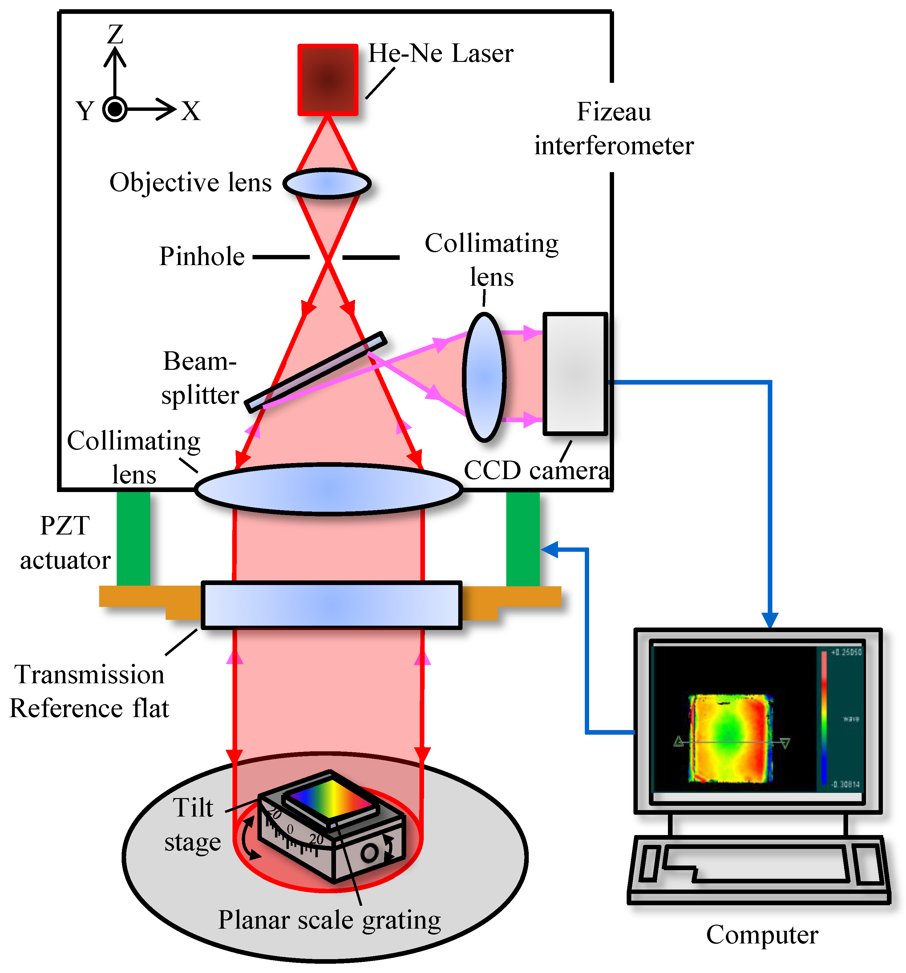
2. Measurement Principle

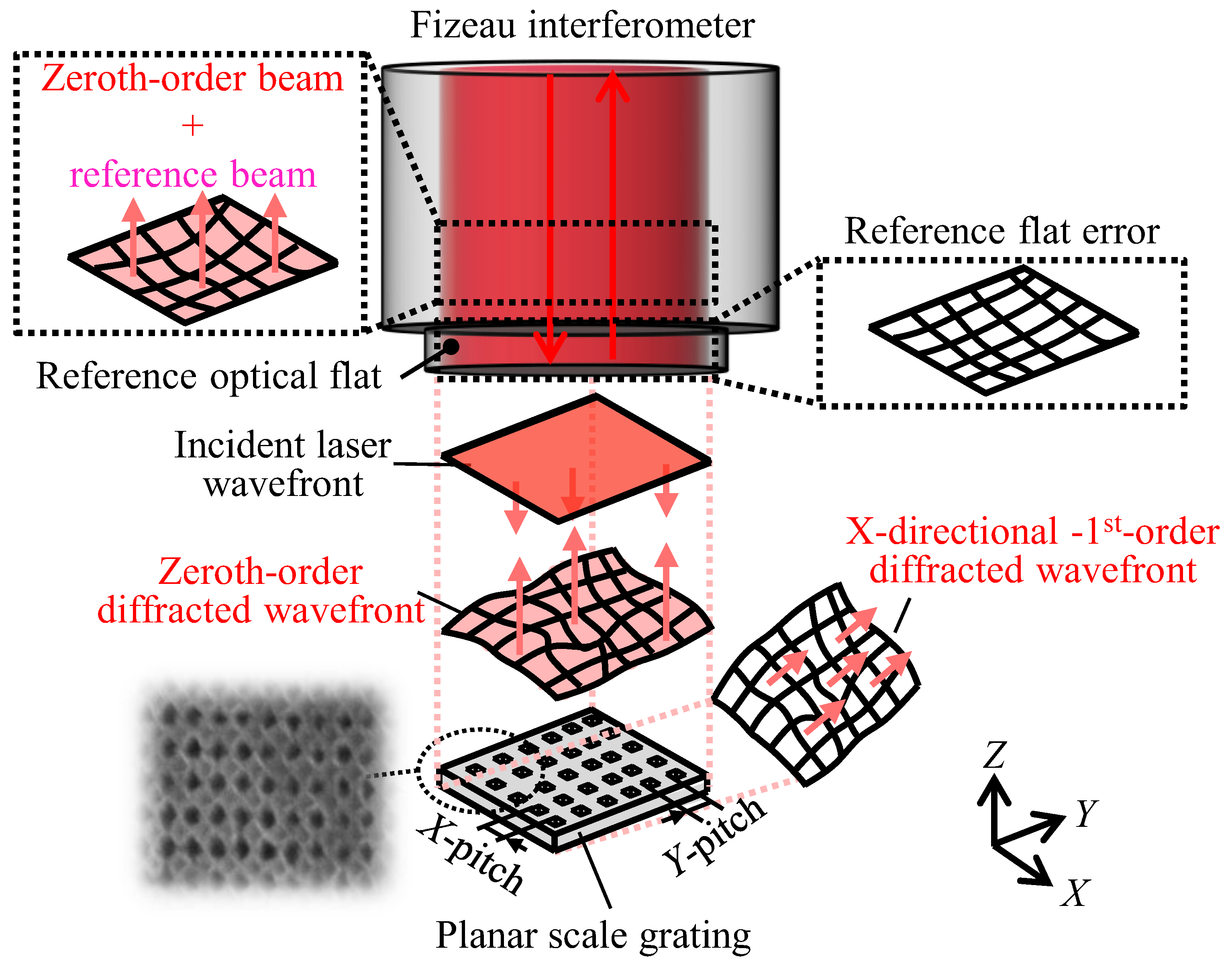
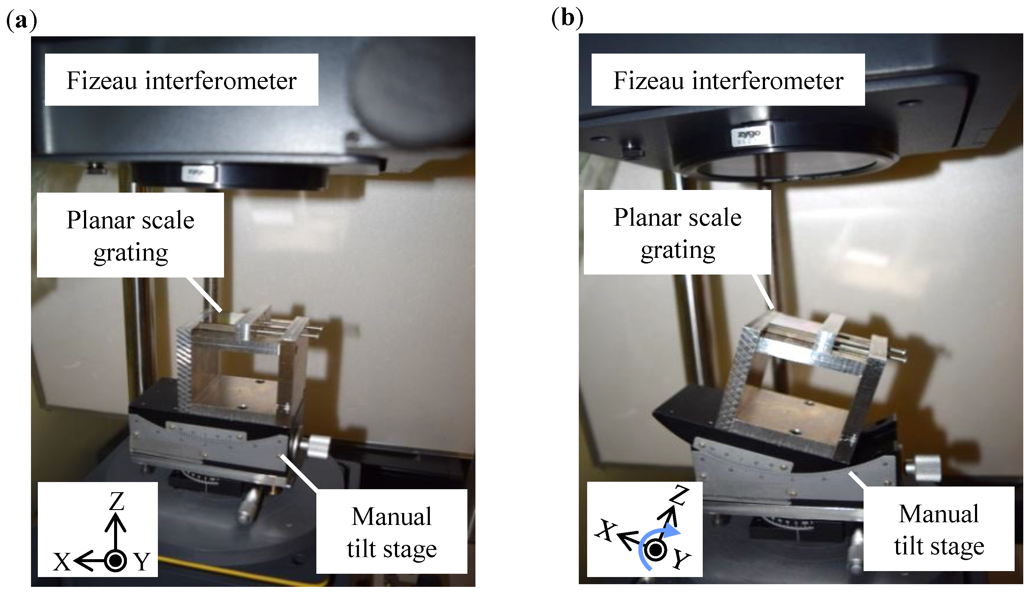
Figure 1 demonstrates the measurement of the Z-directional out-of-flatness of a planar scale grating eZ(x,y) using the typical function of the Fizeau interferomter. Assume that the field-of-view (FOV) of the Fizeau interferometer is larger than the size of the grating employed for measurement. As can be seen in the figure, the wavefront of the zeroth-order diffracted beam from the grating superimposed on the wavefront of the reflected beam from the reference optical flat. Consequently, the zeroth-order phase output I0(x,y) from the interferometer can be expressed by the following equation [7]:
I 0 ( x , y ) = 4 π [ e Z ( x , y ) e R ( x , y ) ] λ
where λ represents the light wavelength of the laser source and eR(x,y) represents the out-of-flatness of the reference optical flat in the Fizeau interferometer. The out-of-flatness of the grating eZ(x,y) can be obtained by the following equation according to Equation (1):
e Z ( x , y ) = λ 4 π I 0 ( x , y ) + e R ( x , y )
As can be seen in Equation (2), the result of eZ(x,y) contains the out-of-flatness of the reference flat eR(x,y). Since the calibration of the absolute flatness of the reference flat is quite complicated in practice [14], in this paper, the mean (average or expectation) of eR(x,y) is taken to be zero and its uncertainty being the specified peak-to-valley (PV) value, which is typically less than λ/20 over the whole field of view (FOV) of a commercial Fizeau interferometer.
For the evaluation of X-directional pitch deviation eX(x,y) and Y- directional pitch deviation eY(x,y) of the planar scale grating, measurement of the wavefronts of the X and Y-directional positive and negative first-order diffracted beams in Littrow configurations is needed. 
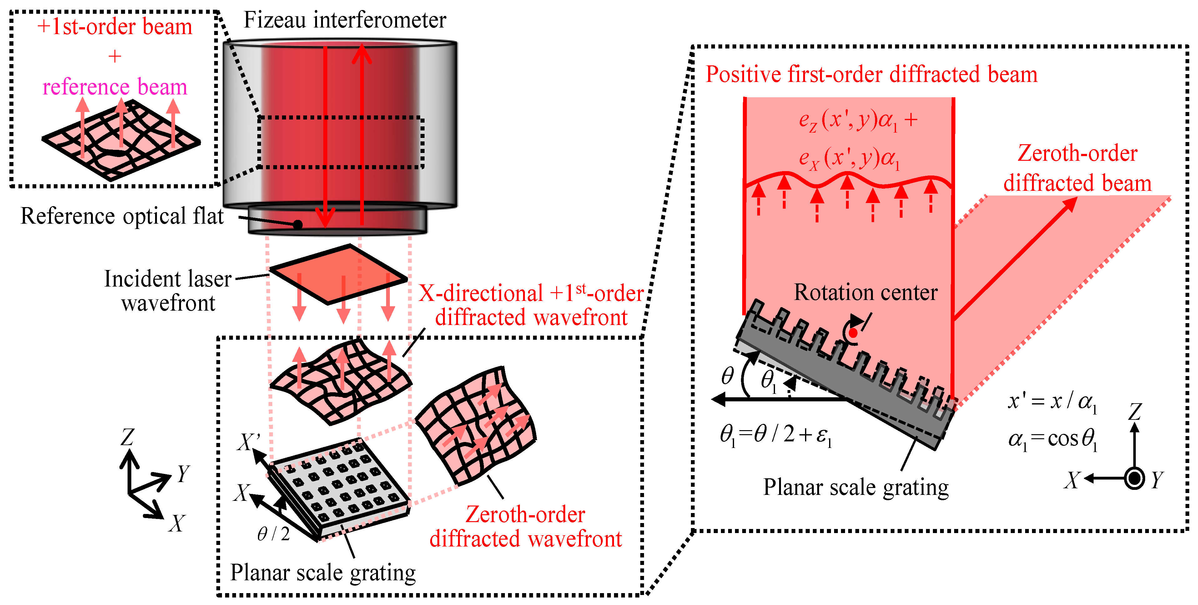
Figure 2 shows an example of the Littrow configuration for the measurement of the wavefront of X-directional positive first-order diffracted beam, where the grating is tilted clockwise, so that the X-directional positive first-order diffracted beam is back-reflected directly into the direction of the incident laser beam and superimposed with the reference beam in the Fizeau interferometer. Assume that the actual inclination angle in measurement θ1 can be represented by θ1 = θ/2 + ε1, where θ = arcsin(λ/g) is the first-order diffraction angle, ε1 is the misalignment of θ, and g is the nominal pitch of the grating along the X-direction. The X-directional pitch deviation eX(x,y) of the planar scale grating causes a phase shift in the wavefront of the diffracted beam [7]. As depicted in Figure 2, the coordinate system has changed after setting the grating in Littrow configuration. Since the measurement results should correspond to the original grating coordinate system, the X-directional positive first-order phase output IX+1(x,y) that was obtained in the Fizeau measurement can be described, as follows:
I X + 1 ( x , y ) = 2 π e X ( x / α 1 , y ) g + 4 π λ [ α 1 e Z ( x / α 1 , y ) e R ( x , y ) ]
where α1 = cosθ1. In the same manner, the wavefront of the X-directional negative first-order diffracted beam can be measured by tilting the scale grating counterclockwise with an opposite inclination angle, the X-directional negative first-order phase output IX−1(x,y) can be obtained, as follows:
I X 1 ( x , y ) = 2 π e X ( x / α 2 , y ) g + 4 π λ [ α 2 e Z ( x / α 2 , y ) e R ( x , y ) ]
where α2 = cosθ2. By using the error ε2 in the alignment of θ2 in measurement of the negative first-order diffracted beam, θ2 can be represented as θ2 = −θ/2 + ε2. According to Equations (3) and (4), the following equation can be obtained:
e X ( x / α 1 , y ) + e X ( x / α 2 , y ) = g 2 π [ I X + 1 ( x , y ) I X 1 ( x , y ) ] 2 g λ [ α 1 e Z ( x / α 1 , y ) α 2 e Z ( x / α 2 , y ) ]
In the same manner, the Y-directional pitch deviation eY(x,y) of the planar scale grating can be obtained as follows by measuring the Y-directional positive and negative first-order phase outputs IY+1(x,y) and IY−1(x,y), respectively:
I Y + 1 ( x , y ) = 2 π e Y ( x , y / α 1 ) g + 4 π λ [ α 1 e Z ( x , y / α 1 ) e R ( x , y ) ] ,
I Y 1 ( x , y ) = 2 π e Y ( x , y / α 2 ) g + 4 π λ [ α 2 e Z ( x , y / α 2 ) e R ( x , y ) ] ,
where α 1 = cosθ1 = cos(θ/2 + ε1) and α2 = cosθ2 = cos(θ/2 + ε2). ε1 and ε2 represent the misalignments of θ in the measurement of the wavefronts of the Y-directional positive and negative first-order diffracted beams, respectively. Note here that the nominal pitches of the planar scale grating along the X- and Y-directions are assumed to be the same for the sake of simplicity. According to Equations (6) and (7), the following equation can be obtained:
e Y ( x , y / α 1 ) + e Y ( x , y / α 2 ) = g 2 π [ I Y + 1 ( x , y ) I Y 1 ( x , y ) ] 2 g λ [ α 1 e Z ( x , y / α 1 ) α 2 e Z ( x , y / α 2 ) ]
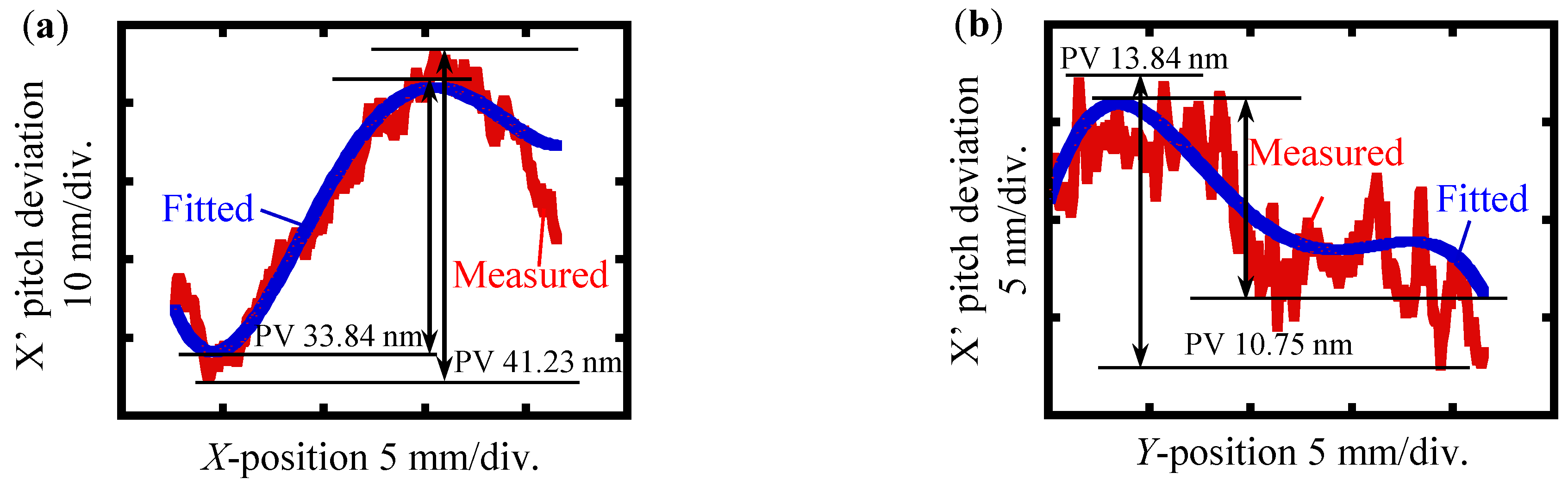
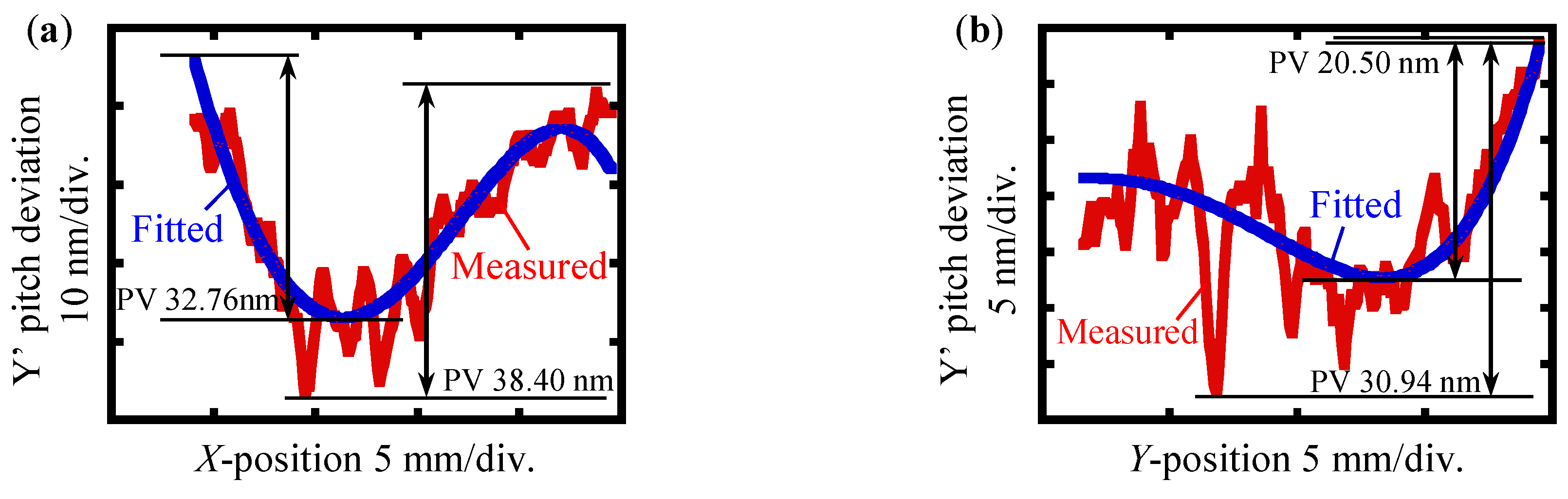
In the following section of this paper, how to further obtain the mean values and uncertainties of eZ(x,y), eX(x,y), and eY(x,y) according to Equations (2), (5), and (8) are presented. Since the evaluations of the mean value and uncertainty of eY(x,y) are similar to those of eX(x,y), only the latter is focused in the following for the sake of clarity.

3. Uncertainty Evaluation

Major sources of uncertainty in the evaluation of out-of-flatness eZ(x,y) and pitch deviation eX(x,y) of a planar scale grating by a Fizeau interferometer primarily arise from uncertainties in the measured phase outputs I0(x,y) and IX±1(x,y). In addition, out-of-flatness eR(x,y) of the reference flat in a Fizeau interferometer and uncertainties in the nominal pitch g of the planar scale grating under test, as well as the inclination angles θ1 and θ2, could also be major sources of uncertainty. According to the GUM (guide to the expression of uncertainty in measurement) [13], the uncertainties in I0(x,y) and IX±1(x,y) attribute to the Type A evaluation, while those in eR(x,y), g, θ1 and θ2 attribute to the Type B evaluation. Through the uncertainty analysis, The E(·), σ(·) and σ2(·) are used to represent the mean, standard deviation, and variance of a random variable, respectively. The expanded uncertainty of a random variable is given by u(·) = (·), where k denotes the coverage factor; k = 2 produces a confidence interval of approximately 95%; and, k = 3 produces an interval with a confidence of approximately 99%.
As mentioned in Section 2, in this paper, the mean and 3σ uncertainty of eR(x,y) are treated to be zero and the specified PV value, respectively. The uncertainty in the inclination angles θ1 and θ2 contains two components; one is the uncertainty induced by the deviation of the nominal grating pitch with respect to its true value, and another is induced by the misalignments in measurement. In the uncertainty analysis, the means of θ1 and θ2 are taken to be θ/2 and −θ/2, respectively, and the uncertainties that are induced by the misalignments are assumed to be identical; namely, σ(ε1) = σ(ε2). Due to the independence between θ and ε1 (ε2), the means of α1 and α2 will be cos(θ/2), which is denoted as α in the following (α = cos(θ/2)). By taking the means for both sides of Equations (2) and (5), the following equations can be obtained:
E [ e Z ( x , y ) ] = λ 4 π E [ I 0 ( x , y ) ] ,
E [ e X ( x / α , y ) ] = g 4 π { E [ I X + 1 ( x , y ) ] E [ I X 1 ( x , y ) ] } ,
It should be pointed out that here has E[α1eZ(x/α1,y)] = E[α2eZ(x/α2,y)] mathematically. In practical experiments, the second term of the right side of Equation (5) could be minimized by making interference fringes of the Fizeau interferometer minimum though adjusting the tilt stage on which the scale grating is fixed. Although the influence from the out-of-flatness of the substrate surface cannot completely be eliminated by the differential operation, when considering the holographic grating with a good surface quality, the effect on the evaluation of the pitch deviation can be ignored by conducting the operation mentioned above.
A straightforward approach to evaluate the uncertainty in the obtained eZ(x,y) and eX(x,y) is to generate a matrix, called the uncertainty matrix [15], which has the same size to eZ(x,y) or eX(x,y) and it contains the corresponding uncertainty of eZ(x,y) or eX(x,y) at every pixel position (xi,yj) (I = 1, 2, …, M; j = 1, 2, …, N). Taking the propagation of errors into consideration, the variances σ2[eZ(x,y)] and σ2[eX(x/α,y)] can be represented, as follows:
σ 2 [ e Z ( x , y ) ] = ( λ 4 π ) 2 σ 2 [ I 0 ( x , y ) ] + σ 2 [ e R ( x , y ) ] ,
σ 2 [ e X ( x / α , y ) ] = ( g 4 π ) 2 { σ 2 [ I X + 1 ( x , y ) ] + σ 2 [ I X 1 ( x , y ) ] } + { E [ e X ( x / α , y ) ] g } 2 σ 2 ( g ) + 2 [ g λ e Z ( x / α , y ) + g λ α e Z ( x / α , y ) α ] 2 σ 2 ( α ) + 2 ( g λ α ) 2 σ 2 [ e Z ( x / α , y ) ] ,
where the variance σ2(α) is evaluated by the following equation:
σ 2 ( α ) = sin 2 ( θ 2 ) { [ 1 2 1 1 ( λ / g ) 2 λ g 2 ] 2 σ 2 ( g ) + σ 2 ( ε ) } .
The first and second terms in curly brackets of the right side of Equation (13) correspond to the uncertainties that are induced by the deviation of the nominal grating pitch to its true value and the misalignment in measurement, respectively. It should be noted from Equations (11) and (12) that, for eZ(x,y), the corresponding uncertainty matrix can be obtained, while for eX(x,y) it cannot, because of the change in the coordinate system after tilting the scale gating. Moreover, as shown in Equation (12), even for eX(x/α,y), the corresponding uncertainty matrix cannot be obtained either due to the involvement of the evaluation of the unknown eZ(x/α,y), ∂eZ(x/α,y)/∂α, and σ2[eZ(x/α,y)]. On the other hand, it should be pointed out that the uncertainty matrix approach has a number of drawbacks in practice. As stated in [16], the information density that is contained in the uncertainty matrix is too high for users who only want a single number. In addition, the uncertainty matrix cannot easily be used for the decision of either acceptance or rejection. Evaluations of measurement uncertainty should be expressed in a manner that is informative and actionable [17]. Therefore, in this paper, a PV value is adopted to evaluate the quality of the obtained form errors. Although a PV value also has inadequacies in charactering surfaces, it is still widely recognized that a PV value remains one of the most commonly used specifications of surface form errors [18]. Next, the details are presented in evaluating a PV value and its uncertainty for the characterization of eZ(x,y) and eX(x,y).
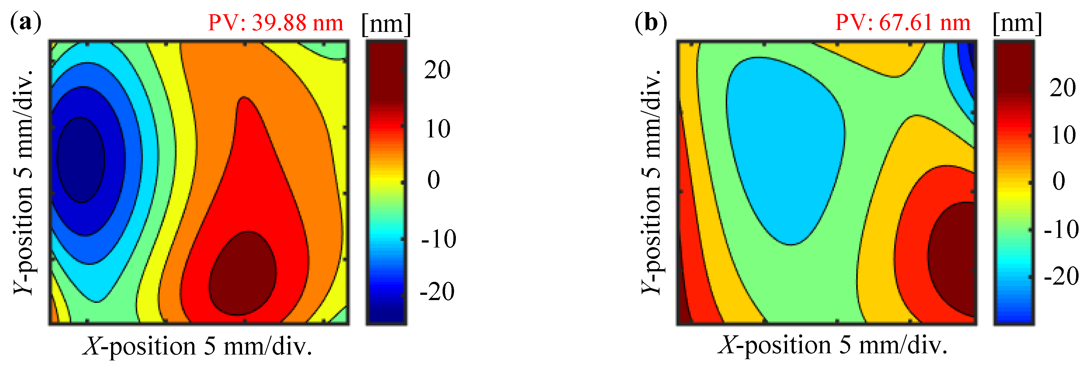
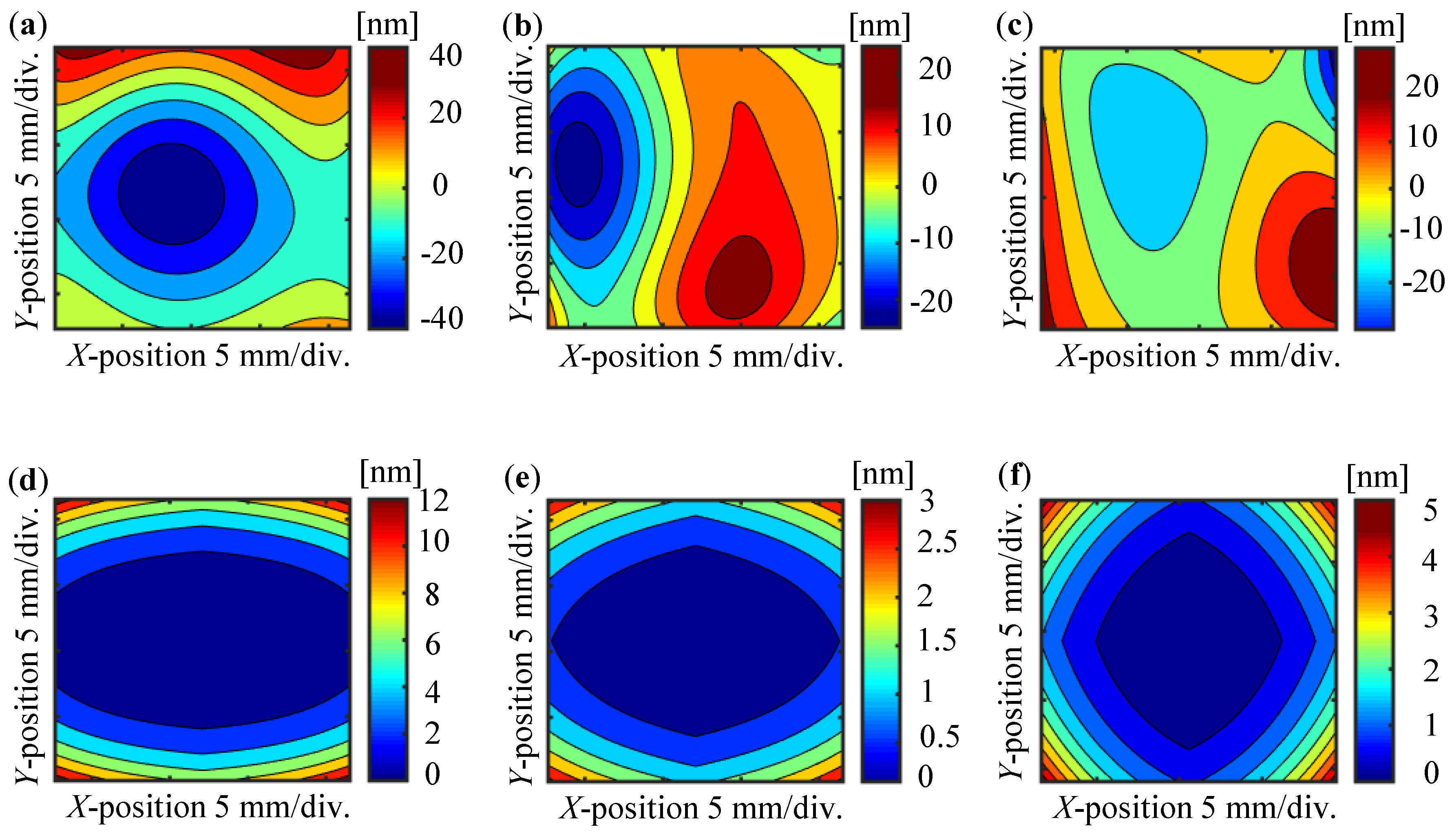
In this paper, the form errors eZ(x,y) and eX(x,y) are assumed can be characterized in terms of polynomials. This assumption is reasonable, since, as stated in [19], the low-frequency errors can be completely modeled by the set of polynomials and are of the main concern in the application. Moreover, modeling the form errors in terms of polynomials is also favorable to evaluate the associated PV values since the estimated PV values will not be biased by the high-frequency noises contained in the raw data. Without losing generality, the n-degree bivariate polynomials are used to fit the discrete form errors (xi, yj, E[eZ(xi,yj)]) and (xi, yj, E[eX(xi/α,yj)]) obtained at each pixel position (xi,yj), according to Equations (9) and (10), as follows:
e Z ( x , y ) = [ 1 , x , x 2 , , x n ] [ A 00 A 01 A 02 A 0 , n A 10 A 11 A 1 , n 1 A 20 A 2 , n 2 A n 0 0 ] [ 1 y y 2 y n ] = x T A y ,
e X ( x / α , y ) = [ 1 , x , x 2 , , x n ] [ B 00 B 01 B 02 B 0 , n B 10 B 11 B 1 , n 1 B 20 B 2 , n 2 B n 0 0 ] [ 1 y y 2 y n ] = x T B y ,
where the matrices A and B′ contain the undetermined coefficients of the fitted bivariate polynomials. As noted from Equations (14) and (15), here the set of n-degree bivariate polynomials are used to fit the form errors of the scale grating. In addition, the highest degree for x and y coordinates is not necessary to be identical, but it depends on the actual fitting performance. With Equations (14) and (15), the eZ(x/α,y) and eX(x,y) can be obtained, as follows:
e Z ( x / α , y ) = x T A y ,
e X ( x , y ) = x T B y ,
where
A = [ 1 1 / α 1 / α 2 1 / α n ] [ A 00 A 01 A 02 A 0 , n A 10 A 11 A 1 , n 1 A 20 A 2 , n 2 A n 0 0 ] ,
B = [ 1 α α 2 α n ] [ B 00 B 01 B 02 B 0 , n B 10 B 11 B 1 , n 1 B 20 B 2 , n 2 B n 0 0 ]
According to Equations (14), (16), and (18), once the matrix A is obtained, the eZ(x/α,y), ∂eZ(x/α,y)/∂α, σ2[eZ(x/α,y)] can also be calculated successively, and finally σ2[eX(x/α,y)] by Equation (12), eZ(x/α,y) by Equation (16), eX(x,y) by Equations (17) and (19), and also σ2[eX(x,y)]. With the obtained eZ(x,y), σ2[eZ(x,y)], eX(x,y), and σ2[eX(x,y)], evaluation of the PV values and the associated uncertainty for both eZ(x,y) and eX(x,y) can also be conducted. Since the procedures for obtaining the matrices A and B′ are similar, only the determination of the matrix A is presented in the following.
Taking the vectorization operator on both sides of Equation (14) leads to
vec [ e Z ( x , y ) ] = ( y T x T ) vec ( A ) ,
where vec(·) signifies the vectorization operator that converts a matrix into a column vector, and the symbol represents the Kronecker product. Discarding the zero elements in vec(A) and denoting the processed vec(A) as a vector a = [a0, a1, a2, …, aK−1]T (K = (n + 1)(n + 2)/2) and then choosing new basis functions Ξk (k = 0, 1, 2, …, K−1), where Ξk {1, x, y, x2, xy, y2, …, xyn−1, yn}, the Equation (20) can be rewritten, as follows:
η ( ξ ) = a 0 Ξ 0 ( ξ ) + a 1 Ξ 1 ( ξ ) + a 2 Ξ 2 ( ξ ) + + a K 1 Ξ K 1 ( ξ ) ,
where the variable ξ represents the value of the terms x, y, x2, xy, y2, …, xyn−1, yn at any pixel position (xi,yj) (i = 1, 2, …, M; j = 1, 2, …, N), and η(ξ) represents the value of vec[eZ(x,y)] at the corresponding pixel position. To determine the elements in vector a, the general linear least-squares method [20] is used by defining a merit function, as follows:
χ 2 = l = 1 M N [ η l k = 0 K 1 a k Ξ k ( ξ l ) σ ( η l ) ] 2 ,
where ηl corresponds to the value E[eZ(xi,yj)] given in Equation (9) and σ(ηl) is corresponding standard deviation σ[eZ(xi,yj)], as obtained by Equation (11). In addition, an MN × K matrix D, which is also called the design matrix of the fitting problem, is defined with elements given as follows:
D l k = Ξ k ( ξ l ) σ ( η l ) .
Also, define a vector b of length MN with elements, as follows:
b l = η l σ ( η l ) .
The minimum of Equation (22) occurs where the derivative of χ2 with respect to all K parameters ak vanish. This condition yields the following matrix equation:
( D T D ) a = D T b .
According to Equation (25), the least-squares estimation of vector a can be obtained, as follows:
a ^ = ( D T D ) 1 D T b = D + b ,
where D+ = (DTD)−1DT is the Moore-Penrose pseudo-inverse of D. Let’s denote the matrix (DTD)−1 as C, namely, C = (DTD)−1, which is also called the covariance matrix and it has a close relation with the uncertainties of the estimated parameters ak (k = 0, 1, 2, …, K − 1) by Equation (26). Specifically, the variance in ak can be evaluated by
σ 2 ( a ^ k ) = C k k ,
where Ckk is the k-th diagonal element of the matrix C. According to Equations (26) and (27), the least-square estimation Apq (p,q = 0, 1, 2, …, n) of all elements in matrix A as well as their uncertainties u(Apq) can be finally obtained.
With the estimated elements Apq and their uncertainties u(Apq), the uncertainty of eZ(x,y) at any pixel position (xi,yj) can be further evaluated. Specifically, according to Equation (14), there is eZ(xi,yj) = xiTAyj, which can be regarded as a linear function of the coefficients Apq. The evaluation of the upper and lower bounds of eZ(xi,yj) can be transformed into a simple linear programming problem [21], described as follows:
{ max e Z ( x i , y j ) = x i T A y j s . t . A p q [ A ^ p q u ( A ^ p q ) , A ^ p q + u ( A ^ p q ) ]     p , q = 0 , 1 , 2 , , n ,
{ min e Z ( x i , y j ) = x i T A y j s . t . A p q [ A ^ p q u ( A ^ p q ) , A ^ p q + u ( A ^ p q ) ]     p , q = 0 , 1 , 2 , , n ,
where Equations (28a) and (28b) yield the upper and lower bounds of eZ(xi,yj), respectively. The uncertainty of eZ(x,y) at the pixel position of (xi,yj) is then evaluated by
u [ e Z ( x i , y j ) ] = e Z ¯ ( x i , y j ) e Z _ ( x i , y j ) 2 .
In addition, according to Equation (18), the least-squares estimation Apq of elements in matrix A′ can be calculated, as follows:
A ^ p q = 1 α p A ^ p q .
It follows that the uncertainty in Apq can be evaluated by the following equation:
u 2 ( A ^ p q ) = ( p α p + 1 A ^ p q ) 2 u 2 ( α ) + ( 1 α p ) 2 u 2 ( A ^ p q ) .
With Apq and u(Apq), the values of eZ(x/α,y) and ∂eZ(x/α,y)/∂α can be obtained at any pixel position of (xi,yj). The uncertainty of eZ(x/α,y) at any pixel position (xi,yj) can be also evaluated in a similar manner to Equation (28). Likewise, the value of eX(x,y) and its uncertainty u[eX(x,y)] at any pixel position (xi,yj) can be calculated as well.
The PV value of eZ(x,y) in the region Ω of interest can be evaluated by
PV [ e Z ( x , y ) ] = max [ e Z ( x , y ) ] min [ e Z ( x , y ) ] , ( x , y ) Ω ,
where max(·) and min(·) represent the maximum and minimum of a function. The peak and valley values of eZ(x,y), max[eZ(x,y)], and min[eZ(x,y)] can be readily calculated according to the obtained expression of eZ(x,y). The uncertainty in the calculated PV of eZ(x,y) can then be evaluated, as follows:
u 2 { PV [ e Z ( x , y ) ] } = u p 2 [ e Z ( x , y ) ] + u v 2 [ e Z ( x , y ) ] ,
where up[eZ(x,y)] and uv[eZ(x,y)] represent the uncertainties of eZ(x,y) at the peak and valley positions, respectively, which can be directly obtained by substituting the coordinates of the peak and valley positions into Equation (29).
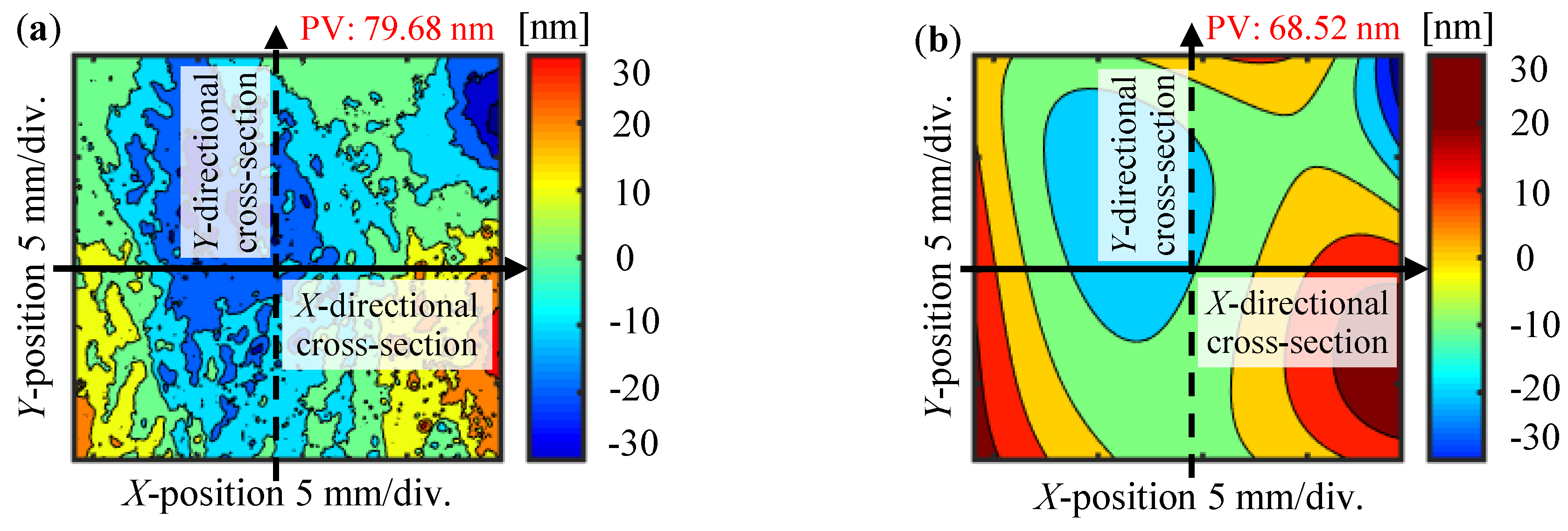
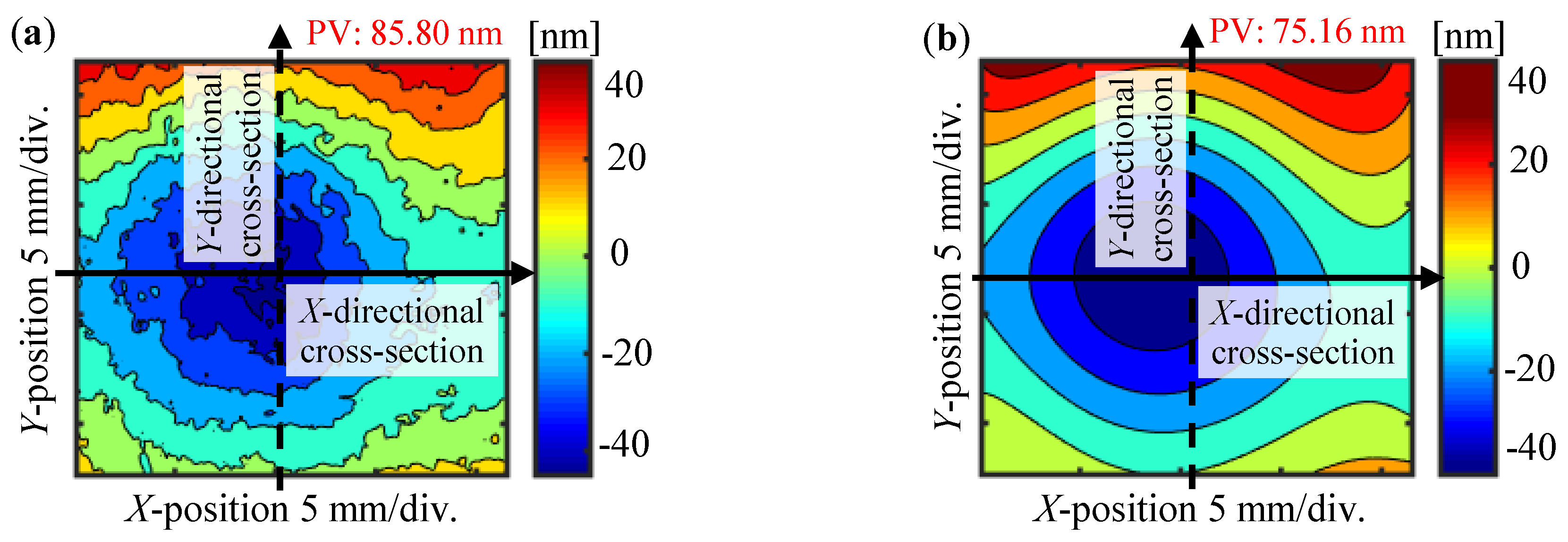
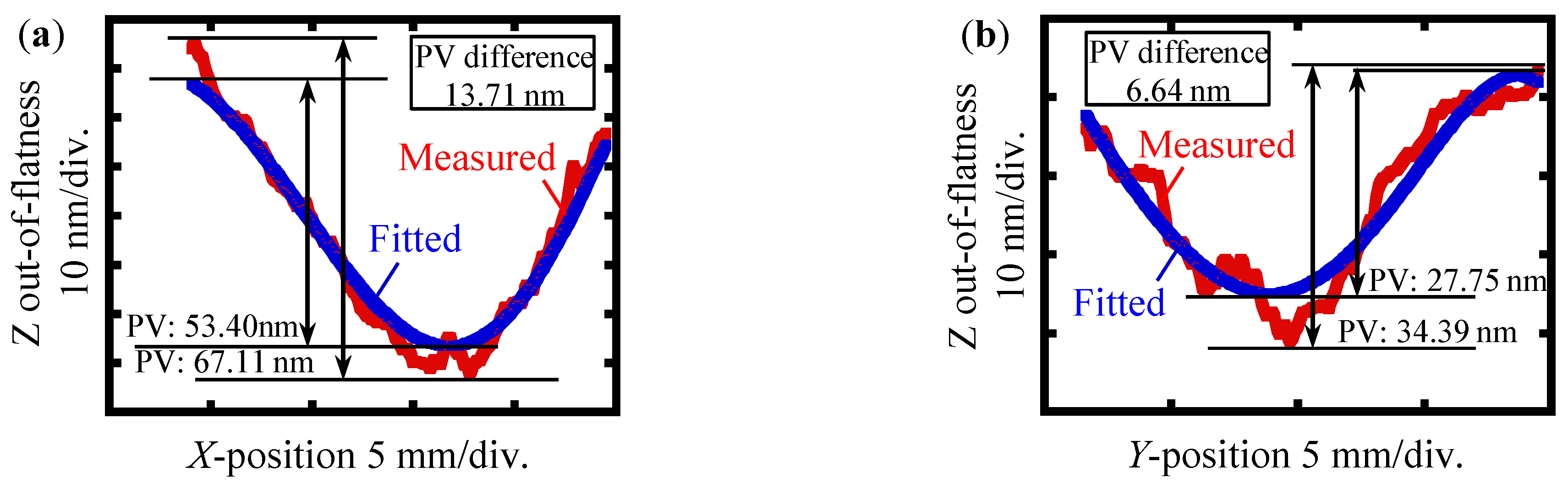
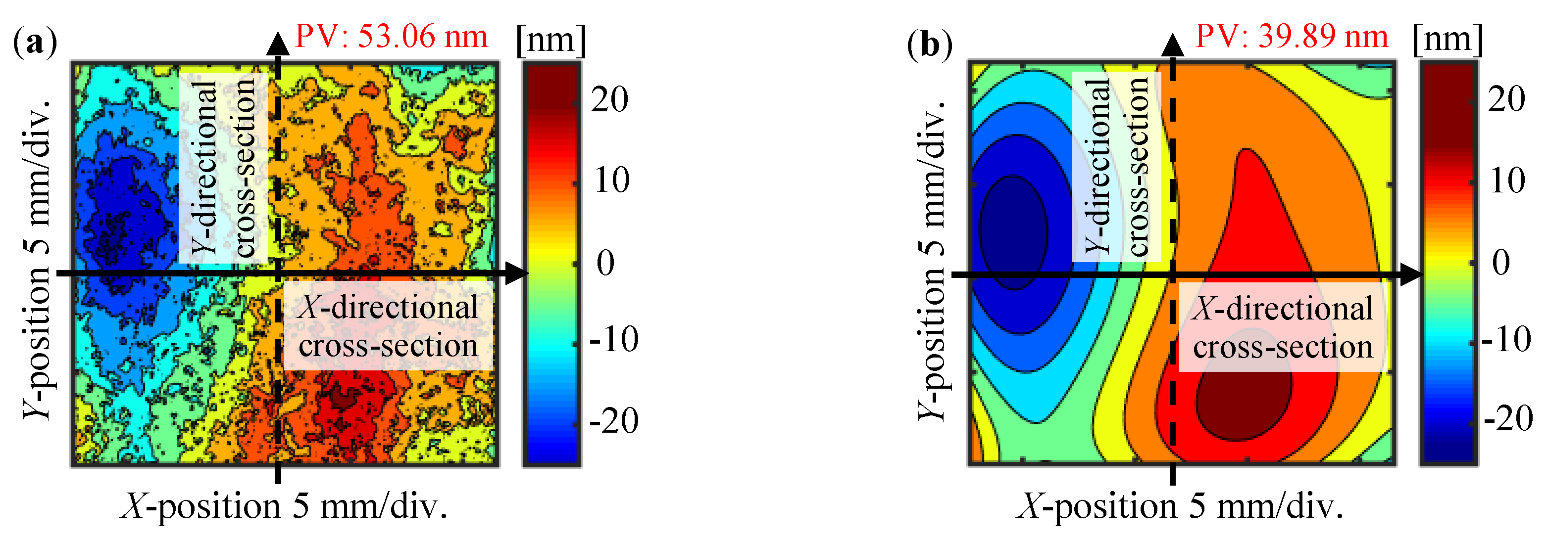
Other approaches to evaluate the uncertainty in PV could simply double the maximum value of the uncertainty matrix or applying the Monte Carlo (MC) simulation. However, the former method obviously overestimates the uncertainty in the PV, except coincidence. The MC method could estimate the PV uncertainty by collecting the PV value in each trail assuming that all of the significant errors are included and the probability distributions of each error source is known. Nevertheless, it is burdensome to run the simulation when routine experiment is conducted in a similar condition and the noise could exist explicitly in the evaluated results. Therefore, in this paper, the MC method is not employed, but just the part of error form is analyzed directly to evaluate the uncertainty in the peak and valley separately, and then combine them together. Since the PV of each error form is usually larger than the uncertainty in this experiment, this method is thus a reasonable way to obtain the uncertainty in PV.
As can be noted from the above description, the success of the proposed evaluation method lies on the fitting performance of the polynomials fitted to eZ(x,y) and eX(x/α,y). There are two measures that are commonly used to evaluate the goodness-of-fit in statistics. One is the coefficient of determination R2, while another is the reduced chi-square χ2, which for the polynomial fitted to eZ(x,y) are defined, as follows:
R 2 = 1 l = 1 M N [ η l k = 0 K 1 a ^ k Ξ k ( ξ l ) ] l = 1 M N [ η l l = 1 M N η l / M N ] ,
χ v 2 = χ min 2 v = 1 M N K l = 1 M N [ η l k = 0 K 1 a ^ k Ξ k ( ξ l ) σ ( η l ) ] 2 ,
where v = MN × K signifies the degree-of-freedom in the least-square regression. Typically, 0 < R2 < 1, and the larger the R2 is, the better the polynomial model fits the data. For the reduced chi-square, χv2 = 1 indicates that the model properly fits the data, while χ v 2 > 1 indicates that the fit does not fully capture the data (or that the variance σ2(ηl) is underestimated) and χ v 2 < 1 indicates that the model overly fits the data (either the model improperly fits the noise or the variance σ2(ηl) is overestimated). According to the value of χ v 2 , the variance of ak that is represented in Equation (27) is usually rescaled as follows in order to pass the χ2-test:
σ r 2 ( a ^ k ) = χ v 2 C k k ,
In addition, as illustrated in Equation (26), the least-squares estimation of vector a can be obtained by calculating the Moore-Penrose pseudo-inverse of the design matrix D. It should be pointed out that this solving approach is susceptible to round-off error in practice and it will lead to errors in both the solution a and its uncertainty, especially when the variance σ2(ηl) (corresponds to the variance σ2(eZ(xi,yj))) is not uniform at different pixel positions. To relieve the round-off problem, the solution by use of the singular value decomposition is recommended [22].

4. Experiments

4.1. Experimental Setup

A commercial Fizeau interferometer (VerifireTM, Zygo Corp, Middlefield, CT, USA) having a laser source with a wavelength of 632.8 nm was used in experiments. A field-of-view (FOV) of the Fizeau interferometer was 100 mm in diameter. Vertical and horizontal resolutions of the interferometer were 0.05 nm and 300 μm, respectively. A nominal PV value of the reference optical flat in the interferometer was less than λ/20 over the whole FOV. Figure 3 shows the experimental setup with the Fizeau interferometer. In the experiments, a reflective-type planar scale grating in a size of 35 mm × 30 mm that was fabricated by interference lithography was tested. This holographic planar scale grating had a nominal grating pitch of 1 μm along the X- and Y-directions. The scale grating was first mounted on a manual tilt stage and then together mounted on the sample stage in the Fizeau interferometer. Phase shifts in the wavefronts of diffracted beams caused by the out-of-flatness and pitch deviations of the scale grating can directly be measured by the Fizeau interferometer by setting the scale grating in the Littrow configuration. Although measuring higher-order diffracted beams would be helpful to enhance the measurement sensitivity, it requires a lager rotation angle, resulting in degradations of the quality of measured wavefront and the lateral resolution along the direction perpendicular to the grating grooves. Therefore, only the first-order diffracted beams were measured in the following experiments.
The zeroth-order diffracted wavefront was firstly measured to evaluate the out-of-flatness of the planar scale grating. After that, the scale grating was rotated clockwise and counterclockwise about the Y-axis by using the manual tilt stage to measure the X-directional positive and negative first-order diffracted beams, respectively. The inclination angle of the planar scale grating was adjusted by the manual tilt stage. With the visual feedback of the fringe pattern from the monitor in the Fizeau interferometer system, the number of interference fringes can be made to be minimum while adjusting the tilt stage. In the same manner, the Y-directional positive and negative first-order diffracted beams were also measured by rotating the tilt stage 90 degrees about the Z-axis. Figure 4a,b show photographs of the setup for measurement of the zeroth-order diffracted beam and the X-directional positive and negative first-order diffracted beams, respectively. Totally, it spent about 10 min to complete the experiments procedure, including the adjustment of the tilt stage and the alignment process of the Fizeau interferometer to minimize the number of fringes. Once the positive and negative first-order diffracted beams in both the X- and Y-directions are measured, the uncertainty evaluation can be conducted based on the models that are proposed in the previous section.

4.2. Results and Discussions

The form errors of the tested grating were first fitted by the set of n-degree bivariate polynomials, as proposed in Section 3. The highest degree n of the x and y coordinates in the respective model was set to be identical, which was 5 for the fitting of the Z-directional out-of-flatness error map and was 4 for the fitting of the X and Y-directional pitch deviations error maps for the sake of clarity. The regression surface may be too sharp or wiggly in the higher degree case. In addition, the higher degree polynomials will have problems with numerical accuracy. Therefore, the highest degree of the n-degree bivariate polynomials for each fitting model was selected not to exceed 5. Before the least square approximation, the x and y coordinates were normalized by the Z-score method [23] for a better fitting performance. In addition, the calculated variances from Equations (11) and (12) were used as the weights in the weighted least squared fitting process for fitting the corresponding error forms to make the approximation more precise. The fitting performance characterized by the proposed criterion in Section 3 was summarized in Table 1. As can be seen in the table, the values of R2 and χν of each model indicate that the set of polynomials well captured the error forms in the three directions. The small root-mean-square error (RMSE) values also show that the regression surface closely fits the measured form errors without the loss of precision. In the following, the comprehensive comparisons of the calibration results and polynomials fitting results of each directional form error are obtained.
An area of 20 mm × 20 mm over the scale grating located near the center of FOV was extracted for the evaluations. Figure 5a shows the out-of-flatness of the planar scale grating that was obtained in the experiment. The PV value was evaluated to be 85.80 nm. Figure 5b shows the polynomials fitting result of the measured out-of-flatness, as shown in Figure 5a. The PV value was evaluated to be 75.16 nm. To take a closer look at the fitting detail, the central cross-sections of the two results were extracted and compared with each other. Figure 6a,b show the X- and Y-directional central cross-sections of the out-of-flatness shown in Figure 5. The differences in the PV values between the measured result and the fitted results of the X- and Y-directional cross-sections were evaluated to be 13.71 nm and 6.64 nm, respectively. The X′-directional pitch deviation was also evaluated. Figure 7 shows the measured X′-directional deviation (eX(x′,y)) obtained by analyzing the phase outputs of the positive and negative fist-order diffracted beams that were measured by the commercial Fizeau interferometer. Figure 8 shows the X- and Y-directional central cross-sections of the pitch deviation that are shown in Figure 7. The PV of the X’-directional pitch deviation from the measured and fitted results were evaluated to be 53.06 nm and 39.89 nm, respectively.
In the same manner, the Y′-directional deviation (eY(x,y′)) was also evaluated as shown in Figure 9. The PV of the Y′-directional pitch deviation from the measured and fitted results were evaluated to be 79.68 nm and 68.52 nm, respectively, as shown in Figure 9. It should be noted that the PV values of the central XY axes cross-sections from the X′- and Y′-directional deviations were almost within 10 nm, as shown in Figure 8 and Figure 10; when considering the existence of the high frequency components in the original measurement data, the actual fitting error may be even smaller. Therefore, the fitted results could express the measured forms well with the existence of noise even though the PV value was small, which is acceptable for the precision requirement of the proposed evaluation methods.
The error maps of the X- and Y- directional pitch deviations were finally obtained based on the fitted results of eX(x′,y) and eY(x,y′), as shown in Figure 11a,b. The PV values of the fitted X- and Y-directional pitch deviations were evaluated to be 39.88 nm and 67.61 nm, respectively. It should be noted that the differences of the PV values in the fitted pitch deviation errors between the original X-, Y-directional results shown in Figure 11 and the tilted X′-,Y′-directional results shown in Figure 7b and Figure 9b were evaluated to be 0.01 nm and 0.91 nm, respectively, which were negligibly small, since the required Littrow angle was small and the newly calculated regression coefficients were similar to the original coefficients according to Equation (30). In addition, the analyzed area has slightly shifted after changing the coordinate system in the Littrow configuration back to the original grating coordinate system. It could be readily explained by the cosine impact from the inclination angle, which would induce a shift of the analyzed area with a distance determined by the cosine value of the inclination angle. However, since the influence of the inclination angle is already considered in the regression coefficients calculation of the polynomial fitting and the uncertainty evaluation process for the new area according to Equations (30) and (31), the finally obtained PV values and the PV uncertainties will thus not be overestimated after changing the coordinate system.
Table 2 shows the uncertainty budget. Since the complete model is quite complex, only the major uncertainty sources were taken into consideration, as discussed in Section 3. During the period of experiment, the environment effects, such as the air pressure, relative humidity, and temperature, could induce a drift in air refractive index as well as the laser wavelength. However, the refractive index drift and laser wavelength fluctuation in the whole measurement can be small under a well-controlled experimental environment with a limited testing time, which could be roughly estimated to be several picometers [24] and the caused combined errors are negligibly small. Therefore, the environmental effects and laser wavelength fluctuation are not problems in this experiment and its uncertainty is omitted in Equation (12). In addition, the angular displacement errors of the scale grating about the X- and Y-axes during the experiment were small, thus the misalignment angles due to the rotation error with respect to the X-and Y-axes do not contribute significantly to the overall combined uncertainty. Moreover, since this paper has focused on the form errors and PV uncertainties evaluation of the planar scale grating, the rotational error about the Z-axis is not a problem either in this case; the phase shifts information in the diffracted wavefronts will not change and the rotation error about the Z-axis is believed to be very small with careful adjustments.
Since the tested location of the planar scale grating was near the center of the FOV of the Fizeau interferometer, the PV value of the reference optical flat was expected to be far better than λ/20 in the experiment. In the uncertainty analysis, the standard uncertainty of the out-of-flatness of the reference optical flat is thereby taken to be σ[eR(x,y)] = λ/300, according to the size of the analyzed region of the grating under test. The standard uncertainty of the grating pitch was taken as u(g) = 100 nm, which was obtained by the specification sheet of the grating provided by the grating manufacturer, in addition, the uncertainty was taken as the same in the X- and Y-directions approximately, since the evaluated values were roughly the same. The standard uncertainty induced by the mechanical adjustment errors of the manual tilt stage was taken as u(ε) = 0.1°, according to the specification of the tilt stage. The rectangular distribution was assumed for the mechanical adjustment error according to the scale interval of the vernier of the manual tilt stage. For the sake of simplicity, the uncertainty components were considered to be the same in the X- and Y-directions. The mean values as well as the uncertainties of the measured phase outputs I0(x,y), IX±1(x,y) and IY±1(x,y) were estimated by the data from six attempts. The standard uncertainty of each pixel in the analyzed area was calculated followed by the Type A standard uncertainty evaluation approach. The maximum value was adopted as the repeatability (1σ) of the corresponding phase output. The uncertainty of the regression coefficients matrices contains multiple values and the detailed results are presented in Appendix A.
Figure 12 shows the obtained error maps as well as the corresponding uncertainty maps of the planar scale grating over the analyzed area. Figure 12a–c show the error maps of the Z-directional out-of-flatness, X- and Y-directional pitch deviation of the planar scale grating, respectively. Figure 12d–f present the corresponding standard uncertainty maps of the form errors according to Equations (28) and (29). The finally evaluated PV uncertainties in the above three errors were 4.21 nm, 1.60 nm, and 10.72 nm (with a confidence interval of approximately 95%), respectively. The uncertainty maps indicate that the regression models fit closely to the original error forms, which yield a small uncertainty value in each pixel. On the other hand, the estimated PV uncertainties are believed to coincide with the results using another approach with the uncertainty matrix. By adding and subtracting the uncertainty matrix to the calibration data set, the standard uncertainty of the peak (up) and valley (uv) of the form errors expected to lie could be obtained separately. The PV uncertainties could be obtained in exactly the same manner as Equation (33), which would be similar to the results when using the proposed PV uncertainty evaluation method in the observed directions. This part of work will be conducted as future work.

5. Conclusions

The Z-directional out-of-flatness as well as the X- and Y-directional pitch deviations of a reflective-type XY planar grating have been evaluated by analyzing the wavefronts of diffracted beams that were obtained by a Fizeau interferometer in the Littrow configuration. The experiment has been conducted to verify the proposed method by evaluating the planar scale grating with a nominal pitch of 1 μm along both the X- and Y-directions by a commercial Fizeau interferometer having a field-of-view (FOV) of 100 mm equipped with a laser source with a wavelength of 632.8 nm. The X-, Y-, and Z-directional error maps over an area of 20 mm × 20 mm of the scale grating located near the center of the FOV have been obtained, and the small difference between the measured results and the fitted results have demonstrated the validity of the proposed measurement method. It should be noted that the proposed method can also be applied to measure the form errors of various types of the reflective-type diffraction gratings with a planar surface. In addition, intensive uncertainty analyses have been performed, while relative theoretical equations have been derived by taking the possible error factors, such as the error in the reference flat and the errors in the grating inclination angle, into consideration. The X-, Y-, and Z- directional uncertainty maps as well as the PV uncertainty of each error forms have been obtained by the proposed evaluation procedure. As a result, the PV uncertainties have been evaluated to be 4.12 nm, 1.60 nm, and 10.72 nm for the Z-directional out-of-flatness, X- and Y-directional pitch deviations of the planar scale grating, respectively. Future research will focus on how to reduce the uncertainties in the measurement results.

Author Contributions

Conceptualization, W.G., X.C. and Y.S.; Methodology, X.C. and X.X.; Software, X.X.; Validation, X.C. and X.X.; Formal Analysis, X.C., X.X.; Investigation, X.C. and X.X.; Resources, X.X. and X.C.; Data Curation, X.X., H.M. and X.C.; Writing-Original Draft Preparation, X.X., X.C. and Y.S.; Writing-Review & Editing, W.G. and Y.S.; Visualization, W.G. and Y.S.; Supervision, W.G.; Project Administration, W.G.; Funding Acquisition, W.G. and Y.S.

Funding

This work is supported by Japan Society for the Promotion of Science (JSPS).

Conflicts of Interest

The authors declare no conflict of interest. The funders had no role in the design of the study; in the collection, analyses, or interpretation of data; in the writing of the manuscript, and in the decision to publish the results.

Appendix A

According to Equations (14) and (17), there is eZ(x,y) = xTAy, eX(x,y) = xTBy and, in the same manner, eY(x,y) = xTCy. The least-square estimation Apq, Bpq, Cpq (p,q = 0, 1, 2, …, n) of all the elements in the corresponding regression coefficients matrices A, B, C as well as their uncertainties u(Apq), u(Bpq), u(Cpq) can thus be obtained according to Equations (26) and (27). Finally, the uncertainty of the regression coefficients matrices u(A), u(B), u(C) can be obtained as follows:
u ( A ) = [ 0.0294 0.0569 0.0441 0.0636 0.0158 0.0182 0.0569 0.0364 0.0504 0.0137 0.0158 0 0.0441 0.0504 0.0135 0.0154 0 0 0.0635 0.0137 0.0154 0 0 0 0.0157 0.0158 0 0 0 0 0.0181 0 0 0 0 0 ]
u ( B ) = [ 0.0375 0.0374 0.0563 0.0175 0.0201 0.0696 0.0439 0.0146 0.0206 0 0.1332 0.0921 0.0229 0 0 0.0447 0.0278 0 0 0 0.0697 0 0 0 0 ]
u ( C ) = [ 0.0647 0.0645 0.0970 0.0301 0.0346 0.0987 0.0755 0.0668 0.0437 0 0.1109 0.0674 0.0845 0 0 0.1116 0.0609 0 0 0 0.0397 0 0 0 0 ]

References

  1. Gao, W. Precision Nanometrology—Sensors and Measuring Systems for Nanomanufacturing; Springer: London, UK, 2010. [Google Scholar]
  2. Gao, W.; Kim, S.W.; Bosse, H.; Haitjema, H.; Chen, Y.L.; Lu, X.D.; Knapp, W.; Weckenmann, A.; Estler, W.T.; Kunzmann, H. Measurement technologies for precision positioning. CIRP Ann. Manuf. Technol. 2015, 64, 773–796. [Google Scholar] [CrossRef]
  3. Teimel, A. Technology and applications of grating interferometers in high-precision measurement. Precis. Eng. 1992, 14, 147–154. [Google Scholar] [CrossRef]
  4. Gao, W.; Araki, T.; Kiyono, S.; Okazaki, Y.; Yamanaka, M. Precision nano-fabrication and evaluation of a large area sinusoidal grid surface for a surface encoder. Precis. Eng. 2003, 27, 289–298. [Google Scholar] [CrossRef]
  5. Li, X.; Gao, W.; Muto, H.; Shimizu, Y.; Ito, S.; Dian, S. A six-degree-of-freedom surface encoder for precision positioning of a planar motion stage. Precis. Eng. 2013, 37, 771–781. [Google Scholar] [CrossRef]
  6. HEIDENHAIN Catalogue. Two-Coordinate Encoders. 2016, p. 281. Available online: https://www.heidenhain.de/fileadmin/pdb/media/img/350457-2L_General-Catalog_en.pdf (accessed on 20 September 2018).
  7. Gao, W.; Kimura, A. A fast evaluation method for pitch deviation and out-of-flatness of a planar scale grating. CIRP Ann. Manuf. Technol. 2010, 59, 505–508. [Google Scholar] [CrossRef]
  8. Beers, J.S.; Penzes, W.B. NIST Length Scale Interferometer Measurement Assurance. NISTIR 1992, 4998, 1–28. [Google Scholar]
  9. Sawabe, M.; Maeda, F.; Yamaryo, Y.; Simomura, T.; Saruki, Y.; Kubo, T.; Sakai, H.; Aoyagi, S. A New Vacuum Interferometric Comparator for Calibrating the Fine Linear Encoders and Scales. Precis. Eng. 2004, 28, 320–328. [Google Scholar] [CrossRef]
  10. Hocken, R.J.; Trumper, D.L.; Wanga, C. Dynamics and Control of the UNCC/MIT Sub-atomic Measuring Machine. Ann. CIRP 2001, 50, 373–376. [Google Scholar] [CrossRef]
  11. Weckenmann, A.; Hoffmann, J. Long Range 3D Scanning Tunnelling Microscopy. Ann. CIRP 2007, 56, 525–528. [Google Scholar] [CrossRef]
  12. Chen, X.; Shimizu, Y.; Xiong, X.; Chen, Y.L.; Gao, W. Self-calibration of Fizeau interferometer and planar scale gratings in Littrow setup. Opt. Express 2017, 25, 21567–21582. [Google Scholar] [CrossRef] [PubMed]
  13. BIPM; IEC; IFCC; ILAC; ISO; IUPAC; IUPAP; OIML. Evaluation of Measurement Data—Guide to the Expression of Uncertainty in Measurement (GUM); International Bureau of Weight and Measures: Sèvres, France, 2008. [Google Scholar]
  14. Vannoni, M.; Molesini, G. Absolute planarity with three-flat test: An iterative approach with Zernike polynomials. Opt. Express 2008, 16, 340–354. [Google Scholar] [CrossRef] [PubMed]
  15. Schmitz, T.L.; Davies, A.; Evans, C.J.; Parks, R.E. Silicon Wafer Thickness Variation Measurements Using the National Institute of Standards and Technology Infrared Interferometer. Opt. Eng. 2003, 42, 2281–2290. [Google Scholar] [CrossRef]
  16. Evans, C.J. Uncertainty evaluation for measurements of peak-to-valley surface form errors. CIRP Ann. Manuf. Technol. 2008, 57, 509–512. [Google Scholar] [CrossRef]
  17. Possolo, A.; Lyer, H.K. Concepts and tools for the evaluation of measurement uncertainty. Rev. Sci. Instrum. 2017, 88, 011301. [Google Scholar] [CrossRef] [PubMed]
  18. ISO. Part 5: Surface form tolerances. In Optics and Photonics. Preparation of Drawings for Optical Elements and Systems; BSI: London, UK, 2007. [Google Scholar]
  19. Fritz, B.S. Absolute calibration of an optical flat. Opt. Eng. 1984, 23, 379–383. [Google Scholar] [CrossRef]
  20. Aitken, A.C. IV. —On least squares and linear combination of observations. Proc. R. Soc. Edinb. 1936, 55, 42–48. [Google Scholar] [CrossRef]
  21. Zoutendijk, G. Methods of Feasible Directions: A Study in Linear and Non-Linear Programming; Elsevier: Amsterdam, The Netherlands, 1960. [Google Scholar]
  22. Golub, G.H.; Reinsch, C. Singular value decomposition and least squares solutions. Numer. Math. 1970, 14, 403–420. [Google Scholar] [CrossRef]
  23. Kreyszig, E. Advanced Engineering Mathematics; John Wiley & Sons: New York, NY, USA, 2010. [Google Scholar]
  24. Buhr, E.; Michaelis, W.; Diener, A.; Mirandé, W. Multi-wavelength VIS/UV optical diffractometer for high-accuracy calibration of nano-scale pitch standards. Meas. Sci. Technol. 2007, 18, 667. [Google Scholar] [CrossRef]
Figure 1. Measurement of zeroth-order diffracted wavefront using Fizeau interferometer (positive first-order diffracted wavefront is not shown for the sake of simplicity).
Applsci 08 02539 g001
Figure 2. Measurement of X-directional positive first-order diffracted wavefront with inclination error (negative first-order diffracted wavefront is not shown for the sake of simplicity).
Applsci 08 02539 g002
Figure 3. Experiment setup with a Fizeau interferometer. PZT: piezoelectric ceramic transducer; CCD: charge-coupled Device.
Applsci 08 02539 g003
Figure 4. Photographs of measurement of the wavefronts of the diffracted beams. (a) 0th-order diffracted beam; (b) X-directional +1st-order diffracted beam.
Applsci 08 02539 g004
Figure 5. Measured and fitted results of the Z-directional out-of-flatness. (a) Measured Z-directional out-of-flatness; (b) Z-directional out-of-flatness fitted by a polynomial. PV: peak-to-valley.
Applsci 08 02539 g005
Figure 6. Central cross-sections of the Z-directional out-of-flatness shown in Figure 5. (a) Central cross-section along the X-direction; (b) Central cross-section along the Y-direction.
Applsci 08 02539 g006
Figure 7. Measured and fitted results of the X’-directional pitch deviation. (a) Measured X′-directional pitch deviation (b) X′-directional pitch deviation fitted by a polynomial.
Applsci 08 02539 g007
Figure 8. Central cross-sections of the X′-directional pitch deviation shown in Figure 7. (a) Central cross-section along the X-direction; (b) Central cross-section along the Y-direction.
Applsci 08 02539 g008
Figure 9. Measured and fitted results of the Y′-directional pitch deviation. (a) Measured Y′-directional pitch deviation (b) Y′-directional pitch deviation fitted by a polynomial.
Applsci 08 02539 g009
Figure 10. Central cross-sections of the Y′-directional pitch deviation shown in Figure 9. (a) Central cross-section along the X-direction; (b) Central cross-section along the Y-direction.
Applsci 08 02539 g010
Figure 11. Measurement and fitted results of the X- and Y-directional pitch deviations. (a) X-directional pitch deviation of polynomial fitted results; (b) Y-directional pitch deviation of polynomial fitted results.
Applsci 08 02539 g011
Figure 12. Error and uncertainty maps of the planar scale grating. (a) Error map of the Z-directional out-of-flatness; (b) Error map of the X-directional pitch deviation; (c) Error map of the Y-directional pitch deviation; (d) Uncertainty map of the Z-directional out-of-flatness; (e) Uncertainty map of the X-directional pitch deviation; and, (f) Uncertainty map of the Y-directional pitch deviation.
Applsci 08 02539 g012
Table 1. Fitting performance of the polynomial models for the form errors of the grating. RMSE: root-mean-square error.
Form Error TypeR2χνRMSEPolynomials Degree
ez(x,y)0.98440.94632.15995
eX(x’,y)0.93200.29052.75344
eY(x,y’)0.86080.15224.50634
Table 2. Uncertainty budget.
Uncertainty SourceSymbolTypeStandard Uncertainty
Z-directional zeroth-order phase outputs u [ I o ( x , y ) ] A0.0825 rad
Out-of-flatness of reference flat u [ e R ( x , y ) ] B2.11 nm
Regression coefficients matrix u ( A ) AMultiple values
PV uncertainty of e Z ( x , y ) (k = 2) u { PV [ e Z ( x , y ) ] } 4.12 nm
X-directional positive first-order phase outputs u [ I X + 1 ( x , y ) ] A0.0761 rad
X-directional negative first-order phase outputs u [ I X 1 ( x , y ) ] A0.0347 rad
Grating pitch u ( g ) B100 nm
Mechanical adjustment error of the tilt stage u ( ε 1 , 2 ) B0.1°
Regression coefficients matrix u ( B ) AMultiple values
PV uncertainty of e X ( x , y ) (k = 2) u { PV [ e X ( x , y ) ] } 1.60 nm
Y-directional positive first-order phase outputs u [ I Y + 1 ( x , y ) ] A0.8420 rad
Y-directional negative first-order phase outputs u [ I Y 1 ( x , y ) ] A0.5013 rad
Grating pitch u ( g ) B100 nm
Mechanical adjustment error of the tilt stage u ( ε 1 , 2 ' ) B0.1°
Regression coefficients matrix u ( C ) AMultiple values
PV uncertainty of e Y ( x , y ) (k = 2) u { PV [ e Y ( x , y ) ] } 10.72 nm

