Article

Prediction of Ultimate Strain and Strength of FRP-Confined Concrete Cylinders Using Soft Computing Methods

1
Department of Civil Engineering, Birjand University of Technology, Birjand 97175-569, Iran
2
School of Natural Sciences and Engineering, Ilia State University, Tbilisi 0162, Georgia
3
Department of Civil and Resource Engineering, Dalhousie University, 1360 Barrington Street, Halifax, NS B3H 4R2, Canada
4
Research Institute of Structural Engineering & System, DongYang Structural Engineers Co., Ltd., Seoul 05836, Korea
5
Department of Civil and Environmental Engineering, Incheon National University, Incheon 22012, Korea
6
Incheon Disaster Prevention Research Center, Incheon National University, Incheon 22012, Korea
*
Author to whom correspondence should be addressed.
Appl. Sci. 2017, 7(8), 751; https://doi.org/10.3390/app7080751
Submission received: 13 June 2017 / Revised: 14 July 2017 / Accepted: 18 July 2017 / Published: 25 July 2017

Abstract

:
This paper investigates the effectiveness of four different soft computing methods, namely radial basis neural network (RBNN), adaptive neuro fuzzy inference system (ANFIS) with subtractive clustering (ANFIS-SC), ANFIS with fuzzy c-means clustering (ANFIS-FCM) and M5 model tree (M5Tree), for predicting the ultimate strength and strain of concrete cylinders confined with fiber-reinforced polymer (FRP) sheets. The models were compared according to the root mean square error (RMSE), mean absolute relative error (MARE) and determination coefficient (R2) criteria. Similar accuracy was obtained by RBNN and ANFIS-FCM, and they provided better estimates in modeling ultimate strength of confined concrete. The ANFIS-SC, however, performed slightly better than the RBNN and ANFIS-FCM in estimating ultimate strain of confined concrete, and M5Tree provided the worst strength and strain estimates. Finally, the effects of strain ratio and the confinement stiffness ratio on strength and strain were investigated, and the confinement stiffness ratio was shown to be more effective.

Graphical Abstract

1. Introduction

In recent years, the strengthening of existing concrete structures using externally bonded composite sheets of fiber reinforced polymer (FRP) has gained significant popularity. One common technique is wrapping unidirectional FRPs around the circumference of a concrete column to increase its axial strength and ductility. It is well-known that a concrete core expands laterally under uniaxial compression, but such expansion is confined by the FRP. Therefore, the core is subjected to a three-dimensional compressive state of stress in which the performance of the concrete core is significantly influenced by the confining pressure [1,2,3,4,5].
Many researchers studied the behavior of FRP-confined concrete and proposed a variety of confinement models for the ultimate condition of confined concrete under uniaxial compression loadings [6,7]. The majority of FRP confinement models are design-oriented and were developed using a regression analysis [8,9,10,11,12]. There have also been several analysis-oriented models developed based on the mechanics of confinement and strain compatibility between concrete and the FRP wrap [13,14,
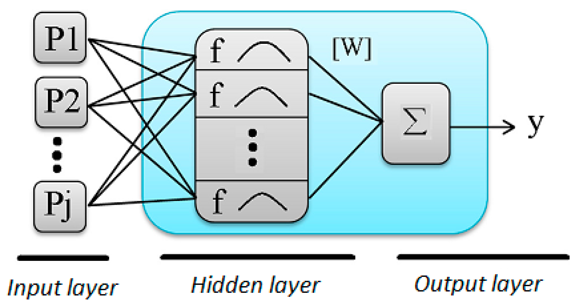
15]. Recently, a new category of models has been proposed based on soft computing methods, such as artificial neural networks, generic algorithms, and fuzzy logic. Models in this category can handle complex databases containing a large number of independent variables, identify the sensitivity of input parameters, and provide mathematical solutions between dependent and independent variables [16]. Pham and Hadi [16] proposed the utilization of neural networks to compute the strain and compressive strength of FRP-confined columns, and the results show agreement between proposed neural network models and experimental data. Also, there are several studies related to design-oriented and analysis-oriented models [9,17,18,19,20,21,22,23,24,25,26,27,28,29].
Lim et al. [30] proposed a new model for evaluating the ultimate condition of FRP-confined concrete using genetic programming (GP). The model was the first to establish the ultimate axial strain and hoop rupture strain expressions for FRP-confined concrete on the basis of evolutionary algorithms. The results showed that the predictions from the suggested model aligned with a database compiled by the authors. The proposed models provided improved predictions compared to the existing artificial intelligence models. The model proved that more accurate results can be achieved in explaining and formulating the ultimate condition of FRP-confined concrete. The model assessment presented in that study clearly illustrated the importance of the size of the test databases and the selected test parameters used in the development of artificial intelligence models on their overall performance.
This paper studies the capability of four soft computing techniques for predicting the ultimate strength and strain of FRP-confined concrete cylindrical specimens. The computing techniques include radial basis neural network (RBNN), adaptive neuro fuzzy inference system (ANFIS) with subtractive clustering (ANFIS-SC), ANFIS with fuzzy c-means clustering (ANFIS-FCM), and M5 model tree (M5Tree).

2. Overview of Soft Computing Approaches

2.1. Radial Basis Function Neural Network

Artificial neural networks (ANNs) are inspired by biological neural networks. ANNs include a set of processing components, called neurons, which operate in parallel processes and transmit information to other neurons, similar to the functioning of a biological brain. ANNs are an efficient method for modeling complex input-output relationships and can learn relationships directly from the data being modeled [31]. The nonlinearity within a radial basis function (RBF) network can be selected from a few classic nonlinear functions. The hidden layer carries out a fixed nonlinear transformation with no adjustable variables, and it maps the input onto a new layer. The output layer then performs a linear combination on this new layer, and the only adjustable variables are the weights of this linear combiner [32]. A general RBF network is schematically illustrated in Figure 1.
The radial basis function neural network (RBFN) model, which includes an input, an output and a single hidden layer, was developed by Powell [33] and Broomhead and Lowe [34]. In this model, the number of input and output nodes is similar to that of multi-layer perceptron (MLP) neural networks, and was selected using the nature of real input and output parameters. However, the rate of learning in RBFN is much faster than the MLP method. The output of RBFN can be calculated with the following equation:
Y = p = 1 p W p θ ( X X p )
In the equation, Wp is the weight connecting the output nodes and hidden nodes, θ represents the radial basis function, X and Y are the input and output variables, XP indicates the center of each hidden node which is dependent on the input data, and X X p represents the Euclidean metric between hidden and input nodes. Each group of input nodes which has identical information as the input is indicated by one hidden node, and the transformation related to any node within the hidden layer is named a Gaussian function [35]. More detailed information about RBNN theory can be obtained from Haykin [36].

2.2. Adaptive Neuro Fuzzy Inference System

ANFIS is a combined intelligent system including ideas from neural networks and fuzzy control, combining the advantages of both. Fuzzy logic is a superset of typical logic that has been improved to operate with uncertain data and the theory of partial truth [37,38]. The most important disadvantage of fuzzy logic is the lack of a systematic approach to choosing membership function variables and designing the fuzzy rules. On the other hand, ANN has the ability to learn its structure from the input-output sets.
Jang [39] introduced ANFIS as a universal approximation which can estimate any real continued function on a compact data set with the desired precision [40,41]. In terms of function, ANFIS can be considered as equivalent to fuzzy inference systems, and the ANFIS system used can be considered as comparable to the Sugeno first-order fuzzy model [42]. A simple example is presented below, in which a fuzzy inference system was assumed with two inputs of x and y and one output of z. For this example, the typical rule set of a first-order Sugeno fuzzy model, which possess two simple fuzzy If-Then rules, is as follows:
Rule 1 : IF x is A 1 , y is B 1 and z is C 1 THEN f 1 = p 1 x + q 1 y + r 1 z + t 1
Rule 2 : IF x is A 2 , y is B 2 and z is C 2 THEN f 2 = p 2 x + q 2 y + r 2 z + t 2
In the rule set, p1, q1, r1 and p2, q2, r2 are the variables of the THEN-part of the first-order Sugeno fuzzy model.
The ANFIS system uses a hybrid-learning algorithm to update parameters [43]. This algorithm is composed of two methods: the least squares approach and the gradient descent method. The function of the gradient descent approach is to adjust the variables of premise non-linear membership function, and the function of least squares method is to determine the resultant linear variables {pi, qi, ri}. The learning process of this system has two steps. The first step includes the identification of consequent variables by the least squares method, while the prior variables are assumed to be fixed for the running cycle by the training set. After that, the error signals will spread backwards. In this part, the function of the gradient descent method includes updating the premise variables by minimizing the cost function, while the resultant variables stay fixed. Jang [39] presented the details of this algorithm and mathematical foundations of the hybrid learning algorithm.
In the present paper, two different ANFIS methods, including ANFIS with subtractive clustering (ANFIS-SC) and ANFIS with fuzzy c-means clustering (ANFIS-FCM),are utilized as modeling techniques. Subtractive clustering (SC) is an extension of the mountain clustering method suggested by Yager and Filev [44]. In this method, the data are clustered by evaluating the potential of data in the specification space. FCM is the modified K-means algorithm; it has some restrictions and may not operate properly with large data sets. FCM minimizes within cluster variance and the classification of data using the clustering algorithm [45]. FCM works by minimizing the squared error function.

2.3. M5 Model Tree

Quinlan [46] explained the M5Tree, which includes a regression function at the terminal nodes. In fact, the M5 algorithm employs the idea of splitting the parameter space into subspaces and building a local linear regression model in each. The splitting follows the concept used in building a decision tree (see Figure 2).
The divide-and-conquer method is usually utilized to construct these types of tree-based models. Constructing a model tree entails two distinct steps. The first step includes a splitting criterion for the creation of a decision tree. In the M5Tree approach, this criterion is dependent on the standard deviation of the class values and then obtaining the decrement that can be expected in this error. The standard deviation reduction (SDR) can be calculated with the following equation:
S D R = s d ( T ) | T i | T s d ( T i )
In the equation, T indicates a set of instances that achieves the node, Ti is the subset of instances that have the ith result of the potential set, and sd is the standard deviation. The disarticulating proceeding causes the data in parent nodes to have more standard deviation compared to child nodes so that these data are purer. Once all the feasible splits are assessed, M5 selects the one that provides the maximum value for the expected error decrease. This grouping usually leads to a tree-like structure that should be trimmed by substituting a sub-tree, for example, with a leaf. In the next step, this tree growth must be trimmed and the sub-trees replaced with regression functions. In this method, the variable space is divided into several areas (subspaces), and a linear regression model is created for each of them. Quinlan [46] provides further details on M5Tree.

3. Results

In this study, four different soft computing techniques, i.e., RBNN, ANFIS-SC, ANFIS-FCM and M5 Tree, are employed for predicting strength ( f c c / f c o ) and strain (εcc/εco). For the model simulations, a MATLAB neural network and fuzzy tool boxes are used, and 519 experimental data are adopted from Sadeghian and Fam [48,49]. 
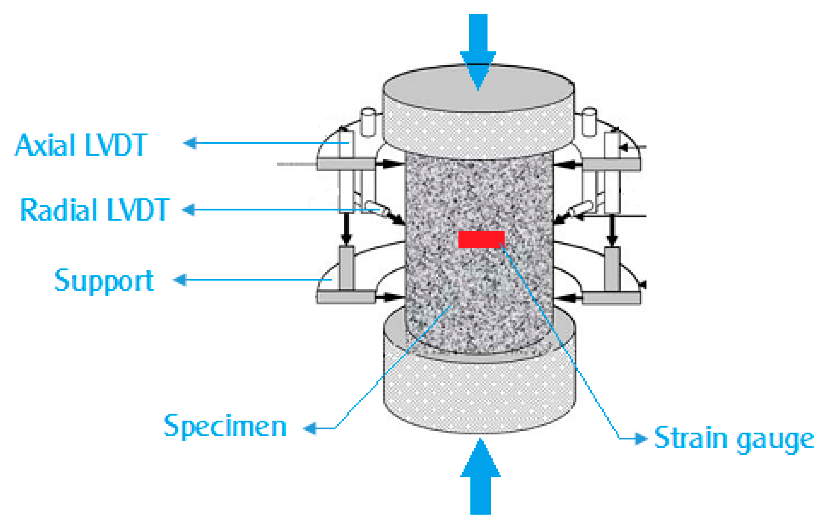
Figure 3 shows the usual test setup for confined cylinders. Also, the statistical analyses of the input data employed in this study are summarized in Table 1. The data are used to develop models for ultimate strength and strain based on the strain ratio (ρє) and the confinement stiffness ratio (ρK) inputs, which are defined as follows [48]:
f l = ρ K ρ ε f c o = 2 E f ε h , r u p t D
ρ K = 2 E f t ( f c o / ε c o ) D
ρ ε = ε h , r u p ε c o
In the equations, f c o is the unconfined concrete strength, εco is the corresponding axial strain of f c o , Ef is the elastic modulus of the FRP wrap in the hoop direction, t is the total thickness of the FRP wrap, εh,rup is the actual hoop rupture strain of the FRP wrap, and D is the diameter of the concrete core. The confinement ratio (fl/ f c o ) is a frequently used parameter in existing confinement models, which is equal to the product of ρK and ρε. Several equations have been proposed for estimating the strain and strength of FRP-confined concrete cylinders which depend on ρK and ρε [9,48]. According to Teng et al. [11], instead of the more approximate value of 0.002 for εco, it is assumed as follows:
ε c o = 9.37 × 10 4 f c o 4 , f c o i n M P a
The data set is randomly grouped into two subsets; the first data set is adopted for training, and the second data set (20% of the whole database) is adopted for the testing stage. Before application of the RBNN, the training values of input and output are normalized between 0.2 and 0.8 as follows:
b 1 x i x min x max x min + b 2
In the equation, xmax and xmin are the maximum and minimum values of the training data. Here values of 0.6 and 0.2 are respectively assigned for b1 and b2, and the input data are normalized within a range of 0.2 to 0.8, as recommended in Cigizoglu [51]. According to that study, input parameters ranging from 0.2 to 0.8 allow the artificial neural network the flexibility to appraise beyond the training range.
The applied models are compared with the mean absolute relative error (MARE), root mean square error (RMSE) and determination coefficient (R2). The definitions of statistical parameters are given as follows:
R M S E = 1 N i = 1 N ( X o i X e i ) 2
M A R E = 1 N i = 1 N | X o i X e i | X o i × 100
where N, Xoi and Xei are the number of samples, and the observed and estimated values, respectively.

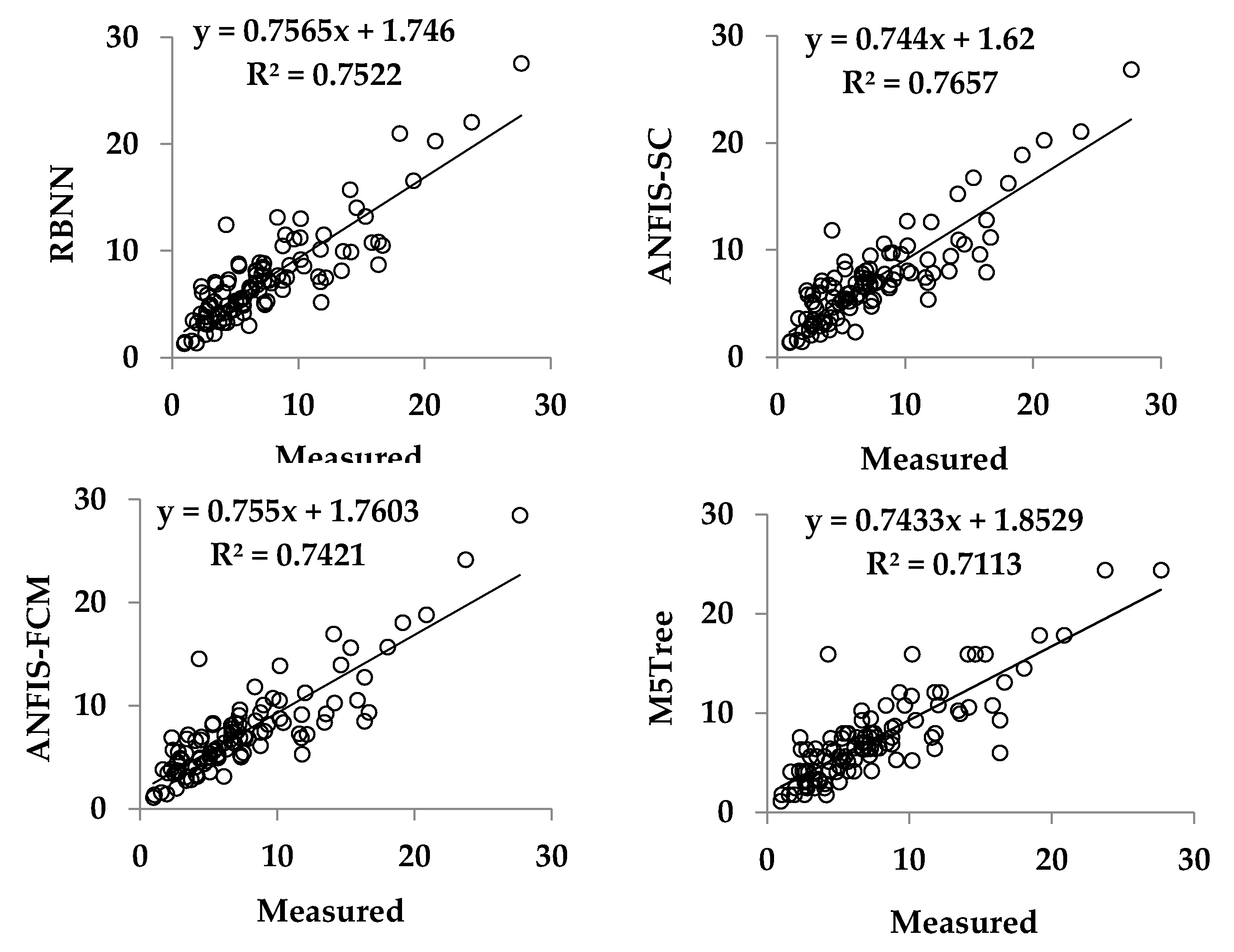
3.1. Ultimate Strength Prediction

Testing and training results for the prediction of strength of the RBNN, ANFIS-SC, ANFIS-FCM and M5Tree models are listed in Table 2. The control parameter values of the optimal models are also provided in the second column. Different numbers of parameters and structures were tried for each method and the optimal ones were selected. Gaussian membership functions are used in ANFIS-SC and ANFIS-FCM models. The RBNN, ANFIS-SC and ANFIS-FCM methods can be easily obtained and applied by using new RBNN, genfis2 and genfis3 tools in MATLAB command windows. For the M5Tree method, code which is available for free online (http://www.cs.rtu.lv/jekabsons/regression.html) is used.
In the table, 0.8 and 15 indicate the spread value and the number of hidden layer neuron of the RBNN model, respectively, while 0.1 and 10 show the radii and cluster number of the ANFIS-SC and ANFIS-FCM models. A radii value of 0.1 in ANFIS-FCM corresponds to 15 clusters. This means that the ANFIS-FCM has fewer membership functions and parameters (10 Gaussian membership function each have 2 parameters, or 20 parameters in total) than those of ANFIS-SC. Table 2 implies that RBNN and ANFIS-FCM have almost the same accuracy, and they both are more efficient than the ANFIS-SC and M5Ttree models with respect to RMSE, MARE and R2. It is interesting that the M5Tree approximated training data very well whereas its test results are worse than those of the other models. This implies that this method cannot adequately learn the investigated phenomenon. Different statistical indices were obtained for each of the methods. The main reason for this may be the fact that each method has different assumptions in developing models and their behaviors with the used data are distinct from each other. The rule base of the optimal ANFIS-FCM model is given in Table 3.
Table 3 demonstrates that the model has 10 clusters and one rule for each of them. Figure 4 illustrates the strength estimates of the applied models in the forms of time variation and scatterplot.
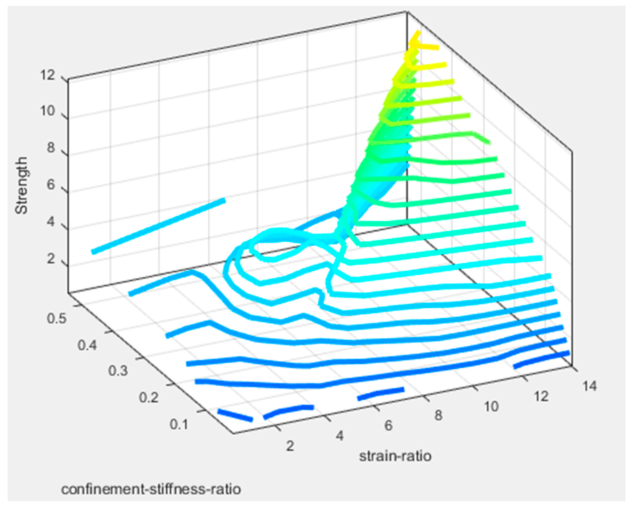
From the figure, it is apparent that the RBNN and ANFIS-FCM models have less scattered assessments than other models, and the M5Tree model gave the most scattered estimates. This reveals that the investigated phenomenon is nonlinear, and therefore linear M5Tree cannot adequately simulate strength behavior. The variation of strength versus strain ratio and confinement stiffness ratio for the optimal ANFIS-FCM model is illustrated in Figure 5, in which it is clear that strength takes its maximum value when the strain ratio is also at its maximum.
The linear behavior for a confinement-stiffness-ratio greater than 0.3 is observed in Figure 5. This is because of the exponent of the confinement-stiffness-ratio in equations is usually 0.7; therefore, values greater than 0.30.7 behave linearly.

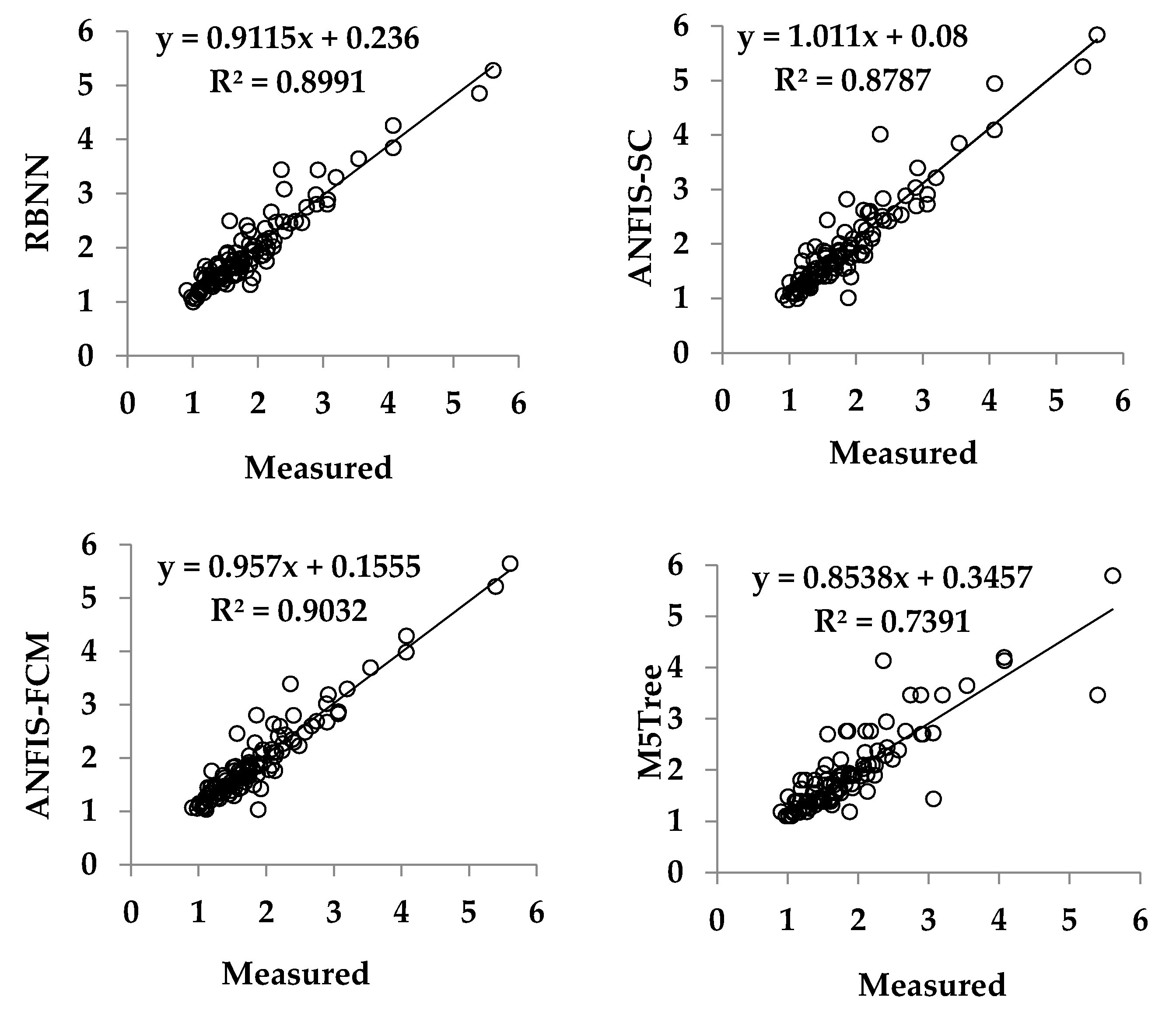
3.2. Ultimate Strains Prediction

Strain predictions for the RMSE, MARE and R2 values of the applied models are compared in Table 4.
This tables shows that the ANFIS-SC models outperform other models. Here also RBNN and ANFIS-FCM have similar accuracy, and they are slightly worse than the ANFIS-SC model. A radii value of 0.1 in ANFIS-SC corresponds to 13 clusters. Similar to the previous application, here too ANFIS-SC has many more membership functions and parameters compared to ANFIS-FCM. Table 5 gives the rule base of the optimal ANFIS-SC model. The estimated results of the optimal RBNN, ANFIS-FCM and ANFIS-SC models are shown in Figure 6.
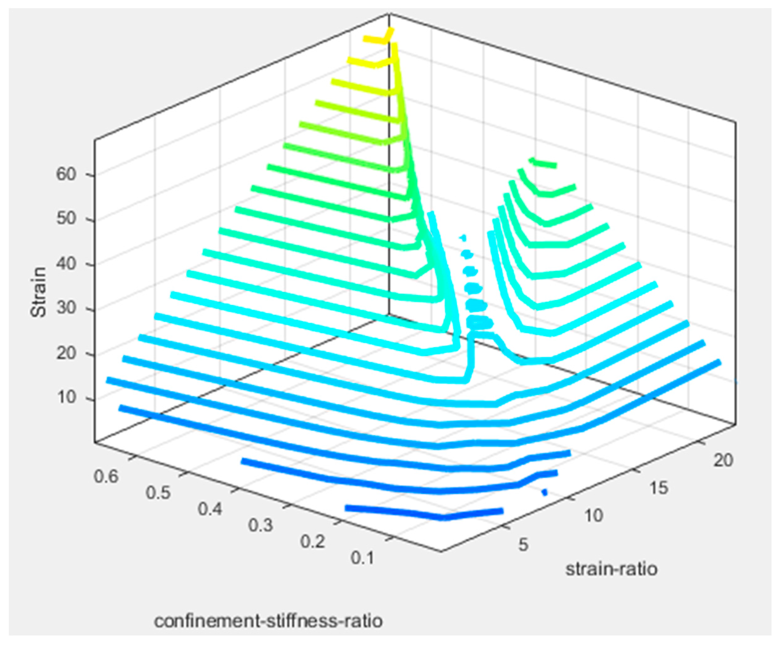
This figure shows that the estimates of the ANFIS-SC model are closer to the corresponding measured values, especially for high strain values. The variation of strength versus strain ratio and confinement stiffness ratio for the optimal ANFIS-SC model is shown in Figure 7. It is clear from the figure that strain takes its maximum value when the strain ratio and confinement stiffness ratio are both at their maximum values. The linear relationship between strain and strain ratio is clearly seen in the range of confinement-stiffness-ratio between 0.4 and 0.6.
The effects of strain ratio and the confinement stiffness ratio inputs on strength and strain were also investigated using the ANFIS-SC method because it has less control parameters than RBNN. For the RBNN models, the optimal radii and hidden node numbers should be determined whereas, in obtaining ANFIS-SC model, the radii value which indicates the number of clusters is only distinguished. The simulation results of the ANFIS-SC models are reported in Table 6.
This table indicates that the effect of ρK is more significant than ρє in strength and strain. The relative RMSE differences between ρK and ρє based ANFIS-SC models are 19.4% and 1.7% for strength and strain, respectively.
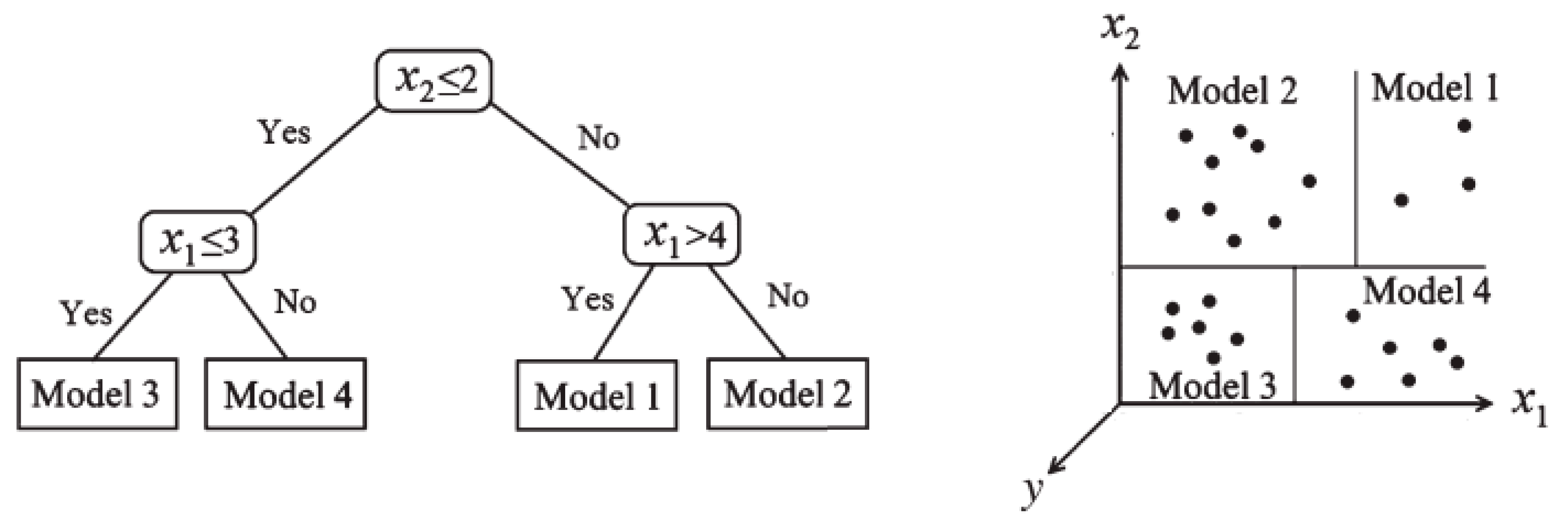
It should be noted that providing explicit formulation for the RBNN, ANFIS-SC and ANFIS-FCM is impossible because they are black-box models. However, the regression tree of the optimal M5Tree models for the strain and strength modeling are provided in Appendix A.

4. Conclusions

In this paper, the ultimate strength and strain of cylindrical concrete specimens confined with FRP composites were studied using four soft computational methods. The optimal RBNN, ANFIS-SC, ANFIS-FCM and M5Tree models obtained by trying different control parameters were compared with respect to RMSE, MARE and R2 statistics. RBNN and ANFIS-FCM provided almost the same level of accuracy, and they performed better than the other models in estimating strength of FRP-confined concrete cylindrical specimens by using the inputs of strain ratio and the confinement stiffness ratio. In estimating strain of FRPs, however, the ANFIS-SC model performed slightly better than the RBNN and ANFIS-FCM models. Among the applied models, the M5Tree model was the least accurate at estimating strength and strain of FRPs. The effects of strain ratio and the confinement stiffness ratio inputs on strength and strain were also examined using ANFIS-SC, and the confinement stiffness ratio was found to be more significant than strain ratio in strength and strain.

Acknowledgments

This research was supported by the Basic Science Research Program through the National Research Foundation of Korea (NRF), which is funded by the Ministry of Science, ICT & Future Planning of the Republic of Korea (2017R1A2B2010120).

Author Contributions

Pedram Sadeghian conceived and designed the database; Ozgur Kisi and Iman Mansouri analyzed the data; Jong Wan Hu and Iman Mansouri wrote the paper. Chang-Hwan Lee also analyzed the data and handled the final proofreading.

Conflicts of Interest

The authors declare no conflict of interest.

Appendix A. Regression Tree of the Optimal M5Tree Models for the Strain and Strength Modeling

Table A1. Regression tree obtained from M5Tree for strength modeling.
if x2 <= 0.065174   else if x2 <= 0.034551else if x1 <= 6.6355
 if x2 <= 0.0255    if x2 <= 0.033937 if x2 <= 0.15871
 if x1 <= 2.9025    y = 1.71921529875 (4)  if x1 <= 3.3762
  if x1 <= 2.505   else  if x2 <= 0.071835
  y = 1.108064681 (10)    y = 1.92418515966667 (6)   y = 1.55785802183333 (6)
  else   else if x2 <= 0.037414  else if x1 <= 2.6111
  y = 0.891721241833333 (6)    y = 1.45295335707692 (13)   y = 1.8102727921 (20)
 else if x2 <= 0.021267    else if x2 <= 0.044137   else
  if x2 <= 0.010372     y = 1.73181401571429 (14)   y = 1.57794946244278 +4.99230783389806*x2 (11)
   y = 1.483590448 (4)    else if x2 <= 0.045434  else if x2 <= 0.092595
  else if x2 <= 0.015328     y = 1.41987727225 (4)   if x2 <= 0.06805
   y = 1.13560753725 (12)     else   if x2 <= 0.066642
   else if x2 <= 0.018965     y = 1.587916394 (4)    y = 2.34944086616667 (6)
    y = 1.25916023821429 (14)  else if x1 <= 3.7759   else
   else   y = 1.64059121775 (4)    y = 2.7420408164 (5)
   y = 1.1897478106 (5)   else if x2 <= 0.056561   else if x2 <= 0.074024
  else if x1 <= 6.5213    if x2 <= 0.04728    y = 1.9024165688 (5)
   if x1 <= 4.9928    y = 1.7582115855 (4)   else
   y = 1.26759138458333 (12)    else if x2 <= 0.050345    y = 2.10530567306667 (15)
   else     y = 2.23252585925 (4)else if x1 <= 3.9987
   y = 1.3995581252 (5)    else   y = 5.07504348861174 -23.5904126567999*x2 (11)
  else if x1 <= 7.387     y = -4.7981786875333 +124.346272222065*x2 (9)   else if x2 <= 0.10281
   y = 1.654221567 (4)   else    y = 2.9481859308 (5)
   else    y = 2.72437967584461 - 0.199395562322418*x1 (13)   else
   y = 1.4358405485 (4) else if x2 <= 0.049162    y = 2.70621362185714 (7)
 else if x1 <= 7.0025  if x2 <= 0.037766 else if x1 <= 2.9764
  if x1 <= 3.4344   if x1 <= 8.8613  y = 2.767153359 (19)
  if x2 <= 0.029531   if x2 <= 0.033956  else if x2 <= 0.22102
   y = 1.16075967033333 (6)    y = 1.7132418315 (12)   y = 3.47170636066667 (9)
  else if x1 <= 1.3994   else  else
   y = 1.179568198 (4)    y = 1.89220380857143 (7)   y = 4.1398758346 (5)
   else if x2 <= 0.059018   elseelse if x2 <= 0.13591
    y = 1.39728594933333 (24)   y = 2.15360432216667 (6)  if x2 <= 0.068264
   else  else  y = 2.72699884416667 (6)
    y = 1.59811338542857 (7)   y = 2.21282843818182 (11)  else if x2 <= 0.1031
  else if x2 <= 0.04595  else if x1 <= 7.8378   y = 3.65529982828571 (7)
   if x2 <= 0.033094   y = 2.3919454476 (5)  else
   if x1 <= 5.5058  else   y = 4.204802991 (4)
    y = 1.323997823 (12)   y = 2.915657196 (7) else
    else   y = 1.45436334578442 +23.9129270980071*x2 (10)
    y = 1.56201983057143 (7)
Table A2. Regression tree obtained from M5Tree for strain modeling.
if x1 <= 6.2548    else   else
 if x2 <= 0.06311    y = 4.69127474228571 (7)    y = 6.0040160536 (5)
 if x1 <= 3.6413   else  else if x2 <= 0.20919
  if x2 <= 0.020455    y = 6.3533113762 (5)   y = 2.39097472537744 +2.19876304626978*x1 (10)
  if x1 <= 1.8874  else if x1 <= 5.6305  else
   y = 1.1440491595 (6)    if x1 <= 4.5915   y = 14.51223043 (8)
  else    if x2 <= 0.038697else if x2 <= 0.05346
   y = 1.68687631466667 (9)     y = 5.82153494575 (4) if x2 <= 0.022672
  else if x1 <= 2.6807    else if x2 <= 0.055755  y = 3.41272976260672 +0.218464713423608*x1 (22)
   if x1 <= 2.2516     y = 7.6093721018 (5) else if x1 <= 8.8613
   if x1 <= 1.7107     else  if x2 <= 0.033956
    y = 1.78844272172727 (11)     y = 6.4901269452 (5)   y = 11.8427843384812 -146.164747121597*x2 (20)
   else    else  else if x2 <= 0.035225
    y = 3.15371412385714 (7)    y = 6.42120672495833 (24)   y = 12.096092072 (5)
   else   else   else if x2 <= 0.041997
   y = 1.764552396 (6)    y = 8.64814412742857 (7)    if x1 <= 7.2822
  else if x2 <= 0.047075 else if x1 <= 2.8545    y = 5.2413583345 (4)
   if x2 <= 0.035327  if x2 <= 0.14161    else
    if x1 <= 3.4003  if x1 <= 0.94068    y = 8.69478460875 (4)
    y = 2.8827251381 (10)   y = 1.6541689808 (5)   else
    else  else if x2 <= 0.12452    y = 10.7816929114 (10)
    y = 4.1709103866 (5)   if x2 <= 0.091846  else
   else    y = 3.8282330848 (10)  y = -4.15948380355076 +1.79907971888928*x1 (8)
    y = 3.072717053875 (8)   else else if x2 <= 0.14656
   else    y = 5.62676665785714 (7)  if x1 <= 7.7892
   y = 4.18276414975 (12)   else  if x2 <= 0.067874
 else if x2 <= 0.021073   y = 3.269071034 (4)   y = 11.774363725 (6)
  if x2 <= 0.018742  else  else
   y = 2.46492040855556 (9)  y = 7.55286884866667 (21)   y = 15.9303924215 (8)
  else else if x2 <= 0.14818  else
   y = 3.35411568575 (4)  if x2 <= 0.092595  y = 17.838992625 (18)
  else if x1 <= 4.0509   if x1 <= 4.2573 else
   if x2 <= 0.054126   if x1 <= 3.429  y = 24.3989610371429 (7)
   y = 4.0987042836 (15)    y = 7.9752687216 (5)  else if x2 <= 0.11185
   else   else   y = 10.2661860479091 (11)
   y = 6.1883060684 (5)    y = 10.9299345495055 -67.7789156702637*x2 (13)   else if x1 <= 4.1077
  else if x2 <= 0.033258   else if x1 <= 5.2858    y = 6.97833482855556 (9)
   if x1 <= 5.6609    if x1 <= 4.3562   else
    if x2 <= 0.024021    y = 7.779023415 (4)    y = 9.9430306388 (5)
    y = 6.21866667766667 (6)    else
    else if x2 <= 0.029178    y = 9.292927947 (10)
     y = 2.6673381094 (5)

References

  1. Green, M.F.; Bisby, L.A.; Fam, A.Z.; Kodur, V.K.R. Frp confined concrete columns: Behaviour under extreme conditions. Cem. Concr. Compos. 2006, 28, 928–937. [Google Scholar] [CrossRef]
  2. Mirmiran, A.; Shahawy, M.; Samaan, M.; El Echary, H.; Mastrapa, J.C.; Pico, O. Effect of column parameters on frp-confined concrete. J. Compos. Constr. 1998, 2, 175–185. [Google Scholar] [CrossRef]
  3. Nanni, A.; Bradford, N.M. Frp jacketed concrete under uniaxial compression. Constr. Build. Mater. 1995, 9, 115–124. [Google Scholar] [CrossRef]
  4. Pessiki, S.; Harries, K.A.; Kestner, J.T.; Sause, R.; Ricles, J.M. Axial behavior of reinforced concrete columns confined with frp jackets. J. Compos. Constr. 2001, 5, 237–245. [Google Scholar] [CrossRef]
  5. Sadeghian, P.; Rahai, A.R.; Ehsani, M.R. Effect of fiber orientation on compressive behavior of cfrp-confined concrete columns. J. Reinf. Plast. Compos. 2010, 29, 1335–1346. [Google Scholar] [CrossRef]
  6. Mansouri, I.; Gholampour, A.; Kisi, O.; Ozbakkaloglu, T. Evaluation of peak and residual conditions of actively confined concrete using neuro-fuzzy and neural computing techniques. Neural Comput. Appl. 2016, 1–16. [Google Scholar] [CrossRef]
  7. Mansouri, I.; Ozbakkaloglu, T.; Kisi, O.; Xie, T. Predicting behavior of frp-confined concrete using neuro fuzzy, neural network, multivariate adaptive regression splines and m5 model tree techniques. Mater. Struct. Materiaux Constr. 2016, 49, 4319–4334. [Google Scholar] [CrossRef]
  8. Karbhari, V.M.; Gao, Y. Composite jacketed concrete under uniaxial compression—Verification of simple design equations. J. Mater. Civ. Eng. 1997, 9, 185–193. [Google Scholar] [CrossRef]
  9. Lam, L.; Teng, J.G. Design-oriented stress-strain model for frp-confined concrete. Constr. Build. Mater. 2003, 17, 471–489. [Google Scholar] [CrossRef]
  10. Samaan, M.; Mirmiran, A.; Shahawy, M. Model of concrete confined by fiber composites. J. Struct. Eng. 1998, 124, 1025–1031. [Google Scholar] [CrossRef]
  11. Teng, J.G.; Jiang, T.; Lam, L.; Luo, Y.Z. Refinement of a design-oriented stress-strain model for frp-confined concrete. J. Compos. Constr. 2009, 13, 269–278. [Google Scholar] [CrossRef]
  12. Toutanji, H.A. Stress-strain characteristics of concrete columns externally confined with advanced fiber composite sheets. ACI Mater. J. 1999, 96, 397–404. [Google Scholar]
  13. Harries, K.A.; Kharel, G. Behavior and modeling of concrete subject to variable confining pressure. ACI Mater. J. 2002, 99, 180–189. [Google Scholar]
  14. Spoelstra, M.R.; Monti, G. Frp-confined concrete model. J. Compos. Constr. 1999, 3, 143–150. [Google Scholar] [CrossRef]
  15. Fam, A.Z.; Rizkalla, S.H. Confinement model for axially loaded concrete confined by circular fiber-reinforced polymer tubes. ACI Struct. J. 2001, 98, 451–461. [Google Scholar]
  16. Pham, T.M.; Hadi, M.N.S. Predicting stress and strain of frp-confined square/rectangular columns using artificial neural networks. J. Compos. Constr. 2014, 18, 1–9. [Google Scholar] [CrossRef]
  17. Berthet, J.F.; Ferrier, E.; Hamelin, P. Compressive behavior of concrete externally confined by composite jackets: Part b: Modeling. Constr. Build. Mater. 2006, 20, 338–347. [Google Scholar] [CrossRef]
  18. Bisby, L.A.; Dent, A.J.S.; Green, M.F. Comparison of confinement models for fiber-reinforced polymer-wrapped concrete. ACI Struct. J. 2005, 102, 62–72. [Google Scholar]
  19. Cascardi, A.; Micelli, F.; Aiello, M.A. Unified model for hollow columns externally confined by frp. Eng. Struct. 2016, 111, 119–130. [Google Scholar] [CrossRef]
  20. Cascardi, A.; Micelli, F.; Aiello, M.A. An artificial neural networks model for the prediction of the compressive strength of frp-confined concrete circular columns. Eng. Struct. 2017, 140, 199–208. [Google Scholar] [CrossRef]
  21. Faustino, P.; Chastre, C. Analysis of load–strain models for rc square columns confined with cfrp. Compos. Part B Eng. 2015, 74, 23–41. [Google Scholar] [CrossRef]
  22. Ilki, A.; Kumbasar, N.; Koc, V. Low strength concrete members externally confined with frp sheets. Struct. Eng. Mech. 2004, 18, 167–194. [Google Scholar] [CrossRef]
  23. Matthys, S.; Toutanji, H.; Audenaert, K.; Taerwe, L. Axial load behavior of large-scale columns confined with fiber-reinforced polymer composites. ACI Struct. J. 2005, 102, 258–267. [Google Scholar]
  24. Naderpour, H.; Kheyroddin, A.; Amiri, G.G. Prediction of frp-confined compressive strength of concrete using artificial neural networks. Compos. Struct. 2010, 92, 2817–2829. [Google Scholar] [CrossRef]
  25. Rousakis, T.C.; Tourtouras, I.S. Modeling of passive and active external confinement of rc columns with elastic material. ZAMM J. Appl. Math. Mech. 2015, 95, 1046–1057. [Google Scholar] [CrossRef]
  26. Saiidi, M.S.; Kandasamy, S.; Claudia, P. Simple carbon-fiber-reinforced-plastic-confined concrete model for moment-curvature analysis. J. Compos. Constr. 2005, 9, 101–104. [Google Scholar] [CrossRef]
  27. Sidney, A.G.; Lukito, G. Strengthening of reinforced concrete bridge columns with frp wrap. Pract. Period. Struct. Des. Constr. 2006, 11, 218–228. [Google Scholar]
  28. Tamuzs, V.; Tepfers, R.; Sparnins, E. Behavior of concrete cylinders confined by carbon composite 2. Prediction of strength. Mech. Compos. Mater. 2006, 42, 109–118. [Google Scholar] [CrossRef]
  29. Teng, J.G.; Lin, G.; Yu, T. Analysis-oriented stress-strain model for concrete under combined frp-steel confinement. J. Compos. Constr. 2015, 19. [Google Scholar] [CrossRef]
  30. Lim, J.C.; Karakus, M.; Ozbakkaloglu, T. Evaluation of ultimate conditions of frp-confined concrete columns using genetic programming. Comput. Struct. 2016, 162, 28–37. [Google Scholar] [CrossRef]
  31. Zounemat-kermani, M.; Kisi, O.; Rajaee, T. Performance of radial basis and lm-feed forward artificial neural networks for predicting daily watershed runoff. Appl. Soft Comput. 2013, 13, 4633–4644. [Google Scholar] [CrossRef]
  32. Senthil Kumar, A.R.; Ojha, C.S.P.; Goyal, M.K.; Singh, R.D.; Swamee, P.K. Modeling of suspended sediment concentration at kasol in india using ann, fuzzy logic, and decision tree algorithms. J. Hydrol. Eng. 2012, 17, 394–404. [Google Scholar] [CrossRef]
  33. Powell, M.J.D. Radial basis functions for multivariable interpolation: A review. In Proceedings of the IMA Conference on Algorithms for the Approximation of Functions and Data, RMCS, Shrivenham, UK, 1–30 July 1987; pp. 143–167. [Google Scholar]
  34. Broomhead, D.S.; Lowe, D. Multivariable functional interpolation and adaptive networks. Complex Syst. 1988, 2, 321–355. [Google Scholar]
  35. Rezaeian-Zadeh, M.; Zand-Parsa, S.; Abghari, H.; Zolghadr, M.; Singh, V.P. Hourly air temperature driven using multi-layer perceptron and radial basis function networks in arid and semi-arid regions. Theor. Appl. Climatol. 2012, 109, 519–528. [Google Scholar] [CrossRef]
  36. Haykin, S. Neural Networks and Learning Machines, 3rd ed.; Prentice Hall: New Jersey, NJ, USA, 2008. [Google Scholar]
  37. Deka, P.; Chandramouli, V. Fuzzy neural network model for hydrologic flow routing. J. Hydrol. Eng. 2005, 10, 302–314. [Google Scholar] [CrossRef]
  38. Yilmaz, A.G.; Muttil, N. Runoff estimation by machine learning methods and application to the euphrates basin in Turkey. J. Hydrol. Eng. 2014, 19, 1015–1025. [Google Scholar] [CrossRef]
  39. Jang, J.S.R. Anfis: Adaptive-network-based fuzzy inference system. IEEE Transact. Syst. Man Cybern. 1993, 23, 665–685. [Google Scholar] [CrossRef]
  40. Jang, J.S.R.; Sun, C.T.; Mizutani, E. Neuro-Fuzzy and Soft Computing: A Computational Approach to Learning and Machine Intelligence; Prentice-Hall Upper Saddle River: New Jersey, NY, USA, 1997. [Google Scholar]
  41. Mansouri, I.; Kisi, O. Prediction of debonding strength for masonry elements retrofitted with frp composites using neuro fuzzy and neural network approaches. Compos. Part B Eng. 2015, 70, 247–255. [Google Scholar] [CrossRef]
  42. Drake, J.T. Communications Phase Synchronization Using the Adaptive Network Fuzzy Inference System. Ph.D. Thesis, New Mexico State University, Albuquerque, NM, USA, 2000. [Google Scholar]
  43. Mansouri, I.; Shariati, M.; Safa, M.; Ibrahim, Z.; Tahir, M.M.; Petković, D. Analysis of influential factors for predicting the shear strength of a v-shaped angle shear connector in composite beams using an adaptive neuro-fuzzy technique. J. Intell. Manuf. 2017, 28, 1–11. [Google Scholar] [CrossRef]
  44. Yager, R.R.; Filev, D.P. Approximate clustering via the mountain method. IEEE Transact. Syst. Man Cybern. 1994, 24, 1279–1284. [Google Scholar] [CrossRef]
  45. Ayvaz, M.T.; Karahan, H.; Aral, M.M. Aquifer parameter and zone structure estimation using kernel-based fuzzy c-means clustering and genetic algorithm. J. Hydrol. 2007, 343, 240–253. [Google Scholar] [CrossRef]
  46. Quinlan, J.R. Learning with continuous classes. In Proceedings of the 5th Australian Joint Conference on Artificial Intelligence (AI ’92), Hobart, Australia, 16–18 October 1992; Adams, A., Sterling, L., Eds.; World Scientific Publishing: Singapore, 1992; pp. 343–348. [Google Scholar]
  47. Wang, L.; Kisi, O.; Zounemat-Kermani, M.; Zhu, Z.; Gong, W.; Niu, Z.; Liu, H.; Liu, Z. Prediction of solar radiation in China using different adaptive neuro-fuzzy methods and m5 model tree. Int. J. Climatol. 2017, 37, 1141–1155. [Google Scholar] [CrossRef]
  48. Sadeghian, P.; Fam, A. Improved design-oriented confinement models for frp-wrapped concrete cylinders based on statistical analyses. Eng. Struct. 2015, 87, 162–182. [Google Scholar] [CrossRef]
  49. Sadeghian, P.; Fam, A. A rational approach toward strain efficiency factor of fiber-reinforced polymer-wrapped concrete columns. ACI Struct. J. 2014, 111, 135–144. [Google Scholar]
  50. Berthet, J.F.; Ferrier, E.; Hamelin, P. Compressive behavior of concrete externally confined by composite jackets. Part a: Experimental study. Constr. Build. Mater. 2005, 19, 223–232. [Google Scholar] [CrossRef]
  51. Cigizoglu, H.K. Estimation, forecasting and extrapolation of river flows by artificial neural networks. Hydrol. Sci. J. 2003, 48, 349–362. [Google Scholar] [CrossRef]
Figure 1. Schematic of a RBF network [31].
Applsci 07 00751 g001
Figure 2. M5 tree; splitting the input space into subspaces and the resultant diagram [47].
Applsci 07 00751 g002
Figure 3. Test setup and instrumentation [50].
Applsci 07 00751 g003
Figure 4. Strength estimates of the RBNN, ANFIS-SC, ANFIS-FCM and M5Tree models (dimensionless: f c c / f c o ).
Applsci 07 00751 g004
Figure 5. Variation of strength versus strain ratio and confinement stiffness ratio for the optimal ANFIS-FCM model.
Applsci 07 00751 g005
Figure 6. Strain estimates of the RBNN, ANFIS-SC, ANFIS-FCM and M5Tree models (dimensionless: εcc/εco).
Applsci 07 00751 g006
Figure 7. Variation of strain versus strain ratio and confinement stiffness ratio for the optimal ANFIS-SC model.
Applsci 07 00751 g007
Table 1. Statistics for the experimental data.
D (mm)t (mm) f c o (MPa) f c c (MPa)εco (%)εcc (%)εh,rup (%)ρεEf (GPa)ρK
Min. value51.000.0919.7031.400.200.230.100.2910.500.01
Max. value406.007.26188.20372.200.356.204.9823.03662.500.68
Average158.460.8946.5283.880.241.681.124.80183.090.07
Standard deviation52.741.0627.0542.180.031.050.532.44124.730.07
Table 2. Statistical performance of RBNN, ANFIS-SC, ANFIS-FCM and M5Tree models in strength predictions.
MethodControl ParametersTrainingTest
RMSEMARER2RMSEMARER2
RBNN0.8,150.3211.60.8800.2710.50.899
ANFIS-SC0.10.3111.10.8910.3211.30.879
ANFIS-FCM100.3011.00.8960.2710.70.903
M5Tree 0.268.250.9210.4314.30.739
Table 3. Rule base of the optimal ANFIS-FCM in modeling strength.
1.If (strain-ratio is in1cluster1) and (confinement-stiffness-ratio is in2cluster1) then (Strength is out1cluster1)
2.If (strain-ratio is in1cluster2) and (confinement-stiffness-ratio is in2cluster2) then (Strength is out1cluster2)
3.If (strain-ratio is in1cluster3) and (confinement-stiffness-ratio is in2cluster3) then (Strength is out1cluster3)
4.If (strain-ratio is in1cluster4) and (confinement-stiffness-ratio is in2cluster4) then (Strength is out1cluster4)
5.If (strain-ratio is in1cluster5) and (confinement-stiffness-ratio is in2cluster5) then (Strength is out1cluster5)
6.If (strain-ratio is in1cluster6) and (confinement-stiffness-ratio is in2cluster6) then (Strength is out1cluster6)
7.If (strain-ratio is in1cluster7) and (confinement-stiffness-ratio is in2cluster7) then (Strength is out1cluster7)
8.If (strain-ratio is in1cluster8) and (confinement-stiffness-ratio is in2cluster8) then (Strength is out1cluster8)
9.If (strain-ratio is in1cluster9) and (confinement-stiffness-ratio is in2cluster9) then (Strength is out1cluster9)
10.If (strain-ratio is in1cluster10) and (confinement-stiffness-ratio is in2cluster10) then (Strength is out1cluster10)
Table 4. Statistical performance of RBNN, ANFIS-SC, ANFIS-FCM and M5Tree models in strain predictions.
MethodControl ParametersTrainingTest
RMSEMARER2RMSEMARER2
RBNN0.6402.4329.90.7672.5131.60.752
ANFIS-SC0.12.3129.40.7902.4730.50.766
ANFIS-FCM62.3331.30.7862.5731.90.742
M5Tree 1.9021.80.8582.7233.30.711
Table 5. Rule base of the optimal ANFIS-SC in modeling strain.
1.If (strain-ratio is in1cluster1) and (confinement-stiffness-ratio is in2cluster1) then (Strength is out1cluster1)
2.If (strain-ratio is in1cluster2) and (confinement-stiffness-ratio is in2cluster2) then (Strength is out1cluster2)
3.If (strain-ratio is in1cluster3) and (confinement-stiffness-ratio is in2cluster3) then (Strength is out1cluster3)
4.If (strain-ratio is in1cluster4) and (confinement-stiffness-ratio is in2cluster4) then (Strength is out1cluster4)
5.If (strain-ratio is in1cluster5) and (confinement-stiffness-ratio is in2cluster5) then (Strength is out1cluster5)
6.If (strain-ratio is in1cluster6) and (confinement-stiffness-ratio is in2cluster6) then (Strength is out1cluster6)
7.If (strain-ratio is in1cluster7) and (confinement-stiffness-ratio is in2cluster7) then (Strength is out1cluster7)
8.If (strain-ratio is in1cluster8) and (confinement-stiffness-ratio is in2cluster8) then (Strength is out1cluster8)
9.If (strain-ratio is in1cluster9) and (confinement-stiffness-ratio is in2cluster9) then (Strength is out1cluster9)
10.If (strain-ratio is in1cluster10) and (confinement-stiffness-ratio is in2cluster10) then (Strength is out1cluster10)
11.If (strain-ratio is in1cluster11) and (confinement-stiffness-ratio is in2cluster11) then (Strength is out1cluster11)
12.If (strain-ratio is in1cluster12) and (confinement-stiffness-ratio is in2cluster12) then (Strength is out1cluster12)
13.If (strain-ratio is in1cluster13) and (confinement-stiffness-ratio is in2cluster13) then (Strength is out1cluster13)
Table 6. Effect of strain ratio (ρє) and the confinement stiffness ratio (ρK) inputs on strength and strain with respect to ANFIS-SC.
InputsControl ParametersTrainingTest
RMSEMARER2RMSEMARER2
Strength
ρє0.10.85232.80.2490.80432.80.054
ρK0.10.64621.30.5120.64825.10.445
Strain
ρє0.24.08163.60.3434.40659.20.244
ρK0.14.45371.80.2184.33063.20.265

