Development of a Fractional Order Chaos Synchronization Dynamic Error Detector for Maximum Power Point Tracking of Photovoltaic Power Systems

Abstract

In recent years, the photovoltaic (PV) power generation system has been widely discussed and researched. Research on electric energy focuses on the development of Maximum Power Point Tracking (MPPT) technology, and many methods have been proposed. However, these studies have a common defect: the tracking continues near the maximum power point (MPP), so that the waveform of output power jitters, thus causing power loss and rapid wearing of electronic modules. In order to remedy this defect, this paper proposes a new type of fractional order chaos synchronization dynamic error detector for the MPPT design of a PV power system. In this study, the Sprott chaos synchronization dynamic error system was used to control the pulse width duty cycle of PWM and optimize the power oscillation of a PV power system during steady-state response. The simulation and experimental results showed that the voltage detector proposed in this paper can reduce the power oscillation of a PV power system during steady-state response, and increase the overall system efficiency. From the steady-state responses of MPPT, it can be seen that about 0.2 vibration amplitude can be suppressed with control action. Therefore, about 4% of steady-state vibration energy can be saved.

1. Introduction

Alternative energy has become a topical subject in many countries in recent years, with solar energy emerging as a promising energy source since the radiant energy of the sun is inexhaustible. In recent years, this aspect of the development of the smart grid is booming [1]. Photovoltaic (PV) panels for solar power generation can convert solar radiant energy directly into electric energy. At present, the PV power system has not reached high conversion efficiency, requires high cost, and the power benefit varies with climatic conditions and ambient temperature. Therefore, how to maximize the power output of PV power system and reduce power waste has become an important topic.

Many Maximum Power Point Tracking (MPPT) technologies have been used in PV power systems in the literature [2], such as the voltage feedback method [3], the power feedback method, the incremental conductance method (INC) [4], and Perturbation and Observation (P&O) [5,6]. Otherwise, a hybrid MPPT technique proposed by Aurilio et al. [7] was applied in the MPPT of PV power system since it is neither only distributed on the PV modules of the PV array nor only centralized at the input of the inverter. The optimal scheme was used to estimate the optimal values of PV module voltages and the input inverter voltage. Therefore, the high speed of tracking of MPPT was obtained by this scheme. The tracking speed of general MPPT methods is determined by the step size, and continuous MPPT during steady-state response results in steady-state power oscillation, thereby causing power loss and wearing of electronic modules.

Most previous studies used decreasing steps to reduce the steady-state oscillations. However, the sampling time cannot be infinitely smaller due to the limits of physical elements in the real physical system. Therefore, how to reduce the steady-state oscillations in cases where the step sizes of MPPT cannot be reduced is an important issue.

Our previous study used fractional order incremental conductance method as the algorithm implement for MPPT [8]. This method has improved the transient tracking speed, but the oscillation during steady-state response is not improved completely. In order to avoid the PV system having power oscillation near the MPP, this study combines the fractional order chaos synchronization dynamic error detector with the MPPT control of fractional order incremental conductance method proposed in [8]. The proposed MPPT controller is combined with a voltage detector algorithm [9,10]. The voltage from the PV panels is captured and calculated by MPPT controller. The result is extracted to the chaos synchronization dynamic error detector to adjust the PWM signal to control the PWM duty ratio of DC/DC converter [11], as the framework of the overall PV power system.

The remainder of this study is organized as follows. Section 2 describes the existing problems and research motives; Section 3 presents the MPPT design and illustrates the voltage detector design; Section 4 discusses the simulation and experimental results. Finally, conclusions are drawn in Section 5.

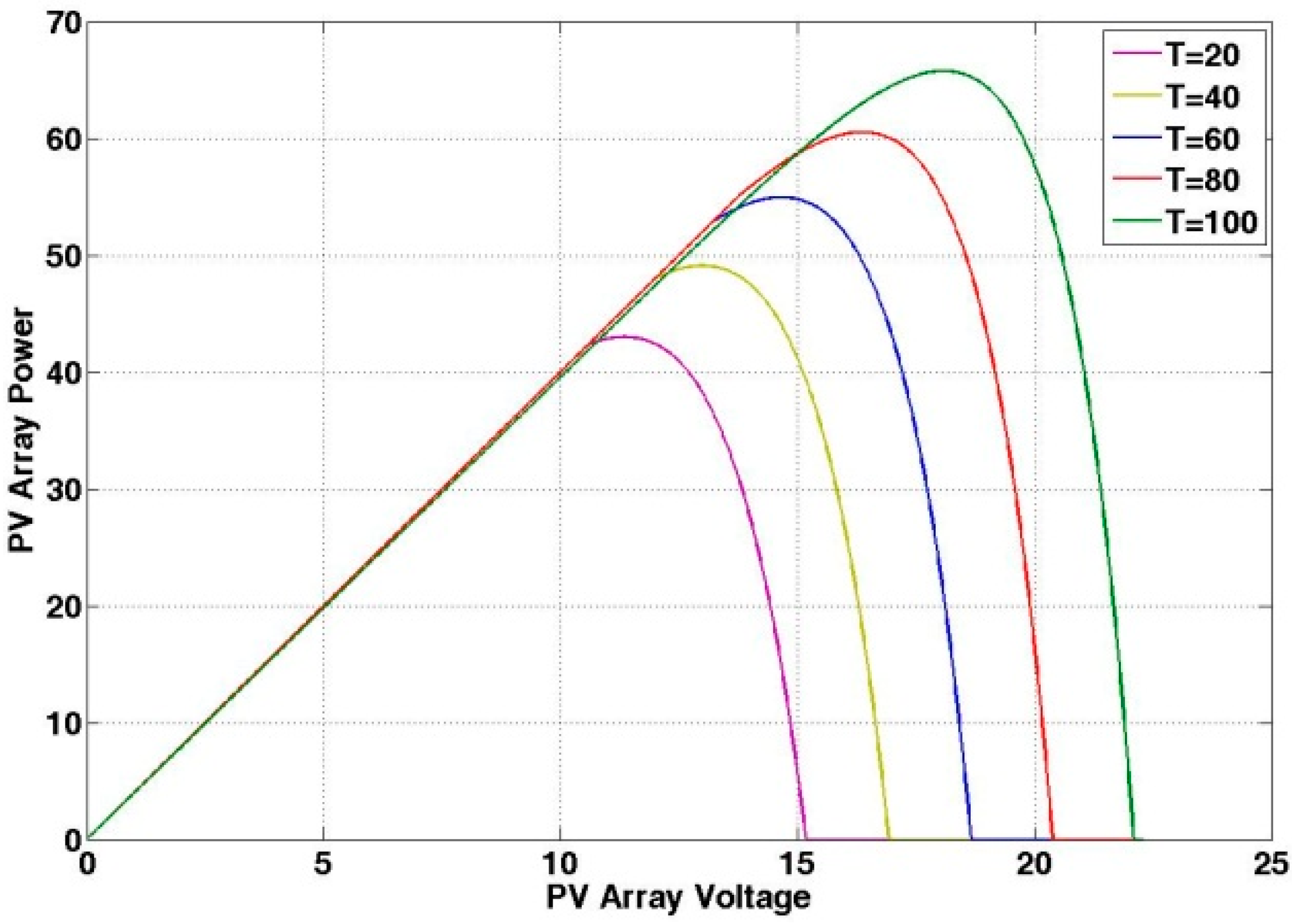
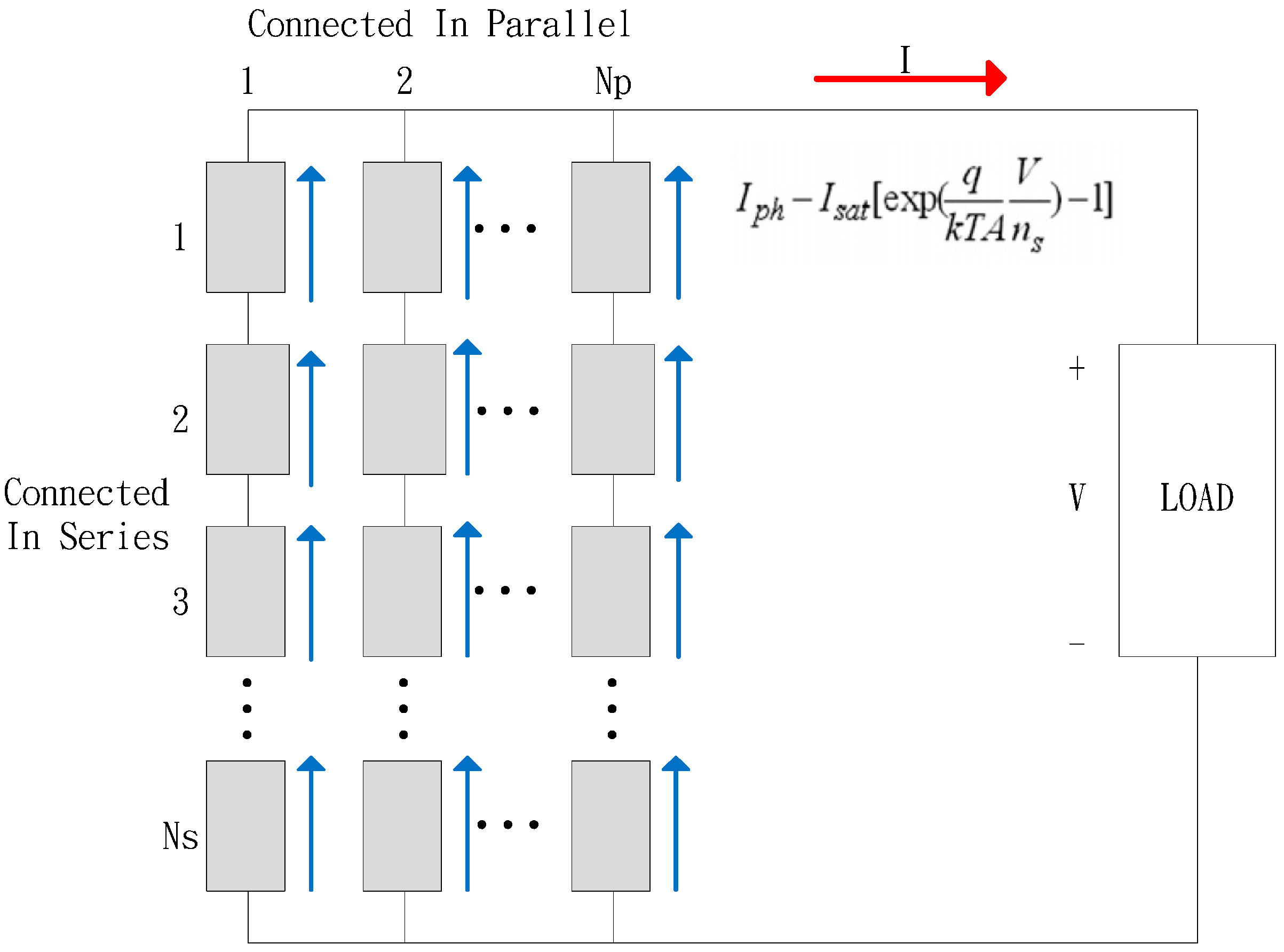
2. Problem Description and Motives

In terms of a solar cell, when the sun irradiates the P-N junction semiconductor, the electric energy is generated by the movement of electron holes. The PV panel consists of several solar cells in series-parallel connection, as shown in Figure 1. The output current can be expressed as Equation (1):

$$I=n_p{I}_{ph}-n_p{I}_{sat}[\exp (\frac{qV}{kTA{n}_s})-1],$$

(1)

where I is the output current of PV panel, V is the output voltage of PV panel, q is the electric quantity of electron, I_ph is the photocurrent, I_sat is the reverse saturation current, T is the cell temperature, n_p is the parallel number of PV panels, n_s is the serial number of PV panels, k is the Boltzmann constant, and A is the ideal factor coefficient of PN junction. When I_sat and I_ph are sensitive to the cell temperature, this is expressed as Equations (2) and (3):

$$I_{sat}=I_r{[\frac{T}{T_r}]}^3\exp (\frac{q{E}_g}{kA}[\frac{1}{T_r}-\frac{1}{T}])$$

(2)

$$I_{ph}=[I_{sc}+k_{sc}(T-T_r)]\frac{S}{1000}.$$

(3)

Figure 1. Internal equivalent diagram of PV panel.

Figure 1. Internal equivalent diagram of PV panel.

T_r is the reference temperature at ordinary temperature (25 °C), I_r is the reverse saturation current of semiconductor at ordinary temperature, E_G is the energy in energy gap, I_sc is the short-circuit current of semiconductor at ordinary temperature, k_sc is the temperature coefficient of short-circuit current, and S is the illumination. The output power of PV power system can be expressed as P = VI. The nonlinear characteristics of power-voltage (PV) curves in the PV power system are shown in Figure 2.

In order to reach the maximum point of PV curve, the PV power system implements MPPT so that the voltage and current signals sent from the PV panel are extracted to the MPPT algorithm for calculation. A boost converter is connected, and the duty ratio of the switch is controlled by the voltage and current generated by PV panel for MPPT. The fractional order chaos synchronization dynamic error detector proposed in this paper puts the results of MPPT and the voltage signal from the PV panel into the chaos system for analysis and calculation. The result can control the MPPT method to continue or suspend tracking, so as to reduce the power loss.

Figure 2. PV curve of cell temperature change in fixed illumination.

Figure 2. PV curve of cell temperature change in fixed illumination.

The output power of the PV panel varies with climatic conditions, such as solar illumination and the cell temperature of the PV panel. A diagram of structure used in this paper to reach the MPPT in a PV power system is shown in Figure 3. The voltage and current from the PV panel are connected to the DC-DC boost converter directly [12,13,14,15]. The duty cycle of switching pulse width modulation (PWM) is adjusted by the MPPT and chaos synchronization dynamic error detector. Finally, the DC-DC boost converter is connected to the load, the system output power is measured.

Figure 3. Diagram of system structure in a PV power system.

Figure 3. Diagram of system structure in a PV power system.

Many MPPT algorithms have been compared and discussed [8]. The common methods include INC, P&O, voltage feedback method, and power feedback method. Even genetic algorithm and Particle Swarm Optimization have been used. The fractional order incremental conductance method used in this paper is described in [7].

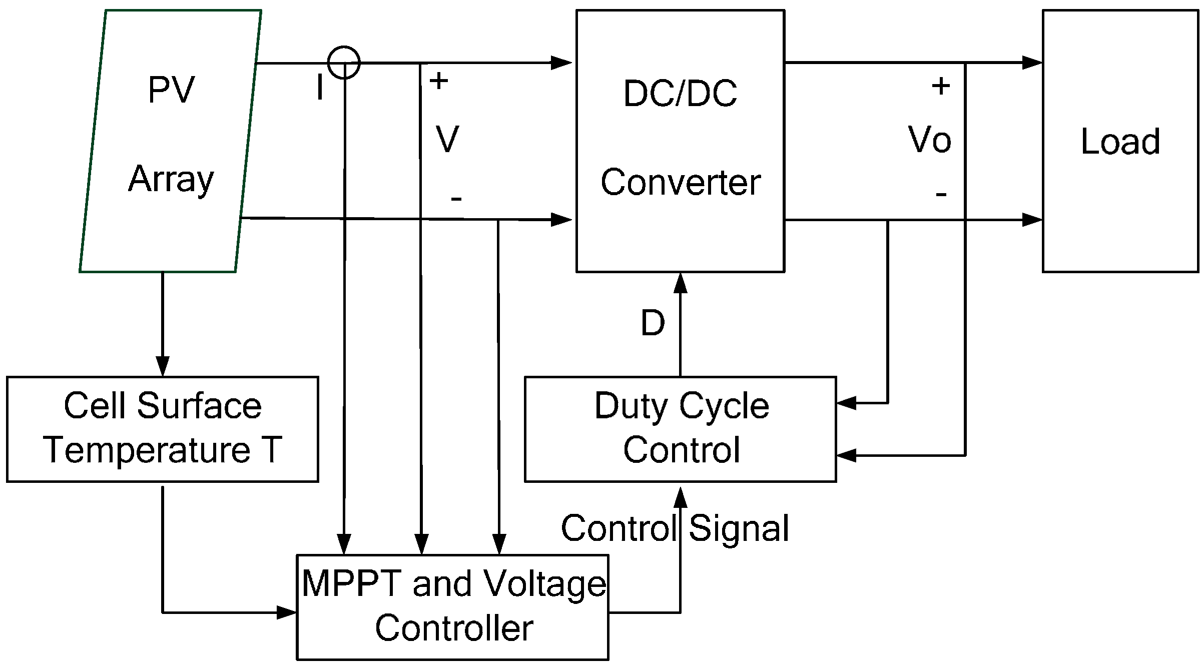
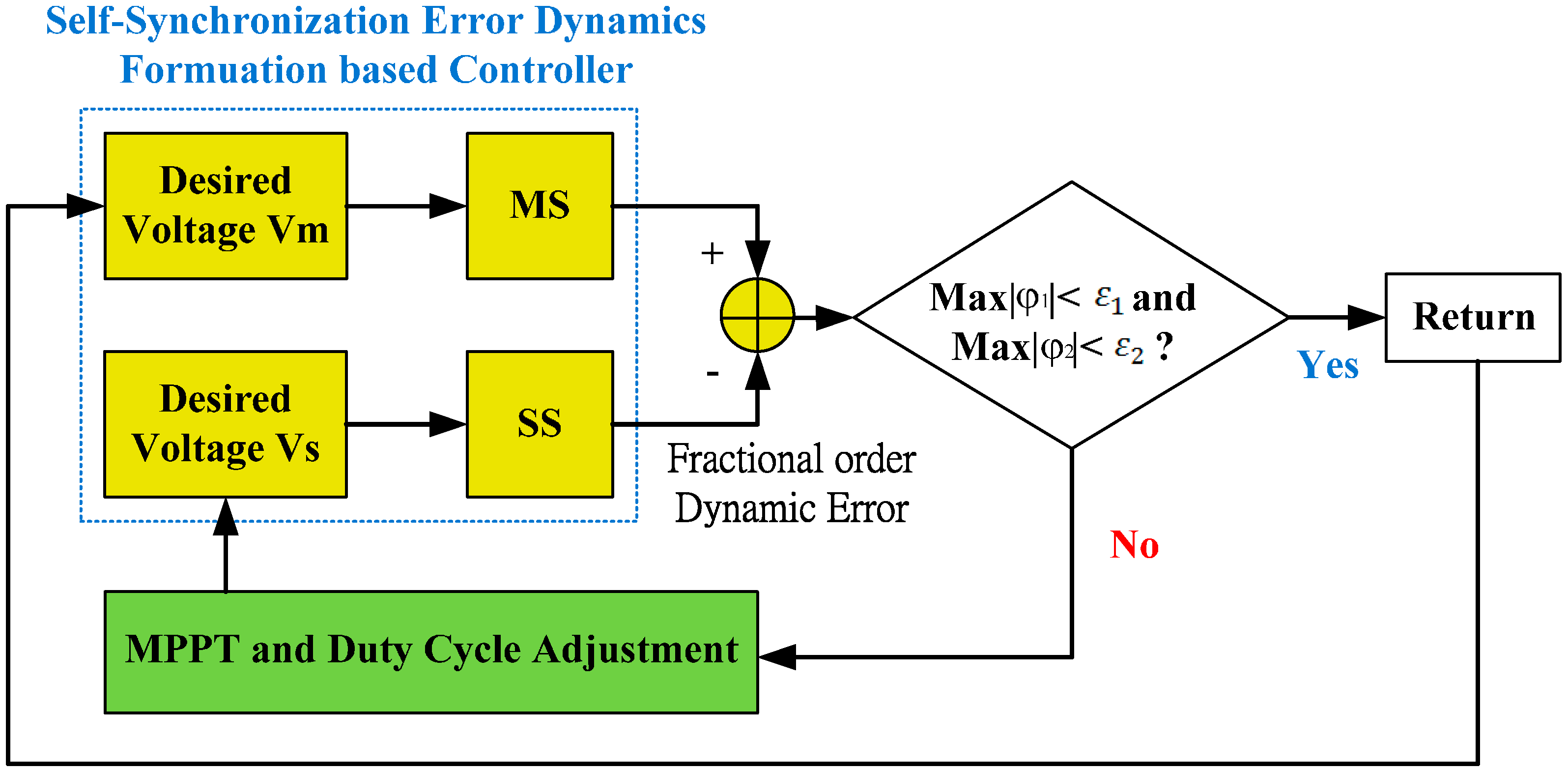
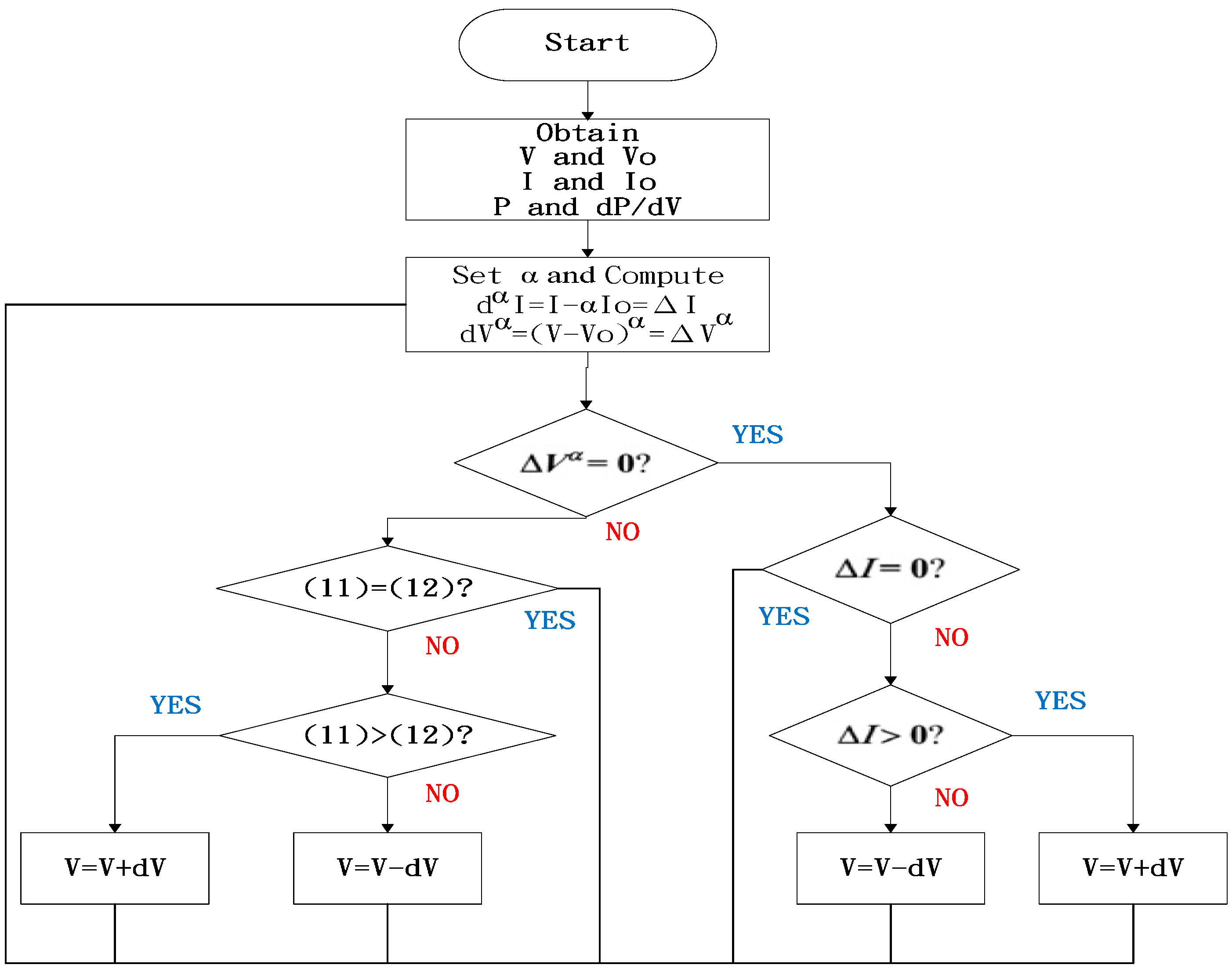
3. Design of Voltage Detector

This section will describe the design process of the voltage detector in detail. Table 1 presents the associated notation and definitions.

Table 1. Notation and definitions.

Notation	Definition
$X{m}_i$	The system states of master system
$X{s}_i$	The system states of slave system
$F_i$	Nonlinear functions
$E_i=X{m}_i-X{s}_i$	Error states of chaos synchronization system
x	System state of Sprott Chaos System
$\text{sign}(\text{Δ})$	Symbolic function is defined as $\text{sign}(\text{Δ})=\{\begin{array}{c}+1\text{, if Δ}\ge 0\\ -1\text{, if Δ}<0\end{array}$
a, b	System parameters of Sprott Chaos System
$e_i=X{m}_i-X{s}_i;i=1,2,3$	Error states of Sprott Chaos System
$\mathrm{\alpha }$	The value of fractional order
$t_0$	Initial time
$D_t$	Differential with respect to time t
$t\prime =\frac{1}{{(\text{Δ}t)}^{\text{α}}},a\prime =\frac{a}{{(\text{Δ}t)}^{\text{α}}},b\prime =\frac{b}{{(\text{Δ}t)}^{\text{α}}}$	System parameters of fractional order system
$\mathrm{\Delta }t$	Sampling time
$V_m$	The data of expected voltage
$V_s$	The data of real-time test voltage
${\text{φ}}_1$, ${\text{φ}}_2$	Dynamic error equation as the variables of error judgment of chaos synchronization dynamic error detector
${\text{ε}}_1$, ${\text{ε}}_2$	The set values of error magnitude

Table 1. Notation and definitions.

Notation	Definition
$X{m}_i$	The system states of master system
$X{s}_i$	The system states of slave system
$F_i$	Nonlinear functions
$E_i=X{m}_i-X{s}_i$	Error states of chaos synchronization system
x	System state of Sprott Chaos System
$\text{sign}(\text{Δ})$	Symbolic function is defined as $\text{sign}(\text{Δ})=\{\begin{array}{c}+1\text{, if Δ}\ge 0\\ -1\text{, if Δ}<0\end{array}$
a, b	System parameters of Sprott Chaos System
$e_i=X{m}_i-X{s}_i;i=1,2,3$	Error states of Sprott Chaos System
$\mathrm{\alpha }$	The value of fractional order
$t_0$	Initial time
$D_t$	Differential with respect to time t
$t\prime =\frac{1}{{(\text{Δ}t)}^{\text{α}}},a\prime =\frac{a}{{(\text{Δ}t)}^{\text{α}}},b\prime =\frac{b}{{(\text{Δ}t)}^{\text{α}}}$	System parameters of fractional order system
$\mathrm{\Delta }t$	Sampling time
$V_m$	The data of expected voltage
$V_s$	The data of real-time test voltage
${\text{φ}}_1$, ${\text{φ}}_2$	Dynamic error equation as the variables of error judgment of chaos synchronization dynamic error detector
${\text{ε}}_1$, ${\text{ε}}_2$	The set values of error magnitude

3.1. Chaos Theory and Chaos Synchronization Dynamic Error

Chaos theory [16,17] is a nonlinear system theory. It is characterized by unpredictability and irregular motion. The chaos system makes dramatic change in micro variation. The chaos synchronization synchronizes the kinematic trajectories of two chaos systems, and the controller makes the error zero [18,19]. In the chaos synchronization system, the two chaos systems are called Master System (MS) and Slave System (SS). When the two systems have different initial values, the kinematic trajectories of the two systems have different chaos phenomena. However, when a controller is added to the SS to track the MS, and the MS and SS act in synchronization, the kinematic trajectories of two chaos systems have the same change at the same time. The MS and SS are defined as follows:

$$MS=\{\begin{array}{c}\dot{X}X{m}_1(t)=F_1(t,[X{m}_1,X{m}_2\cdots X{m}_n])\\ \dot{X}{m}_2(t)=F_2(t,[X{m}_1,X{m}_2\cdots X{m}_n])\\ \dot{X}{m}_n(t)=F_n(t,[X{m}_1,X{m}_2\cdots X{m}_n])\end{array}$$

(4)

$$SS=\{\begin{array}{c}\dot{X}{s}_1(t)=F_1(t,[X{s}_1,X{s}_2\cdots X{s}_n])\\ \dot{X}{s}_2(t)=F_2(t,[X{s}_1,X{s}_2\cdots X{s}_n])\\ \dot{X}{s}_n(t)=F_n(t,[X{s}_1,X{s}_2\cdots X{s}_n])\end{array}$$

(5)

The characteristic quantity extracted in this paper is the naturally tracked dynamic error amount of MS and SS in the master-slave synchronization system. Therefore, there is no controller for the master-slave synchronization system in this paper; as long as the master and slave chaos systems are subtracted from each other, the dynamic error status can be obtained.

$$E=MS-SS=\{\begin{array}{c}{\dot{E}}_1(t)=F_1(t,[E_1,E_2\cdots E_n])\\ {\dot{E}}_2(t)=F_2(t,[E_1,E_2\cdots E_n])\\ ⋮\\ {\dot{E}}_n(t)=F_n(t,[E_1,E_2\cdots E_n])\end{array}$$

(6)

where $E_1=X{m}_1-X{s}_1$, $E_2=X{m}_2-X{s}_2$, $E_n=X{m}_n-X{s}_n$, the final dynamic error status has chaos phenomenon, and the controller makes a decision based on a dynamic analysis of the error status.

3.2. Fractional Order Chaos Synchronization Dynamic Error

In terms of signal processing, the chaos synchronization system is often used to check the power quality, voltage oscillation, and control application [20,21]. The dynamic behavior can make an abnormal signal track normal signal. In order to implement the synchronization of master signal (MS) and slave signal (SS), the SS uses the MS signal as a reference signal. In reference [19], Kuo et al. focused on the tracking time and the number of tracking cycle on MPPT. However, their study did not discuss the steady-state responses. In this study, we will use the same concept to discuss the steady-state behaviors of MPPT in this study. This paper also uses the Sprott Chaos System [22] to discuss it. The equation for the Sprott chaos system is:

$$\stackrel{⃛}{x}+a\ddot{x}+b\dot{x}=-1.2x+2\text{sign}(x)$$

(7)

where the symbolic function (Δ) is defined as:

$$\text{sign}(\text{Δ})=\{\begin{array}{c}+1\text{, if Δ}\ge 0\\ -1\text{, if Δ}<0\end{array}$$

(8)

The dynamic equation of MS and SS in Sprott Chaos System can be defined as:

$$\{\begin{array}{c}{\dot{X}}_{m_1}=X_{m_2}\\ {\dot{X}}_{m_2}=X_{m_3}\\ {\dot{X}}_{m_3}=-a{X}_{m_3}-b{X}_{m_2}-1.2X_{m_1}+2\text{sign}(X_{m_1})\end{array}$$

(9)

$$I_{ph}=[I_{sc}+k_{sc}(T-T_r)]\frac{S}{1000}$$

(10)

In the state of dynamic error, the error variance is defined as $e_1=X{m}_1-X{s}_1$, $e_2=X{m}_2-X{s}_2$, $e_3=X{m}_3-X{s}_3$, and $e={\left[e_1,e_2,e_3\right]}^T$. Equations (9) and (10) are changed to a matrix pattern:

$$\left[\begin{array}{c}{\dot{e}}_1\\ {\dot{e}}_2\\ {\dot{e}}_3\end{array}\right]=\left[\begin{array}{ccc}0& 1& 0\\ 0& 0& 1\\ -1.2& -b& -a\end{array}\right]e+2\left[\begin{array}{c}0\\ 0\\ \text{sign}(X{m}_1)-\text{sign}(X{s}_1)\end{array}\right]$$

(11)

The system state variables $X{m}_1$ and $X{s}_1$ capture the sinusoid in positive period or negative period synchronization, so $\text{sign}(X{m}_1)-\text{sign}(X{s}_1)=0$, according to Kuo et al. [19], the system in Equation (11) can be reduced to the following second-order system:

$$\left[\begin{array}{c}{\dot{e}}_2\\ {\dot{e}}_3\end{array}\right]=\left[\begin{array}{cc}0& 1\\ -b& -a\end{array}\right]\left[\begin{array}{c}{e}_2\\ e_3\end{array}\right]=\left[A\right]\tilde{e}$$

(12)

As $a>0$ and $b>0$, Equation (12) is tenable. The fractional order general expression in [12] is used in this chaos system; the fractional order general expression can be expressed as:

$$\frac{{\text{d}}^{\text{α}}e(t)}{\text{d}{t}^{\text{α}}}\approx \underset{\text{Δ}t\to 0}{\lim }\frac{e(t)-\text{α}e(t-t_0)}{{(t-(t-t_0))}^{\text{α}}}\approx \frac{e(t)-\text{α}e(t-t_0)}{{(\text{Δ}t)}^{\text{α}}}$$

(13)

when α = 1, the α value is 0–1 in fractional order. The fractional order geometric interpretation of Equation (13) has been described [21].

Equation (12) can be expressed in fractional order:

$$\left[\begin{array}{c}{D_t}^{\text{α}}{e}_2\\ {D_t}^{\text{α}}{e}_3\end{array}\right]\approx \left[\begin{array}{cc}0& t\prime \\ -b\prime & -a\prime \end{array}\right]\left[\begin{array}{c}{e}_2(t)\\ e_3(t)\end{array}\right]+\left[\begin{array}{cc}0& -\text{α}t\prime \\ -\text{α}b\prime & -\text{α}a\prime \end{array}\right]\left[\begin{array}{c}{e}_2(t-t_0)\\ e_3(t-t_0)\end{array}\right].$$

(14)

If t₀ is the initial time, the system parameter is changed to:

$$t\prime =\frac{1}{{(\mathrm{\Delta }t)}^{\text{α}}},a\prime =\frac{a}{{(\mathrm{\Delta }t)}^{\text{α}}},b\prime =\frac{b}{{(\mathrm{\Delta }t)}^{\text{α}}}$$

(15)

where $0<\text{α}<1$ is the fractional order. This fractional order dynamic error equation is used in the PV panel end to capture the different dynamic behaviors of transient voltage as the signal ends. Therefore, we define variables $x{m}_2=V_m[i]$, $x{m}_3=V_m[i+1]$, and $i\in [1,n-1]$; these are the data for expected voltage $V_m$ extracted from the signal end. $x{s}_2=V_s[i]$, $x{s}_3=V_s[i+1]$ provide the data for real-time test voltage $V_s$ extracted from the signal end. The two signals are used as criteria for real-time synchronization dynamic error detection.

In order to redefine and calculate ${D_t}^{\text{α}}{e}_2$ and ${D_t}^{\text{α}}{e}_3$ after fractional-order differentiation, Equation (14) is changed to the following equation:

$$\begin{array}{l}\left[\begin{array}{c}{\text{φ}}_1\\ {\text{φ}}_2\end{array}\right]\approx \left[\begin{array}{cc}0& t\prime \\ -b\prime & -a\prime \end{array}\right]\left[\begin{array}{c}{e}_2[i]\\ e_3[i]\end{array}\right]+\left[\begin{array}{cc}0& -\text{α}t\prime \\ -\text{α}b\prime & -\text{α}a\prime \end{array}\right]\left[\begin{array}{c}{e}_2[i-1]\\ e_3[i-1]\end{array}\right],\\ i\in [1,n-1]\end{array}$$

(16)

where error variance $e_2[i]=V_m[i]-V_s[i]$, $e_3[i]=V_m[i+1]-V_s[i+1]$, $e_2[i-1]=V_m[i-1]-V_s[i-1]$, $e_3[i-1]=V_m[i]-V_s[i]$, $V_m=V_s=0$ in initial state, and ${\text{φ}}_1$ and ${\text{φ}}_2$ are extracted from dynamic error equation as the variables of error judgment of chaos synchronization dynamic error detector.

3.3. Implementation of Voltage Detector

According to Figure 2, the cell temperature of PV panel rises gradually in the sunlight, the output power decreases as the cell temperature rises, and the output voltage decreases as the cell temperature rises. Because of this characteristic, at the first MPPT, the voltage V_m can be regarded as the MPP voltage. When the cell temperature changes, the PV curve of the PV panel shifts left, since the voltage from the PV panel is related to cell temperature. The following equation can be obtained:

$$V=\frac{n_{s}bTA}{q}\ln (\frac{n_p{I}_{ph}+n_p{I}_{sat}-I}{n_p{I}_{sat}})$$

(17)

$$V_m=V+\text{σ}(T_c-25),$$

(18)

where $T_c$ is the surface cell temperature of PV panel and $\text{σ}$ is the cell temperature compensation coefficient. The control mode of voltage detector is shown in Figure 4.

Figure 4. Schematic diagram of chaos synchronization dynamic error detector control.

Figure 4. Schematic diagram of chaos synchronization dynamic error detector control.

The operating method of the controller is shown in the above figure; when the dynamic errors ${\text{φ}}_1$ and ${\text{φ}}_2$ are smaller than the set ${\text{ε}}_1$ and ${\text{ε}}_2$ values, the error magnitude does not exceed the set value, meaning if the PV panel is working somewhere about the MPP, the MPPT is not executed. On the contrary, when the dynamic errors ${\text{φ}}_1$ and ${\text{φ}}_2$ are greater than the set ${\text{ε}}_1$ and ${\text{ε}}_2$ values, meaning the PV panel is not working around the MPP due to cell temperature change or other factors, the MPPT is restarted to track the MPP.

The flowchart of the fractional order incremental conductance method used in this paper is modified as Figure 5. This method uses voltage V and current I as inputs. The variation of voltage and current are approximated as $d^{\text{α}}I=I-\text{α}{I}_o$ and $d{V}^{\text{α}}={(V-V_o)}^{\text{α}}$.

This controller does not implement MPPT when the dynamic error is not large, so as to reduce the power oscillation loss by MPPT in steady state. The simulation and experimental results are shown in the next section.

Figure 5. Algorithm flowchart of FOICM.

Figure 5. Algorithm flowchart of FOICM.

4. Simulation and Experimental Results

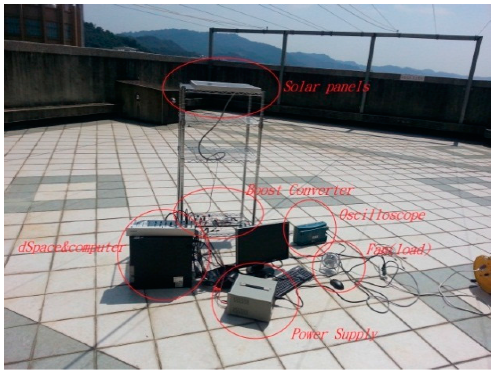
4.1. Simulation and Experimental Equipment

The main pieces of simulation and experimental equipment are a model and a controller of a PV power system built using a PC host as MATLAB R2012a Simulink (MathWork, New York, NY, USA). The host specifications are Intel core i7-3770 CPU 3.4 Ghz (Intel, New York, NY, USA) and 8 G memory (Intel, Santa Clara, CA, USA). The specifications of the PV panel are shown in Table 2; the maximum power is 17 W, the open-circuit voltage is 21.24 V, and the maximum operating point voltage is 16 V.

Table 2. Specific parameters of the proposed PV array (at solar radiation of 1 kW·m⁻² and a cell temperature of 25 °C).

Specific Parameter	Value
Maximum Power $P_{max}$	17 (W)
Maximum Power Voltage ($V_{mp}$)	16 (V)
Maximum Power Current ($I_{mp}$)	1.06 (A)
Open circuit Voltage ($V_{OC}$)	21.24 (V)
Short circuit Current ($I_{SC}$)	1.2 (A)
Operating Cell temperature Range	−40 °C–85 °C

Table 2. Specific parameters of the proposed PV array (at solar radiation of 1 kW·m⁻² and a cell temperature of 25 °C).

Specific Parameter	Value
Maximum Power $P_{max}$	17 (W)
Maximum Power Voltage ($V_{mp}$)	16 (V)
Maximum Power Current ($I_{mp}$)	1.06 (A)
Open circuit Voltage ($V_{OC}$)	21.24 (V)
Short circuit Current ($I_{SC}$)	1.2 (A)
Operating Cell temperature Range	−40 °C–85 °C

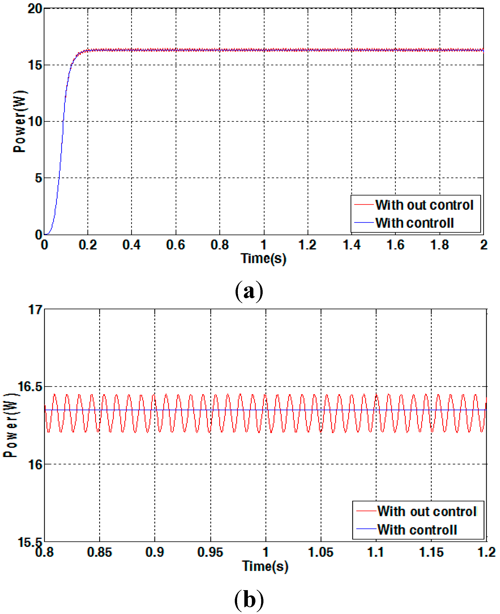
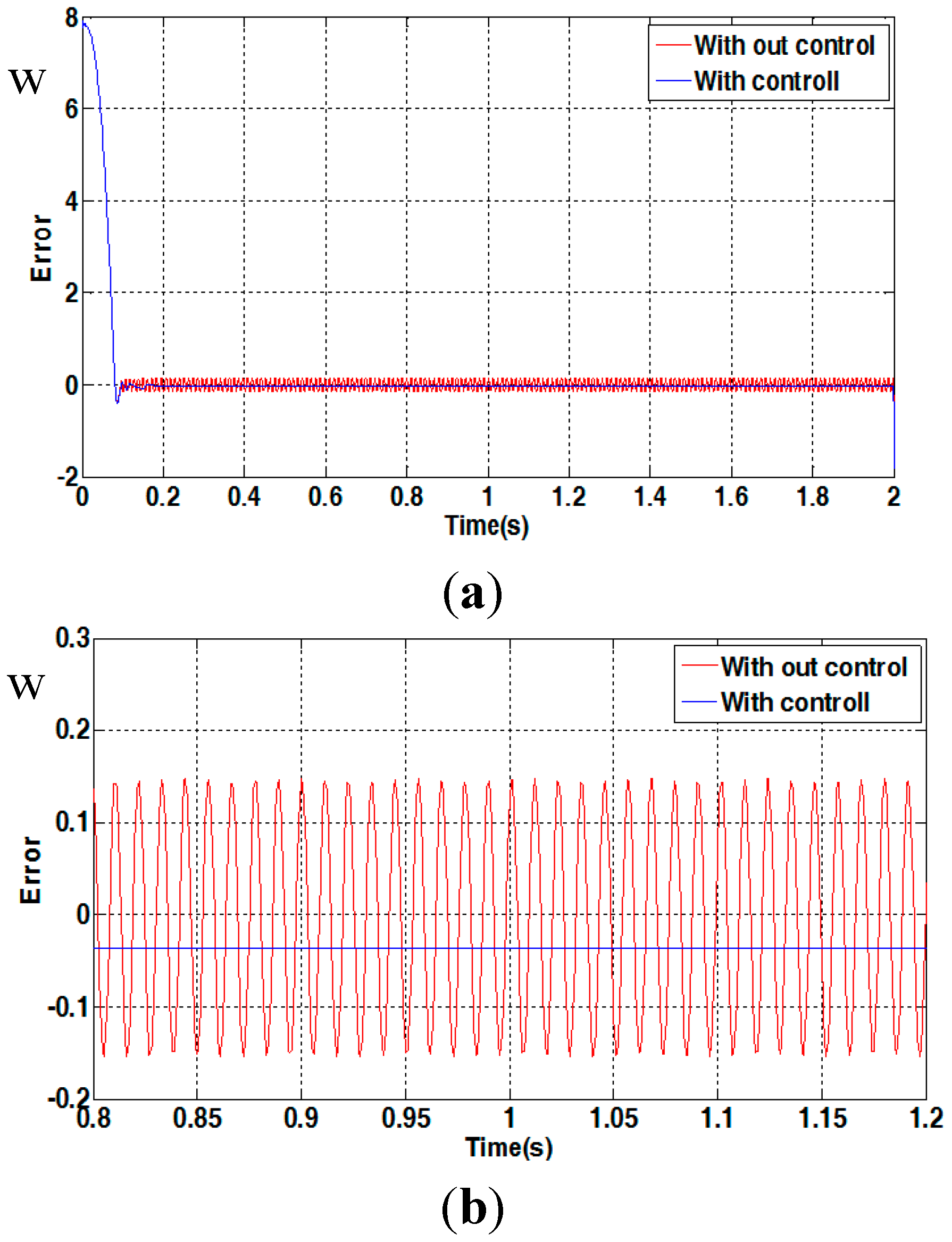
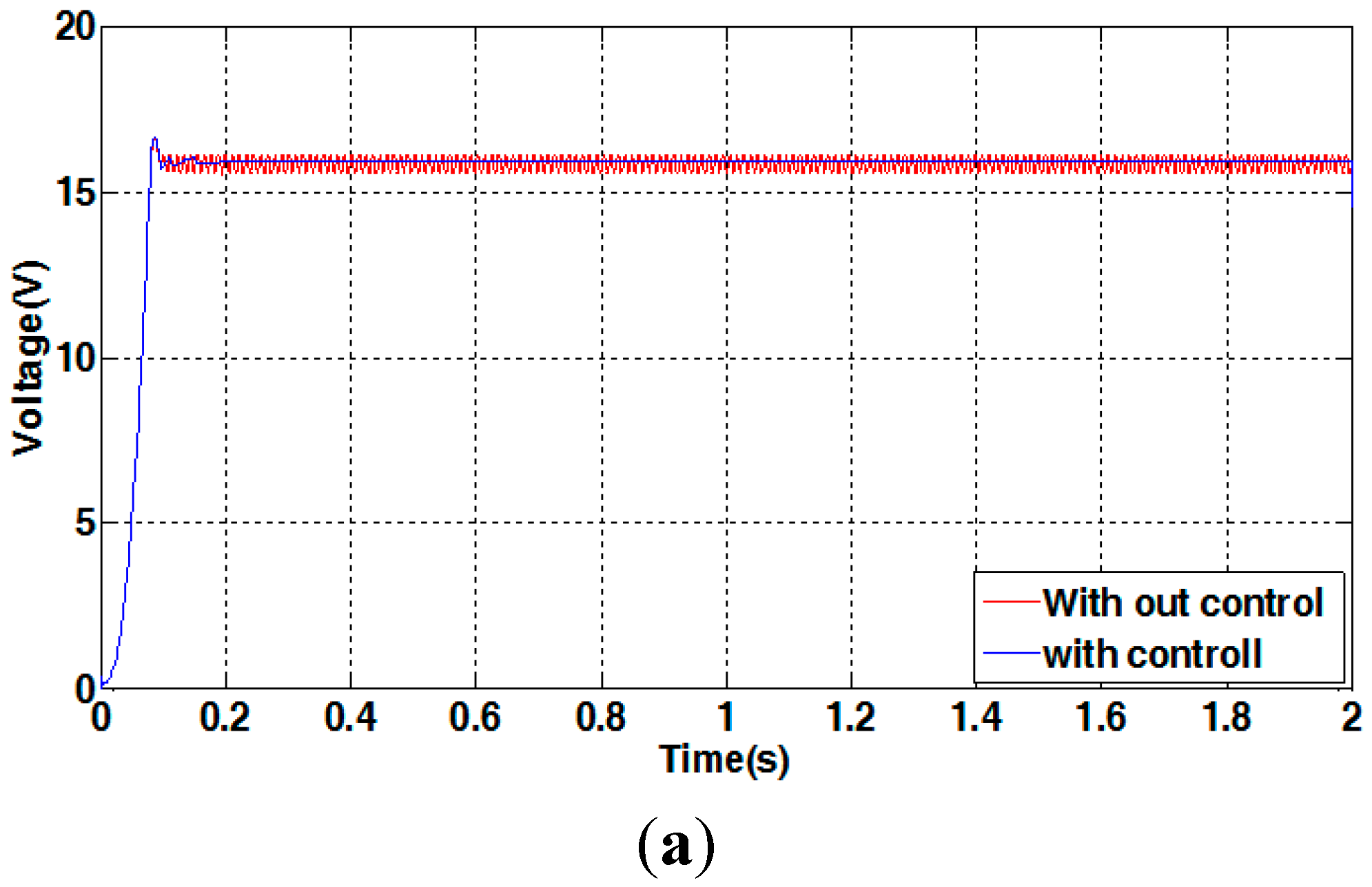
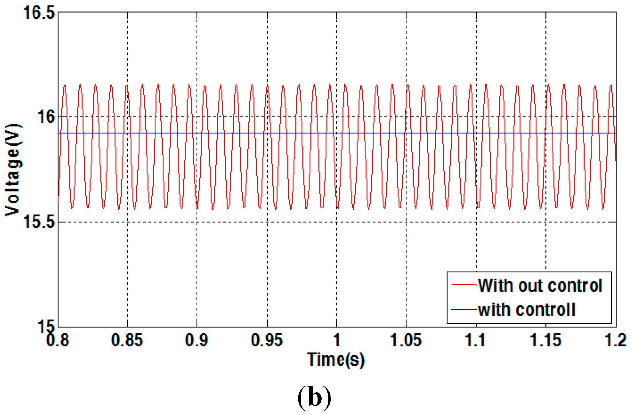
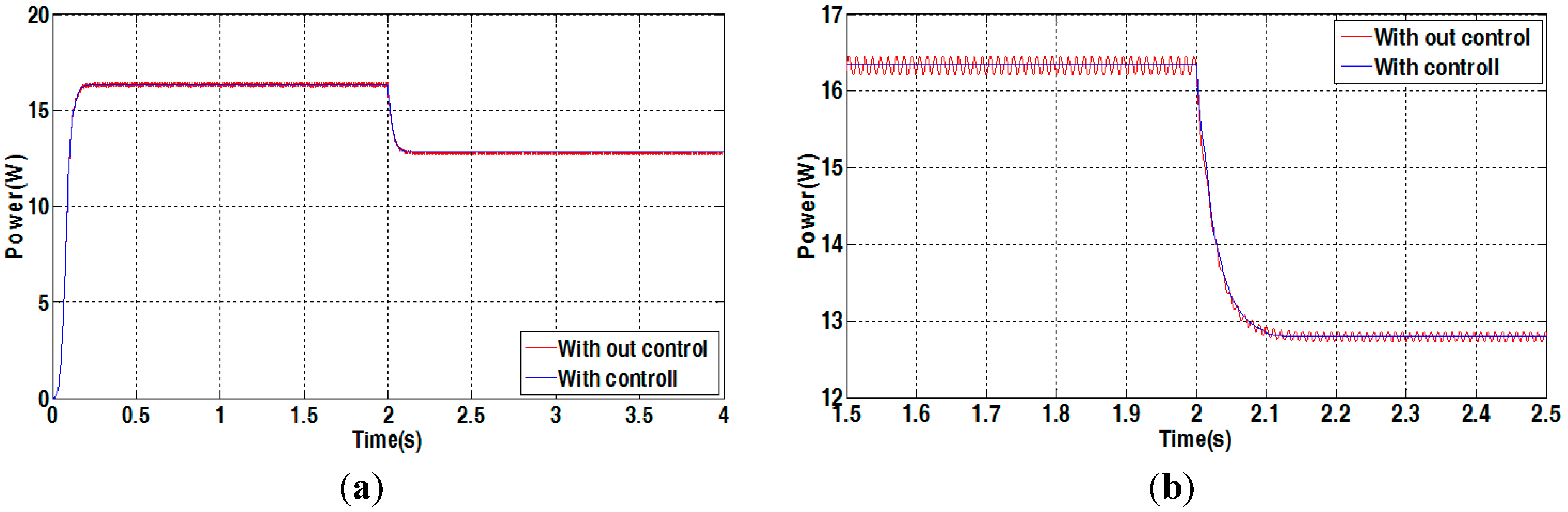
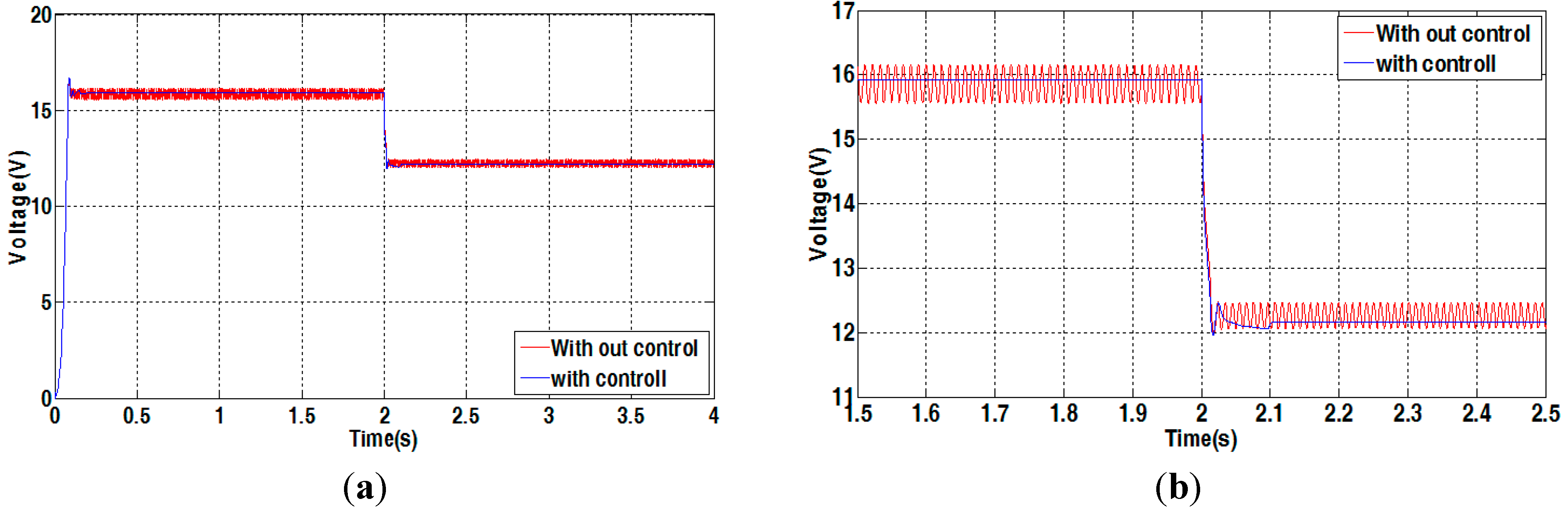
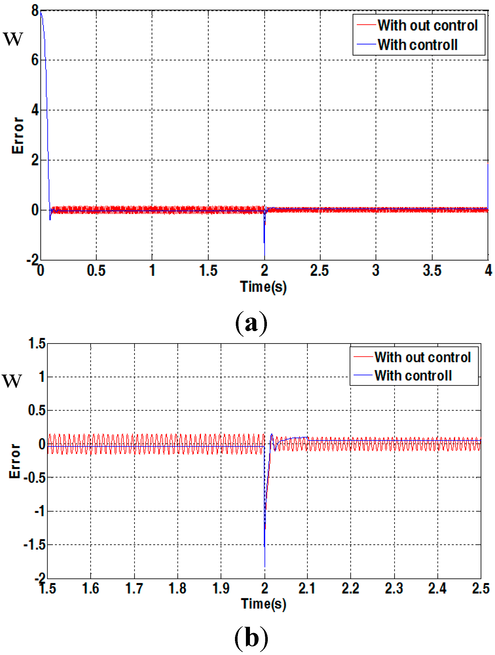
4.2. Simulation Results

The first simulation is at illumination 1000 W·m⁻² and cell temperature 25 °C. Another simulated condition is 1000 W·m⁻², and cell temperature rises from 25 °C to 65 °C, with/without chaos synchronization dynamic error detector. The value of fractional order is selected as α = 0.1 in this paper. The simulation results are shown in Figure 6 and Figure 7. Figure 6 shows the power simulation of voltage detector, Figure 7 shows the voltage simulation of voltage detector, and Figure 8 shows the ${\text{φ}}_1$ error of chaos synchronization dynamic error.

Figure 6. (a) Power simulation comparison diagram of voltage detector at constant cell temperature; (b) power simulation comparison diagram of voltage detector at constant cell temperature in the range of 0.8 s to 1.2 s.

Figure 6. (a) Power simulation comparison diagram of voltage detector at constant cell temperature; (b) power simulation comparison diagram of voltage detector at constant cell temperature in the range of 0.8 s to 1.2 s.

Figure 7. (a) Voltage simulation comparison diagram of voltage detector at constant cell temperature; (b) voltage simulation comparison diagram of voltage detector at constant cell temperature in the range of 0.8 s to 1.2 s.

Figure 7. (a) Voltage simulation comparison diagram of voltage detector at constant cell temperature; (b) voltage simulation comparison diagram of voltage detector at constant cell temperature in the range of 0.8 s to 1.2 s.

Figure 8. (a) ${\text{φ}}_1$ simulation comparison diagram of voltage detector at constant cell temperature; (b) ${\text{φ}}_1$ simulation comparison diagram of voltage detector at constant cell temperature in the range of 0.8 s to 1.2 s.

Figure 8. (a) ${\text{φ}}_1$ simulation comparison diagram of voltage detector at constant cell temperature; (b) ${\text{φ}}_1$ simulation comparison diagram of voltage detector at constant cell temperature in the range of 0.8 s to 1.2 s.

Figure 6a and Figure 7a show that in the case without a voltage detector, as the MPPT continues all the while, the MPPT is still implemented in steady state, but the power and voltage are disturbed near the MPP, causing power loss. As shown in the enlarged view of Figure 6b and Figure 7b, the power and voltage oscillation is relatively small and almost stable under the control of a voltage detector. The variance in dynamic error value can be observed in Figure 8; as the voltage detector is used, the MPPT is stopped when the dynamic error is smaller than the set value, so the duty cycle is fixed. Therefore, the PV panel output will not continue oscillation for the variance in duty cycle, so as to reduce the power oscillation, and to reduce the power loss and prolong the lifetime of electronic modules.

The second simulated condition is 1000 W·m⁻² and the cell temperature rises from 25 °C to 65 °C. The cases with and without chaos synchronization dynamic error detector are compared.

Results for the simulation of power and voltage after cell temperature rise are shown in Figure 9 and Figure 10. Figure 11 shows the comparison results for dynamic error ${\text{φ}}_1$. The cell temperature changed from 25 °C to 65 °C at 2 s. It can be seen that the scheme also can track the MPP to within 0.1 s. It can also be seen that the steady-state oscillations will be suppressed when the control is active.

Figure 9. (a) Power simulation comparison diagram of voltage detector at variable cell temperature; (b) power simulation comparison diagram of voltage detector at variable cell temperature in the range of 1.5 s to 2.5 s.

Figure 9. (a) Power simulation comparison diagram of voltage detector at variable cell temperature; (b) power simulation comparison diagram of voltage detector at variable cell temperature in the range of 1.5 s to 2.5 s.

Figure 10. (a) Voltage simulation comparison diagram of voltage detector at variable cell temperature; (b) voltage simulation comparison diagram of voltage detector at variable cell temperature in the range of 1.5 s to 2.5 s.

Figure 10. (a) Voltage simulation comparison diagram of voltage detector at variable cell temperature; (b) voltage simulation comparison diagram of voltage detector at variable cell temperature in the range of 1.5 s to 2.5 s.

Figure 11. (a) ${\text{φ}}_1$ comparison diagram of voltage detector at variable cell temperature; (b) ${\text{φ}}_1$ comparison diagram of voltage detector at variable cell temperature in the range of 1.5 s to 2.5 s.

Figure 11. (a) ${\text{φ}}_1$ comparison diagram of voltage detector at variable cell temperature; (b) ${\text{φ}}_1$ comparison diagram of voltage detector at variable cell temperature in the range of 1.5 s to 2.5 s.

Figure 9 and Figure 10 show the power oscillation and loss caused by continuous MPPT in the case without a voltage detector. Figure 9b and Figure 10b show that the oscillation amplitude is reduced and almost stable under the control of a voltage detector. Figure 11 shows the real-time dynamic error detection. The MPPT is stopped when the error amount is smaller than the set value. It is obvious that the power and voltage oscillations are reduced. When the cell temperature changes at 2 s, the MPPT is implemented immediately as the error amount increases, and the MPPT is stopped when the maximum power is tracked. Thus, the PV panel supplies to the load at maximum power point, and the steady-state response is good. From the steady-state responses of MPPT, it can be seen that about 0.2 vibration amplitude can be suppressed with control action. Therefore, about 4% of the steady-state vibration energy can be saved. The system efficiency can be increased and the lifetime of electronic modules can be prolonged.

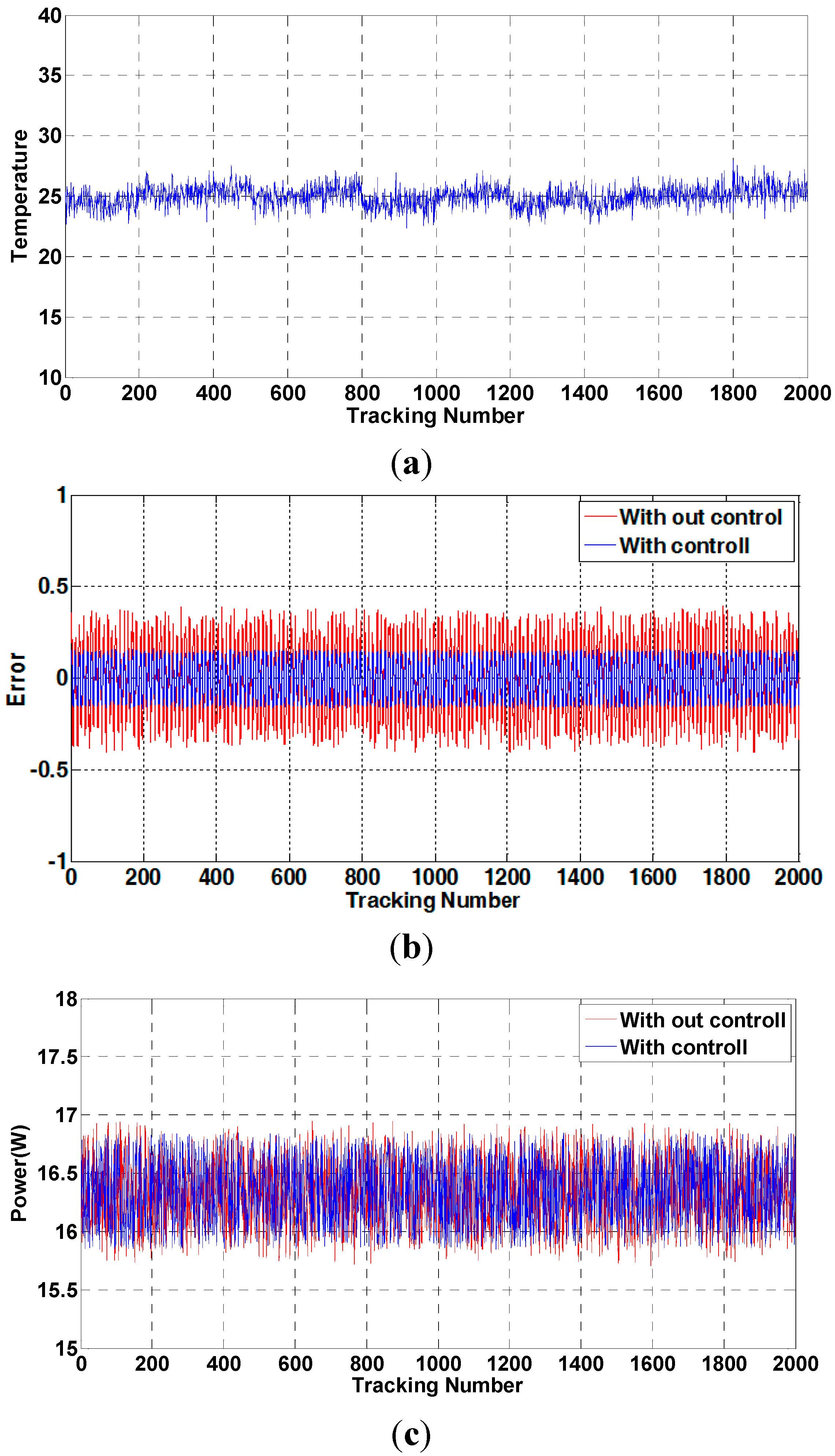
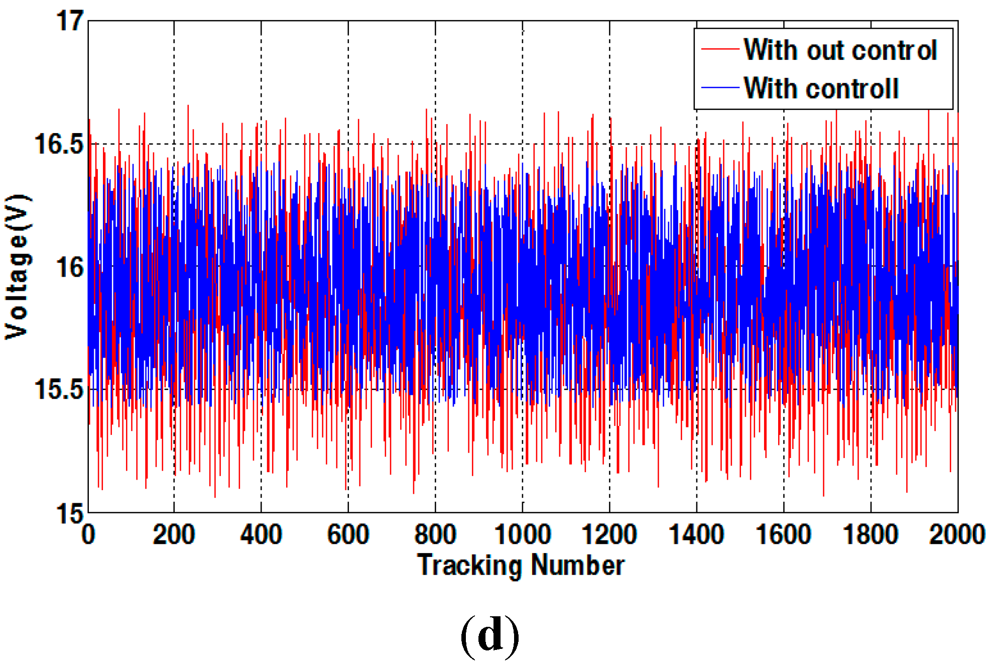
4.3. Experimental Results

The experimental equipment proposed in this paper is shown in Figure 12. The experiment was conducted at a normal cell temperature of 25 °C. The cell temperature is shown in Figure 13a; the experimental power, voltage, and dynamic error are shown in Figure 13b–d:

Figure 12. Experimental equipment.

Figure 12. Experimental equipment.

Figure 13. (a) Experimental cell temperature; (b) experimental power comparison diagram; (c) experimental voltage comparison diagram; (d) experimental φ₁ comparison diagram.

Figure 13. (a) Experimental cell temperature; (b) experimental power comparison diagram; (c) experimental voltage comparison diagram; (d) experimental φ₁ comparison diagram.

The selection of experimental equipment and sensing element may result in unnoticeable waveform variation in an experiment. The dynamic error φ₁ is also smaller than that without the voltage detector, meaning that the voltage oscillation amplitude is smaller. The voltage detector proposed in this paper further stabilizes the voltage of MPPT during steady-state response, so that the power loss is reduced effectively, the system efficiency is increased, and the service life of electronic modules is prolonged.

5. Conclusions

The fractional order chaos synchronization dynamic error detector used in this paper is applicable to any general MPPT methods. When a cell temperature sensing element and a voltage detector are added to the posterior pole, the other equipment does not need to be adjusted. This method improves the oscillation of a PV power system during steady-state response. According to the simulation results, the system still tracks the steady-state power at MPP, though as the cell temperature changes the voltage oscillation amplitude is reduced. The experimental results prove the feasibility and effectiveness of the fractional order chaos synchronization dynamic error detector proposed in this paper. From the steady-state responses of MPPT, it can be seen about 0.2 vibration amplitude can be suppressed with control action. Therefore, about 4% of the steady-state vibration energy can be saved. Therefore, the oscillation amplitude of voltage and power when the PV power system is in steady state is reduced, the power loss is reduced effectively, the system efficiency is increased, and the service life of electronic modules can be prolonged.

References

1. Di Silvestre, M.L.; Graditi, G.; Riva, S.E. A generalized framework for optimal sizing of Distributed Energy Resources in micro-grids using an Indicator-Based Swarm Approach. IEEE Trans. Ind. Inf. 2014, 10, 152–162. [Google Scholar] [CrossRef]
2. Kadri, R.; Gaubert, J.P.; Champenois, G. An Improved Maximum Power Point Tracking for Photovoltaic Grid-Connected Inverter Based on Voltage-Oriented Control. IEEE Trans. Ind. Electron. 2010, 58, 66–75. [Google Scholar] [CrossRef]
3. Bendib, B.; Belmili, H.; Krim, F. A survey of the most used MPPT methods: Conventional and advanced algorithms applied for photovoltaic systems. Renew. Sustain. Energy Rev. 2015, 45, 637–648. [Google Scholar] [CrossRef]
4. Salas, V.; Olías, E.; Barrado, A.; Lázaro, A. Review of the maximum power point tracking algorithms for stand-alone photovoltaic systems. Sol. Energy Mater. Sol. Cells 2006, 90, 1555–1578. [Google Scholar] [CrossRef]
5. Abdullah, M.A.; Yatim, A.H.M.; Tan, C.W.; Saidur, R. A review of maximum power point tracking algorithms for wind energy systems. Renew. Sustain. Energy Rev. 2012, 16, 3220–3227. [Google Scholar] [CrossRef]
6. Aurilio, G.; Balato, M.; Graditi, G.; Landi, C.; Luiso, M.; Vitelli, M. Fast Hybrid MPPT Technique for Photovoltaic Applications: Numerical and Experimental validation. Adv. Power Electron. 2014. [Google Scholar] [CrossRef]
7. Yu, K.N.; Liao, C.H.; Yau, H.T. A New Fractional-Order Based Intelligent Maximum Power Point Tracking Control Algorithm for Photovoltaic Power Systems. Int. J. Photoenergy 2015. [Google Scholar] [CrossRef]
8. Zheng, S.C.; Wang, L.Y. Research on Charging Control for Battery in Photovoltaic System. In Proceedings of the 6th IEEE Conference on Industrial Electronics and Applications (ICIEA), Beijing, China, 21–23 June 2011; pp. 2321–2325.
9. Elgammal, A.A.A.; Sharaf, A.M. Self-regulating particle swarm optimised controller for (photovoltaic-fuel cell) battery charging of hybrid electric vehicles. IET Electr. Syst. Trans. 2012, 2, 77–89. [Google Scholar] [CrossRef]
10. Gu, B.; Dominic, J.; Lai, J.S.; Zhao, Z.; Liu, C. High Boost Ratio Hybrid Transformer DC-DC Converter for Photovoltaic Module Applications. In Proceedings of the 27th Annual IEEE Applied Power Electronics Conference and Exposition (APEC), Orlando, FL, USA, 5–9 February 2012; pp. 2048–2058.
11. Li, H.; Monti, A.; Ponci, F.; D’Antona, G. Voltage Sensor Validation for Decentralized Power System Monitor Using Polynomial Chaos Theory. In Proceedings of the Instrumentation and Measurement Technology Conference (I2MTC), Austin, TX, USA, 3–6 May 2010; pp. 1633–1643.
12. Adinolfi, G.; Graditi, G.; Siano, P.; Piccolo, A. Multi-Objective Optimal Design of Photovoltaic Synchronous Boost Converters Assessing Efficiency, Reliability and Cost Savings. IEEE Trans. Ind. Inf. 2015, 11, 1038–1048. [Google Scholar] [CrossRef]
13. Graditi, G.; Adinolfi, G.; Tina, G.M. Photovoltaic optimizer boost converters: Temperature influence and electro-thermal design. Appl. Energy 2014, 115, 140–150. [Google Scholar] [CrossRef]
14. Graditi, G.; Adinolfi, G.; Femia, N.; Vitelli, M. Comparative Analysis of Synchronous Rectification Boost and Diode Rectification Boost Converter for DMPPT Applications. In Proceedings of the IEEE International Symposium on Industrial Electronics (ISIE 2011), Gdansk, Poland, 27–30 June 2011; pp. 1000–1005.
15. Graditi, G.; Adinolfi, G. Energy performances and reliability evaluation of an optimized DMPPT boost converter. In Proceedings of International Conference on Clean Electrical Power (ICCEP 2011), Ischia, Italy, 14–16 June 2011; pp. 69–72.
16. Monti, A.; Ponci, F. Uncertainty Evaluation Under Dynamic Conditions Using Polynomial Chaos Theory. IEEE Trans. Instrum. Meas. 2010, 59, 2825–2833. [Google Scholar] [CrossRef]
17. Leung, J.Y.-T.; Zhao, H. Minimizing Sum of Completion Times and Makespan in Master-Slave Systems. IEEE Trans. Comput. 2006, 55, 985–999. [Google Scholar] [CrossRef]
18. Suykens, J.A.K.; Curran, P.F.; Chua, L.O. Robust synthesis for master-slave synchronization of Lur’e systems. IEEE Trans. Circuits Syst. I Fundam. Theory Appl. 1999, 46, 846–850. [Google Scholar] [CrossRef]
19. Kuo, C.L.; Lin, C.H.; Yau, H.T.; Chen, J.L. Using Self-Synchronization Error Dynamics Formulation Based Controller for Maximum Photovoltaic Power Tracking in Micro-Grid Systems. IEEE J. Emerg. Sel. Top. Circuits Syst. 2013, 3, 459–467. [Google Scholar] [CrossRef]
20. Chen, S.J.; Zhan, T.S.; Huang, C.H.; Chen, J.L.; Lin, C.H. Nontechnical Loss and Outage Detection Using Fractional-Order Self-Synchronization Error-Based Fuzzy Petri Nets in Micro-Distribution Systems. IEEE Trans. Smart Grid 2014, 6, 411–420. [Google Scholar] [CrossRef]
21. Lin, C.H.; Chen, S.J.; Chen, J.L.; Kuo, C.L. Using Sprott Chaos Synchronization-Based Voltage Relays for Protection of Micro distribution Systems Against Faults. IEEE Trans. Power Deliv. 2013, 28, 2092–2102. [Google Scholar] [CrossRef]
22. Wu, X.J.; Lin, C.H.; Du, Y.C.; Chen, T. Sprott chaos synchronisation classifier for diabetic foot peripheral vascular occlusive disease estimation. IET Sci. Meas. Technol. 2012, 6, 533–540. [Google Scholar] [CrossRef]