A Computational Framework for Electric Scooter Neck Design Using Non-Uniform Rational B-Spline-Based Geometric Reconstruction of Topology-Optimized Structures

Abstract

This study presents a hybrid Non-Uniform Rational B-Spline (NURBS) methodology for the geometric reconstruction of topology-optimized structural components. NURBS are employed exclusively as a post-processing tool; all structural analyses are performed using standard finite elements (SOLID187 elements, ANSYS Mechanical R19.2), and isogeometric analysis (IGA) is not used. The methodology is validated on an Al 6061-T6 electric scooter neck under a 600 N static load. Two SIMP optimization iterations followed by a hybrid NURBS reconstruction reduce the component mass from 1.247 kg to 0.531 kg, achieving a 57.4% mass reduction. Finite element re-validation of the reconstructed geometry yields a maximum von Mises stress of 126.45 MPa (safety factor, SF = 2.18, exceeding the 2.0 requirement), a maximum deflection of 2.31 mm, and a first natural frequency of 127 Hz. Mesh convergence between the 2.5 mm and 1.25 mm refinements is Δ = 0.90%. Relative to the direct SIMP output (201 MPa), NURBS reconstruction reduces the peak stress by 37%, demonstrating that geometric post-processing is not a neutral step but a critical determinant of structural performance. Both fully automated STL reconstruction and edge-based NURBS reconstruction failed for this geometry class due to non-manifold topology and patch discontinuities, respectively. The proposed hybrid region-decomposition approach is the only method that has produced a watertight, FEA-compatible CAD model.

1. Introduction

Electric scooters have become increasingly prevalent in urban environments. With the recent rise in the popularity of electric scooters as a safe and environmentally friendly alternative to traditional motor vehicles, manufacturers are increasingly demanding components that are lightweight and structurally sound in real-life operating conditions. The neck is a significant part, as it links the handlebar stem with the front fork. It must be capable of dealing with both static and dynamic forces during riding, braking, and traversing obstacles, as well as satisfying minimum weight requirements [1,2].

Topology optimization has been established as the preferred method for determining optimal material distributions in structural components, most notably through the solid isotropic material with penalization (SIMP) approach [3,4,5]. The basic idea is simple: the algorithm takes into account the design area, loading conditions, and material conditions and identifies which structural elements can be eliminated safely without affecting the design integrity. Such an approach has been effectively used in the aerospace industry, the automotive industry, and the biomedical industry over the last 30 years, with a 30–60% reduction in mass without mechanical performance loss [6,7,8].

Nevertheless, there is a well-known limitation of topology optimization: the density field generated is difficult to integrate into a computer-aided design (CAD) environment. The final shape is usually exported as a triangulated STL (standard tessellation language) mesh. This is a separate, faceted representation that does not have the smooth surfaces that are needed for manufacturing operations and downstream finite element models. This raw data may need extensive post-processing to convert it into an accurate, editable CAD model [9,10].

Several reconstruction methods have been suggested to overcome this shortcoming. Considerable attention has been devoted to B-spline and NURBS-based techniques, which naturally produce smooth, parametric surfaces that can be translated to conventional CAD formats. Zhou [9] demonstrated that rotation-minimizing frame techniques can automatically convert 3D topology-optimized structures into high-quality, editable CAD models. These techniques are particularly effective when the geometry being rebuilt will be used in additive manufacturing, since the quality of the surface directly influences the ability to cope with the fatigue and precision of its dimensions.

More recently, researchers have started to use NURBS directly in the optimization framework instead of considering reconstruction as a distinct step. Giele et al. [10] suggested a component projection methodology which employs NURBS to make sure that the geometry is CAD-compatible throughout the entire optimization process. Urso et al. [11] extended this approach to design-dependent loading problems and showed that NURBS-based parameterization can be used to model complex physical scenarios with geometric integrity.

Another area of focus is automation. More recent efforts have proposed end-to-end pipelines that project the output of topology optimization to editable CAD models alone, based on the geometric decomposition and B-spline surface fitting [12]. These systems are reliable in moderate complexity geometries. However, the failure of fully automated processes in the construction of a real solid body is likely when dealing with optimized designs with branching topologies, thin walls, or non-manifold areas. This is the very problem that this paper will deal with.

The discipline is advancing rapidly. The integration of machine learning and generative design into NURBS-based workflows is creating new opportunities for automated geometry creation, as discussed in our previous examination of the future of NURBS in CAD [13]. The ramifications of these advancements indicate that the distinction between design optimization and geometric modeling will further blur in the coming years.

This paper investigates the direct resolution of the reconstruction bottleneck through fully automated STL reconstruction and edge-based NURBS reconstruction applied to the optimized scooter neck geometry; both methods ultimately failed due to non-manifold topology and patch discontinuities, respectively, resulting in a geometry that is not structurally valid. This led to a hybrid method: a semi-manual, region-decomposed NURBS reconstruction method that creates a watertight, smooth, and CAD-compatible geometry that can be re-validated by finite element methods.

The use of NURBS in this work needs clarification. NURBS are used purely as a geometric reconstruction tool in the mathematical frameworks of Gallier [14] and Piegl and Tiller [15]. They are not subjected to numerical analysis. Structural calculations are done using the standard finite element method (SOLID187 elements, ANSYS Mechanical R19.2). Isogeometric analysis (IGA) [16,17,18,19,20], which uses NURBS basis functions both as a geometry and analysis tool, is only mentioned to put the importance of NURBS in computational mechanics into perspective and not for the purpose of denoting the methodology used in the present paper.

The results clearly indicate that the conversion from the unrefined SIMP density field to the NURBS-reconstructed geometry diminishes the peak von Mises stress by 37%, decreasing it from 201 MPa to 126.45 MPa. The paper’s main contribution is a validated hybrid NURBS reconstruction pipeline that transforms a topology-optimized density field into a CAD geometry that is watertight and can be manufactured. This capability lies beyond the reach of traditional automated reconstruction approaches. The approach has been shown to lower the weight of an electric scooter neck made of Al 6061-T6 by 57.4%. It also has a safety factor of 2.18, a maximum deflection of 2.31 mm, and a first natural frequency of about 127 Hz. The remainder of this paper is organized as follows:

This work is motivated by a specific and documented failure: both automatic STL reconstruction and edge-based NURBS reconstruction were performed on the optimal neck shape, although neither produced a structurally valid result. It is impossible to compute a safety factor or validate a design without a working reconstruction. The hybrid methodology developed here is a direct engineering solution to this failure, as shown by the comparison results (

Table 1. A comparison of geometric reconstruction approaches for the SIMP-optimized electric scooter neck geometry.

Criterion	Automated STL	Edge-Based NURBS	Proposed Hybrid
Reconstruction result	FAILED—non-manifold topology	FAILED—patch discontinuities	SUCCESS ✓
Surface continuity	N/A	${\mathrm{C}}^0$ at patch boundaries	${\mathrm{C}}^1$ throughout
CAD compatibility (STEP)	N/A	Not achieved	STEP AP214 ✓
Min. wall thickness	N/A	Not enforced	2 mm enforced ✓
FEA re-validation	N/A	Not possible	${\sigma }_{VM}$ = 126.45 MPa ✓
Surface deviation (mm)	N/A	N/A—geometry invalid	<0.3 mm (CATIA deviation analysis)
Processing time (h)	~0.5 h (automated)	~2 h (semi-manual)	~3.5 h (hybrid)
Reproducibility	Not applicable	Not applicable	Documented 4-stage procedure (Section 3.4)

FAILED: the method did not produce a re-validatable geometry; SUCCESS: the method produced a watertight, FEA-validated geometry. ${\sigma }_{VM}$: von Mises stress.

) and the structural revalidation (SF: 1.37 → 2.18, peak stress −37%).

Section 2 provides a comprehensive evaluation of reconstruction methodologies, as well as the mathematical foundation of NURBS geometry and SIMP-based topology optimization.

Section 3 contains the case study, which includes setting up the FEA model, running SIMP optimization rounds, using a hybrid NURBS reconstruction method, and re-validating the final design structure.

Section 4 addresses the findings, the limitations, and further directions for research.

2. Mathematical Modeling of Geometries Using NURBS Basis Functions

2.1. CAD Reconstruction Using NURBS Geometric Representation

Non-Uniform Rational B-Splines (NURBS) constitute the prevailing geometric model employed in computer-aided design (CAD) tools, owing to their capacity to delineate free-form geometries and accurately represent precise analytic forms of curves, such as circles and conic sections. NURBS offer smoothness, compactness, and intrinsic compatibility with industrial CAD systems in structural design.

In the current study, NURBS are used exclusively as a geometric reconstruction tool, enabling the topology-optimization output to be converted into a smooth, manufacturable CAD model. No new NURBS formulations, numerical schemes, or algorithmic innovations are introduced. In turn, this section will be limited to a brief account of the NURBS representation that is relevant to the reconstruction process adopted.

A NURBS curve may be described as an aggregate of control points with a weighting to such an extent that $B_i\in$ $R_d$

$$C\left(\xi \right)={\sum }_{i=1}^n{R}_{i,p}\left(\xi \right)B_i$$

(1)

where the rational basis functions are given by:

$$R_{i,p}\left(\xi \right)={\displaystyle \frac{N_{i,p}\left(\xi \right)w_i}{W\left(\xi \right)}}={\displaystyle \frac{N_{i,p\left(\xi \right)w_i}}{{\sum }_{j=1}^n{N}_{j,p}\left(\xi \right)w_j}}$$

(2)

$N_{i,p}\left(\xi \right)$ are the B-spline basis functions of degree, $p,w_i$ are the associated positive weights, and $\xi$ denotes the parametric coordinate. When all weights are equal, the formulation reduces to the standard B-spline representation.

For surface modeling, a tensor product extension of the curve formulation is used. A NURBS surface is expressed as:

$$S\left(\xi ,\eta \right)=\sum _{i=0}^n\sum _{j=0}^m{R}_{i,j}^{p,q}(\xi ,\eta )P_{i,j}$$

(3)

where $P_{i,j}$ are the control points defining the bidirectional control net, and $R_{i,j}^{p,q}(\xi ,\eta )$ are the rational basis functions associated with the parametric directions ξ and η.

The geometry is loaded into CATIA V5 (Computer-Aided Three-dimensional Interactive Application, Dassault Systèmes), where NURBS surfaces are recreated with typical CAD tools [21]. The method yields seamless, continuous, and manufacturable geometry, validated by subsequent finite element analysis, emphasizing geometric accuracy over automated mesh-to-NURBS conversion. Standard references [14] provide extensive mathematical material regarding the theory of B-splines and NURBS.

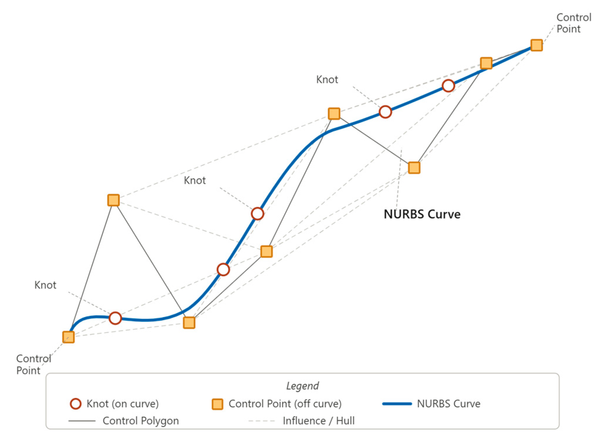
A NURBS curve is defined by a set of control points, a knot vector, and a set of weights that control the influence of each control point (Figure 1).

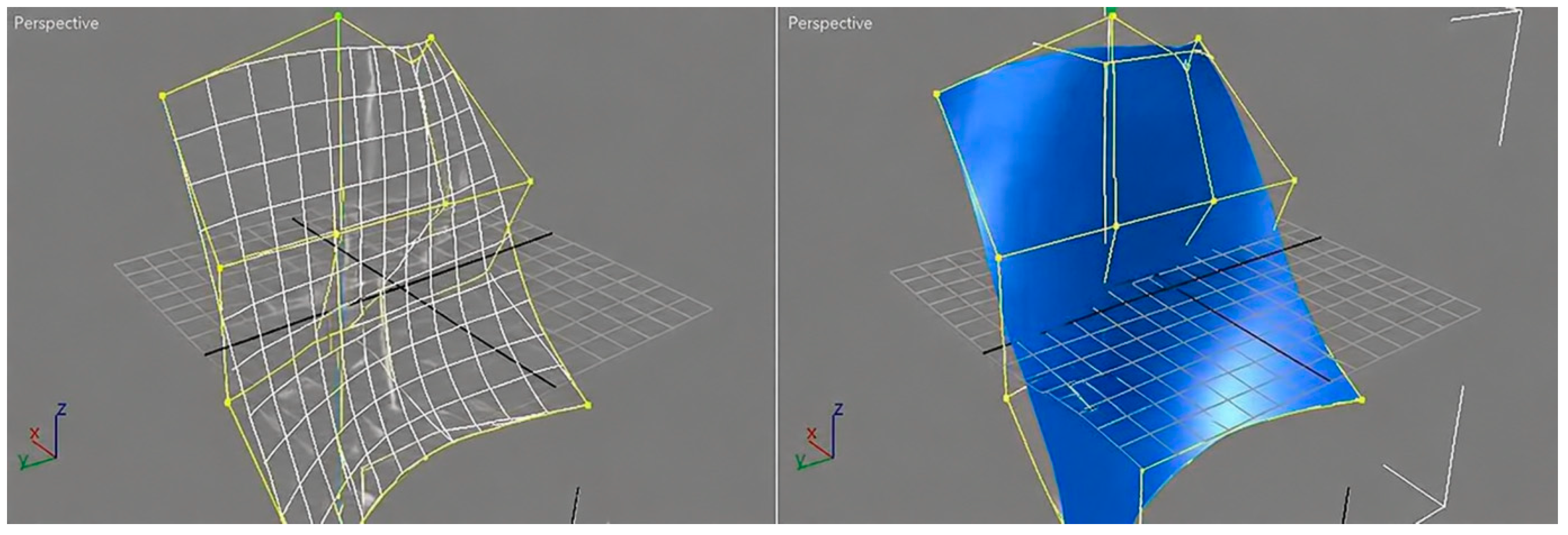
NURBS surfaces extend this formulation to a bi-parametric domain, enabling the representation of complex free-form surfaces (Figure 2).

2.2. Overview of Topology Optimization and Finite Element Analysis for Identifying and Eliminating Overloaded Zones

The most important method of determining the critically loaded areas of structural systems is the finite element method (FEM). This method breaks the continuous physical domains into discrete parts of some dimensions and transforms the equations of physical systems into solvable equations. The first equilibrium equation is given in Equation (4):

$$\left[K\right]\left\{u\right\}=\left\{F\right\}$$

(4)

In this context, [K] specifies the sum of the individual stiffness matrices of the included elements, u represents the nodal displacement vector, and F indicates the external force [3]. This equation has demonstrated utility in estimating displacements within the structure and, more critically, in evaluating the stress field, which identifies regions susceptible to material failure or stress limit violation.

The mesh discretization method is critical in the correct determination of overloaded regions since it plays a significant role in determining the accuracy and efficiency of the computation. Elements should be discretized with a thickness of 0.5 to 2 mm and aspect ratios of 3:1 or less to discretize joints and welds. Transition zones should comprise elements of 2 to 5 mm in thickness, and the low-stress areas can have components of 5 to 15 mm in thickness. To accurately capture the stress gradient in computational mechanics, at least 8 to 12 elements around the filet radii must be included in the mesh. The convergence study shows that the stresses obtained are not numerical artifacts, but physically significant quantities. The protocol requires at least three mesh refinements, and the element sizes should be in a ratio of about 1:4:16 and require the relative difference between the maximum stresses to be calculated using Equation (5):

$$\mathsf{\Delta }\sigma =|{\sigma }_{\mathrm{n}}-{\sigma }_{\mathrm{n}-1}|/{\sigma }_{\mathrm{n}}$$

(5)

Convergence was achieved when $\Delta \sigma$ was less than 1–2%. Sharp filet-free edges produce theoretically infinite stresses due to mathematical singularities; setting a minimum realistic filet radius of 0.5–1 mm removes these artifacts while maintaining a realistic manufacturing limit.

2.3. Solid Isotropic Material with Penalization (SIMP) Topology Optimization: Systematic Material Redistribution

Bendsoe developed the structural optimization method called solid isotropic material with penalization (SIMP). It treats optimal shape design as a material distribution problem. This method treats topology as a continuous material distribution, which makes it easier to optimize large design areas that discrete methods cannot evaluate well. Rozvany [5] showed that the SIMP methodology could effectively address complex issues utilizing finite elements and manage sophisticated design situations; nevertheless, its widespread implementation requires more time. Takezawa [6], in the Springer Handbook, notes that topology optimization is once again an important technology for additive manufacturing. It makes it feasible to directly link computational optima with final products that were previously limited by manufacturing constraints. This method uses a power-law interpolation methodology to connect the element density ρ (which ranges from 0 to 1) to the effective material stiffness, as shown in Equation (6).

$$E\left(\rho \right)=E_0·{\rho }^{\mathrm{p}}$$

(6)

where $p$ is the penalization exponent (typically $p=3$ for elastic problems). This power-law formulation penalizes intermediate densities and forces the optimization toward binary solutions (0 or 1), corresponding to either full material or void. The optimization problem is the minimization of the structural compliance, as in Equation (7):

$$C=F^{\mathrm{T}}u=u^{\mathrm{T}}Ku$$

(7)

(maximizing stability), and the volume constraint:

$$\mathsf{\Sigma }\left({\rho }_{\mathrm{i}}{\mathrm{V}}_{\mathrm{i}}\right)\le \mathrm{V}\mathrm{f}\mathrm{r}\mathrm{a}\mathrm{c}\mathrm{t}\mathrm{i}\mathrm{o}\mathrm{n}·\mathrm{V}\mathrm{t}\mathrm{o}\mathrm{t}\mathrm{a}\mathrm{l}$$

(8)

Equilibrium condition:

$$K\left(\rho \right)u=F$$

(9)

And density bounds:

$${\rho }_{\min }\le {\rho }_{\mathrm{i}}\le 1$$

(10)

where

$${\rho }_{\min }=0.001$$

(11)

It prevents numerical singularities. Papadopoulos [7] conducted a comprehensive numerical analysis demonstrating that for any isolated local or global minimizer of the infinite-dimensional problem, there exists a sequence of finite-element local minimizers that strongly converge to the minimizer in the pertinent space, thereby ensuring mathematical validity and confirming that the system of unfiltered discretized material distributions does not display checkerboarding artifacts under suitable regularizations.

The SIMP algorithm follows the cyclic steps of finite element analysis, sensitivity calculation, and density update. Each iteration was based on the solution of the FEA system.

$$K\left({\rho }^{\mathrm{k}}\right)u=F$$

(12)

Under all load cases, the compliance was yielded as follows:

$$C^{\mathrm{k}}=u^{\mathrm{T}}Ku$$

(13)

The computing sensitivities were as follows:

$$\partial C/\partial {\rho }_{\mathrm{i}}=-p·{{\rho }_{\mathrm{i}}}^{\mathrm{p}-1}·{u_{\mathrm{i}}}^{\mathrm{T}}{k}_0{u}_{\mathrm{i}}$$

(14)

Using the adjoint method, densities are optimized based on optimality criteria with a move limit of $m=0.2$, a damping coefficient of $\eta =0.5$, and filtering densities with the radius

$$r_{\min }=2-3\times elementsize$$

(15)

To avoid checkerboarding and guarantee mesh independence, the sensitivity is established as follows:

$$\partial C/\partial \rho$$

(16)

It is a measure of the contribution that each element makes to structural performance: large and negative values (material should be kept) and small and negative values (candidate for removal). The penalization exponent is in a continuation scheme such that $p=1$ during the first $20$ iterations of the scheme to permit intermediate densities to explore the design space, and then gradually rise to $p_{\max }=4$ to bring the solution to the binary. The convergence is obtained when

$$|C^{\mathrm{k}}-C^{\mathrm{k}-1}|/C^{\mathrm{k}}<0.001$$

(17)

Convergence is also declared when the relative change falls below 0.1% or when the maximum iteration count (150–200) is reached.

Checkerboarding in unfiltered solutions manifests as alternating solid-void structures that are numerically optimal yet physically insignificant. Density filtering enables a smooth change between the densities of the individual elements by using a weighted average between the densities of the individual and the surrounding elements to convert ill-posed optimization problems into well-posed problems with unique solutions. Zhu et al. [8] have shown that the moving morphable component (MMC) approach to SIMP in sequential topology optimization can be used to create multimodal multi-material structures that combine the benefits of explicit external structural topology with increased flexibility in internal multi-material structures, without sacrificing the simplicity of implementation. The density field ρ and the optimum density field ρ of each element are a quantitative measure of material efficiency: $\rho \approx 1$ (dense) means a material that is highly used and needs to be maintained or even strengthened.

$$0.3<\rho <0.9$$

(18)

This indicates the transition regions that need consideration, and $\rho \approx 0$(void) indicates that the material is under-utilized and can be removed or even reinforced. This density map provides a basis for systematic overload zone identification and material elimination procedures.

2.4. Methodology for Identifying and Eliminating Overloaded Zones

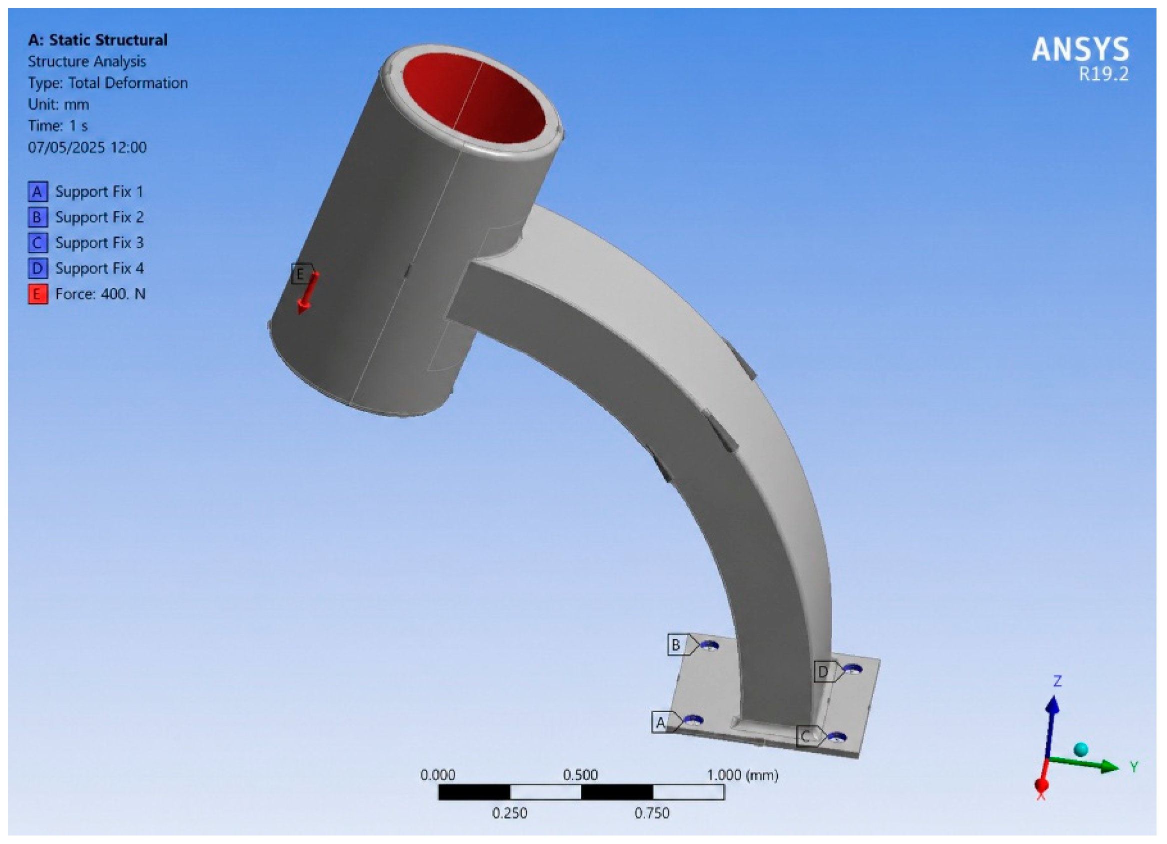
The research uses a single static vertical load of 600 N, which is about the same as the weight of a typical rider who weighs 80 kg while sitting in an urban area. This load was chosen as the representative dimensioning case because, consistent with the fork/steerer test load prescribed in ISO 4210-6 [22] and with the scooter structural analysis of Kim et al. [8], the nominal rider weight in the urban riding mode causes the highest sustained stress across all non-impact operating situations during the load envelope analysis. Impact loads (1500–3500 N during a 12 ms period) are temporary and affect fatigue rather than static yield assessment, which is the main structural criterion of the analysis. A thorough multi-load-case analysis is recognized as a constraint of the scope (see Section 4).

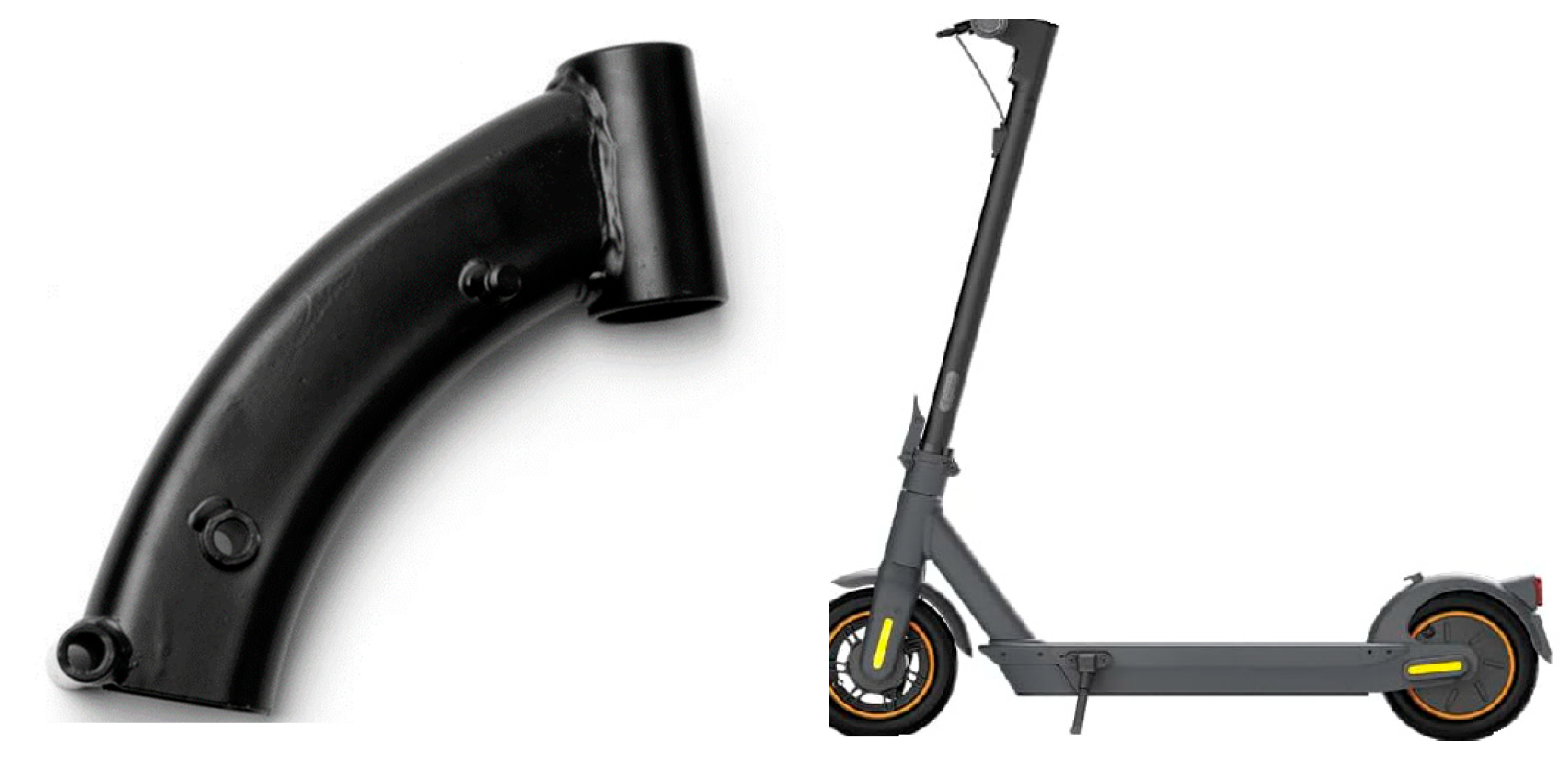
The focus is solely on optimization of the neck sub-component, depicted in Figure 3, which is an independent STEP file of the complete scooter assembly shown in Figure 4. No geometric simplifications were performed other than the removal of non-structural components (bearings, bolts, and handlebar clamp). The extracted geometry yields a base mass of 1.247 kg, calculated using the density of Al 6061-T6 (ρ = 2.7 × 10⁻⁶ kg/mm³) confirming geometric consistency between Figure 3 and Figure 4.

$${\mathit{\sigma }}_{\mathrm{vm},\max }\left(\mathit{i}\right)=\mathit{max}\left\{{\mathit{\sigma }}_{\mathrm{vm},1}\right(\mathit{i}),{\mathit{\sigma }}_{\mathrm{vm},2}(\mathit{i}),\dots ,{\mathit{\sigma }}_{\mathrm{vm},16}(\mathit{i}\left)\right\}$$

(19)

The multi-load-case analysis ensures that no critical loading scenario is overlooked, and the decisions of material removal are informed by the entire range of service cases.

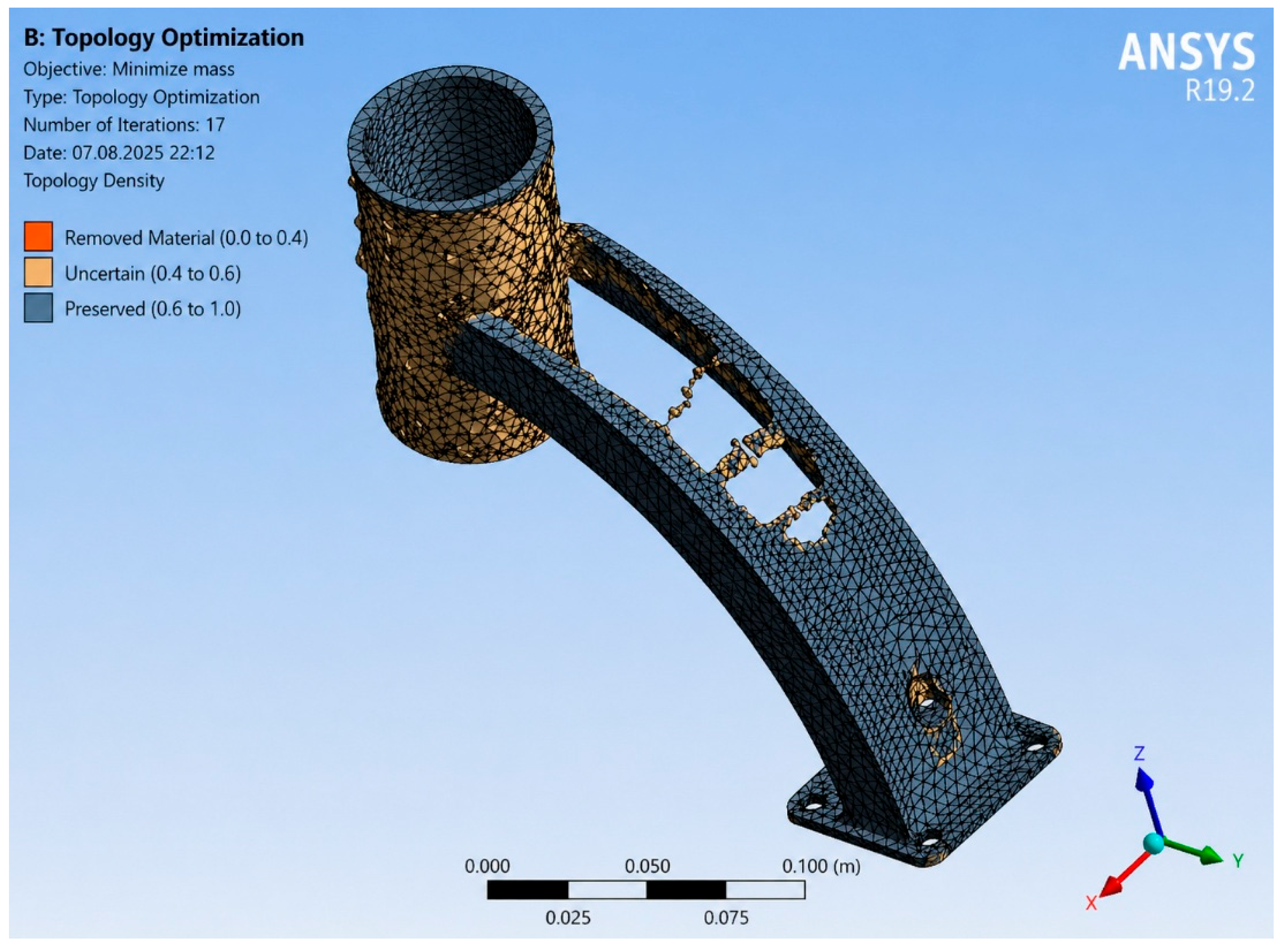
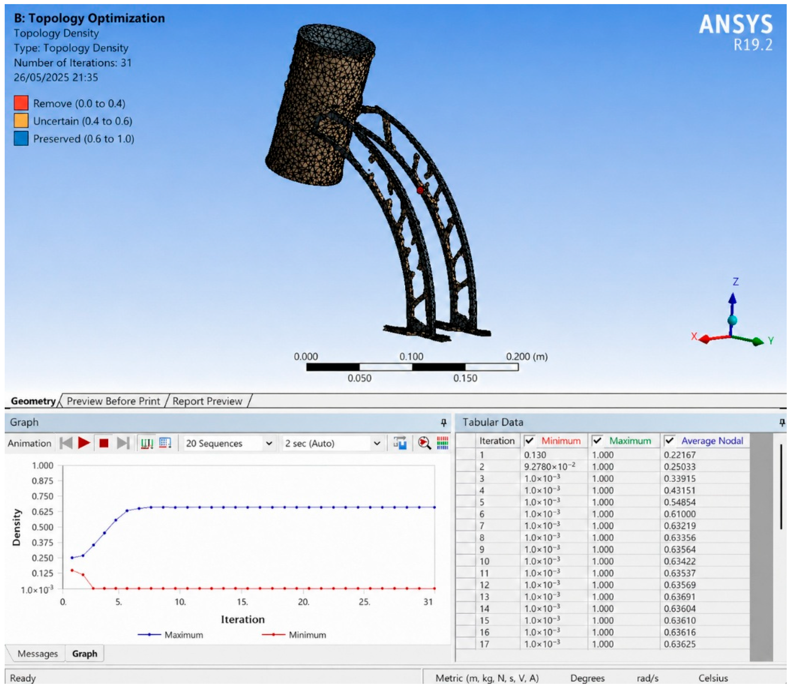
High-density regions with $\rho >0.9$ occupy approximately 30–40% of the original volume, corresponding to junction areas, attachment points, and major load paths where

$${\sigma }_{\mathrm{vm}}>0.7{\sigma }_{\mathit{yield}}$$

(20)

Therefore, there are critically loaded areas in which the material stress is highest, and which must be retained and perhaps reinforced with filets of $R\ge 5-10\mathrm{mm}$ to achieve a 40–65% SCF reduction relative to sharp corners. Intermediate density regions, filling approximately 20–30% of the volume, play the role of transition regions to maintain geometrical continuity, manufacturability, and local stability, and they must be assessed on a case-by-case basis using sensitivity analysis. Material occupying approximately 35–45% of the volume, forming low-density zones with $\rho <0.3$, is subjected to ${\sigma }_{\mathrm{vm}}<0.3{\sigma }_{\mathit{yield}}$ and is a candidate for removal. It is a density-based classification that offers the objective and quantitative requirements for the decision to remove material, eliminate subjective engineering judgment, and adopt data-driven analysis.

$$0.3<\rho <0.9$$

(21)

The material removal plan is a three-stage program with a systematic procedure that has been proven through thorough examination.

Phase 1 includes the instantaneous elimination of the elements whose $\rho <0.01$ because their contribution to the structure is insignificant. The power-law expression is as follows:

$$E\left(\rho \right)=E^0·{\rho }^{\mathrm{p}}$$

(22)

In the equation, these elements would have:

$$E\left(0.01\right)=E^0·{\left(0.01\right)}^3=0.000001E^0$$

(23)

which is effectively zero stiffness.

Phase 2 applies sensitivity analysis to elements that have 0.01 ≤ ρ < 0.3 and compute the compliance change as:

$$\Delta C=\left|C\right({\rho }_{\mathrm{i}}=0)-C({\rho }_{\mathrm{i}}=\rho current\left)\right|/C$$

(24)

And elements are eliminated when $\Delta C<5\mathrm{\%},$ indicating that the material is not being efficiently exploited. In the ductile case, stress concentrations may be neglected when the local amount of material in ductile stress areas is small. The redistribution of loads by local yielding allows the loads to be effectively re-allocated without failure, and the high stress concentration (HSC) criterion is met.

Phase 3 requires extensive post-removal validation by conducting a full FEA re-analysis with all the load cases, where

$${\sigma }_{\max }<{\sigma }_{admissible}/FS$$

(25)

And FS ranges from 1.5 to 2.5 with service conditions and static loads, respectively.

This validation step ensures that there is no new overload condition created by material removal and that structural integrity is not affected by any expected loading condition.

In regions considered to be overloaded $\left(\rho >0.9,{\sigma }_{\mathrm{vm}}>0.7{\sigma }_{yield}\right),$ strategic design changes were applied to reduce the stress concentrations by a complementary strategy. Filet optimization, following Taylor et al. [23], yields a minimum SCF reduction for standard constant radius filets; the optimal filet radius produces a maximum SCF reduction relative to sharp corners. A minimum of 8–12 elements around the filet arc is required to accurately capture the stress gradient. Reinforcement ribs were placed along SIMP-identified principal stress lines (isoclines) with a thickness of 60–80% of the nominal tube wall and separated by 20–40 mm to avoid buckling and at the minimum weight penalty. Strategic voids with elliptical holes (axis ratio 2:1 to 3:1) were introduced in low-stress areas where

$$\sigma <0.3·{\sigma }_{\mathit{yield}}$$

Voids were spaced at least three diameters apart to prevent interaction effects. High-strength alloys (7075-T6 aluminum, ${\sigma }_y=503\mathrm{M}\mathrm{p}\mathrm{a}$) were used in high-stress areas and standard alloys (6061-T6 aluminum, ${\sigma }_y=276\mathrm{M}\mathrm{p}\mathrm{a}$) in low-stress areas. Material grading has been shown to reduce the SCF by up to 40% in addition to the effects of geometric changes.

The efficacy of the FEA-SIMP method in structural analysis and overload zone identification has been demonstrated in several studies. For instance, Kim et al. [8] employed this methodology for electric scooter head tubes under diverse load conditions and exhibited strong concordance between the computational and experimental findings. This corroborates the notion that the approach effectively identifies critical regions, hence facilitating the movement of materials from high-stress to low-stress regions. This validation in the literature instills confidence in employing topology optimization with FEA for practical engineering design applications, hence minimizing the need for extensive experimental validation at this stage of the work.

In practice, the topology optimization workflow starts by defining the problem and the context of the part implementation within the assembly to identify the load case and geometrical constraint to respect assembly and contact conditions, as described in the following (Figure 5):

2.5. Comparison of Geometric Reconstruction Approaches

The proposed hybrid NURBS reconstruction is compared with two alternative methodologies explored in this study.

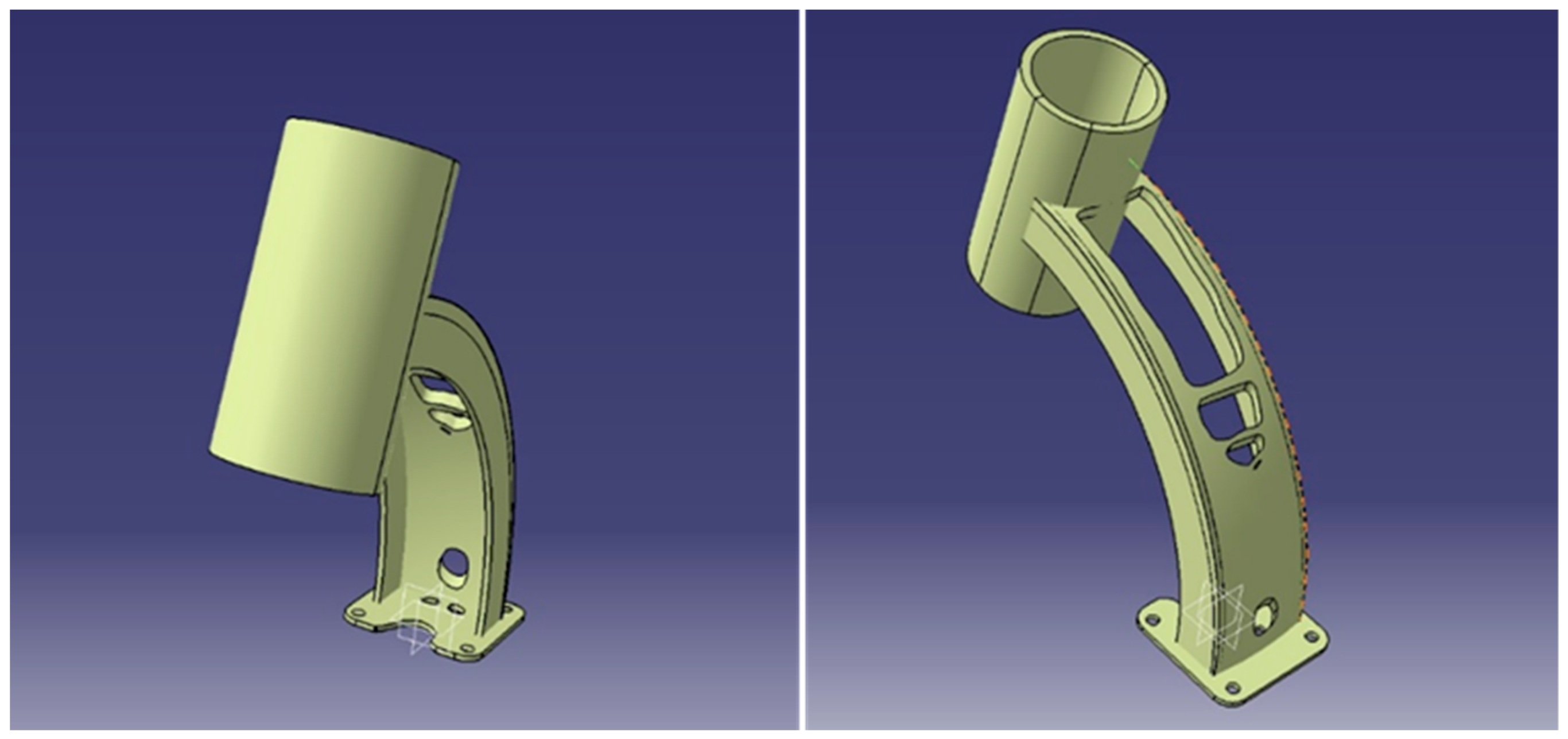
Both alternative methods were methodically applied to the optimized neck geometry prior to the development of the hybrid strategy. The automatic STL-based reconstruction tool (ANSYS SpaceClaim smoothing module) was unable to produce a watertight solid because of non-manifold edges in the SIMP output. The edge-based NURBS reconstruction resulted in patch boundary discontinuities at intricate junction locations, obstructing the formation of a valid B-Rep model. In this case, only the proposed hybrid approach was successful in producing a closed, FEA-compatible CAD model, as outlined in Table 1.

A significant finding from Table 1 is that alternatives are entirely ineffective for this class of geometry, yielding no valid geometry. The proposed hybrid method is the only approach that successfully produced a structurally valid geometry for this class of problem, whereas automated methods failed entirely. 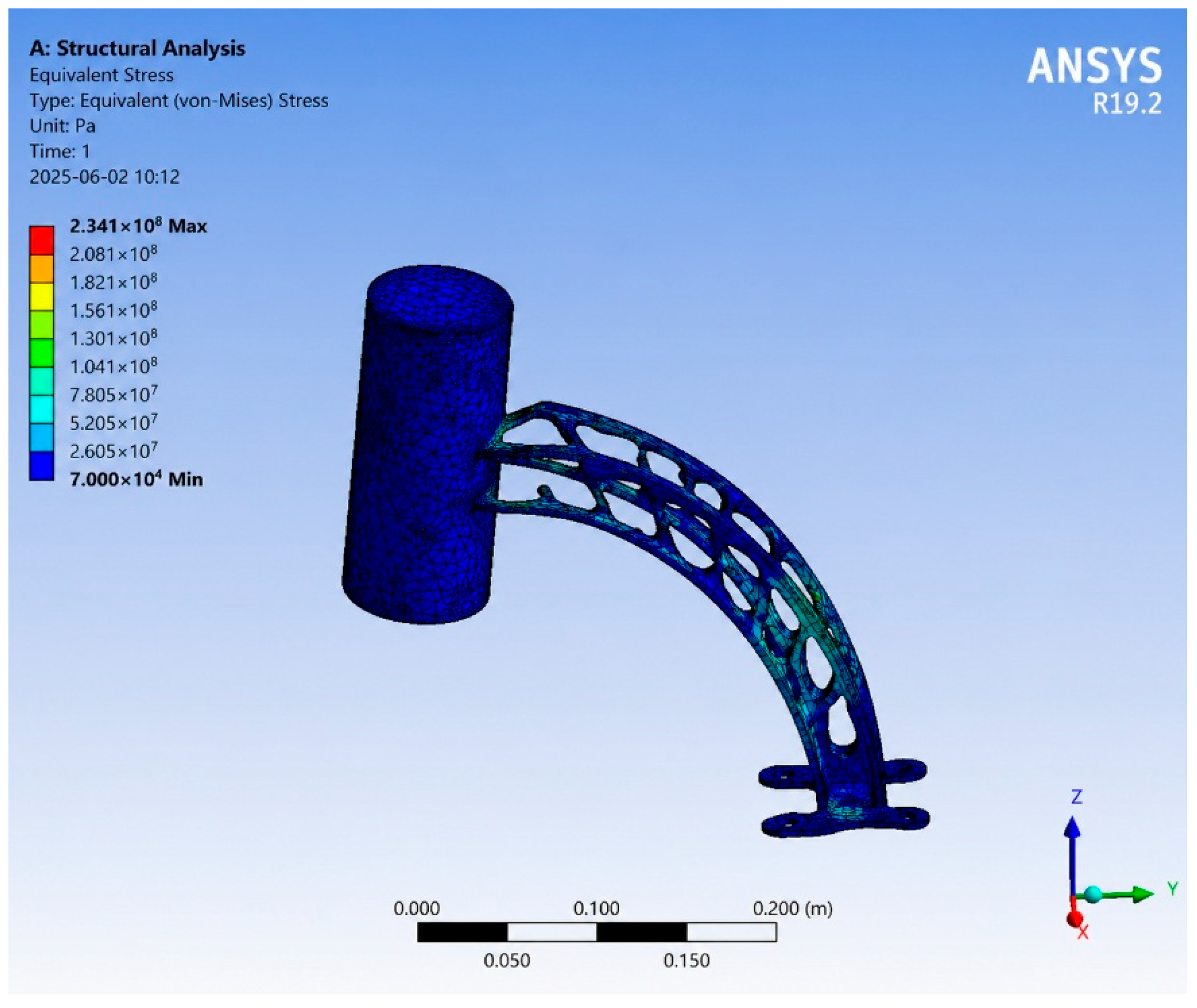Moreover, the transition from the direct SIMP output (${\sigma }_{VM}=201\mathrm{M}\mathrm{P}\mathrm{a}$, $SF=1.37$) to the NURBS-reconstructed geometry (${\sigma }_{VM}=126.45\mathrm{M}\mathrm{P}\mathrm{a}$, $SF=2.18$) demonstrates that reconstruction is not a neutral process—it reduces peak stress by 37.1% and raises the safety factor by 59.1%, neither of which is predictable from the SIMP density field alone.

The basic difference, as opposed to the commercial automated systems, is not in the use of NURBS per se, but in the region-decomposition method used to overcome non-manifold topological failures. The hybrid approach led to a surface error of less than 0.3 mm between the reconstructed NURBS geometry and the original SIMP density field, as calculated by CATIA V5 Digitized Shape Editor deviation analysis. This verified the geometrical accuracy and corrected the topological flaws that impeded the FEA revalidation of the other two methods. The extra processing time (approximately 3.5 h rather than approximately 0.5 h with automated techniques) is justified because automated reconstruction was completely ineffective with this geometry type, making a time comparison impossible. The extra processing time is thus compensated by the fact that the method can provide a structurally validated result where automated methods fail completely.

3. Enhancement of Topology Optimization Workflow by Adopting NURBS on Geometry Reconstruction Phase, Numerical Study and Discussion

3.1. Electric Scooter Neck Overview

This paper presents the computational results and verification of a topology optimization tool used on a scooter neck. The main structural part of the assembly is the neck, as shown in Figure 4. It links the frame of the scooter with the rider. This component is well-suited for lightweight design optimization. Safety and performance are paramount, and performance, thus optimization, should be conducted within strict limits. Urban mobility demands that engineers develop lighter parts to meet the needs of more efficient and portable transport solutions in crowded environments. The lighter component is easier to carry and enhances the overall user experience. Topology optimization is one of the most efficient ways to address this issue, and engineers can develop lightweight structures that are robust and useful and use the minimum amount of material. This strategy affects the way designers contemplate and create items to be produced through additive manufacturing, allowing them to reduce weight without affecting structural integrity or functionality. Reduction in mass is thus a design goal, which directly enhances portability and user experience.

3.2. Electric Scooter Load Case and Material Properties

ANSYS Mechanical R19.2 was used to perform the finite element modeling. The mesh consisted of SOLID187 tetrahedral elements, which are second-order and have better strain resolution properties. These elements are very accurate in the resolution of steep stress gradients. The geometry was that of a standard urban scooter neck, with a length of 550 mm, a width of 150 mm, and a thickness of 8 mm. Four bolted joint locations were incorporated at the neck. This configuration provided a structurally sound mounting system. The midpoint was loaded vertically with a load of −600 N. The force applied was the weight of a typical rider at rest, although the forces due to jumps and maneuvers are more complex, as can be seen in Figure 3.

Symmetry was used to reduce the computational cost. The basic material utilized was 6061-T6 aluminum. It is lightweight, strong, and corrosion-resistant. Its modulus is approximately 68.9 GPa, Poisson’s ratio is 0.33, yield strength is 276 MPa, and density is 2700 kg/m³. These values are in line with the mobility design requirements.

The mesh convergence test was used to reduce the size of the elements gradually until it was 1.25 mm. The solution converged to a mesh size of 2.5 mm with a relative error below 0.5%.

Iterative refinement was used to verify mesh convergence with the same SOLID187 quadratic tetrahedral elements and boundary constraints. The size of the element was reduced to 1.25 mm, and the maximum von Mises stress was changed by 0.90% (126.45 MPa to 127.6 MPa), which is less than the 1% convergence criterion. This confirmed that the 2.5 mm mesh provided mesh-independent results in all the analyses performed in this research. The production mesh was set to 2.5 mm.

The initial setup had the highest stress of 187 MPa, deflection of 1.89 mm, and mass of 1.247 kg. The strain energy was 0.0847 J. These data serve as a baseline for future comparison.

3.3. Topology Optimization of the Neck

Optimization was performed using the SIMP methodology, and the aim was to minimize compliance and meet the density, volume, and equilibrium constraints. The stiffness is given in Equation (15), where $p=3$, a typical value for metallic materials.

The initial optimization step produced a very low volume fraction of 0.20. After 500 iterations, the neck mass decreased to 0.249 kg (Figure 6). However, the peak stress reached 312 MPa, which is more than the yield point. The safety factor was less than one. There were high levels of stress in a number of areas. The outcome was evident: the design was structurally unsound because of the over-removal of materials (Figure 7).

A stress constraint was implemented in the second attempt. When the volume fraction was increased to 0.40, the stress constraint was set to ${\sigma }_{\mathrm{v}}\le 207\mathrm{M}\mathrm{P}\mathrm{a}$. After 428 iterations, the model was completed. The neck had a mass of 0.511 kg. The peak stress was reduced to 201 MPa, which is lower than the yield point. The resulting architecture has more efficient load paths and has better structural reliability (Figure 8).

3.4. Geometry Reconstruction Using NURBS Function

The geometric reconstruction process is organized into four stages:

Stage 1: Contour extraction: The SIMP density field is thresholded at ρ ≥ 0.5 and exported as an STL surface (0.5° angular tolerance; 0.01 mm chord height deviation). Using the CATIA V5 Digitized Shape Editor, principal contour curves are taken from high-curvature ridges. These curves form the guide network for subsequent surface fitting.

Stage 2: B-spline curve fitting: The extracted contours are fitted with a degree-3 B-spline interpolation with a fitting tolerance of ε = 0.05 mm. At all curve intersections, tangent continuity (G1) is required. This stage establishes the parametric framework for constructing the next surface patch.

Stage 3: Building a NURBS surface: The CATIA V5 Freestyle Surface (FFS) module makes NURBS patches of degree (u, v) = (3,3) over the B-spline guiding network. The maximum surface variation for each patch is kept below 0.1 mm in relation to the B-spline network. Automated surface generation is used in prismatic and cylindrical areas, while freeform and junction areas use manually directed multi-section NURBS. There must be at least 2 mm of wall thickness throughout.

Stage 4: Validation and export: The rebuilt solid is checked to verify that it is watertight (there are no edges that are not manifold). The CATIA V5 Digitized Shape Editor deviation analysis measures how far the global surface is from the original SIMP density field. It must be less than 0.3 mm. The approved geometry is exported as STEP AP214 so that it can be re-validated for FEA in ANSYS Mechanical R19.2.

These limitations were addressed by transferring topology-optimized results into CAD-compatible geometry and required delicate manual intervention. Simple geometric operations were used to reconstruct cylindrical regions automatically. More complex areas were extruded and subtracted using Boolean operations. A minimum wall thickness of 2 mm was used to guarantee manufacturability. Continuity was ensured geometrically by rebuilding curved and freeform areas using smooth and continuous NURBS surfaces. This combinatorial method generated a manufacturable CAD model that was subsequently validated, as shown in Figure 9.

3.5. Validation of Optimized Geometry

ANSYS Mechanical R19.2 was used to re-validate the NURBS-reconstructed geometry using the same SOLID187 quadratic tetrahedral elements and a global element size of 2.5 mm. The same boundary conditions as the baseline model were applied: four fixed support conditions at the bolt-hole cylindrical faces and a 600 N vertical force at the handlebar clamp face.

The re-validation results are summarized in

Table 2. Structural performance indices for Al 6061-T6 under a 600 N vertical stationary load, utilizing ANSYS Mechanical R19.2.

Parameter	Baseline	$\mathbf{Iter}.1(\mathit{V}\mathit{f}$ = 0.20)	$\mathbf{Iter}.2(\mathit{V}\mathit{f}$ = 0.40)	NURBS Reconstructed
Mass (kg)	1.247	0.249	0.511	0.531
Mass reduction (%)	—	80.0%	59.0%	57.4%
Max ${\sigma }_{VM}$ (MPa)	187.0	312.0 [FAIL]	201.0	126.45
Safety factor (SF)	1.48	0.88 [<1]	1.37	2.18 ✓
Max deflection (mm)	1.89	—	—	2.31
1st Nat. freq. (Hz)	—	—	—	≈127

. The yield strength of Al 6061-T6 is 276 MPa, which is substantially higher than the maximum von Mises stress of 126.45 MPa. The safety factor is $SF=276/126.45=2.18$. This value meets the engineering criteria of $SF\ge 2.0$ for structural vehicle parts subject to dynamic loading. The maximum deflection of 2.31 mm remains below the design limit of 5 mm. The first natural frequency, approximately 127 Hz, is well above the operating frequency range of the electric scooter (0–30 Hz), thereby precluding resonance.

The NURBS-based reconstruction not only enabled the production of a valid geometry but also considerably reduced the stress concentration, decreasing the maximum von Mises stress from 201 MPa to 126.45 MPa and increasing the safety factor from 1.37 to 2.18.

Note on boundary singularities: stress concentrations at fixed support nodes are well-known numerical artifacts arising from idealized bolted joint representations in FEA. These singularities were found and not included in the reported maximum stress, which was calculated over the whole component.

4. Discussion and Conclusions

A direct volume measurement of the NURBS-reconstructed geometry confirmed a 57.4% mass reduction [(1.247 − 0.531)/1.247 × 100 = 57.4%]. The NURBS-reconstructed volume is 196,505 mm³; when multiplied by the material density of Al 6061-T6 (ρ = 2.7 × 10 ⁻⁶ kg/mm³) this gives m = 196,505 × 2.7 × 10⁻⁶ = 0.531 kg. Achieving precise and cost-effective structural optimization requires accurate geometric representation combined with rigorous structural analysis. The proposed method leverages the geometric fidelity of NURBS—including smooth surface transitions and enhanced interpolation continuity—to address challenges of scalability, precision, and geometric flexibility.

The proposed enhancement of the topology optimization workflow demonstrates that the combination of B-spline and NURBS-based representations can significantly enhance the geometric accuracy and efficiency of the post-processing, as shown in Figure 10.

This method allows a more accurate and easier geometric reconstruction by substituting the traditional polygonal (Lagrange) elements with NURBS-based representations, especially when the reconstruction product will be NURBS-based surfaces.

The use of the method is illustrated through a case study of an aluminum Al 6061-T6 electric scooter neck, which has undergone a confirmed mass reduction of 57.4% without compromising the required structural performance.

These results highlight the utility of this method in achieving sustainability objectives by enhancing the mass reduction and optimization of the structural behavior.

This method adds processing complexity to converting FEM mesh-based data to smooth NURBS geometry.

Structural integrity is confirmed: FEA re-validation yields ${\sigma }_{VM}=126.45\mathrm{M}\mathrm{P}\mathrm{a}<{\sigma }_{yield}=276\mathrm{M}\mathrm{P}\mathrm{a},$ SF = 2.18 (>2.0 requirement), $\delta max=2.31\mathrm{m}\mathrm{m}$ (<5 mm limit), and $f_1$ $\approx 127\mathrm{H}\mathrm{z}$ (above the operating range of 0–30 Hz).

Moreover, the quality of the original FEM model defines the quality of the method; any errors in the FEM solution can thus be transferred to the reconstructed geometry.

Limitations: The study employed a single 600 N static load in a stationary state; additional multi-load case studies and experiments are identified as essential future work. The proven NURBS geometry (STEP AP214 format) is directly compatible with isogeometric analysis frameworks [17,18] and is a natural extension of this work toward IGA-based structural computation.