Article

Integration of Multi-Gas Sensors and Aerial Thermography into UAVs for Environmental Monitoring of a Landfill

by
Juan Francisco Escudero-Villegas
1,
Macaria Hernández-Chávez
1,
Bertha Nelly Cabrera-Sánchez
2,
Gilgamesh Luis-Raya
3,
Josué Daniel Rivera-Fernández
1 and
Diego Adrián Fabila-Bustos
1,*
1
Laboratorio de Optomecatrónica y Energías, UPIIH, Instituto Politécnico Nacional, Distrito de Educación, Salud, Ciencia, Tecnología e Innovación, San Agustín Tlaxiaca 42162, Hidalgo, Mexico
2
Escuela Superior de Ingeniería y Arquitectura Unidad Tecamachalco, Instituto Politécnico Nacional, Naucalpan de Juárez 53950, Estado de Mexico, Mexico
3
Universidad Politécnica de Pachuca, Carretera Pachuca-Cd. Sahagún km 20 Ex-Hacienda de Santa Bárbara, Zempoala 43830, Hidalgo, Mexico
*
Author to whom correspondence should be addressed.
Appl. Sci. 2026, 16(8), 3970; https://doi.org/10.3390/app16083970
Submission received: 23 March 2026 / Revised: 13 April 2026 / Accepted: 15 April 2026 / Published: 19 April 2026

Featured Application

The proposed methodology can be applied to the environmental monitoring of landfills by spatially identifying biogas emissions and surface-level thermal anomalies. Its integration into Unmanned Aerial Vehicle (UAV)-based monitoring campaigns can assist environmental authorities in detecting critical areas and assessing local variability that is not adequately captured by spot monitoring.

Abstract

Landfills are a significant source of atmospheric emissions associated with the decomposition of organic waste; however, conventional monitoring methods typically have limited spatial coverage. This study evaluates the use of an UAV-based system for the spatial characterization of gases associated with biogas emissions at a municipal landfill. A DJI Matrice 350 RTK platform equipped with a Sniffer4D Mini2 multi-gas station and a Zenmuse H20T thermal camera were used. Four flight campaigns were conducted at an altitude of 20 m, with an acquisition frequency of approximately 1 Hz, recording total hydrocarbons (CxHy) as an indirect indicator of methane (CH4), carbon dioxide (CO2), carbon monoxide (CO), nitrogen dioxide (NO2), ozone (O3), sulfur dioxide (SO2), oxygen (O2), temperature, and relative humidity. The results showed a marked transition around 13:10 h, characterized by a simultaneous increase in CH4 equivalent and CO2, along with a decrease in NO2, O3, and SO2. Furthermore, CH4 equivalent and CO2 showed the highest positive correlation among the variables (r = 0.96). Spatial maps generated using ordinary kriging revealed more heterogeneous patterns, while the qualitative thermal orthophoto confirmed the site’s surface variability. Overall, the results demonstrate that the integration of multi-gas sensors and aerial thermography on UAVs is viable for the spatial monitoring of landfills.

1. Introduction

The emission of pollutants and greenhouse gases into the atmosphere represents one of the most significant environmental challenges today due to its impact on climate change, air quality and human health. Among anthropogenic sources, landfills are a significant source of gas emissions due to the anaerobic degradation of organic waste. This process produces biogas composed mainly of methane (CH4), typically ranging from 40% to 70% and carbon dioxide (CO2), typically 30% to 60%, along with other trace compounds such as hydrocarbons, carbon monoxide (CO), nitrogen oxides (NOx), and sulfur dioxide (SO2) [1,2]. Methane is particularly relevant from a climate perspective because its global warming potential is significantly higher than that of CO2 over short time scales, making landfills an important source of greenhouse gas emissions [3].
The quantification and spatial characterization of these emissions are essential for improving waste management practices and developing effective mitigation strategies. However, traditional monitoring methods based on fixed stations or point measurements present significant limitations in spatial coverage and temporal resolution, especially in large or difficult-to-access facilities [4]. Although such systems provide reliable time series, they often fail to capture spatial variability or accurately identify emission hotspots and leakage zones. Currently, the development of unmanned aerial vehicles (UAVs) has opened up new opportunities for high-resolution environmental monitoring. These platforms enable flexible atmospheric measurements in the lower boundary layer and allow the integration of compact sensors for the detection of multiple gases [5,6].
Numerous studies have demonstrated that UAVs can be used to obtain vertical gas profiles, track emission plumes, and characterize the spatial distribution of atmospheric pollutants in complex or difficult-to-access environments [7,8]. Advances in the miniaturization of electrochemical, infrared, and spectroscopic sensors have enabled their integration into multirotor platforms, allowing the simultaneous measurement of multiple gases, including CO2, CH4, CO, NO2, O3, SO2, during atmospheric monitoring campaigns [9].
Within this context, one of the most dynamic applications of UAVs is the monitoring of methane emissions in waste management facilities and the energy sector. Previous studies have shown that aerial systems equipped with gas sensors can detect emission sources and estimate methane fluxes using approaches such as mass balance methods and low-altitude concentration mapping [10,11]. In addition, the use of thermal sensors mounted on UAVs has proven to be a useful tool for identifying thermal anomalies associated with biogas migration, enabling the identification of potential leakage zones in landfills [12]. These combined approaches enhance the detection of emission hotspots and complement conventional monitoring techniques. However, despite recent advances, most studies have focused primarily on methane or carbon dioxide, whereas investigations that simultaneously consider multiple atmospheric pollutants associated with biogas remain limited. Therefore, the integration of multi-gas sensors into UAV platforms offers a valuable means to achieve a more comprehensive characterization of landfill emissions and to improve the understanding of interactions among biogas generation processes, localized combustion and atmospheric conditions.
Therefore, this study aims to evaluate a UAV-based atmospheric monitoring system equipped with a portable multi-gas station for the spatial characterization of gases associated with biogas emissions [11]. To achieve this, measurement campaigns were conducted using a UAV-mounted environmental monitoring system capable of recording concentrations of CxHy, CO2, CO, NO2, O3, SO2, O2, as well as meteorological parameters such as temperature and relative humidity. In addition, thermal images were acquired using an infrared camera integrated into the UAV to identify possible thermal anomalies associated with biogas emission processes. Based on these data, spatial distribution maps of gases were generated to detect possible accumulation zones and analyze the feasibility of using a combination of UAVs, multi-gas sensors and aerial thermography as a tool for landfill environmental monitoring.

2. Materials and Methods

The acquisition of atmospheric data using unmanned aerial vehicles has proven to be a useful alternative for studying the lower atmosphere and for environmental monitoring in locations where ground access is limited or where the spatial variability of emissions makes it difficult to characterize them using conventional point measurements [4,5]. The integration of miniaturized sensors into these platforms has enabled simultaneous monitoring of different atmospheric variables and trace gases, facilitating the analysis of emissions and their spatial distribution in various environments [6,13].
In the particular case of landfills, this approach is especially relevant due to the heterogeneous nature of gaseous emissions and the need to integrate spatial, thermal, and meteorological information within a single measurement campaign [1,2,12].
This section describes the materials, instrumentation, and procedures employed for data acquisition and processing. First, the study area and its main characteristics are presented, followed by a description of the UAV platform, the multi-gas monitoring system, and the thermal sensor used during the campaigns. Finally, the flight planning criteria are outlined, along with the data processing, quality control, and geospatial integration given that this type of study requires a robust association between the position of the UAV, the atmospheric variables measured, and the spatial analysis tools [13,14].

2.1. Study Site

The study was conducted at a municipal solid waste (MSW) disposal site located in central Mexico, east of the State of México. The site is situated at an average altitude of approximately 2544 m above sea level, within the central Mexican highlands. The surrounding area is predominantly mountainous, with variations in altitude that influence local climatic conditions, characterized by a temperate climate and gentle slopes at the disposal site.
The landfill operates as a regional infrastructure for the final disposal of municipal solid waste, resulting from an inter-municipal management scheme established with the aim of improving waste management in the region [15]. This operating model was formalized through institutional agreements and subsequently through the creation of a decentralized public body responsible for managing the site [16]. At the institutional level, this type of facility is part of the regional waste management systems recognized in national assessments of urban solid waste infrastructure in Mexico [17].
The site mainly receives municipal solid waste from domestic and commercial sources, which is deposited and compacted in designated disposal cells. Due to the anaerobic degradation processes of the organic fraction of the waste, biogas is generated, composed mainly of CH4 and CO2, in addition to other gaseous compounds present in lower concentrations. The evaluated site does not have an active biogas capture or utilization system, which may favor the diffuse release of gases into the atmosphere.
The topographical characteristics of the study area, together with the absence of biogas collection systems and the heterogeneous nature of the landfill surface, can generate complex spatial patterns of gas emissions, including areas of localized biogas accumulation or release. Due to this spatial variability, the site represents a suitable environment for the application of atmospheric monitoring techniques based on unmanned aerial vehicles (UAVs), which enable the characterization of the spatial distribution of pollutant gases.

2.2. UAV Platform

A DJI Matrice 350 RTK unmanned aerial vehicle (DJI, Shenzhen, China) was used for data acquisition. It is an industrial-grade multirotor platform designed for professional environmental monitoring, inspection, and geospatial surveying applications. It has proven particularly suitable for environmental studies due to its flight stability, payload capacity, and capability to integrate multiple sensors for measuring atmospheric and environmental variables [4].
The Matrice 350 RTK incorporates a navigation system based on Real-Time Kinematic (RTK) technology that allows centimeter-level accuracy in the georeferencing of data acquired during flight. This system can provide horizontal accuracies close to 1 cm + 1 ppm and vertical accuracies of 1.5 cm + 1 ppm, facilitating the correct spatial integration of atmospheric measurements obtained during monitoring campaigns. This type of positioning capability is essential when conducting environmental characterization studies using UAV platforms [5,6]. The platform has a weight of approximately 6.47 kg, dimensions of 810 mm × 670 mm × 430 mm and a flight endurance of up to 55 min under no-payload conditions. It can reach a maximum speed of 23 m/s and is equipped with a global positioning system compatible with GPS, Galileo, BeiDou, and GLONASS, enhancing positioning stability during flight operations. These characteristics make this type of platform suitable for environmental monitoring and high-precision geospatial surveying applications [5].
During the measurement campaigns, the UAV was equipped with two sensing systems. A Sniffer4D Mini2 (AIRINS, East Region, Singapore) multi-gas environmental monitoring analyzer (approximately 400 g) was mounted on the upper section of the UAV to measure various atmospheric pollutants. Conversely, a DJI Zenmuse H20T thermal camera (DJI Technology Co., Shenzhen, China) was installed on the lower section to acquire thermal information from the surface of the study site. Flight operations were carried out at an approximate height of 20 m above ground level to obtain representative measurements of gas concentrations and atmospheric conditions present in the study area. A total of four flights were performed, each lasting approximately 15 min. Data generated by the monitoring system were recorded at a temporal frequency close to 1 Hz, determined from the time interval present in the records exported in CSV format, which allowed a continuous time series of the variables monitored during each measurement campaign to be obtained. The main characteristics of the UAV platform used in this study are presented in Table 1.

2.3. Gas Monitoring System

A Sniffer4D Mini2 multi-gas monitoring system, specifically designed for integration into UAV platforms and for real-time environmental data acquisition, was used to measure atmospheric gases during flight campaigns. The use of gas sensors mounted on unmanned aerial vehicles has been widely reported as an effective tool for monitoring fugitive emissions in landfills and other industrial environments, due to their ability to measure with high spatial resolution and detect local variations in gas concentrations [4,6,12].
The Sniffer4D Mini2 system allows the simultaneous detection of various gases by integrating different sensing technologies within a single compact module. In this study, the system was configured to measure CxHy, CO2, CO, NO2, O3, SO2 and O2, as well as to record environmental variables such as temperature and relative humidity, which are relevant for interpreting atmospheric dynamics and pollutant dispersion.
Total hydrocarbons were detected using a sensor based on non-dispersive infrared (NDIR) technology, which quantifies the combustible gases present in the biogas produced by the decomposition of organic waste. Due to its stability, selectivity, and ability to detect gases such as methane over relatively wide concentration ranges [7], this type of sensor is frequently used in environmental applications. For the system used, the hydrocarbon measurement range was 0–5% VOL (equivalent to 0–100% of the lower explosive limit, LEL) for CH4 or 0–2% VOL for propane (C3H8), with a theoretical resolution of 0.01%. Measurements of CO, NO2, SO2 and O2 were performed using electrochemical sensors, a technology frequently employed in environmental monitoring due to its high sensitivity for detecting trace gases at relatively low concentrations. In particular, the oxygen measurement module allows for the quantification of concentrations between 0 and 50%, with a detection limit close to 1% and a theoretical resolution below 0.1%. This enables the assessment of changes in atmospheric composition linked to biological and oxidation processes occurring in landfills.
The system also includes a combined O3 + NO2 measurement module that uses electrochemical technology and responds simultaneously to both oxidizing compounds. This type of sensor measures the total concentration of atmospheric oxidants, making it possible to calculate the individual O3 concentration by subtracting the amount of NO2 measured by its own sensor from the total signal (NO2 + O3). We can calculate the ozone concentration using the following formula:
O 3 = O 3 + NO 2   NO 2 ,
This procedure is standard in environmental monitoring systems that use electrochemical sensors, and it enables the calculation of ozone concentrations in air quality studies and atmospheric monitoring. However, CO2 was measured using NDIR technology, which has a measurement range of up to 50,000 ppm. This allows for the recording of concentration fluctuations related to the organic degradation processes occurring in landfills.
By integrating with the UAV’s GNSS system, the system continuously recorded gas concentrations and geographic locations during flights, generating time-series data with geographic references. The data were then exported in CSV format for processing and analysis. This ensured that each concentration measurement was associated with its corresponding spatial location, enabling the creation of gas distribution maps for the study area. The main technical specifications of the gas monitoring system used are presented in Table 2.
Total hydrocarbons were detected using a sensor based on non-dispersive infrared (NDIR) technology, a technique that enables the quantification of combustible gases in the biogas produced by the decomposition of organic waste. For hydrocarbons, the measurement range in the system used was 0 to 5% VOL (0 to 100% of the lower explosive limit or LEL) for CH4 or 0–2% VOL for C3H8. The detection limit was close to 0.01% (100 ppm), and the approximate response time was t90 < 30 s.
The CxHy/CH4/LEL sensor is set by default to measure CH4, one of the main components of the biogas generated in landfills due to the anaerobic degradation of organic waste. Given this configuration, the CxHy measurements recorded by the system primarily estimate of atmospheric methane concentration, particularly in contexts where this gas is the major component among the hydrocarbons present. In this study, CxHy concentrations served as an indirect indicator of methane presence, facilitating the identification of potential areas where biogas could be released or accumulate within the study area.

2.4. Thermal Capture System

To observe temperature fluctuations on the surface of the study area, a thermal camera that operates with infrared radiation is essential. In this project, the thermal camera identifies thermal patterns that may be associated with sources of gas emissions or changes in the terrain that are not visible to the naked eye. As noted in the work by Fosco et al. [1], this technology commonly detects sources of pollution and investigates the environment, specifically in the case of methane emissions from landfills using unmanned aerial vehicles (UAVs) equipped with high-resolution thermal cameras.
The camera selected for this study is the Zenmuse H20T from the UAV system, which combines high-definition thermal imaging with a wide range and the ability to capture accurate temperature data. This camera can generate detailed thermal maps that help detect “hotspots” or areas with a higher concentration of gases, which is essential for quantifying emissions.

2.5. Planning of UAV Flight Campaigns

Proper planning of flight missions is essential to ensure the quality and reproducibility of data collected by drones, particularly when thermal and gas sensors are incorporated into environmental monitoring studies. According to several authors, photogrammetric accuracy and thermal resolution are directly affected by the precise establishment of routes, flight altitudes, capture modes, and spatial coverage [18]. The measurement campaign was organized following a systematic protocol using DJI Pilot 2 software v2.5.1.15, which is built into the UAV’s remote control. This enabled the safe and effective planning, execution, and monitoring of flights.

2.5.1. Creating the Flight Plan

The flight path tool within the DJI Pilot 2 interface was used to plan the flight campaigns. Next, a georeferenced polygon was drawn to precisely define the area of interest where measurements would be taken. This polygon ensured the UAV operation remained within safe and permitted limits and provided uniform coverage during data acquisition.
Once the area had been determined, a grid-based or systematic flight path was automatically generated, allowing the entire defined area to be covered evenly. To ensure a more stable flight and enable representative dispersion of the gases detected by the sensors, various operational and environmental factors were considered during mission planning, particularly the direction and speed of the prevailing wind in the region. In addition, a flight altitude of 20 m above ground level was set to ensure appropriate proximity to the surface without compromising the UAV’s operational safety or the quality of the measurements.
The flight path consisted of a series of parallel lines that completely covered the designated area; this method is widely used in environmental monitoring studies involving UAVs, as it ensures that data are evenly distributed throughout the entire area of interest [19]. This flight pattern allows the UAV to perform a systematic sweep, continuously recording gas concentrations. Figure 1 shows an example of the planned flight path, illustrating the operational area and the flight routes taken by the drone to collect data.

2.5.2. Selection of Sensor Configuration and Capture Type

The Matrice 350 RTK aerial platform and the corresponding image capture system were configured after defining the flight polygon. In this case, data acquisition was performed using the optical sensor mounted on the aircraft. Priority was given to capturing high-resolution images for subsequent photogrammetric processing to create georeferenced orthomosaics. The inclusion of the RTK positioning system increased the spatial accuracy of the generated products, thereby reducing uncertainty regarding the location where each image was captured.
An automated flight path with a strictly nadir orientation (90° relative to the ground) was selected to meet the geometric requirements necessary for producing orthomosaics. This configuration is essential for improving spatial modeling accuracy during photogrammetric processing [20], ensuring adequate longitudinal and lateral overlap between images, and minimizing geometric distortions.

2.5.3. Flight Parameters: Altitude, Speed and Capture Angle

The flight parameters were established in accordance with criteria based on technical recommendations for low-altitude environmental studies [21]. These parameters were chosen to maximize thermal resolution and ensure adequate coverage throughout the study area, without compromising the UAV’s operational stability.
All the parameters configured for this study—such as flight speed, altitude, and camera angle—are essential for properly acquiring and processing thermal and atmospheric data. They are shown in Table 3.

2.5.4. Mission Execution and Data Recording

The automated mission was carried out after the flight parameters were configured. The UAV followed the predefined route, recording data at regular intervals set by the control software. At the same time, the Sniffer4D Mini2 monitoring station recorded gas concentrations and GNSS coordinates. This synchronized operation enabled effective integration of both datasets during geospatial processing and subsequent analysis, ensuring an accurate correlation between the captured imagery and the gas concentration data.

2.6. Data Processing and Analysis

A data processing and analysis phase was conducted following the completion of the four monitoring campaigns, with the aim of ensuring temporal consistency, comparability among variables, and the reliability of statistical and spatial results. Data were collected at a frequency of 1 Hz during the missions, which enabled a continuous time series of the monitored variables. Subsequently, a database cleaning process was carried out to remove invalid values, inconsistencies, and records that were not suitable for analysis. As a result, a final dataset of 3600 clean, georeferenced data points was produced. This comprehensive workflow encompassed database cleaning, standardization of concentration units, statistical concentration assessment, exploratory time-series analysis, and spatial preprocessing for the creation of interpolated maps. In environmental studies, this type of procedure is highly recommended, as the quality of the analysis depends largely on the quality and consistency of the input data [22,23].

2.6.1. Data Preprocessing

Initially, the original file was reviewed to correct formatting inconsistencies and properly organize the dataset. Specifically, the “Time Stamp” column was corrected by removing residual characters and encoding inconsistencies that prevented it from being properly converted to date and time format. Next, only the variables necessary for the analysis were selected: temperature, relative humidity, SO2, NO2, O3 + NO2, CO2, CO, O2, and CxHy/flammable gases. Additionally, the pressure variable was also included because it was used to perform the necessary conversions for certain parameters. Columns not used in subsequent processing were removed to simplify the organization of the dataset and prevent redundancies. Moreover, the main fields were checked for empty or inconsistent records, in accordance with the general quality control criteria typically applied to environmental and monitoring series [22].

2.6.2. Standardization of Units and Calculation of Variables

Since the gas variables from the monitoring system were originally expressed in different units, it was essential to standardize them to express all concentrations in a common unit. To this end, μg/m3 was used as the standard unit. This decision made it possible to compare and interpret the various chemical species on the same physical scale, which is particularly beneficial in studies where multiple pollutants are measured simultaneously.
For CO, which was initially reported in mg/m3, a direct conversion to μg/m3 was performed. For O2 and CxHy, whose readings were recorded as percentages, the conversion was performed using the ideal gas law, taking into account the temperature and pressure measured at each observation and the corresponding molecular weight. For spatial representation and standardization, the CxHy signal was treated as if it were equivalent to methane. This adjustment provides a consistent physical basis for the analysis, particularly when combining variables initially expressed as volume fractions with others reported as mass concentrations.
In addition, the ozone concentration was calculated based on the difference between the combined O3 + NO2 signal and the standalone NO2 signal. Therefore, only the combined variable served as an intermediate input; the subsequent analysis used individual O3 and NO2 concentrations, as this operation allows for clearer interpretation of each compound’s behavior.

2.6.3. Time Series and Exploratory Data Analysis

After structuring the database, an exploratory analysis was conducted to identify overall patterns, variations over time, and possible relationships between the variables. Individual time series were generated for each gas, as well as a combined series that facilitated the simultaneous observation of concentration trends throughout the monitoring period. It should be noted that the time series presented in this study do not correspond to fixed-point temporal monitoring. Instead, they represent sequential measurements acquired along the UAV trajectory, where each timestamp is associated with a different spatial location. Therefore, the observed temporal variations should be interpreted as a combination of spatial variability and temporal evolution during the scan.
Additionally, since some variables exhibited vastly different magnitudes, a scaled representation using z-scores was also developed; this was used solely to facilitate the visual comparison of trends, without neglecting the environmental interpretation based on the original concentrations.
Histograms, box plots, and correlation matrices were also generated. Specifically, the correlation map was created using only standardized gas concentrations, while temperature and relative humidity were examined as auxiliary environmental variables. They were therefore considered in the interpretive analysis using scatter plots and separate maps [23] although these variables are not pollutants in themselves, they can affect the accumulation and dispersion of gases.

2.6.4. Identifying Outliers

The interquartile range criterion (IQR) was used, a method often used to detect observations that deviate considerably from the general trend in dataset [23]. In particular, outliers were defined as those that exceeded Q3 + 1.5 IQR or fell below Q1 − 1.5 IQR. However, these records were not automatically erased, as in environmental monitoring, peak concentrations are not always caused by instrument failures but may be the result of actual short-term emission events. These extreme values may be related to localized emission areas, temporary feather capture or sudden changes in gas accumulation conditions within the framework of landfill gas monitoring. For this reason, although the outliers were noted, they were preserved in the original dataset for analysis.

2.6.5. Spatial Processing of Data

To ensure that each record had a valid and consistent location, the original geographic coordinates were validated prior to any interpolation in the spatial phase. The data were then converted to a projected reference system in meters, which enabled proper handling of spatial distances when creating interpolated surfaces. This step is particularly crucial in geospatial methods such as kriging and IDW, as both rely on the spatial relationship between sampling points [24,25].
The final cartographic products were created using relative local coordinates to avoid publicly disclosing the study site. This made it possible to maintain the validity of the analysis and the spatial geometry of the data without compromising the confidentiality of the actual location of the monitored area.

2.6.6. Spatial Interpolation and Map Generation

To spatially represent the distribution of concentrations, ordinary kriging was applied to the gas variables and as auxiliary environmental variables, to temperature and relative humidity. This method estimates the value at an unsampled location as a weighted linear combination of neighboring observations, according to the following expression:
Z ^ x 0 = i = 1 n λ i Z x i
where:
Z ^ x 0 = is the estimated value at the location x 0 .
Z x i = corresponds to the values observed at nearby points.
λ i = represents the weights assigned to each observation.
In ordinary kriging, these weights are determined based on the spatial dependence structure described by the semivariogram and satisfy the condition of unbiasedness λ i = 1 . To provide a preliminary visual reference during processing, maps were generated using the Inverse Distance Weighting (IDW) interpolation method. This method offers an initial visual approximation of the spatial pattern of the data and serves as a useful starting point [25]. However, these maps were used only for exploratory purposes and were not included in the final presentation of the results.
Therefore, the maps presented in this study are based solely on ordinary kriging. This method was chosen because of its ability to account for the spatial autocorrelation of the data and to generate more consistent surfaces for environmental analysis [24,26].
To preserve the privacy of the study site and ensure visual clarity, the maps were created using relative coordinates, with a uniform design and no direct spatial references.

2.7. Thermal Image Processing and Qualitative Orthophoto Generation

The thermal images obtained during the flight were processed to produce a continuous spatial representation of the surface thermal response of the monitored area. It has been reported that the use of thermal images obtained via UAVs is a useful tool for detecting anomalies on the surface of landfills, as it allows for the identification of areas with different thermal behavior that could be linked to decomposition processes, gas migration, or changes in surface and moisture conditions [27,28]. However, several authors advise caution when interpreting this type of data, as the recorded thermal response also depends on factors such as incident radiation, material emissivity, sensor temperature, and environmental conditions at the time of acquisition [28,29].
In the initial stage, the images were processed in WebODM v2.9.4, following a general photogrammetric workflow that included importing the images, aligning the available spatial data, reconstructing the scene, and creating a georeferenced thermal orthomosaic. This methodology aligns with the workflows reported for UAV-derived photogrammetric products, in which OpenDroneMap-based (Open Source Project, USA) tools enable the creation of elevation models, orthomosaics, and other spatial products from aerial images, using an open and reproducible processing environment [28,30]. The primary product of interest in this research was the thermal orthomosaic, which was used as the basis for the spatial interpretation of the site’s surface thermal response.
Next, for cartographic preparation and final visualization, the orthomosaic exported from WebODM was processed in Python v3.14. In general terms, this stage involved reading the raster, cropping it to the area to be analyzed, configuring a color scale to highlight spatial contrasts, and producing the final figure using relative coordinates. The goal of this processing was not to recover absolute temperatures, but rather to improve the visual interpretation of the surface’s thermal behavior and simplify its comparison with the interpolated gas maps obtained in the study. According to the literature, in the absence of specific corrections for emissivity and environmental conditions or a robust radiometric calibration, the thermal product is more suitable for relative or qualitative analysis than for a strictly quantitative temperature estimate [29,31].
Consequently, the thermal orthophoto produced in this study was interpreted as a qualitative orthomosaic of relative thermal response, which serves to distinguish areas with higher or lower apparent thermal intensity within the study area. This methodological approach allowed the thermal information to be integrated as a supplementary layer to the gas analysis, without having to assign absolute surface temperature values to the image, which could lead to overinterpretation of the landfill’s thermal behavior.

3. Results

To provide a comprehensive interpretation of the analyzed area, the results are presented according to various levels of analysis. In the first stage, we analyzed variations in concentration, sudden transitions, and patterns that might be common across species to understand the temporal behavior of the recorded gases. Next, we used normalized series, correlation matrices, box plots, and histograms to study the dispersion and statistical relationships among the variables. Finally, to identify surface contrasts within the site, we used ordinary kriging interpolation and supplemented it with a qualitative thermal orthophoto. Through this sequence, we were able to link the temporal changes in air composition to their spatial expression within the landfill and identify areas that might be affected by processes related to biogas emissions.

3.1. Temporal Behavior of Gas Concentration

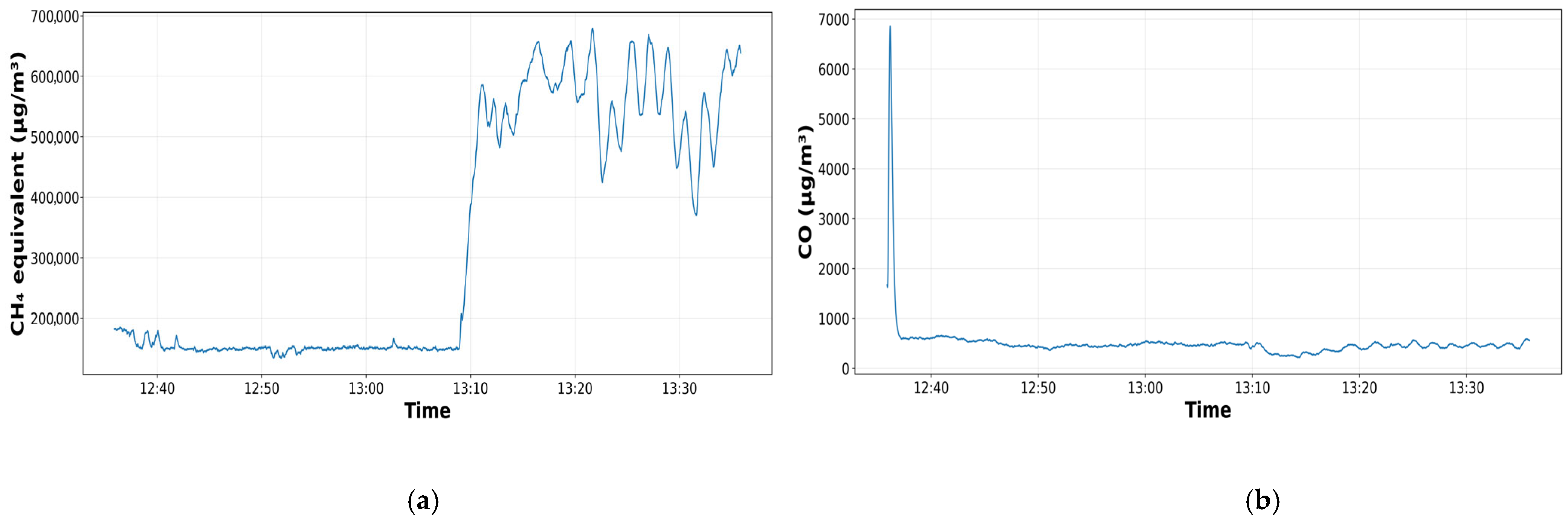
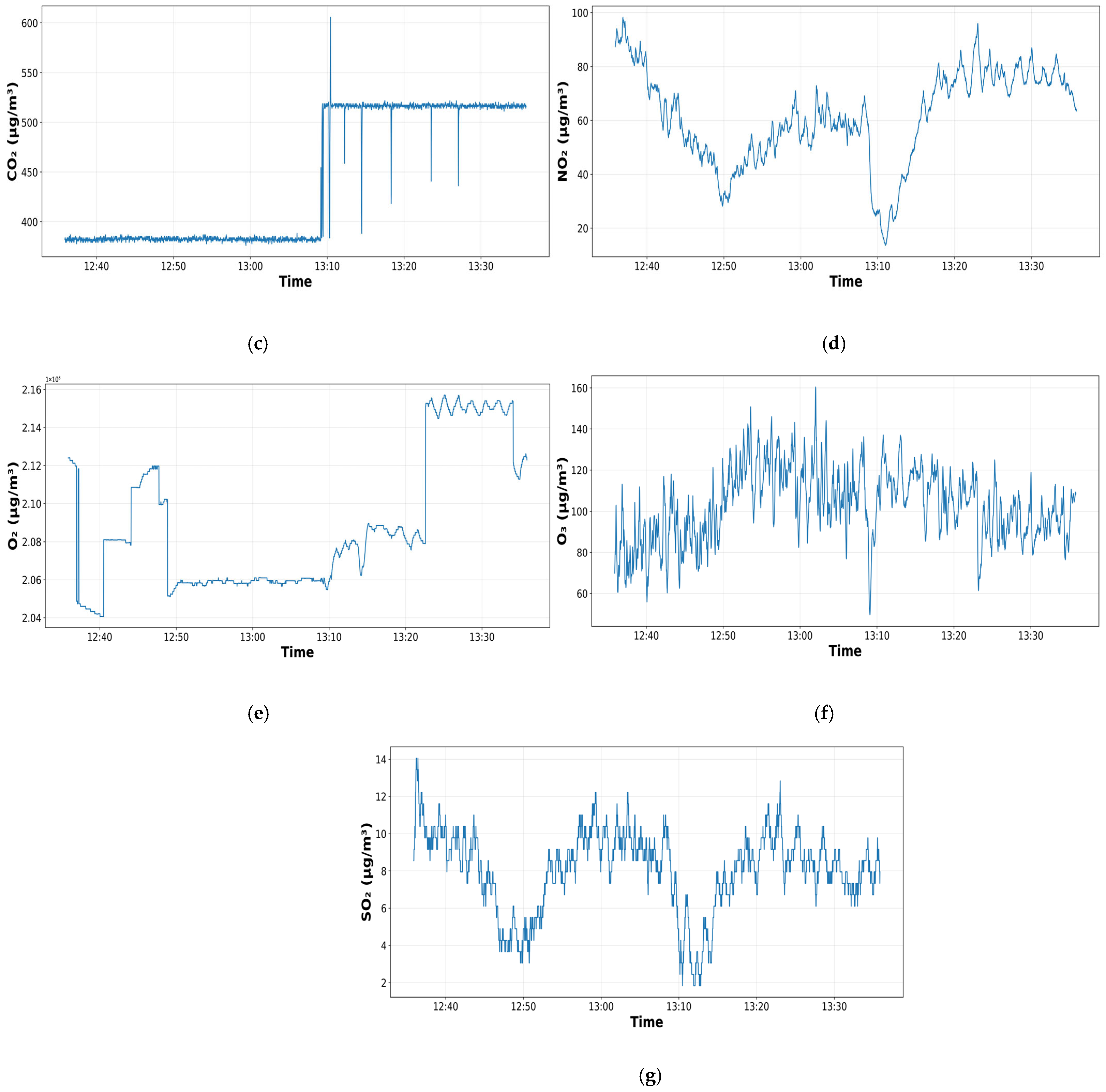
Through a chronological analysis of the measurements, we examined the variability of gas concentrations recorded in the monitoring mission. This included sudden changes, periods of relative stability and possible response patterns among the studied species. It is important to note that these data are not fixed-point time series, as they were collected sequentially as the UAV moved along the predefined air path. Therefore, the trends that are visualized in Figure 2 should be seen as successive observations where time is also related to spatial displacement within the monitored area.
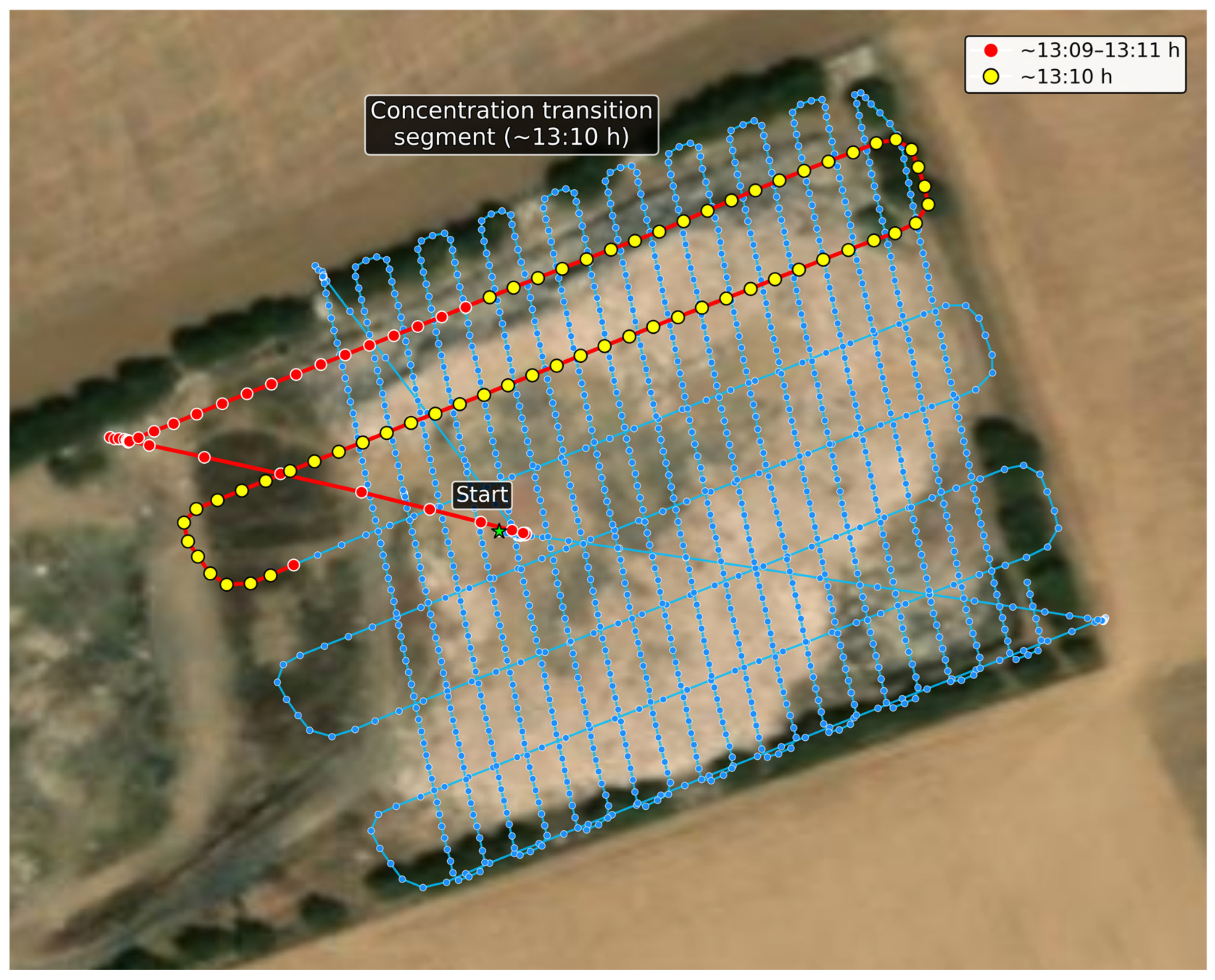
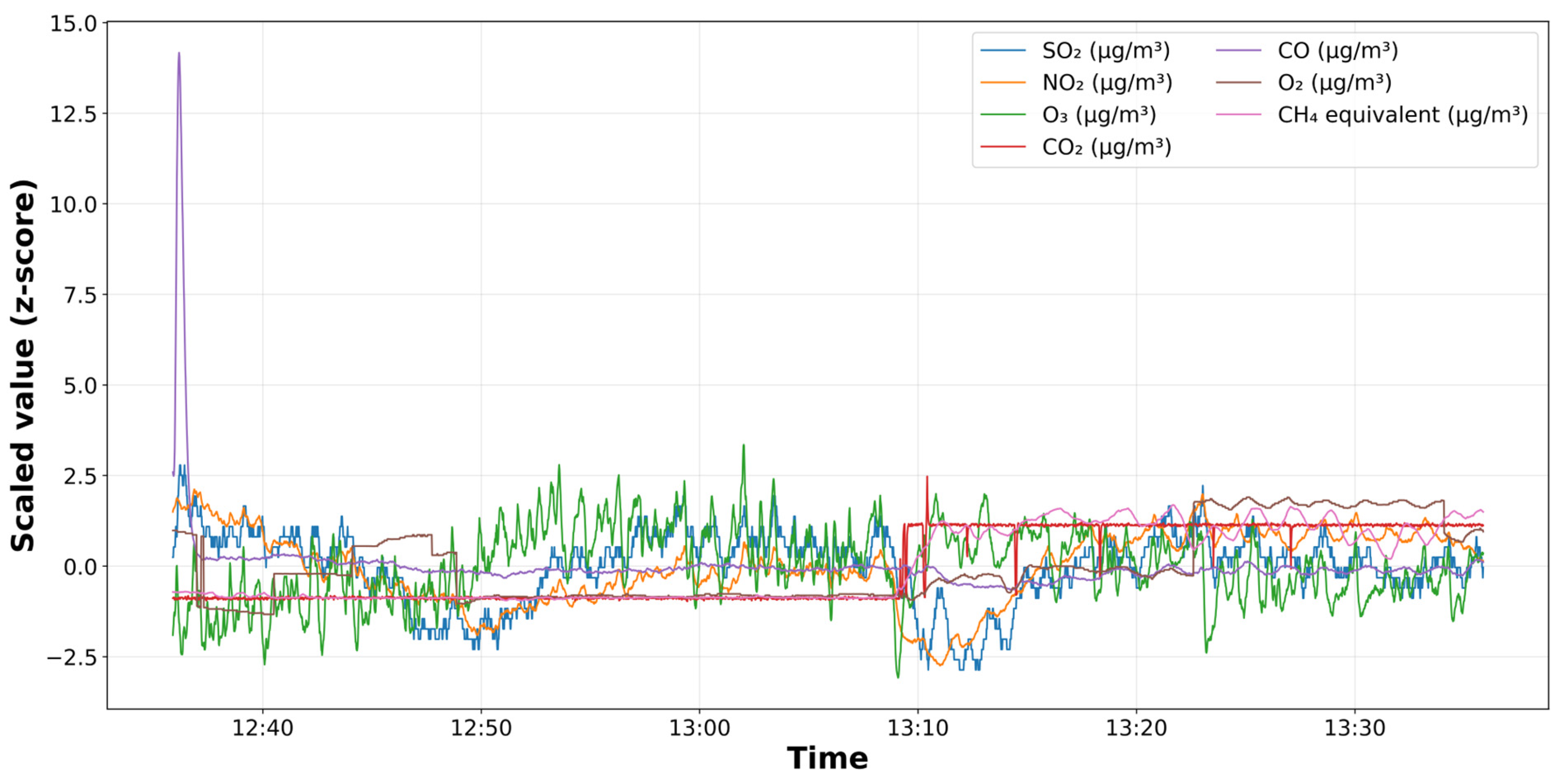
The transition seen at 13:10, shown in Figure 2, is a particular segment of the UAV trajectory, rather than measurements at a given location. During this time, the UAV made flights in adjacent areas within the same general region of the monitored area. Consequently, the increase in CO and CH4 observed around 13:10 was not an isolated event; instead, it extended to subsequent sequential records acquired in adjacent areas.
An initial phase of CH4 (Figure 3a) is observed that remains relatively stable, with concentrations fluctuating between approximately 145,000 and 180,000 µg/m3. Then, at 13:10 h, a sudden increase is observed, raising the signal to a new level, where it experiences fluctuations ranging from approximately 420,000 to 680,000 µg/m3. This change is not the result of an isolated variation, but rather a sustained transition that persists throughout much of the remaining data. The flight segment highlighted in Figure 2 indicates that this transition occurred when the UAV was passing through a specific area of the monitored area, which supports its interpretation as a localized change with spatial association rather than merely a temporal variation at a given site.
A different pattern can be observed for CO (Figure 3b). At the start of the recording, there is a very sharp peak with values close to 6900 µg/m3, which then drops rapidly to a much more stable range, between 400 and 700 µg/m3. From that point on, the signal shows moderate fluctuations, rather than a sustained increase like the one observed for CH4. This alteration conforms to the same section of the UAV’s route, as illustrated in Figure 2, which consolidates the spatial interpretation of the observations.
On the other hand, the CO2 signal (Figure 3c) reveals one of the most evident patterns throughout the entire campaign. During the first part of the monitoring period, concentrations remained nearly stable at around 382 to 384 µg/m3. However, at 13:10 h, there is a clear jump to a new level of around 515–518 µg/m3. After that transition, the series continues within that range, despite some isolated drops and sporadic peaks. In the case of NO2 (Figure 3d), the trend is more variable and gradual. The series begins with fairly high concentrations, ranging from 85 to 95 µg/m3, and then gradually decreases to around 30 µg/m3. There is then a partial recovery; however, at 13:10 h, there is another significant drop, with levels falling to less than 20 µg/m3. After this, there is a steady increase until levels reach between 70 and 85 µg/m3. In contrast to CO2 and CH4 equivalent, the behavior of NO2 is less predictable and more gradual than sudden.
O2 behavior (Figure 3e) should be carefully assessed because its absolute concentration is much higher than that of the other species. Nonetheless, the time series allows for the identification of several relatively unique behavioral patterns throughout the monitoring period. After a noticeable shift at 13:20 h, the signal shows initial decreases, staggered recovery periods, and a higher and relatively stable level.
The O3 time series (Figure 3f) shows a highly irregular signal that frequently fluctuates between 60 and 160 µg/m3. Unlike the corresponding CO2 or CH4 data, no such marked change is observed; instead, there are points in the middle of the record where relatively higher values and rapid, intermittent drops are recorded, especially around 13:10 h. In contrast, the range of change for SO2 (Figure 3g) is smaller, approximately between 2 and 14 µg/m3, with mild oscillations throughout the entire period under investigation. Despite not being the main signal among the observed gases, it exhibits a clear temporal pattern, with an initial progressive reduction, a subsequent recovery, and a notable dip in the interval around 13:10 h.

Integrated Analysis of Temporal Variability

To assess their relative fluctuations on a comparable scale, an integrated comparison of gas concentrations was conducted using z-score normalization, in addition to individual analysis of the time series. This process was necessary because it is difficult to directly compare the monitored parameters in their original units due to differences in order of magnitude between them. Some variables, such as O2 and CH4 equivalent, fluctuate within much narrower ranges, while others, such as SO2, NO2, and O3, reach significantly higher levels. In this regard, standardization allowed for a comparison of temporal changes and signal shapes without the absolute magnitude influencing the interpretation.
Each data point is transformed in relation to the mean and standard deviation of its series as part of z-score normalization. Each variable is therefore expressed in terms of standard deviations and centered around zero. Consequently, concentrations above the corresponding series’ mean are indicated by positive values, and concentrations below that mean are indicated by negative values. As a result, this representation aims to compare the relative intensity of each gas’s temporal fluctuations in relation to its average behavior rather than absolute concentration levels.
Figure 4 shows the combined time series of the normalized variables. Overall, this graph reveals that the monitoring data show a clear transition point at approximately 13:10 h. From that point on, the CH4 equivalent increases steadily and remains above the average for most of the remaining time. After that same interval, CO2 shows a similar pattern, its signal shifting to a relatively higher level.
However, NO2, SO2, and O3 show a decline around 13:10 h, as indicated by the negative z-scores, which reflect concentrations that briefly fall below their mean.
O2 also shows a change in concentration in the second half of the record, but this should be interpreted with caution due to its high abundance in the atmosphere. CO remains relatively constant throughout the entire record, with the exception of an extreme peak at the beginning that could be considered a one-time occurrence.

3.2. Statistical Relationship Between Gaseous Variables

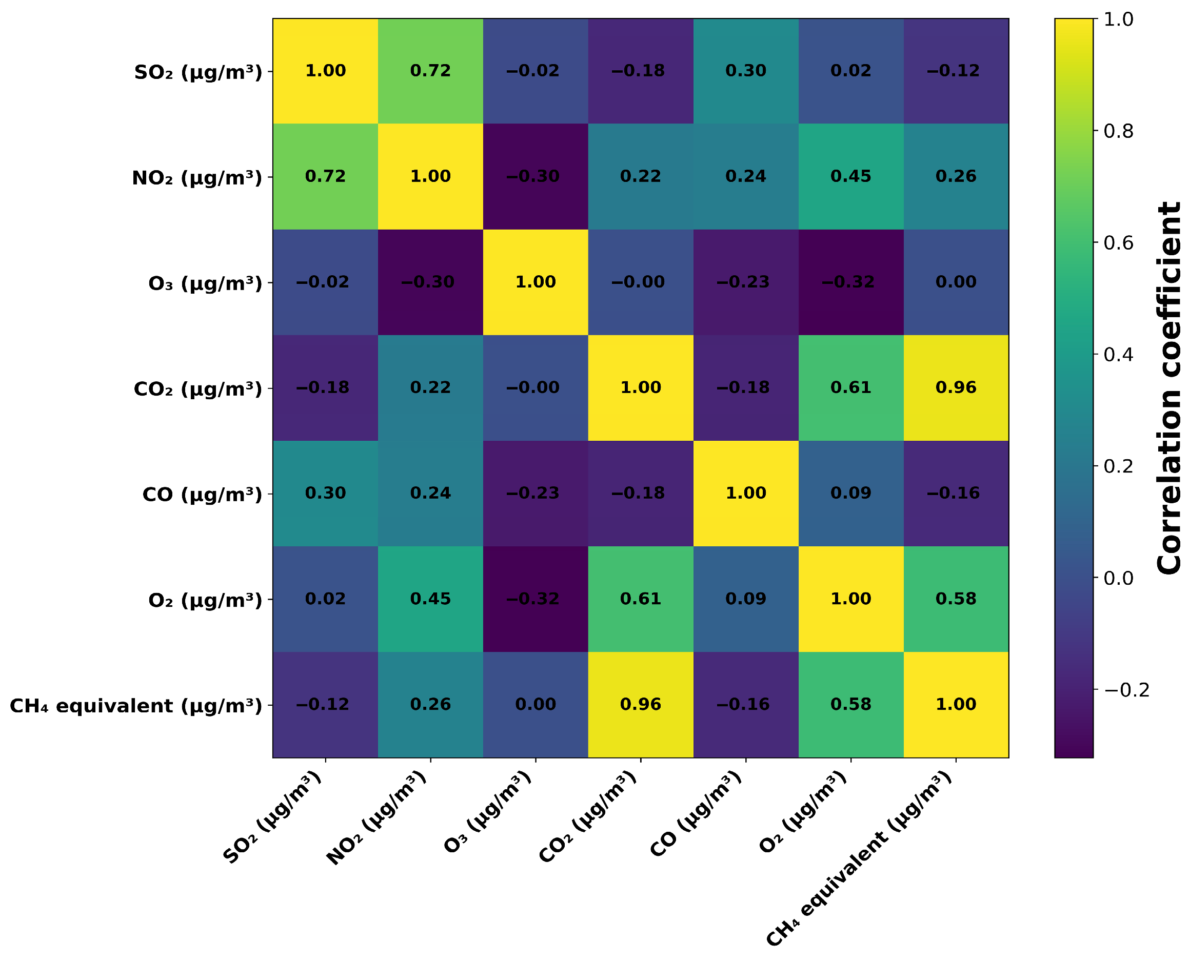
To enhance the visual interpretation derived from the individual time series and the z-score normalized representation, the statistical relationship between the monitored variables was evaluated using a correlation matrix. This analysis allowed for the identification of which gases exhibited opposite behaviors, which tended to vary in tandem, and which showed weak or nearly no connections during the monitoring period. The correlation heat map of the measured gas concentrations is displayed in Figure 5.
According to the data, the strongest positive correlation (r = 0.96) between CO2 and CH4 equivalent. This result supports their shared origin in landfill biogas produced during the anaerobic degradation of organic matter and is consistent with the patterns seen in the preceding subsections, where both variables increased around 13:10 h. Further positive correlations existed between SO2 and NO2 (r = 0.72), CO2 and O2 (r = 0.61), and O2 and CH4 equivalent (r = 0.58), indicating partially shared temporal responses during the monitoring period.
Conversely, the strongest negative correlation was found between O3 and O2 (r = −0.32) and between O3 and NO2 (r = −0.30). The inverse O3-NO2 relationship is consistent with its overall behavior in atmospheric photochemical processes, in which ozone formation and depletion are related to NOx chemistry. Although this relationship should be analyzed with caution, the negative trend between O2 and O3 could reflect the differences that exist between sectors that are impacted by atmospheric mixing and oxidation processes, as well as those who are most affected by landfill gas accumulation. In contrast, some correlations, such as those of SO2 and O3 (r = −0.02) and that of O3 and CH4 equivalent (r = 0.00), showed during the monitoring period a low or zero linear correlation.
Analyzing the concentration distribution of each gas over the monitoring period was as important as examining the statistical correlations between the variables. Box plots, which provide a visual depiction of the data’s dispersion, central tendency, and outlier occurrence, were used to accomplish this.

Distribution and Dispersion of Gas Concentrations

Box diagrams were used to examine the distribution of concentrations recorded for each gas in the scan intervals, as well as for sequential analysis and correlation assessment. This representation, which summarizes the general variability, interquartile range, median, and the existence of outliers, makes direct comparison feasible between gases with different concentration ranges. These graphs serve to distinguish the relatively stable concentration levels of intermittent events with high concentration, and also to separate the gases that appear to be most strongly influenced by local emission areas or spatial heterogeneity in the monitored area.
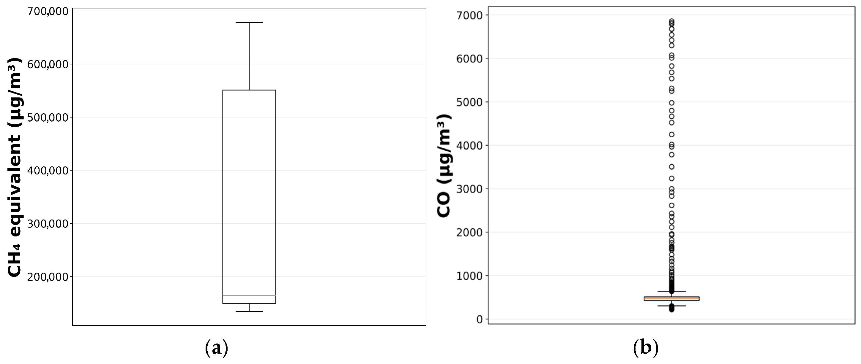
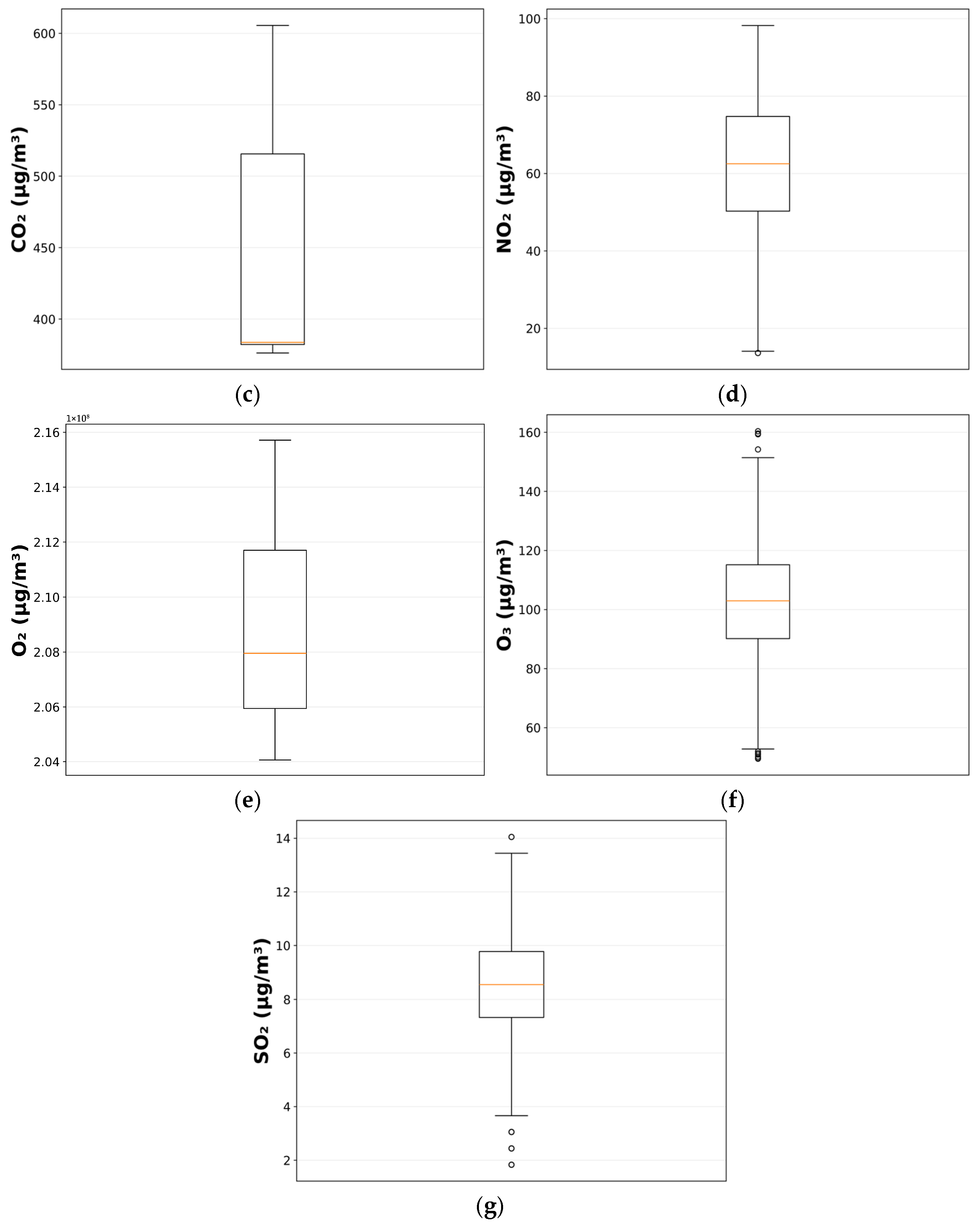
The box diagrams shown in Figure 6 made it easier to identify outliers in each monitored species and to compare the dispersion of concentrations. In general, this representation confirms that the gases did not exhibit uniform behavior throughout the survey but instead displayed varying levels of variability. This is consistent with the trends previously seen in sequential profiling and correlation analysis.
The CH4 equivalent and CO2 examples (Figure 6a–c) show broad distributions, with a large tail extending toward high values and medians pushed toward the lower end of the box. In the case of CO (Figure 6b), a different pattern emerges, in which a relatively compact box diagram matches a large number of high-magnitude outliers. This indicates that, although most of the CO observations remained within a relatively narrow range, occasional brief concentration peaks also occurred during the study. These extreme values, in the framework of landfill monitoring, may reflect transient localized events, such as the interception of feathers or combustion-related influences nearby, and therefore should not be interpreted solely as statistical anomalies.
On the other hand, the dispersion of NO2, O3, and SO2 shown in Figure 6d–g is moderate or intermediate. NO2 shows some odd low values, whereas O3 shows extreme observations at both the bottom and upper ends, suggesting a more variable signal. A few solitary events are also found outside of the center range, despite the fact that the distribution is more compact in the case of SO2. Ultimately, these variables show considerable variability, though not as much as individual CO events or the CH4 equivalent. The behavior of O2 depicted in Figure 6e also shows a significant amplitude in absolute terms, but it should be interpreted with caution due to its high atmospheric abundance compared to the other species. Nevertheless, the amplitude of the box and whiskers confirmed that this variable also underwent noticeable changes throughout the mission.
Overall, these box diagrams provide a pragmatic perspective on whether each gas was uniformly detected or not during the investigation. Thus, one can distinguish between relatively stable and more localized behavior, as well as between peaks and concentrated events that could be associated with heterogeneous landfill emissions.
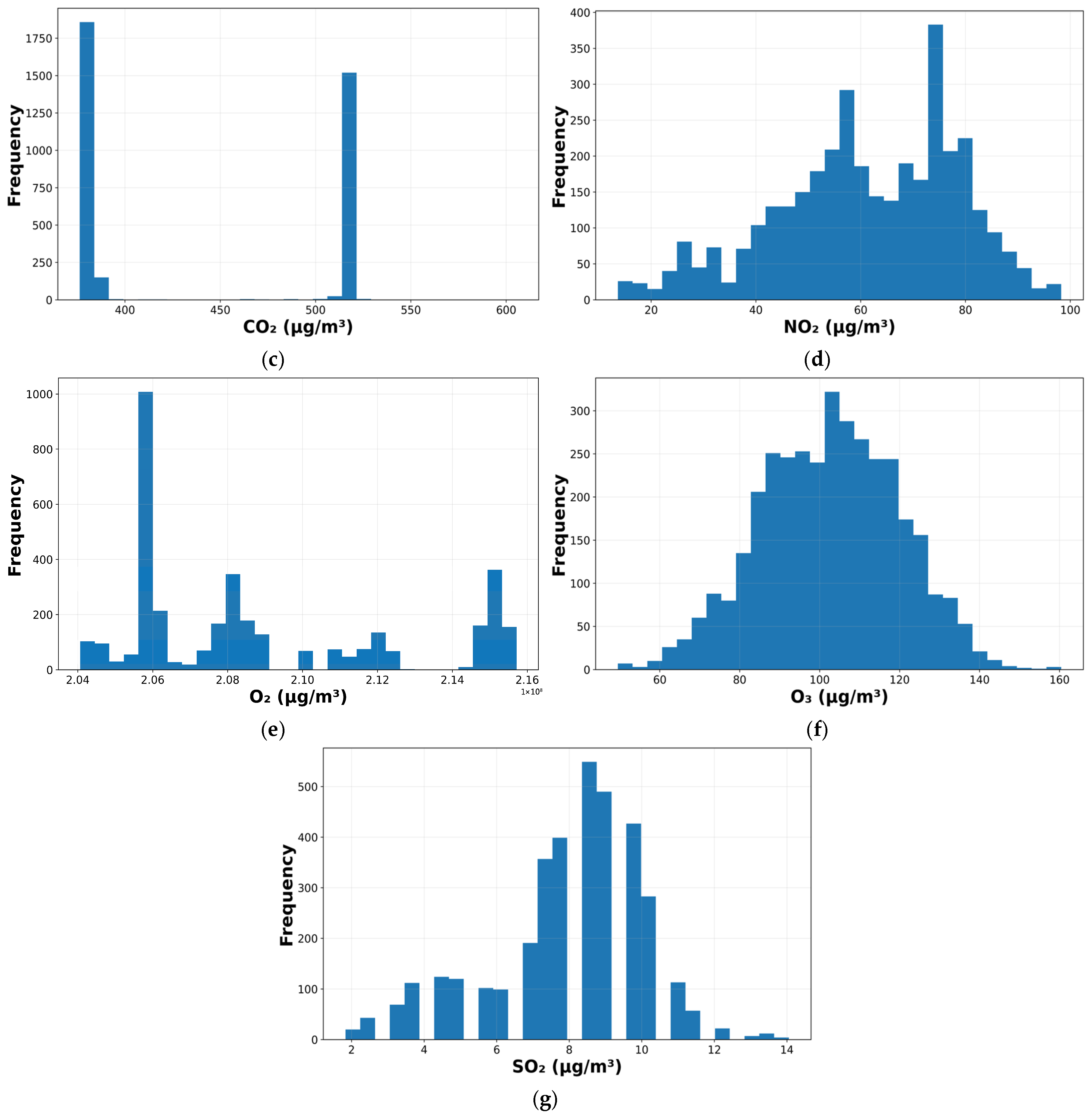
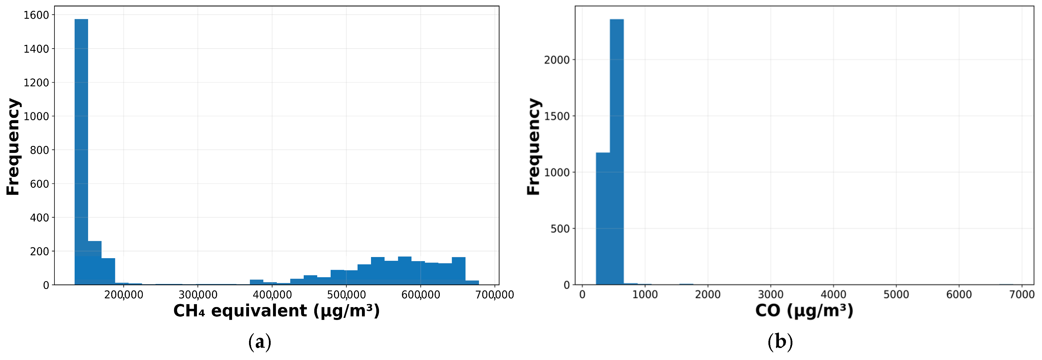
The histograms in Figure 7 provide an additional perspective on the concentration data. Histograms allow observation of the frequency with which different concentration ranges occurred throughout the survey, whereas box diagrams provide a synthesis of average value behavior, dispersion and out of the ordinary values. Thus, they help to establish whether the measures were grouped in a narrow range, in a broad spectrum, or if they were distributed over more than one characteristic concentration band. The histograms for CO2 and CH4 equivalent (in Figure 7a,c) do not have an easy concentration around a single main interval but rather show an accumulation of observations at multiple intervals. This pattern supports the idea that gas has a heterogeneous influence in spatial terms within the monitored area and is consistent with the existence of more than one concentration regime during monitoring.
In the case of CO (Figure 7b), most observations are concentrated at low values, and a smaller proportion is distributed to higher concentrations, producing a distribution with a very sharp right biased bias. This behavior is consistent with a background signal that is usually low, although it is interrupted by high concentration point events.
For NO2, O3 and SO2, the distributions are more continuous (see Figure 7d,f,g). O3 has an extensive distribution concentrated in intermediate values, indicating that it has a variable and not very grouped signal. NO2 has a wider concentration range, indicating greater variability during the study. On the other hand, SO2 is concentrated in a more limited range, which is consistent with its lower total dispersion. For O2 (Figure 7e), the observations are distributed among several concentration bands rather than concentrated in a single predominant peak, which again demonstrates that the monitored area did not present a homogeneous concentration field throughout the mission.
In this way, the histograms complement the evaluation of the box diagrams by representing the distribution of concentration frequencies throughout the survey. This helps to distinguish between gases that are dominated by narrow, low-level intervals and those affected by more extensive variability, multiple concentration regimes, or sporadic events with high concentrations.

3.3. Spatial Distribution Based on Interpolated Maps

The spatial distribution of the monitored gases within the research area was examined by creating interpolated maps using the standard kriging approach based on the georeferenced data gathered during the measurement surveys. These maps provide a continuous view of concentration fluctuations and facilitate the identification of areas with higher or lower concentrations of each gas. For ease of understanding, the data are presented in pairs of gases, which facilitates the comparison of their spatial patterns.
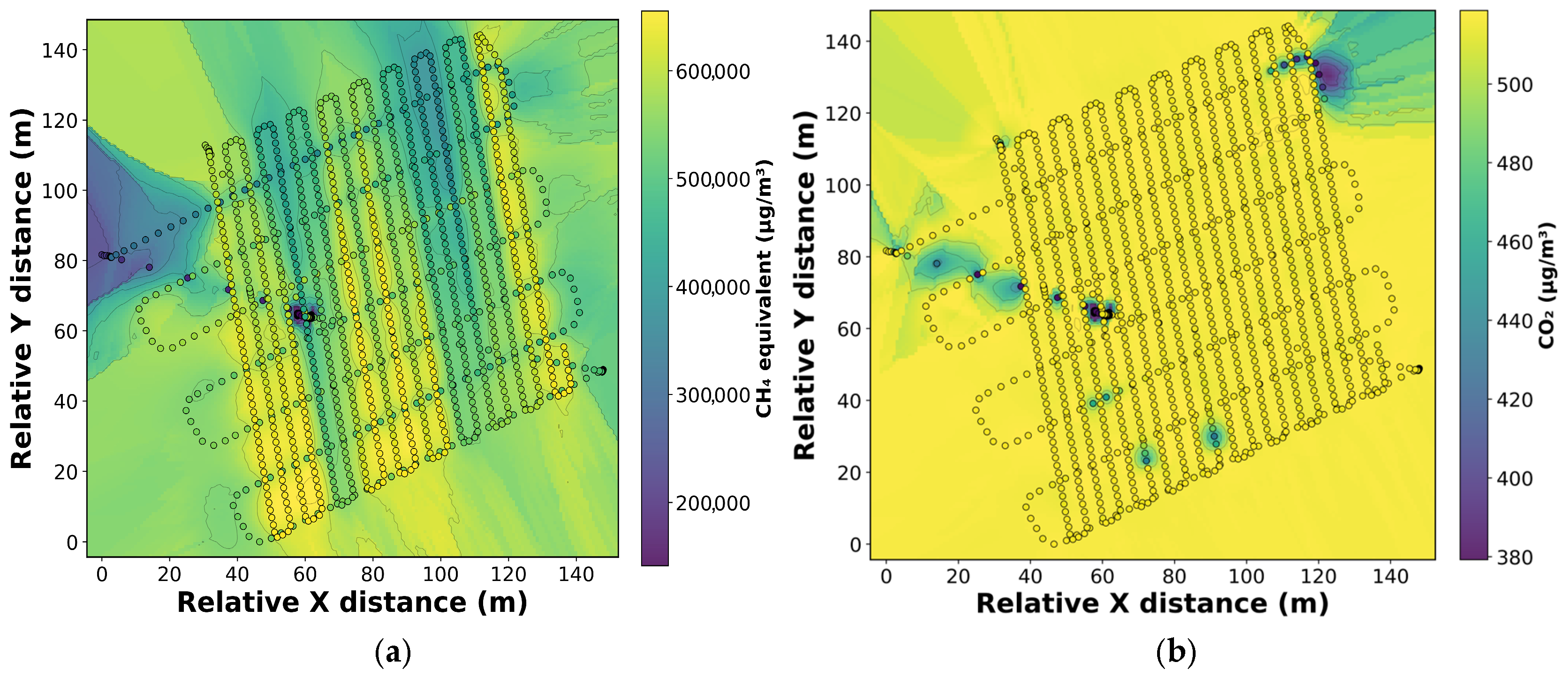
More noticeable geographic variability can be seen in Figure 8a, which displays the interpolated map of CH4 equivalent. Higher concentration bands are primarily found in the central, southern, and eastern regions of the monitored area. Conversely, a minor localized anomaly close to the route’s center and areas of lower concentration are found at the western end. Compared to CH4, the interpolated CO2 map in Figure 8b shows a more uniform distribution with relatively high and constant values across most of the studied area. Although there are some isolated areas of lower concentration, particularly in the western sector, at a central anomaly, and toward the northeastern boundary, the interpolated CO2 surface is generally more uniform and exhibits less abrupt spatial transitions.
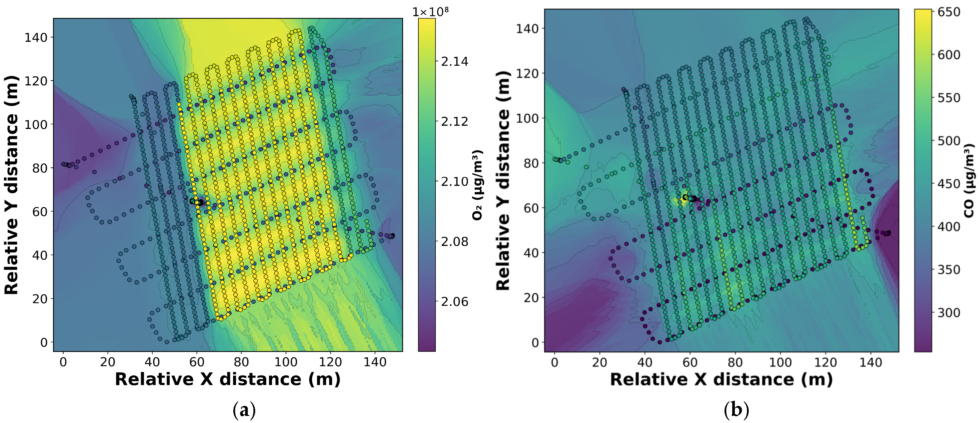
Continuing with the map interpolation, Figure 9a, which shows the interpolated O2 map, reveals a fairly wide distribution of high values in the middle of the monitored area, with lower concentrations near its eastern and western borders.
The interpolated CO map in Figure 9b is more varied than the O2 distribution. Higher-concentration anomalies are visible in the center region and in different parts of the eastern edge, particularly near the intersection of several sampling lines. Concurrently, the lowest concentrations are primarily found near the assessed region’s borders, particularly the southwest sector and the eastern boundary.
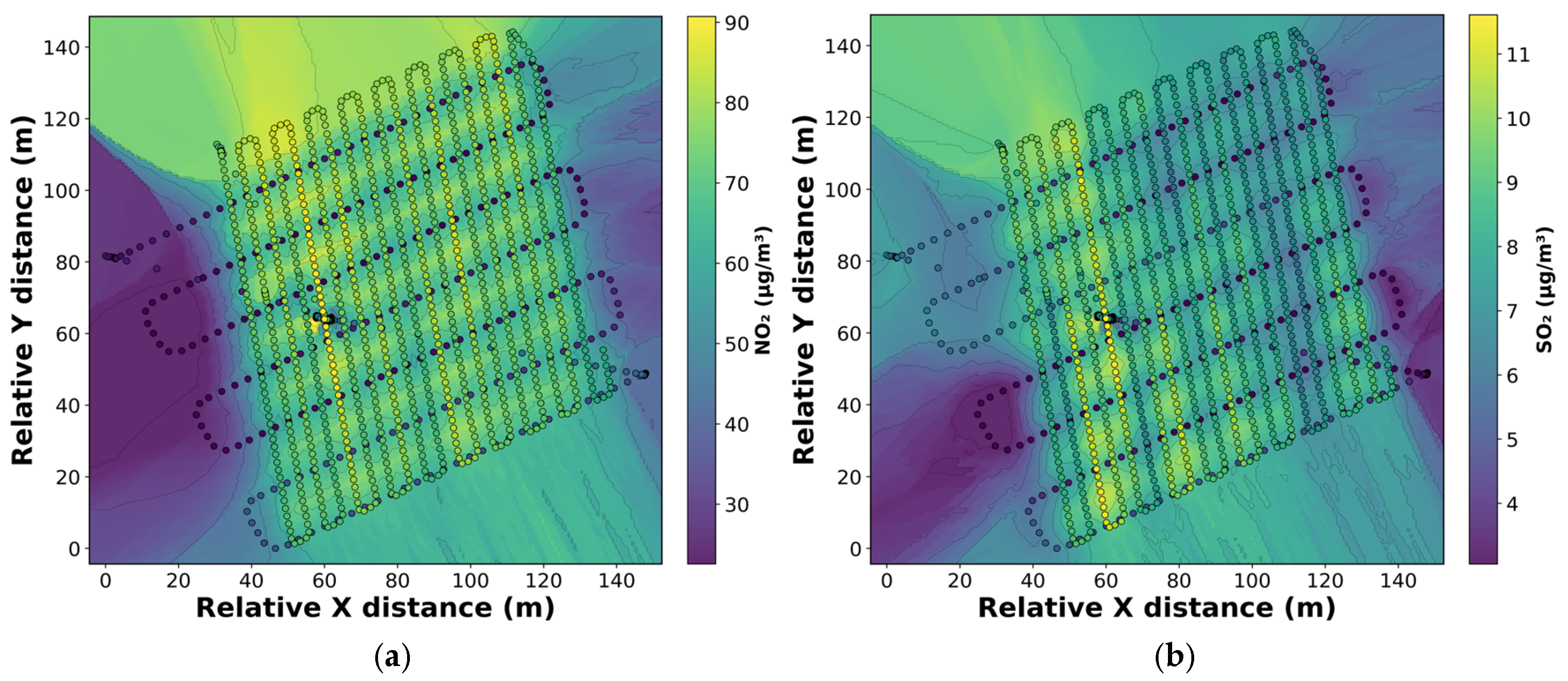
In contrast, the interpolated NO2 map in Figure 10a shows a relatively uniform spatial distribution within the main control region, with moderate to high concentrations predominating over a significant portion of the central area. The highest values tend to cluster in bands toward the central and north-central sectors, while the lowest concentrations are most clearly observed at the western and eastern boundaries of the assessed region.
Additionally, Figure 10b shows a more varied distribution of SO2, with more isolated anomalies and more noticeable spatial changes throughout the study area. In this case, the relatively higher concentrations are primarily found in bands in the middle and central-western sectors as well as in some parts of the southern zone, while the lowest values are found along the southwestern edge and in a section of the eastern boundary.
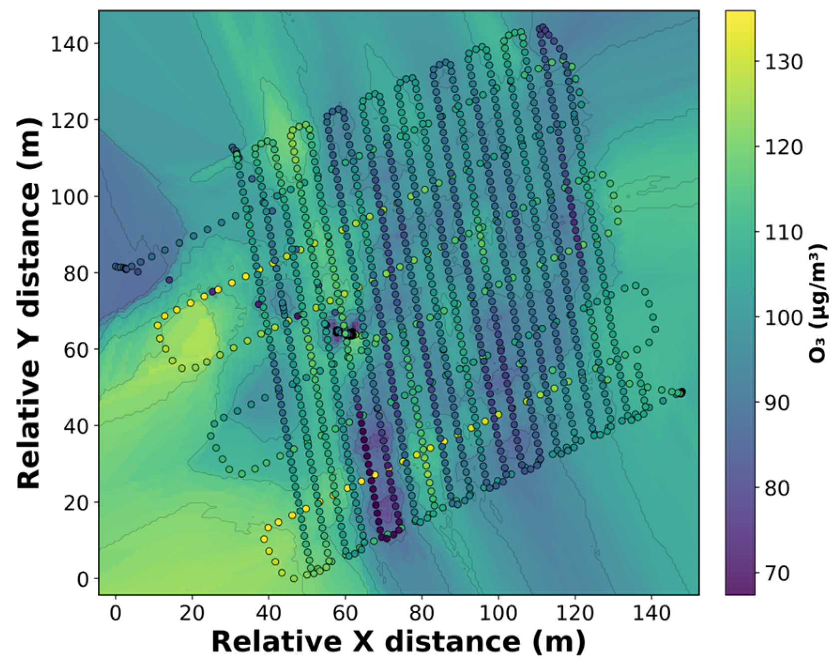
Finally, although it follows a different pattern than the preceding gases, the O3 distribution corresponding to the interpolated map in Figure 11 exhibits a heterogeneous spatial distribution. Comparatively higher concentrations are found in the western and northwestern sectors of the research area, as well as some remote areas in the southern sector. Conversely, bands of lower concentration are observed within the primary monitoring region, particularly in the central sector and the south-central zone.

3.4. Environmental Variables and Their Relationship to Gas Concentration

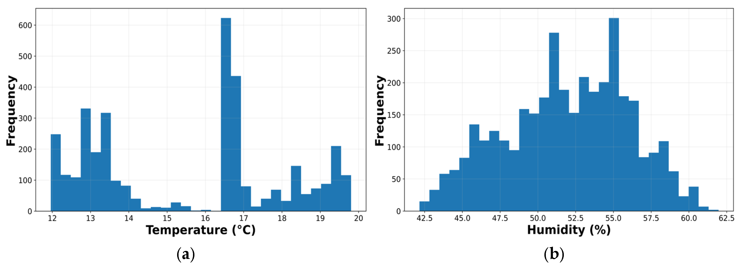
In this context, it is clear from the grouped histograms in Figure 12a,b that both variables displayed distinct ranges of fluctuation throughout the mission distinct ranges of fluctuation throughout the mission, the variables had different distributions. In terms of temperature (Figure 12a), the frequency of observations was dispersed across several ranges rather than concentrated in a single interval, suggesting fluctuations in temperature levels throughout the journey. Relative humidity, on the other hand, has a more continuous distribution (Figure 12b), mainly centered around middle values, but with sufficient amplitude to show environmental fluctuations specific to a site.
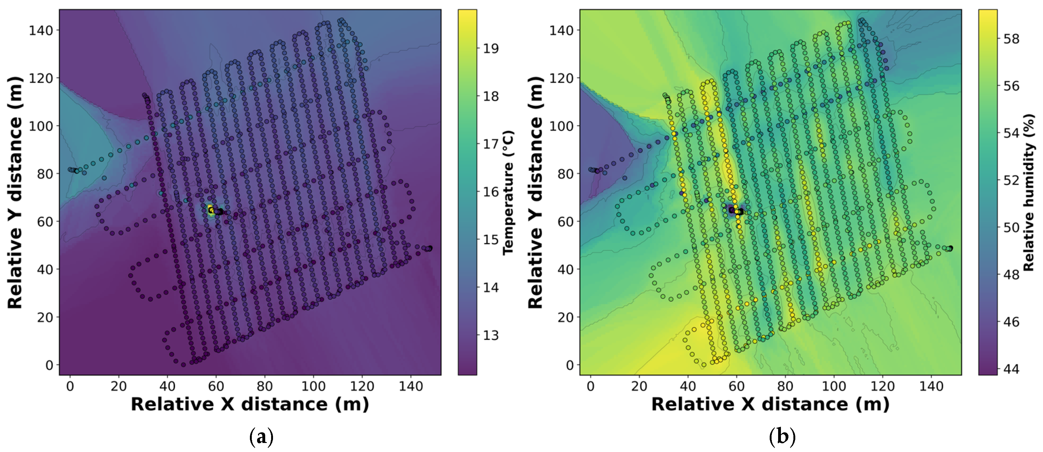
Temperature and relative humidity were not uniformly distributed throughout the study area, as shown by the interpolated maps in Figure 13a,b. Temperature (Figure 13a) shows localized areas with higher values, whereas relative humidity (Figure 13b) shows a varied spatial pattern with sectors where it tends to grow.
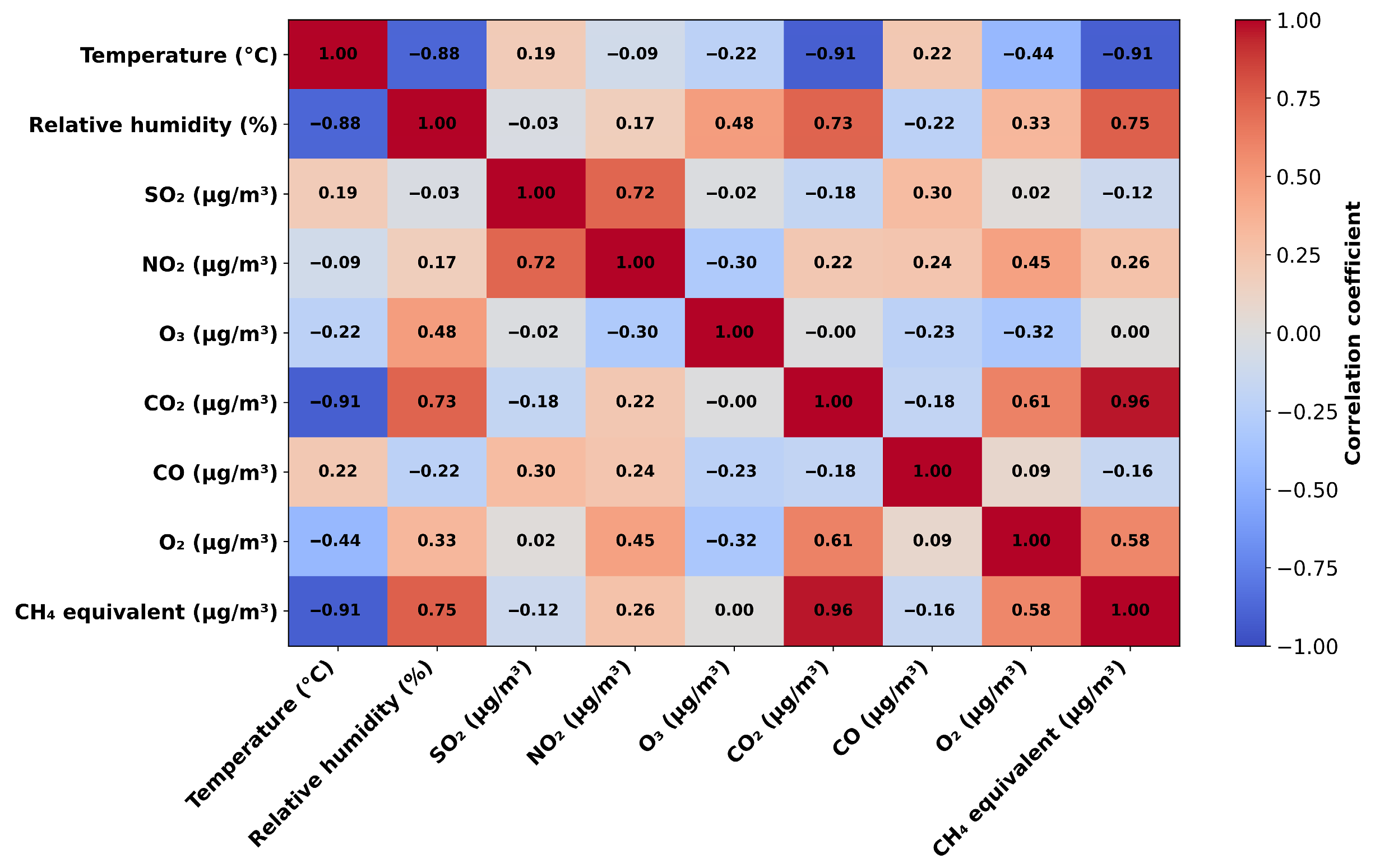
The correlation map, as shown in Figure 14, illustrates a more general view of the relationships between monitored gases and environmental variables. The most prominent inverse correlations were temperature with CO2 (r = −0.91) and the CH4 equivalent (r = −0.91). On the other hand, the two gases showed positive correlations with respect to relative humidity, r = 0.75 for CH4 and r = 0.73 for CO2. These patterns are consistent with the coupled behavior of the CH4 equivalent and CO2, which are the basic elements of landfill biogas; this indicates that higher concentrations tended to occur in colder, more humid local circumstances. These relationships may reflect microenvironmental differences in the monitored area, where conditions of higher humidity and lower temperature were simultaneously present, along with a less mixing or greater accumulation of gases, rather than indicating direct causality. For other species, the links with environmental variables were not so remarkable.

3.5. Spatial Analysis of the Thermal Orthophoto of the Study Area

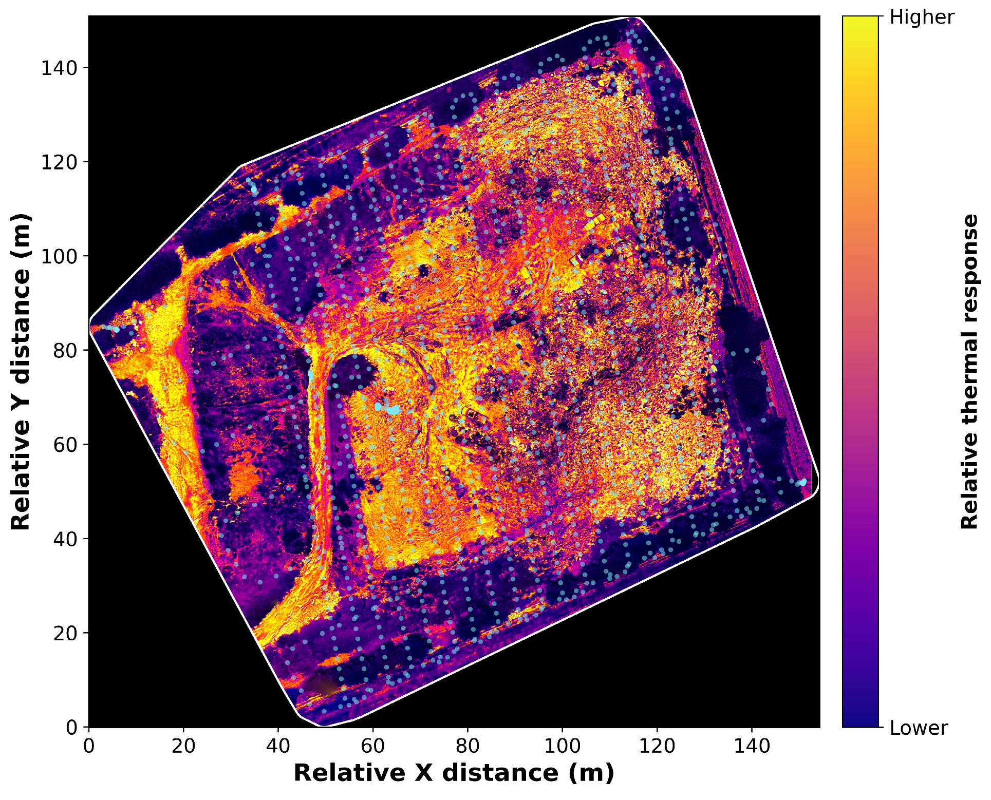
To complement the analysis of the interpolated gas maps, a thermal orthophoto of the monitored area was produced using photos taken during the flight and processed using WebODM with Python support for cartographic display. This output allows for the qualitative identification of areas with higher and lower thermal intensity inside the evaluated polygon because it displays a relative thermal response rather than absolute surface temperature data, unlike concentration maps.
Figure 15 shows that the heat response was not uniform across the entire research region. The areas with the highest thermal intensity, represented by colors of yellow and orange, are found in the central, central-eastern, and northern regions of the research area, along with a few linear features associated with highways or exposed surfaces. Conversely, the isolated sections and outer sectors of the site are the areas with the lowest thermal response, which are indicated by dark blue and purple hues. This pattern demonstrates the substantial spatial variation in the landfill’s surface thermal signature.
Although this product was not used to determine a direct quantitative correlation with the gas concentration maps, it enabled a qualitative analysis of spatial contrasts within the monitored area. As such, some sectors with different apparent thermal response also coincided with areas where changes in gas concentrations were recorded. This suggests that thermal orthophoto could be a valuable complementary layer for detecting areas of environmental interest.

4. Discussion

This sequence allowed us to relate temporal changes in air composition to their spatial expression within the landfill and to identify sectors potentially influenced by processes associated with biogas emissions.

4.1. Analysis of Temporal Behavior of Gas Concentration

Because each gas has its own concentration ranges and variation mechanisms, individual examination of the time series was necessary to identify emission patterns, local accumulation, and potential effects of atmospheric dispersion along the path. This tendency is interpreted as suggesting that the monitoring equipment passed through an area with higher methane concentrations or where atmospheric circumstances promoted local methane storage.
This suggests that CO was likely affected by a point source at the start or by transient conditions different from those governing methane behavior because it did not respond to the change observed halfway through the monitoring period in the same way.
The temporal congruence between the abrupt increase in CH4 equivalent and the virtually simultaneous change in behavior of both gases is particularly noteworthy. This lends credence to the theory that the system entered a region with a different gas composition or that site-associated emissions had a greater effect there. This may indicate that its concentration was more influenced by background sources outside the study location, atmospheric mixing processes, or local ventilation.
Although it may be anticipated that higher concentrations of gases associated with degradation processes would result in a more pronounced decrease in oxygen, this relationship does not manifest itself here in a clear-cut or instantaneous manner. This is explained by the great atmospheric abundance of O2 and the fact that its relative changes are far less obvious than those of other trace gases. This unpredictability was expected because ozone is a secondary pollutant whose dynamics are mostly dependent on photochemical reactions and air mixing conditions. As a result, its signal appears to respond more to the immediate air environment than to a limited direct emission.
This decline’s temporal congruence with the shift seen in other variables indicates that SO2 responded to the change in the measured air’s conditions, albeit at a relatively lower intensity.
When taken as a whole, the time series indicates that the mission underwent a significant turning point at around 13:10 h. At that moment, CO2 and CH4 equivalent drastically increased while NO2, O3, and SO2 significantly declined. The marked increase in CH4 and CO2 is attributed to the UAV intercepting a spatially confined region with a higher biogas influence. This behavior likely results from the combined effect of localized emission sources and atmospheric transport processes, such as plume advection or changes in mixing conditions within the lower boundary layer.

Integrated Interpretation of Temporal Variability in Gas Concentrations

The temporal coincidence between both variables, which suggests that the monitoring equipment reached an area with a different gas composition or with a stronger influence from local emissions, supports the previous conclusion based on the separate time series. This behavior shows that distinct atmospheric processes influenced separate variables instead of all responding in accordance with the same dynamics, which is the opposite of what was observed for CO2 and CH4 equivalent.
In general, it can be observed (see Figure 4) that at approximately 13:10 h, there was a substantial change in the composition of the analyzed air, as evidenced by the simultaneous, albeit divergent, reactions of the various gaseous species. However, a more fully integrated interpretation of the concentration transition around 13:10 h would also benefit from high-resolution meteorological measurements, especially wind speed and direction, that were not available for the current study and should be taken into account in future campaigns.

4.2. Interpretation of Statistical Relationships Between Gaseous Variables

Overall, the results indicate contradictory correlations between variables, indicating that the dynamics of the system were governed by a combination of emission processes, local accumulation, and atmospheric mixing rather than a single behavioral pattern.
These results demonstrate that while the reactions of the other species varied considerably, the dynamics of CO2 and CH4 equivalent were relatively comparable. This suggests that the composition of the air under observation was influenced by a number of variables rather than a single, reliable source. As a result, the correlation analysis provides a useful quantitative basis for verifying the presence of both similar and distinct behaviors among gases, thereby strengthening the comprehensive interpretation of the temporal data.

Interpretation of Gas Concentration Distribution and Dispersion

The regime change that was observed at around 13:10 h is consistent with this trend, which indicates a notable shift in concentration levels. Thus, the breadth of both distributions supports the hypothesis that at least two distinct air composition states coexisted during the monitoring period. This implies that even though most of the data were concentrated within a reasonable range, there were sporadic events with concentrations much higher than the core trend of the series. In this way, CO appears to have been dominated by short-lived events rather than a consistent increase throughout the study.
In general, the variables under observation displayed distinct dynamics: species such as NO2, O3, and SO2 exhibit more moderate fluctuations, albeit with sporadic deviations from the usual pattern, while CH4 equivalent and CO2 reflect well-defined regime shifts, CO stands out due to the presence of multiple outliers. These results complement the previous temporal study and provide a better picture of the dispersion and relative stability of each gas during the monitoring period.
This separation between the groups supports the hypothesis that both gases underwent a significant change in their concentration levels, which is consistent with the results of the time-series analysis. Consequently, the shape of the distribution lends credence to the idea that the overall behavior of CO was relatively stable, albeit punctuated by large-scale exceptional events.
This implies that the variable’s level fluctuated during the mission, but its interpretation, once more, needs to be done carefully because of the species’ characteristics within the atmospheric composition.
Finally, Figure 6a–g and Figure 7a–g show that the observed variables exhibited different distribution patterns. Species such as NO2, O3, and SO2 display more stable and moderate behavior, whereas CO2 and the CH4 equivalent show significant variations at different concentrations. The occurrence of sporadic extreme events makes CO unique. These statistical data support the interpretation presented in the previous subsections and confirm that the variability observed during the monitoring period was due to distinct dynamics among the gases.
In addition to the descriptive analysis of dispersion and distribution patterns, the observed behavior of certain gases can be interpreted in terms of their underlying generation and transformation mechanisms. In particular, the broad distributions observed for CH4 equivalent and CO2 are consistent with their strong positive correlation (r = 0.96), reflecting a common origin in landfill biogas production. Both gases are generated together during the anaerobic degradation of organic matter and typically dominate the landfill gas composition, which explains their coupled variability and the presence of high-concentration events associated with localized emission zones [31].
Conversely, the behavior of species such as O3, NO2, and SO2 appears to be governed not only by emission processes but also by atmospheric chemical transformations and transport. The variability and dispersion observed for O3, including the occurrence of extreme values, can be attributed to photochemical processes controlled by the NOₓ cycle and local atmospheric mixing. Under these conditions, inverse relationships between O3 and other gases such as NO2 can arise as a result of the equilibrium between ozone formation and depletion reactions in the lower atmosphere [32].
Overall, these patterns indicate that the statistical distributions presented in this section reflect a combination of variability derived from emissions and atmospheric processes, underscoring the need for an integrated interpretation when analyzing gas monitoring data obtained by unmanned aerial vehicles (UAVs).

4.3. Integrated Interpretation of Spatial Distribution Patterns

This pattern suggests that methane was not distributed uniformly throughout the site (see Figure 8), but rather exhibited a more localized distribution, most likely as a result of preferential emission points or differences in the intensity of the landfill’s decomposition processes. Increased atmospheric mixing and the fact that CO2 is affected by the background concentration of ambient air, in addition to its possible contribution from waste degradation, could be related to this behavior.
When the two maps are compared, the CH4 equivalent better revealed spatial variability within the monitored area, while CO2 showed a more diffuse and stable signal. Interestingly, some areas of lower concentration appear to coincide for both gases, particularly in the western sector and a small central region. This could be caused by local ventilation systems, atmospheric dilution, or a decreased direct impact from active emission sources.
Although kriging maps indicate that the high concentrations are not uniformly distributed, the flight path during this interval involved repeated passes over the same sector. Consequently, the persistence of elevated concentrations reflects not only the presence of emission hotspots but also the coupling between the UAV sampling strategy and the spatial heterogeneity of the gas field. This observation underscores a key limitation—and an opportunity—of UAV-based monitoring: sequential measurements inherently integrate spatial and temporal variability, requiring careful interpretation when reconstructing emission patterns in dynamic environments such as landfills.
This pattern indicated that oxygen had a moderate geographical variance and a more continuous signal within the primary sampling polygon. Combining the two images suggests that while O2 maintained a more continuous distribution within the site, CO displayed more distinct and confined spatial fluctuations (see Figure 9).
In the case of NO2, the pattern showed moderate variability, with a less fragmented distribution than other gases and a spatial gradient that decreases toward the site boundaries. However, in the case of SO2, the spatial pattern appears to be more concentrated, with more distinct areas of higher concentration (see Figure 10). A combination of these data reveals that, although the concentrations of both gases in the central area of the site are similar, NO2 exhibited a more widespread and continuous pattern, whereas SO2 made it easier to distinguish isolated areas of variation.
This pattern implies that ozone (O3) showed a more erratic distribution with more noticeable spatial changes, which may be related to local atmospheric transformation, mixing, and transport processes within the research area.
The spatial reconstruction assumes quasi-stationary conditions during each scan. However, temporal variability (e.g., due to wind fluctuations or transient emissions) can introduce uncertainty into the interpolated maps. Consequently, the results should be interpreted as an approximation of the spatial distribution under transient atmospheric conditions, rather than as a strictly static field.

4.4. Discussion of Environmental Influences on Gas Concentrations

In addition to the study of gaseous species, temperature and relative humidity were taken into consideration as supporting environmental variables since both could influence local dispersion and accumulation conditions within the monitored area. Their inclusion allowed for a more comprehensive interpretation of the patterns observed in the gases, particularly when significant statistical correlations and regime transitions were discovered.
This alteration in distribution indicates that there are microenvironments in the study area, which is key to understanding documented fluctuations in gas concentrations. These results (see Figure 12, Figure 13 and Figure 14) suggest, in general terms, that higher levels of CH4 equivalent and CO were associated with cooler temperatures and higher relative humidity during the study period. This pattern is consistent with to the coupled behavior of the two gases as essential components of landfill biogas and suggests that higher concentrations were related to local situations that could have favored gas accumulation or decreased dispersion. In this sense, temperature and relative humidity are better interpreted as associated environmental indicators of the monitored microenvironment than as direct short-term factors for gas generation.
Relative humidity showed a moderately strong correlation with O3 (r = 0.48), while temperature showed little correlation with SO2, NO2, O3, and CO (see Figure 14). This suggests that the effects of environmental factors were not the same for all species but were more apparent in those that also displayed shared temporal dynamics, as was the case with CO2 and CH4 equivalent.
The addition of temperature and relative humidity provides a useful environmental context for examining the temporal and spatial behavior of the observed gases. Although these relationships should be interpreted as associations rather than evidence of direct causation, the results suggest that the site’s microenvironmental conditions may have favored the local accumulation of particular species during the mission, suggesting that environmental variations are in fact important parameters when monitoring the spatial distribution of gases.

4.5. Interpretation of Thermal Spatial Patterns from the Orthophoto

Generally, variations in the terrain’s surface properties, such as the amount of solar exposure, the existence of exposed materials, surface moisture, vegetation cover, and the heterogeneity of the waste that has been deposited may be linked to the observed differences. In this respect, areas with lower thermal intensity may be affected by shade, moisture, or vegetation, whereas areas with higher thermal response may be linked to drier, more compacted surfaces or those with less coverage (see Figure 15). However, these contrasts should be understood as relative thermal patterns rather than as a precise measurement of absolute temperature because the orthophoto is qualitative in nature.
Thermal orthophotos offer a spatial perspective that can be complementary to gas monitoring, as they help detect areas at the site with differentiated surface behavior. The thermal product was used in the current research as a qualitative layer, not as a radiometrically calibrated temperature map; therefore, no direct quantitative correlation with gas concentrations was established. However, their comparison with interpolated gas maps indicates that apparent thermal contrasts may be useful for distinguishing areas of environmental interest and for interpreting spatial heterogeneity in the studied area.
Overall, the results indicate that the observed area showed significant spatial heterogeneity in terms of gas distribution and apparent thermal response of the surface. Differences in the spatial behavior of each gas could be determined thanks to interpolated maps, while qualitative thermal orthophoto corroborated the existence of zones with different thermal patterns. Although this comparison was qualitative, the joint interpretation of these geospatial products provided a broader environmental view of the landfill and may be useful to guide future studies that seek to examine possible relationships between thermal anomalies and localized gas emissions.

4.6. Limitations and Practical Implications

Although the ongoing research was primarily designed for spatial characterization, the system also demonstrates its ability to track time series through consecutive flights by the same predetermined route. This type of approach could help identify differences between monitoring timelines, areas where emission is recurrent, and short-term variations. However, this application remains largely limited. The resulting profiles include variability in time and space, since measurements are collected sequentially, not simultaneously across locations. Also, flight resistance, changing weather conditions and mission segmentation could have an impact on the level of comparability of repeated studies. Thus, the platform can be better understood as a versatile tool for conducting multiple space studies that have interpretative value in time terms, rather than as a replacement for continuous monitoring from fixed points.
The endurance and power supply of UAVs are another limitation. As the mission was forced to split into successive flights of about 15 min, the data set is not a strictly continuous record, but rather a series of scans that are segmented by time. Although the same acquisition protocol and route were maintained, this segmentation may affect the direct comparability of flight intervals, as short-term changes in atmospheric conditions or gas dispersion between successive missions are possible. Therefore, the data set must be understood as a collection of segments that are comparable but not exactly continuous enough to characterize spatially in an exploratory way; however, it requires caution when assessing time continuity at a small scale.

5. Conclusions

This work demonstrated the feasibility of using a UAV-based atmospheric monitoring system for the geographic characterization of gases associated with biogas emissions at a landfill. The integration of a multi-gas station with a thermal camera installed on a DJI Matrice 350 RTK platform allowed for the collection of georeferenced data with sufficient detail to investigate the temporal behavior, statistical correlations between variables, and spatial distribution patterns of the compounds under observation. The proposed methodology provides a flexible and useful alternative for environmental assessment of sites where traditional point monitoring is insufficient to capture local variability.
The results showed that the air’s composition was altered throughout the flight. There was a discernible change around 13:10 h that suggested arrival into a region with a different air composition and greater impact from nearby pollutants. At that moment, NO2, O3, and SO2 decreased while CH4 equivalent and CO2 increased concurrently. This observation was corroborated by the dataset’s greatest positive correlation between CO2 and CH4 equivalent (r = 0.96), which showed that both variables exhibited closely connected temporal dynamics throughout the campaign.
From a spatial perspective, the interpolated maps showed that while CH4 equivalent, CO, and SO2 displayed more varied patterns, CO2, O2, and NO2 tended to display relatively more continuous distributions within the monitored region. On the other hand, O3 displayed a more unpredictable spatial pattern consistent with the effects of local mixing, transport, and atmospheric transformation. Furthermore, as evidenced by positive correlations with relative humidity (r = 0.75 and r = 0.73, respectively) and negative correlations with temperature (r = −0.91), higher concentrations of CO2 and CH4 equivalent tended to be associated with higher relative humidity and lower temperatures.
Additionally, the qualitative thermal orthophoto confirmed that the landfill’s surface showed clear variations in relative temperature responsiveness rather than uniform conditions, particularly in the central, central-eastern, and northern regions of the site. Although it does not allow the inference of absolute temperatures or the development of a direct relationship with internal landfill processes on its own, this product offered helpful spatial context and supported the interpretation of surface heterogeneity seen in the gas maps. Thus, the combination of multi-gas monitoring, geostatistical interpolation, and qualitative aerial thermography can create a more complete picture of the environmental behavior of the evaluated area. Further work should include multi-temporal campaigns, additional meteorological controls, and thermal processing with radiometric calibration to strengthen the interpretation of emission dynamics and improve the site’s environmental diagnosis.

Author Contributions

Conceptualization, M.H.-C., G.L.-R. and D.A.F.-B.; methodology, J.F.E.-V., B.N.C.-S., M.H.-C. and J.D.R.-F.; software, J.F.E.-V., J.D.R.-F. and G.L.-R.; validation, J.F.E.-V., J.D.R.-F., M.H.-C., G.L.-R. and D.A.F.-B.; formal analysis, J.F.E.-V. and J.D.R.-F.; investigation, J.F.E.-V., J.D.R.-F., M.H.-C., G.L.-R. and D.A.F.-B.; resources, M.H.-C., G.L.-R. and D.A.F.-B.; data curation, J.F.E.-V., J.D.R.-F. and G.L.-R.; writing—original draft preparation, J.F.E.-V., J.D.R.-F., M.H.-C. and D.A.F.-B.; writing—review and editing, J.F.E.-V., M.H.-C. and D.A.F.-B.; visualization, J.F.E.-V., B.N.C.-S., M.H.-C. and J.D.R.-F.; supervision, M.H.-C. and D.A.F.-B.; project administration, D.A.F.-B.; funding acquisition, D.A.F.-B. All authors have read and agreed to the published version of the manuscript.

Funding

This research was supported by the Secretaría de Educación, Ciencia, Tecnología e Innovación (SECTEI) of CDMX through the Project SECTEI/083/2024, “Mapeo y cuantificación CH4, CO, CO2, NOx y SOx en suelo y aire de la CDMX como estrategia de mitigación de gases para la reducción de efectos del cambio climático”.

Institutional Review Board Statement

Not applicable.

Informed Consent Statement

Not applicable.

Data Availability Statement

Data presented in this study are available on request from the corresponding author.

Acknowledgments

The authors would like to thank the public institution that provided the facilities for conducting this study at the landfill, as well as for granting access to the monitoring site. The comments and suggestions by the reviewers are deeply appreciated. Additionally, Juan Francisco Escudero Villegas thanks SIP–IPN for the graduate scholarship granted through the Programa de Maestría en Ingeniería y Diseño de Sistemas Sostenibles at IPN.

Conflicts of Interest

The authors declare no conflicts of interest.

References

  1. Fosco, D.; Molfetta, M.D.; Renzulli, P.; Notarnicola, B.; Carella, C.; Fedele, G. Innovative Drone-Based Methodology for Quantifying Methane Emissions from Landfills. Waste Manag. 2025, 195, 79–91. [Google Scholar] [CrossRef]
  2. Fjelsted, L.; Christensen, A.G.; Larsen, J.E.; Kjeldsen, P.; Scheutz, C. Assessment of a Landfill Methane Emission Screening Method Using an Unmanned Aerial Vehicle Mounted Thermal Infrared Camera—A Field Study. Waste Manag. 2018, 87, 893–904. [Google Scholar] [CrossRef]
  3. Johnson, D.; Clark, N.; Heltzel, R.; Darzi, M.; Footer, T.L.; Herndon, S.; Thoma, E.D. Methane Emissions from Oil and Gas Production Sites and Their Storage Tanks in West Virginia. Atmos. Environ. X 2022, 16, 100193. [Google Scholar] [CrossRef] [PubMed]
  4. Alvear, O.; Zema, N.R.; Natalizio, E.; Calafate, C.T. Using UAV-Based Systems to Monitor Air Pollution in Areas with Poor Accessibility. J. Adv. Transp. 2017, 2017, 8204353. [Google Scholar] [CrossRef]
  5. Villa, T.; Gonzalez, F.; Miljievic, B.; Ristovski, Z.; Morawska, L. An Overview of Small Unmanned Aerial Vehicles for Air Quality Measurements: Present Applications and Future Prospectives. Sensors 2016, 16, 1072. [Google Scholar] [CrossRef] [PubMed]
  6. Burgués, J.; Marco, S. Environmental Chemical Sensing Using Small Drones: A Review. Sci. Total Environ. 2020, 748, 141172. [Google Scholar] [CrossRef]
  7. Berman, E.S.F.; Fladeland, M.; Liem, J.; Kolyer, R.; Gupta, M. Greenhouse Gas Analyzer for Measurements of Carbon Dioxide, Methane, and Water Vapor Aboard an Unmanned Aerial Vehicle. Sens. Actuators B Chem. 2012, 169, 128–135. [Google Scholar] [CrossRef]
  8. Greatwood, C.; Richardson, T.; Freer, J.; Thomas, R.; MacKenzie, A.; Brownlow, R.; Lowry, D.; Fisher, R.; Nisbet, E. Atmospheric Sampling on Ascension Island Using Multirotor UAVs. Sensors 2017, 17, 1189. [Google Scholar] [CrossRef]
  9. Chang, C.-C.; Chang, C.-C.; Wang, J.-L.; Chang, C.-Y.; Chang, C.-Y.; Liang, M.-C.; Lin, M.-R. Development of a Multicopter-Carried Whole Air Sampling Apparatus and Its Applications in Environmental Studies. Chemosphere 2015, 144, 484–492. [Google Scholar] [CrossRef]
  10. Allen, G.; Hollingsworth, P.; Kabbabe, K.; Pitt, J.R.; Mead, M.I.; Illingworth, S.; Roberts, G.; Bourn, M.; Shallcross, D.E.; Percival, C.J. The Development and Trial of an Unmanned Aerial System for the Measurement of Methane Flux from Landfill and Greenhouse Gas Emission Hotspots. Waste Manag. 2018, 87, 883–892. [Google Scholar] [CrossRef]
  11. Fosco, D.; De Molfetta, M.; Renzulli, P.; Notarnicola, B. Progress in Monitoring Methane Emissions from Landfills Using Drones: An Overview of the Last Ten Years. Sci. Total Environ. 2024, 945, 173981. [Google Scholar] [CrossRef]
  12. Tanda, G.; Balsi, M.; Fallavollita, P.; Chiarabini, V. A UAV-Based Thermal-Imaging Approach for the Monitoring of Urban Landfills. Inventions 2020, 5, 55. [Google Scholar] [CrossRef]
  13. Bailey, S.C.C.; Sama, M.P.; Canter, C.A.; Pampolini, L.F.; Lippay, Z.S.; Schuyler, T.J.; Hamilton, J.D.; MacPhee, S.B.; Rowe, I.S.; Sanders, C.D.; et al. University of Kentucky Measurements of Wind, Temperature, Pressure and Humidity in Support of LAPSE-RATE Using Multisite Fixed-Wing and Rotorcraft Unmanned Aerial Systems. Earth Syst. Sci. Data 2020, 12, 1759–1773. [Google Scholar] [CrossRef]
  14. De Boer, G.; Palo, S.; Argrow, B.; LoDolce, G.; Mack, J.; Gao, R.-S.; Telg, H.; Trussel, C.; Fromm, J.; Long, C.N.; et al. The Pilatus Unmanned Aircraft System for Lower Atmospheric Research. Atmos. Meas. Tech. 2016, 9, 1845–1857. [Google Scholar] [CrossRef]
  15. Gaceta del Gobierno Del Estado de México. Decreto 293 por el que se autoriza el convenio de asociación municipal para la operación de un relleno sanitario regional y se aprueba la creación de un organismo público descentralizado encargado de su operación. Gaceta del Gobierno: Periódico Oficial del Gobierno del Estado Libre y Soberano de México. 2009, No. 29, 10 August. Available online: https://legislacion.edomex.gob.mx/sites/legislacion.edomex.gob.mx/files/files/pdf/gct/2009/ago105.PDF (accessed on 2 March 2026).
  16. Espejel, R. Juchitepec Cuenta Con Un Relleno Sanitario de Primer Nivel: Mejía—El Valle. Available online: https://elvalle.com.mx/2020/01/30/juchitepec-cuenta-con-un-relleno-sanitario-de-primer-nivel-mejia/ (accessed on 2 March 2026).
  17. Secretaría de Medio Ambiente y Recursos Naturales; Trujillo Segura, J.C.J.; Ortiz Conde, R.; Medina Arévalo, A.; Acevedo Portilla, L.F.; Navarro Reynoso, J.E.; Alcantar López, G.; Mendoza Aguirre, S.I.; Trigueros Esquiliano, R.; Díaz Ortiz, M.; et al. Diagnóstico Básico Para La Gestión Integral de Los Residuos, 1st ed.; SEMARNAT: Mexico City, Mexico, 2020. [Google Scholar]
  18. Emran, B.; Tannant, D.; Najjaran, H. Low-Altitude Aerial Methane Concentration Mapping. Remote Sens. 2017, 9, 823. [Google Scholar] [CrossRef]
  19. Baiocchi, V.; Napoleoni, Q.; Tesei, M.; Servodio, G.; Alicandro, M.; Costantino, D. UAV for Monitoring the Settlement of a Landfill. Eur. J. Remote Sens. 2019, 52, 41–52. [Google Scholar] [CrossRef]
  20. Khan, A.; Schaefer, D.; Tao, L.; Miller, D.J.; Sun, K.; Zondlo, M.A.; Harrison, W.A.; Roscoe, B.; Lary, D.J. Low Power Greenhouse Gas Sensors for Unmanned Aerial Vehicles. Remote Sens. 2012, 4, 1355–1368. [Google Scholar] [CrossRef]
  21. De Sousa Mello, C.C.; Salim, D.H.C.; Simões, G.F. UAV-Based Landfill Operation Monitoring: A Year of Volume and Topographic Measurements. Waste Manag. 2021, 137, 253–263. [Google Scholar] [CrossRef]
  22. Alejo-Sanchez, L.E.; Márquez-Grajales, A.; Salas-Martínez, F.; Franco-Arcega, A.; López-Morales, V.; Acevedo-Sandoval, O.A.; González-Ramírez, C.A.; Villegas-Vega, R. Missing Data Imputation of Climate Time Series: A Review. MethodsX 2025, 15, 103455. [Google Scholar] [CrossRef] [PubMed]
  23. AlSalehy, A.S.; Bailey, M. Improving Time Series Data Quality: Identifying Outliers and Handling Missing Values in a Multilocation Gas and Weather Dataset. Smart Cities 2025, 8, 82. [Google Scholar] [CrossRef]
  24. Oliver, M.A.; Webster, R. A Tutorial Guide to Geostatistics: Computing and Modelling Variograms and Kriging. CATENA 2013, 113, 56–69. [Google Scholar] [CrossRef]
  25. Munyati, C.; Sinthumule, N.I. Comparative Suitability of Ordinary Kriging and Inverse Distance Weighted Interpolation for Indicating Intactness Gradients on Threatened Savannah Woodland and Forest Stands. Environ. Sustain. Indic. 2021, 12, 100151. [Google Scholar] [CrossRef]
  26. Alsamamra, H.; Ruiz-Arias, J.A.; Pozo-Vázquez, D.; Tovar-Pescador, J. A Comparative Study of Ordinary and Residual Kriging Techniques for Mapping Global Solar Radiation over Southern Spain. Agric. For. Meteorol. 2009, 149, 1343–1357. [Google Scholar] [CrossRef]
  27. Sledz, A.; Unger, J.; Heipke, C. Thermal Ir Imaging: Image Quality and Orthophoto Generation. Int. Arch. Photogramm. Remote Sens. Spatial Inf. Sci. 2018, XLII-1, 413–420. [Google Scholar] [CrossRef]
  28. Kelly, J.; Kljun, N.; Olsson, P.-O.; Mihai, L.; Liljeblad, B.; Weslien, P.; Klemedtsson, L.; Eklundh, L. Challenges and Best Practices for Deriving Temperature Data from an Uncalibrated UAV Thermal Infrared Camera. Remote Sens. 2019, 11, 567. [Google Scholar] [CrossRef]
  29. Kostrzewa, A.; Płatek-Żak, A.; Banat, P.; Wilk, Ł. Open-Source vs. Commercial Photogrammetry: Comparing Accuracy and Efficiency of OpenDroneMap and Agisoft Metashape. In The International Archives of the Photogrammetry, Remote Sensing and Spatial Information Sciences/International Archives of the Photogrammetry, Remote Sensing and Spatial Information Sciences; Copernicus GmbH: Göttingen, Germany, 2025; Volume XLVIII-1/W4-2025, pp. 65–72. [Google Scholar] [CrossRef]
  30. Brovkina, O.; Fajmon, L.; Pikl, M.; Zemek, F. Application of UAV Orthophoto and Thermal Imaging for Municipal Solid Waste Landfills Monitoring. In ISPRS Annals Of The Photogrammetry, Remote Sensing And Spatial Information Sciences; Copernicus GmbH: Göttingen, Germany, 2025; Volume X-2/W2-2025, pp. 1–6. [Google Scholar] [CrossRef]
  31. Kjeldsen, P.; Barlaz, M.A.; Rooker, A.P.; Baun, A.; Ledin, A.; Christensen, T.H. Present and Long-Term Composition of MSW Landfill Leachate: A Review. Crit. Rev. Environ. Sci. Technol. 2002, 32, 297–336. [Google Scholar] [CrossRef]
  32. Han, S.; Bian, H.; Feng, Y.; Liu, A.; Li, X.; Zeng, F.; Zhang, X. Analysis of the Relationship between O3, NO and NO2 in Tianjin, China. Aerosol Air Qual. Res. 2011, 11, 128–139. [Google Scholar] [CrossRef]
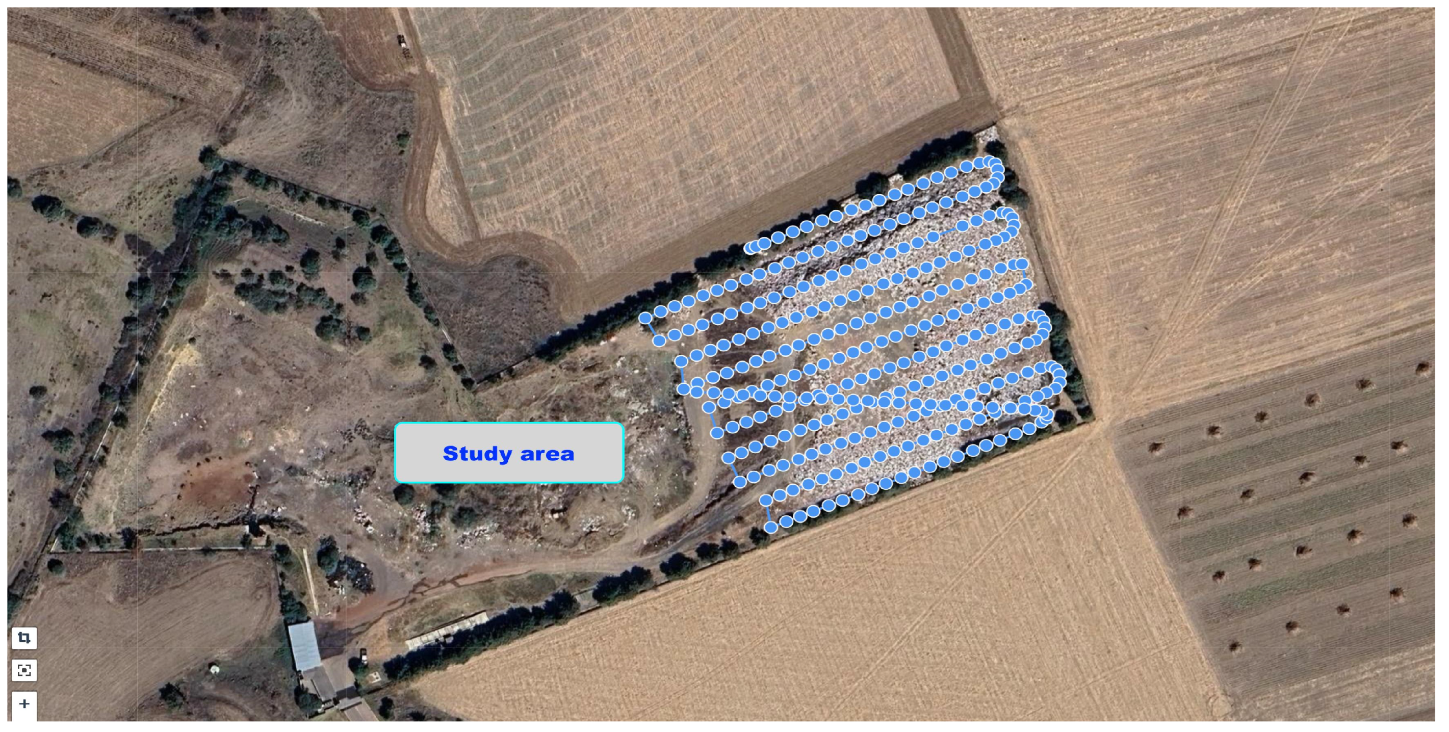
Figure 1. Aerial view of the study site. The blue dots indicate the route taken to collect data using a UAV.
Applsci 16 03970 g001
Figure 2. UAV trajectory during the monitoring mission, showing the flight segment related to the concentration transition observed around ~13:10 h. The green star indicates the starting point of the flight, while the blue circles represent the full UAV trajectory path.
Applsci 16 03970 g002
Figure 3. Sequential gas concentration measurements acquired along the UAV flight path during the monitoring mission for: (a) CH4; (b) CO; (c) CO2; (d) NO2; (e) O2; (f) O3; (g) SO2.
Applsci 16 03970 g003aApplsci 16 03970 g003b
Figure 4. Z-score normalized time series for comparing trends among the monitored gases.
Applsci 16 03970 g004
Figure 5. Heat map of the correlation matrix between the concentrations of the gases monitored during the mission.
Applsci 16 03970 g005
Figure 6. Box plots of the recorded concentrations for: (a) CH4 equivalent; (b) CO; (c) CO2; (d) NO2; (e) O2; (f) O3; (g) SO2 used to compare the dispersion, the central tendency of the data, and the presence of outliers during the monitoring mission. The orange line within each box represents the median value.
Applsci 16 03970 g006aApplsci 16 03970 g006b
Figure 7. Histograms of the recorded concentrations for: (a) CH4 equivalent; (b) CO; (c) CO2; (d) NO2; (e) O2; (f) O3; (g) SO2, used to illustrate the frequency distribution and the predominant concentration ranges during the monitoring mission.
Applsci 16 03970 g007aApplsci 16 03970 g007b
Figure 8. Maps interpolated using ordinary kriging of: (a) CH4 equivalent; (b) CO2 in the study area. CH4 equivalent exhibited greater spatial heterogeneity, while CO2 showed a relatively more uniform distribution. The circles represent the sampling points acquired along the UAV flight trajectory used for the interpolation.
Applsci 16 03970 g008
Figure 9. Maps interpolated using ordinary kriging for: (a) O2; (b) CO in the study area. O2 exhibited a relatively more continuous distribution in the central zone, while CO showed greater spatial heterogeneity with localized anomalies. The circles indicate the measurement points collected along the UAV flight path used for the interpolation.
Applsci 16 03970 g009
Figure 10. Maps interpolated using ordinary kriging for: (a) NO2; (b) SO2 in the study area. NO2 exhibited a relatively more continuous distribution in the central zone, while SO2 showed a more heterogeneous pattern, with localized anomalies in the central sector. The circles denote the data acquisition points along the UAV flight trajectory used for the interpolation.
Applsci 16 03970 g010
Figure 11. Map of O3 concentrations in the study area, interpolated using ordinary kriging. The circles correspond to the measurement points collected along the UAV flight path used for the interpolation.
Applsci 16 03970 g011
Figure 12. Histograms of: (a) temperature; (b) relative humidity, used to visualize the frequency distribution of environmental variables during the monitoring mission.
Applsci 16 03970 g012
Figure 13. Ordinary kriging interpolation map of environmental variables: (a) temperature, (b) relative humidity, measured at the study site. The circles correspond to the measurement points collected along the UAV flight path used for the interpolation.
Applsci 16 03970 g013
Figure 14. Heat map of the correlation matrix between environmental variables and monitored gas concentrations, used to identify positive, negative, and weak associations between variables.
Applsci 16 03970 g014
Figure 15. Qualitative thermal orthophoto of the monitored area at the landfill. The color scale represents the relative thermal response of the surface, ranging from areas of lower to higher apparent thermal intensity, without indicating absolute temperature values. Blue points correspond to the spatial distribution of image acquisition used in the generation of the thermal orthomosaic.
Applsci 16 03970 g015
Table 1. Features and specifications of the UAV platform.
Specifications
UAV platformDJI Matrice 350 RTK
Weight 6.47 kg
Dimensions810 mm × 670 mm × 430 mm
Autonomy55 min
Speed 23 m/s
GNSSGPS + Galileo + BeiDou + GLONASS
Table 2. Technical specifications of the gas monitoring system.
ParameterDetection MethodRange
CxHy/CH4/LELnon-dispersive infrared (NDIR)0~5% VOL (0~100% LEL) methane,
or 0~2% VOL propane
CO2non-dispersive infrared (NDIR)50,000 ppm
COelectrochemistry0~1000 ppm
NO2electrochemistry0~11 ppm
O3 + NO2electrochemistry0~11 ppm
SO2electrochemistry0~100 ppm
O2electrochemistry0–50%
Table 3. UAV flight configuration.
ParameterConfigured ValueDescription
Flight altitude20 m AGLThis altitude maximizes thermal resolution without compromising operational safety or the aerodynamic stability of the UAV.
Flight speed14 m/sThis speed allowed the mission to be completed within the UAV’s battery limits while maintaining adequate image overlap for subsequent thermal processing.
Camera angle90° (nadir)Automatically adjusted in ortho-collection mode, ensuring geometric uniformity, reduces angular variability, and improves photogrammetric reconstruction efficiency.
Disclaimer/Publisher’s Note: The statements, opinions and data contained in all publications are solely those of the individual author(s) and contributor(s) and not of MDPI and/or the editor(s). MDPI and/or the editor(s) disclaim responsibility for any injury to people or property resulting from any ideas, methods, instructions or products referred to in the content.