Extraction of Stone Positions from a Sheet Image for Curling Match Database Construction

Abstract

Curling is a sport in which two teams take turns delivering stones on ice and compete for total scores. It is a highly strategic sport, often referred to as “Chess on Ice”. In recent years, research on curling AI and statistical analysis aimed at tactical evaluation has been active. Decision-making in curling highly depends on the current stone position state, so obtaining stone positions is essential for tactical analysis. This study proposes an object detection model capable of acquiring stone coordinates with high accuracy and generality from stone position images of actual games. The proposed model was realized with a small amount of manually annotated data and pseudo-labeled images. Using the active testing method, the image-level accuracy of data—a strict criterion requiring perfect detection of all stones in a single image—for approximately 100,000 items was estimated to be 99.37%. Furthermore, we measured the positional error of the detected stones and found an average result of 0.472 px. We determined that this model had sufficient accuracy for practical use, so we decided to store the acquired coordinates in a database and use them as training data for the curling AI and statistical analysis.

1. Introduction

Curling is a sport played on ice, in which two teams take turns delivering stones and compete for total scores accumulated over 8 or 10 units of play, called ends. Each team delivers 8 stones per end, a total of 16 stones, and the score is determined by the positions of the stones after all deliveries. Due to its highly strategic nature, in which scoring depends on the positioning of the stones, it is referred to as “Chess on Ice,” and the research and development of curling AI to support tactical analysis and evaluation has been promoted [1,2,3,4].

Accurate tracking of game situations is essential for computational analysis. In curling, each game situation can be identified using four hierarchical levels of information: game information, end state, shot information, and stone positions. The game information identifies a specific match, whereas the end state describes the static state of a particular end within that match, such as the end number, score difference, and which team delivers first. Given the match and end specified by the game information and end state, the shot information and stone positions identify a specific shot among the 16 shots delivered in that end and the resulting stone positions, respectively.

The information of stone positions, in particular, plays a critical role in strategic evaluation and decision-making. There are countless possible stone configurations, and even slight changes in stone positions can lead to different shot selections.

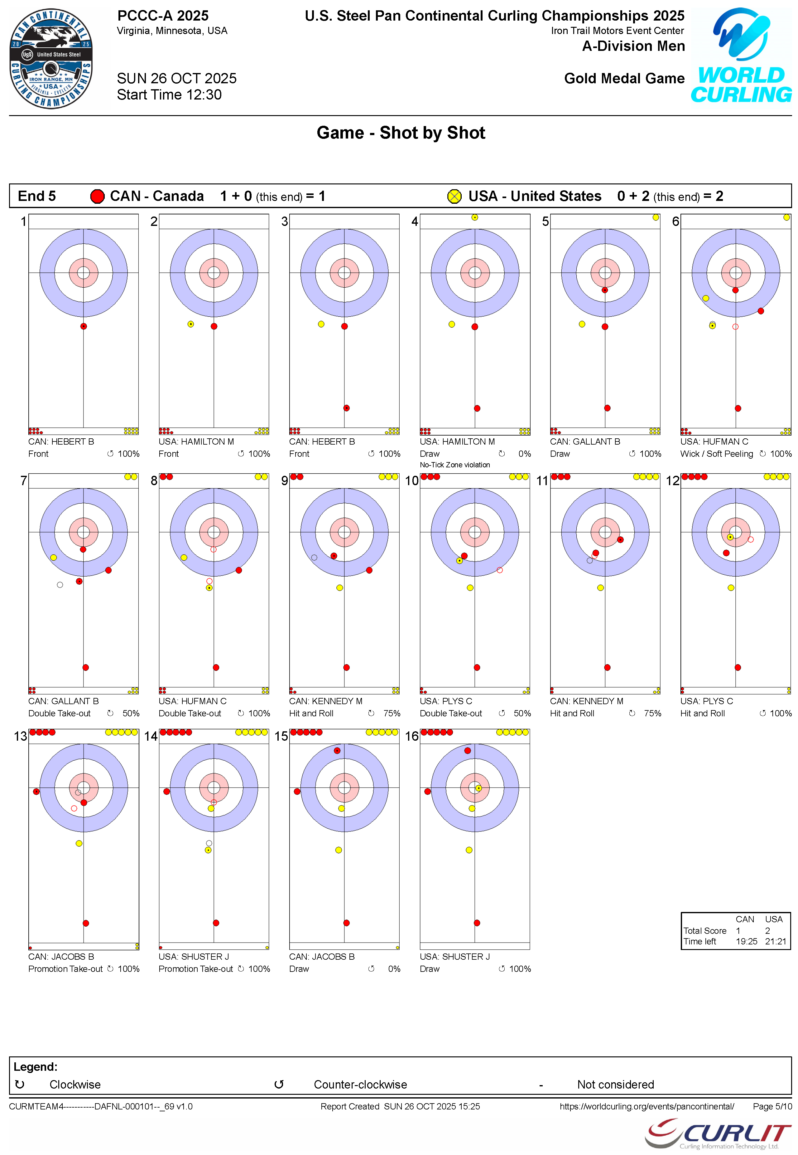
A comprehensive record of curling match logs is available in the Results Book [5] provided by CURLIT, which contains all of the aforementioned information for top-level competitions such as the European Championships, World Championships, and the Olympic Games. The Results Book is published in PDF format, in which the game information, end state, and shot information are provided as text, whereas the stone positions are displayed as images for each shot, as shown in Figure 1.

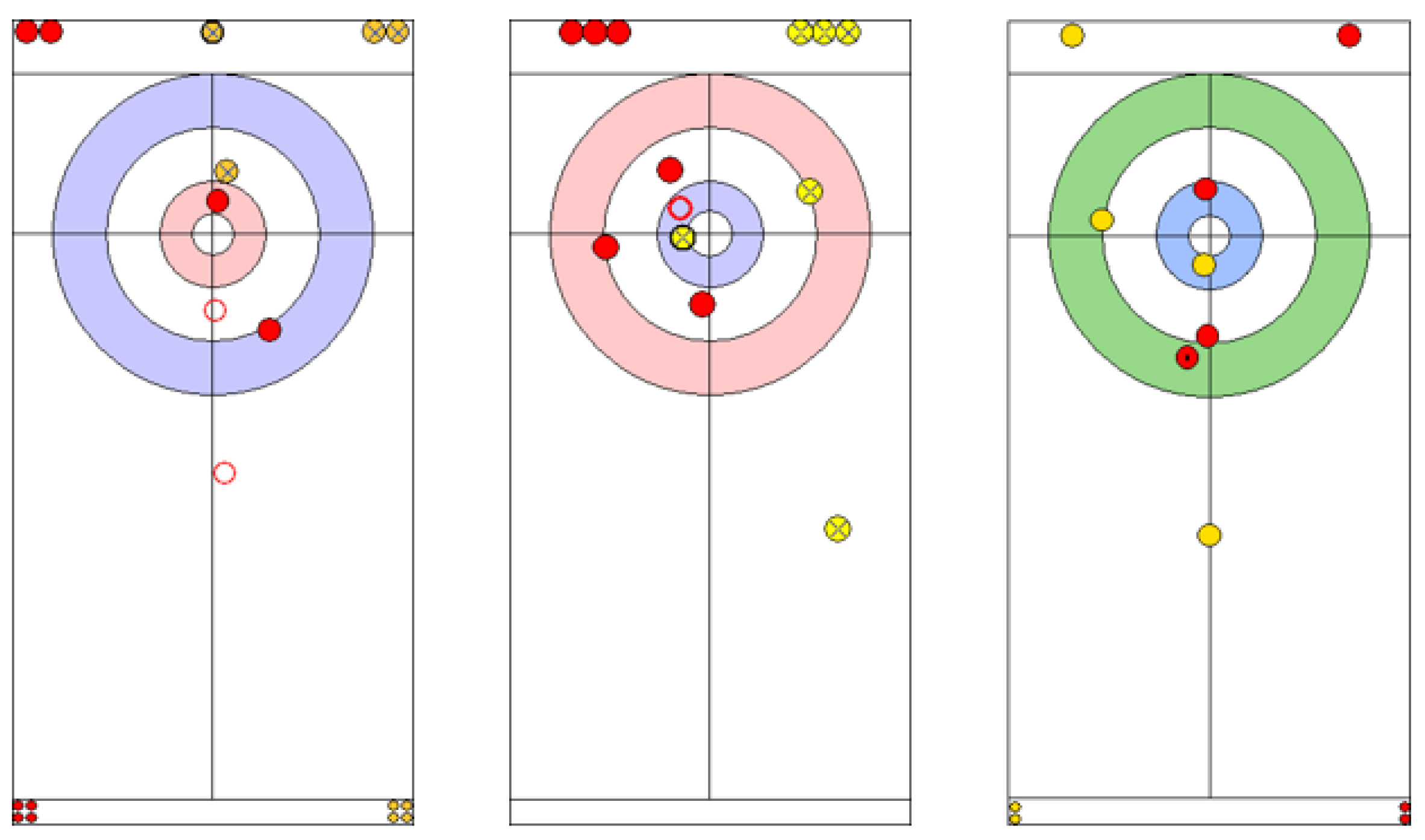
Despite their importance, extracting stone positions from the Results Book is challenging due to inconsistencies in the visual specifications across different editions. Previous studies [6,7,8] proposed that stone position data were extracted by cropping these diagrams—hereinafter referred to as sheet images—from the PDF and detecting stone contours using color-based segmentation. Although this method enables automated extraction for a specific Results Book, it must be adapted to the visual specifications of each document. As shown in Figure 2 and Figure 3, the colors and drawing styles of the sheet images often differ among tournaments. Consequently, substantial manual effort is required to rewrite or adjust the extraction code for each new dataset, which has become a major bottleneck in acquiring large-scale training data for curling AI and in performing tactical analysis that would be revealed by using vast amounts of data, such as the relationship between scoring and shot selection, or the shot selection tendencies of each team.

Ritchie et al. [9] proposed a method for extracting stone coordinates using a circle detection algorithm. However, their pipeline has not been verified for detection accuracy. In addition, it was developed using a dataset containing only 11 tournaments, so there are still concerns about its scalability to a wider range of tournament data. Applying it to a variety of tournament data may require code modifications, such as parameter adjustments.

In recent years, deep learning-based object detection models have been actively and successfully applied to sports image analysis, such as player and ball tracking in various team sports [10,11]. This trend demonstrates the timeliness and effectiveness of adopting a machine learning-based pipeline for this domain.

Inspired by these advancements and to address this limitation, this study proposes a universal stone-coordinate detection model based on object detection techniques, designed to operate independently of individual Results Book specifications.

Compiling a comprehensive database of actual curling match information will not only enable various tactical analyses, but is also expected to contribute to the development of curling AI and its integration with actual curling competition.

Yamamoto et al. [12] utilized Digital Curling [13], a simulation platform designed to reproduce curling games in a computational environment, to develop an expected score distribution prediction model based on neural networks. The expected score distribution represents the probability distribution of scores obtained at the conclusion of an end. Because curling is a sport in which stones cannot always be placed exactly as intended—that is, a sport characterized by inherent uncertainty—scores during an ongoing end are naturally expressed as a distribution.

The original model takes, for each stone, its position (the x- and y-coordinates) and ownership as inputs; Iwasaki et al. [7,8] demonstrated that prediction accuracy is significantly improved by incorporating end state into the model and by training it using actual data provided in the Results Book. The expected score distribution model has since become an essential tool [14] for evaluating ongoing game states in curling, and AI-based players that rely on this model have won several Digital Curling tournaments. This study enables fully automated training data collection, leading to further improvements in prediction performance.

1.1. Contribution

The primary contributions of this study are summarized as follows:

• Proposal for general-purpose stone coordinate extraction from sheet images using object detection model;
• Improving accuracy through semi-supervised learning using pseudo-labels;
• Proposal for a fine-tuning method for new tournament data based on pseudo-labels;
• Quantitative verification of extracted data using a positional error metric;
• Generation of a stone-position dataset with a total of 205,364 positions in 31 tournaments.

1.2. Paper Organization

The rest of this paper is organized as follows. Section 2 provides description of model training and inference settings, performance evaluation methods, methods of application to new tournament data, and positional error verification methods. Section 3 provides training results, effectiveness of an accuracy improvement method, adaptation to new tournament data, and verification of detection error. Section 4 provides a summary of this study, current data acquisition status, and future perspectives.

2. Materials and Methods

This section describes the dataset preparation, the model training settings, and the evaluation methodologies used in this study.

2.1. Preparation

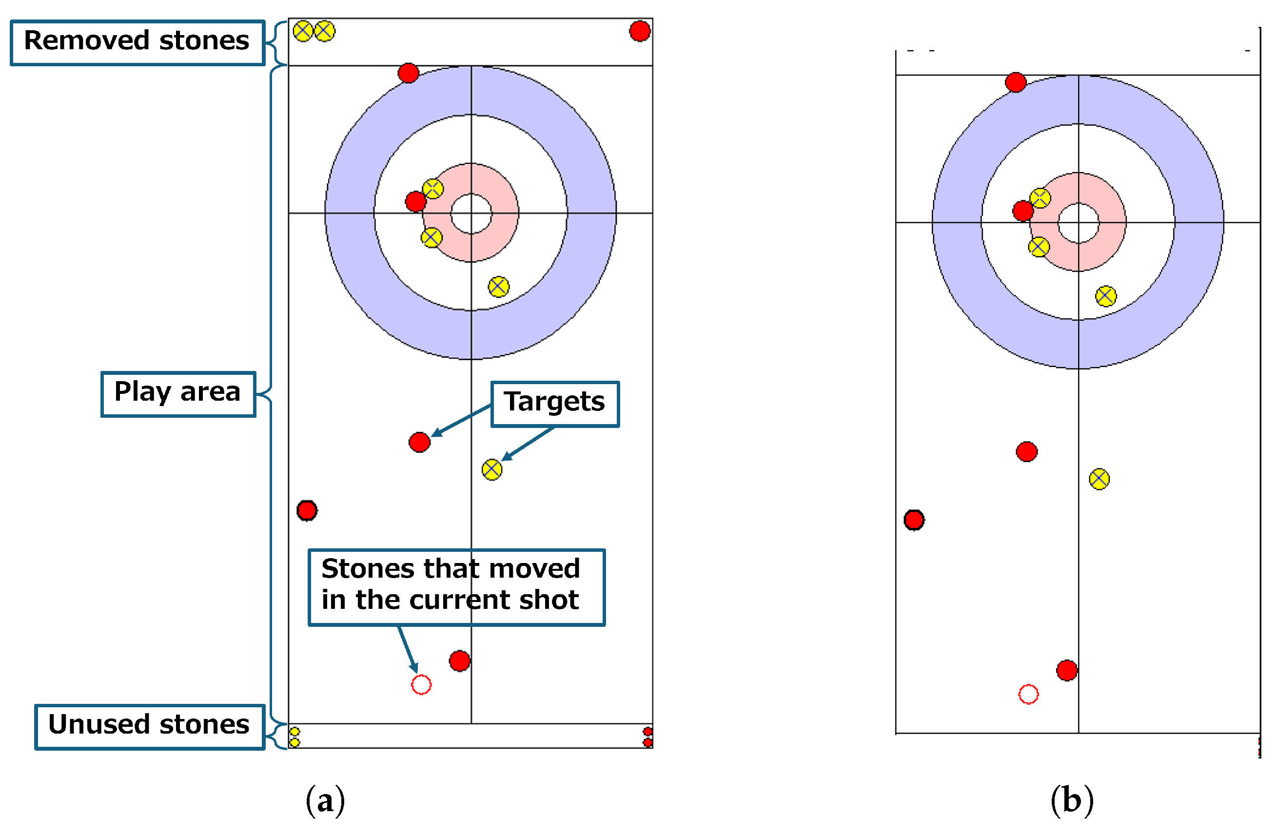
Sheet images were extracted from the Results Book using PyMuPDF (version 1.27.1) [15], a robust Python-based PDF parsing tool. In this study, a total of 20 tournaments and 108,114 images were extracted.

Table 1. Number of images per tournament.

Tournament	Number of Images
ECC 1 2023 Men	6496
ECC 2023 Women	7256
PCCC 2 2022 Men	4167
PCCC 2022 Women	5316
PCCC 2023 Men	3847
PCCC 2023 Women	3364
WJCC 3 2022 Men	1418
WJCC 2022 Women	1594
WJCC 2023 Men	2077
WJCC 2023 Women	2254
WWCC 4 2022	10,807
WMDCC 5 2016	2095
WMDCC 2017	12,970
WMDCC 2018	2325
WMDCC 2019	1346
WMDCC 2021	8296
WMDCC 2022	7860
WMDCC 2023	8182
WMDCC 2024	8213
WMDCC 2025	8231
Total	108,114

¹ European Curling Championship A-division; ² Pan Continental Curling Championship A-division; ³ World Junior Curling Championship A-division; ⁴ World Women’s Curling Championship; ⁵ World Mixed Doubles Curling Championship.

shows the number of images for each tournament. The sheet image depicts the stones present on the sheet, the stones that moved in the current shot, the unused stones, and the stones removed from the play area (Figure 4a). The detection targets are the stones on the sheet. The unused stones and the stones removed from the play area are drawn within the top and bottom 20 pixels of all images. Since these can induce false positives, we masked the top and bottom 20 pixels with white as a preprocessing step. This specific value of 20 pixels was systematically determined as the optimal width that completely hides the removed and unused stones without occluding any valid stones located at the very edge of the play area. As a result, the image input to the model is as shown in Figure 4b.

The proposed model is based on YOLO11n [16] model. This is a lightweight model of the YOLO11 series, one of the more recent versions of YOLO [17], which is widely used in the field of object detection. The distributed model is pre-trained on the COCO dataset [18]. The adoption of YOLO11n is driven by its ability to fulfill the specific requirements of automated stone position extraction through the following rationales:

First, a machine learning-based approach is fundamental to achieving automated adaptability across diverse tournament datasets. While traditional image processing requires manual parameter tuning for each venue, the YOLO-based system can generalize features across graphical formats found in different Results Books, enabling a highly versatile detection pipeline.

Second, the selection of YOLO ensures future scalability in real-time processing. While this study primarily focuses on sheet images in the Results Book, the final goal is to quickly detect stone positions from recorded video in actual curling matches. In this case, YOLO is an effective method in terms of inference speed and accuracy. There are examples of tracking stone trajectories from video of curling matches, and YOLO was used in these cases [19,20]. Therefore, it is believed that using YOLO in camera-based environments is effective. Moreover, we selected the lightweight YOLO11n variant to ensure low-latency inference and high frame-rate processing, prioritizing speed and real-time scalability. Since YOLO11n already achieves an exceptionally high estimated accuracy of 99.37% for the sheet images (as will be detailed in Section 3.2), using larger models (e.g., YOLO11s/m) would require more computational resources without significantly improving the already saturated accuracy.

In this study, the system performance is evaluated by separating it into two primary factors: detection success, that is, whether the stones can be found, and positional accuracy, that is, how precise the detected coordinates are. To achieve this multi-faceted evaluation, we use different definitions of “correct” depending on the specific objective of each research process. For object-level evaluation, a detection is defined as correct if the intersection over union (IoU) between the predicted bounding box and the ground truth box is 0.5 or greater. This definition is based on standard benchmarks in object detection. On the other hand, from the practical perspective of accurately digitizing game situations into a database, an image-level evaluation is conducted. In this case, an image is considered “correct” only if all stones are extracted perfectly without any omissions or false positives; even a single error results in the entire image being marked as incorrect. This strict criterion is essential to ensure the integrity of the database, as a single misplacement in curling can significantly alter the strategic analysis of a given game state. This standard is mainly used in Section 2.3.2.

2.2. Training and Inference Settings

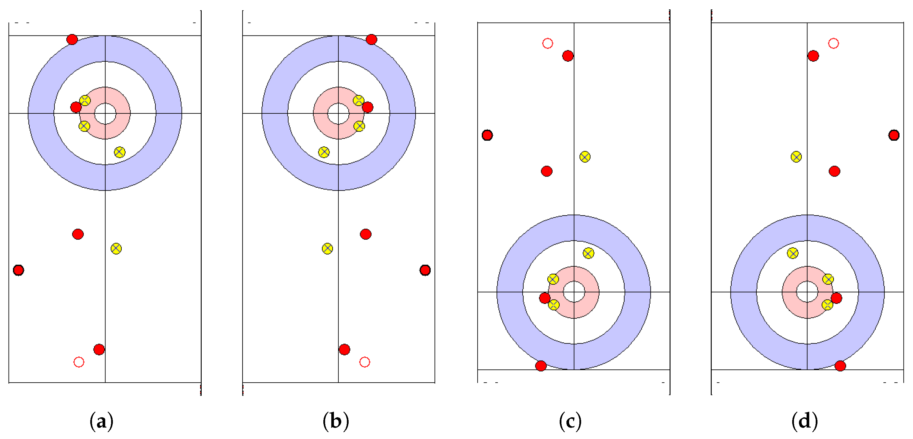
We randomly extracted 50 images from the entire image dataset and annotated them. Since the stone colors in the entire dataset were broadly categorized into two types, red and yellow, two classes were defined: red stones and yellow stones. We randomly split the annotated images into training and validation sets in a ratio of 8:2. Specifically, 40 images were allocated for training, and 10 images were strictly reserved for validation. Since stone detection is independent of the top, bottom, left, and right orientations of the sheet image, the training data were augmented by adding horizontally flipped, vertically flipped, and horizontally–vertically flipped data. Figure 5 illustrates an original image alongside its horizontal, vertical, and combined horizontal–vertical inversions. These flips were applied directly to the pixel coordinate system of the entire image. The coordinate origin strictly remains fixed at the top-left corner (0, 0) across all augmented and original images. Naturally, when stones change positions due to the flipping, the bounding box coordinates in the corresponding label data are mathematically adjusted to match the new positions. This process resulted in 160 training images. The model trained solely on these 160 images is referred to as the pre-trained model in this study. The hyperparameter settings during training are shown in

Table 2. Hyperparameters during YOLO11n training.

Parameter	Value
Batch size	16
Optimizer	AdamW
Learning rate	0.001667
Momentum	0.9
Image size	$300\times 600$
Number of epochs	200

, and the hyperparameter settings during inference are shown in

Table 3. Hyperparameters during YOLO11n inference.

Parameter	Value
IoU threshold 1	0.3
Confidence score threshold for detection 2	0.5

¹ The threshold for eliminating overlaps using non-maximum suppression (NMS). ² A number that indicates how confident the model is in its detection.

. Non-maximum suppression (NMS) [17,21] is applied as a post-processing technique to eliminate redundant overlapping bounding boxes predicting the same stone. In this study, if multiple bounding boxes for the same class (red or yellow) overlap with an intersection over union (IoU) greater than the 0.3 threshold, only the detection with the highest confidence score is retained. Note that the value of 0.5 in Table 3 represents the minimum confidence threshold used to filter out low-certainty detections prior to NMS, distinguishing it from the IoU threshold.

In order to improve accuracy, we carried out semi-supervised learning with labels [22]. It has been reported that there are many research examples using semi-supervised learning approaches in the field of object detection [23]. In particular, in the field of sports, there is an example of improving the accuracy of object detection models using semi-supervised learning for tennis [24].

We randomly extracted 400 images from the entire dataset, ensuring no overlap with the training and validation sets. We performed predictions on these images using the pre-trained model to generate pseudo-labels.

To systematically determine the optimal confidence threshold (which is based on the standard confidence score produced by the YOLO detector, reflecting both objectness and class probability) for this pseudo-labeling process, we conducted a sensitivity analysis using a test set of 500 annotated images that had not been used for training. We evaluated both the pseudo-label quality (Precision) and usable data quantity (Pass Rate) across confidence thresholds of 0.70, 0.75, and 0.80. As shown in the

Table 4. Sensitivity analysis of confidence thresholds for pseudo-labeling. The analysis was conducted on 500 test images using the pre-trained base model. Precision indicates the accuracy of the pseudo-labels, while Pass Rate represents the percentage of images usable for retraining.

Confidence Threshold	Precision	Pass Rate
0.70	1.00000	98.4%
0.75	1.00000	92.0%
0.80	1.00000	49.6%

, the model achieved a perfect Precision of 1.0000 (zero false positives) at all tested thresholds. This guarantees that no erroneous labels were introduced into the pseudo-labeled dataset, entirely mitigating the risk of the model relearning its own errors.

Since label quality was consistently perfect, the selection criterion focuses on maximizing the usable image count for semi-supervised learning. The analysis revealed that while the Pass Rate, that is, the proportion of images where all detected stones exceeded the threshold, remained sufficiently high at 0.70 (98.4%) and 0.75 (92.0%), it dropped sharply to 49.6% at 0.80. Thus, the 0.75 threshold was systematically selected as the optimal balance point. It successfully retains 92.0% of the pseudo-labeled data while providing a conservative safety margin against visually extreme edge cases that might exist in the broader, unlabeled dataset. Raising the threshold to 0.80 would undesirably discard approximately half of the available training images. Consequently, 377 images met this criterion and were added to the original 160 training images. Finally, training was executed using a total of 537 images. During this retraining phase, the same 10 validation images from the initial split were used, and the hyperparameter settings shown in Table 2 were applied.

2.3. Methods of Performance Evaluation

In this experiment, accuracy is evaluated by two methods: evaluating the accuracy using test data obtained by random sampling, and estimating the accuracy of the entire dataset using active testing [25].

2.3.1. Evaluation by Random Sampling

To evaluate the approximate accuracy of the model, we performed an accuracy evaluation by random sampling. As test data, we utilized the same set of 500 manually annotated images that was introduced in Section 2.2 for the threshold sensitivity analysis. The results presented are the learning outcomes obtained from a total of 10 models that were trained using the same training data but with varying random seeds. The final detection relied solely on the single best-performing model. These 10 models were generated for three specific purposes: to ensure statistical reliability by averaging the evaluation metrics, to select the best model for the pipeline, and to have them serve as surrogate models for calculating detection uncertainty in the active testing framework (Section 2.3.2). Varying the random seeds introduces differences in the initial weight distributions and the batch sampling orders during training. These differences cause the models to converge to slightly different local optima, which produces sufficient and intended variability among their predictions to effectively calculate the standard deviation of confidence scores.

As evaluation metrics, we report the mean Precision, Recall, and F1 Score across the 10 models. Furthermore, we present the confusion matrix for the model that achieved the highest F1 Score to examine its performance in detail.

2.3.2. Active Testing

The data from the 500 random samples mentioned above is only about 0.5% of the entire dataset, which makes it difficult to appropriately evaluate the overall accuracy. Therefore, this study applies the active testing method to the object detection task to estimate the overall accuracy with a small amount of test data. This method actively selects high-uncertainty data that the model is likely to err on, performs annotation, and then applies statistical correction based on the results, thereby estimating the accuracy of the entire test dataset with low variance and without bias using a small number of labels. In this experiment, the target images are the 107,164 images remaining after excluding the 40 training images, 10 validation images, 400 retraining images, and 500 randomly sampled test images used so far, totaling 950 images. Let N = 107,164. In this framework, the overall accuracy is derived as $1-R$, where R represents the expected risk of the evaluation model f. The value of R is expressed as follows:

$$R={\displaystyle \frac{1}{N}}\sum _{n=1}^N\mathcal{L}(f\left(x_{i_n}\right),y_{i_n}),$$

(1)

where, $\mathcal{L}$ represents the loss function. In order to calculate this R, it is necessary to calculate the loss for all N instances, which is practically impossible considering the annotation cost. Therefore, the estimator ${\widehat{R}}_{\mathrm{LURE}}$ [25,26] is defined as in Equation (2).

$${\widehat{R}}_{\mathrm{LURE}}={\displaystyle \frac{1}{M}}\sum _{m=1}^M{v}_m\mathcal{L}\left(f\left(x_{i_m}\right),y_{i_m}\right),$$

(2)

where, M is an arbitrary natural number such that $M<N$, and the weight $v_m$ is expressed as in Equation (3).

$$v_m=1+{\displaystyle \frac{N-M}{N-m}}\left({\displaystyle \frac{1}{(N-m+1)q\left(i_m\right)}}-1\right).$$

(3)

In Equation (3), $q\left(i_m\right)$ is the probability of selecting image $x_{i_m}$. This probability is defined to be proportional to the loss between the model’s output and the correct label in terms of treating images that the model is likely to err on as test data. However, since the correct labels are not actually annotated to the images, it is impossible to calculate the loss for each image. Therefore, as an approximation method, the predictions of multiple surrogate models are used. This is because images with a large variance in predictions when inference is performed by multiple surrogate models are considered to have a tendency toward larger actual losses. If this variance is defined as the uncertainty score $\mathcal{U}$, then $q\left(i_m\right)$ is calculated as in Equation (4).

$$q\left(i_m\right)={\displaystyle \frac{U\left(x_{i_m}\right)}{{\sum }_{x\in {\mathcal{D}}_{\mathrm{pool}}^{\left(m\right)}}U\left(x\right)}},$$

(4)

where ${\mathcal{D}}_{\mathrm{pool}}^{\left(m\right)}$ denotes the set of all remaining unlabeled images at step m. In this experiment, a total of 10 models were prepared, which were trained using the same training data as for the construction of the f but with different seeds. For each image, inference was performed with the 10 models, and the standard deviation of their respective confidence scores was calculated. Let $J=10$. Here, no confidence threshold was set during inference. If multiple detected objects exist in one image, the value of the object with the largest standard deviation is used. The above content is expressed as in Equations (5) and (6). However, let $o_x$ be one of the detected objects in image $x_{i_m}$, and let ${\mathrm{conf}}_j$ represent the confidence score calculated by model j.

$$\begin{array}{cc}\hfill \mathcal{U}\left(o_x\right)& =\sqrt{{\displaystyle \frac{1}{J}}\sum _{j=1}^J{(con{f}_j-\overline{conf})}^2},\hfill \end{array}$$

(5)

$$\begin{array}{cc}\hfill \mathcal{U}\left(x_{i_m}\right)& =max\left(\mathcal{U}\left(o_x\right)\right).\hfill \end{array}$$

(6)

We obtained an uncertainty score for each of the N images. Images with a high score mean that there is a large variance in predictions among the models, which allows us to consider them as images containing objects that are more difficult to detect. In this experiment, 500 images were selected as test images by probabilistic sampling without replacement, where the selection probability is proportional to the uncertainty score (Equation (4)). To guarantee non-zero selection probability for all candidates, which is a prerequisite for the unbiasedness of ${\widehat{R}}_{\mathrm{LURE}}$, the probability was bounded from below at $\alpha$ (0.2) times the uniform acquisition probability, following [25]. We annotated the images and performed inference with the model f. That is, $M=500$. $\mathcal{L}(f\left(x_{i_m}\right),y_{i_m})$ is defined as in Equation (7).

$$\mathcal{L}\left(f\left(x_{i_m}\right),y_{i_m}\right)=\left\{\begin{array}{cc}0\hfill & \mathrm{if}f\left(x_{i_m}\right)=y_{i_m},\hfill \\ 1\hfill & \mathrm{if}f\left(x_{i_m}\right)\ne y_{i_m}\hfill \end{array}\right.,$$

(7)

where the condition $f\left(x_{i_m}\right)=y_{i_m}$ denotes that the model f correctly predicts the objects within the image $x_{i_m}$ relative to the ground truth $y_{i_m}$. Specifically, in this study, based on our ground truth definition of an object, a prediction is considered correct if all objects are correctly localized and classified with an IoU $\ge 0.5$. Thus, the loss function evaluates whether the model successfully detects the objects in a single image.

According to the above procedure, we calculated ${\widehat{R}}_{\mathrm{LURE}}$ and obtained the estimated value of the accuracy.

2.4. Methods of Application to New Tournament Data

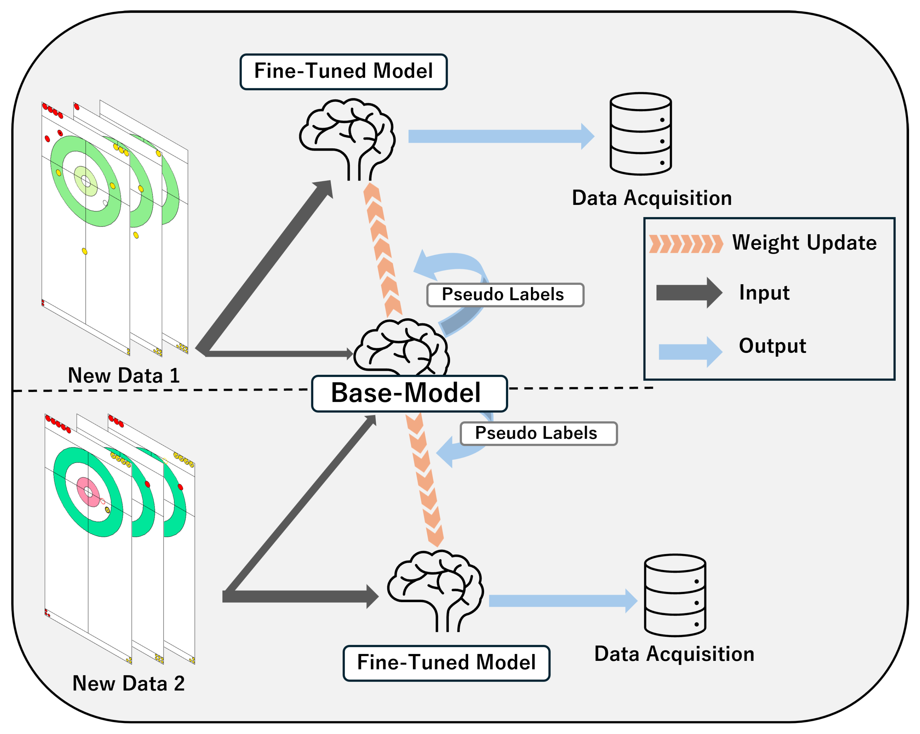
There is a problem where differences in specifications between tournaments could lead to incorrect detection on new tournament data or high costs for program modification. Therefore, this study proposes a method for acquiring stone positions with high accuracy on new tournament data without human cost. In short, the method is self-training with pseudo-labels. To begin with, the model f detected stone positions on new tournament data. We randomly selected 400 images and extracted those in which all detected objects had confidence scores of 0.75 or higher. The selected images were then used to fine-tune the model. The hyperparameter settings during inference followed Table 3. Test images were obtained by annotating 100 images, avoiding overlap with the images used for training. The effectiveness of the proposed method was verified by comparing the model’s prediction results for the test images. Evaluation is performed on data with two different specifications.

2.5. Positional Error Verification

2.5.1. Definition of Positional Error

In this study, there are two possible types of error. One is a detection error that occurs when the model detects stones, and the other is a quantization error that occurs when the stone position is converted into an image.

2.5.2. Quantization Error

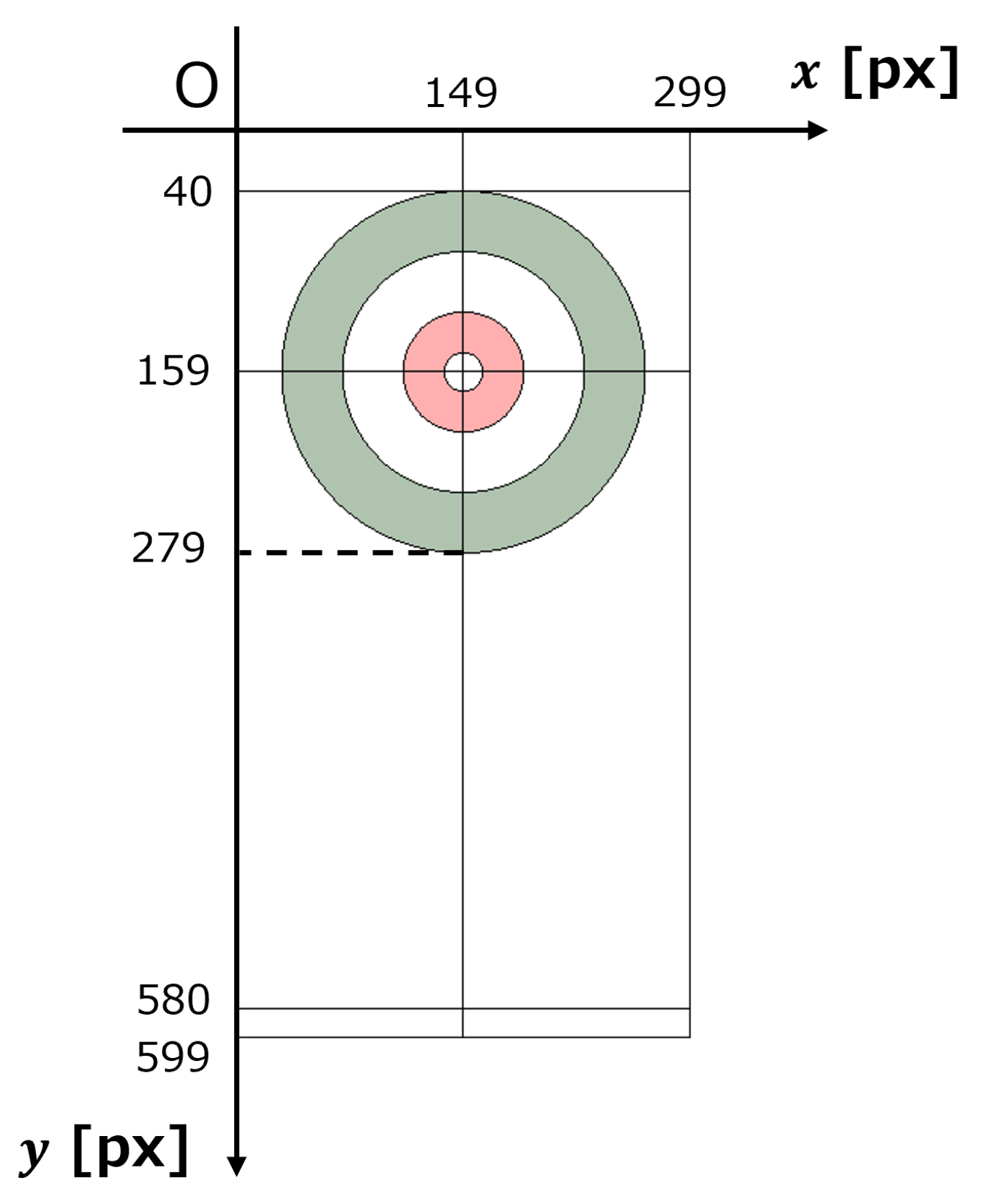
The Shot by Shot image is $300\times 600$ pixels in size and uses the coordinate system shown in Figure 6. In the x-axis direction, the center line (the symmetrical line of the house) should be 149.5 px, but in an actual image, the pixel values must be discretized, so the center line is drawn at 149 px. In other words, it is shifted −0.5 px along the x-axis. In the y-axis direction as well, the top of the house is at 40 px and the bottom is at 279 px, so the tee line should be 159.5 px, but it is drawn at 159 px in an actual image; that is, it is shifted −0.5 px along the y-axis.

2.5.3. Detection Error

The detection error was calculated by measuring the distance between the model’s predicted value and the true value for the center coordinate of the stone. Because the detection model was trained using bounding boxes manually annotated through human visual observation, the original ground truth coordinates inherently contain human-induced positional uncertainty. It is practically impossible for a human annotator to perfectly capture the exact mathematical center of a stone. Consequently, using real images is unsuitable for precisely evaluating microscopic detection errors at the sub-pixel level. To overcome this, we decided to evaluate the true detection error by generating synthetic images where the exact mathematical center coordinates were strictly defined and known without any human error. To ensure these synthetic images were representative of real match conditions, we randomly combined various house colors and stone designs, as well as hollow circles representing pre-collision positions. The method for measuring the detection was as follows.

We generated 1000 images in which stones were randomly positioned within the range of the sheet. For each image, the number of stones was chosen uniformly at random between 1 and 16, and each team (stone color) was constrained to at most 8 stones. Stone positions were sampled so that the x-coordinate followed a distribution peaked at the center line of the sheet, and the y-coordinate a distribution peaked at the tee line. As Figure 2 and Figure 3 show, house color and stone drawing style differ by tournament in the real data, so we prepared the following patterns.

• Six patterns for house color.

  -

  Choose two colors from red, green, and blue and draw each on the inner and outer circles.

• Six patterns for yellow stone.

  -

  Six types (with or without a blue cross mark, as shown in Figure 3).

  -

  Six color types

  (RGB [(255, 255, 0), (255, 220, 0), (255, 200, 50)], which are frequently used in the Results Book).

Since there was little difference in the red stones between tournaments, they were one type of RGB (255, 0, 0). For each image, we generated an appropriate number of red and yellow stones, ranging from 0 to 8 respectively. This resulted in a total of 8020 stones across the 1000 images. In addition, to resemble actual data, we randomly placed hollow circles. These were the positions where the stones were before the shot and were drawn to show that they moved due to collisions between stones. In other words, these were not subject to detection.

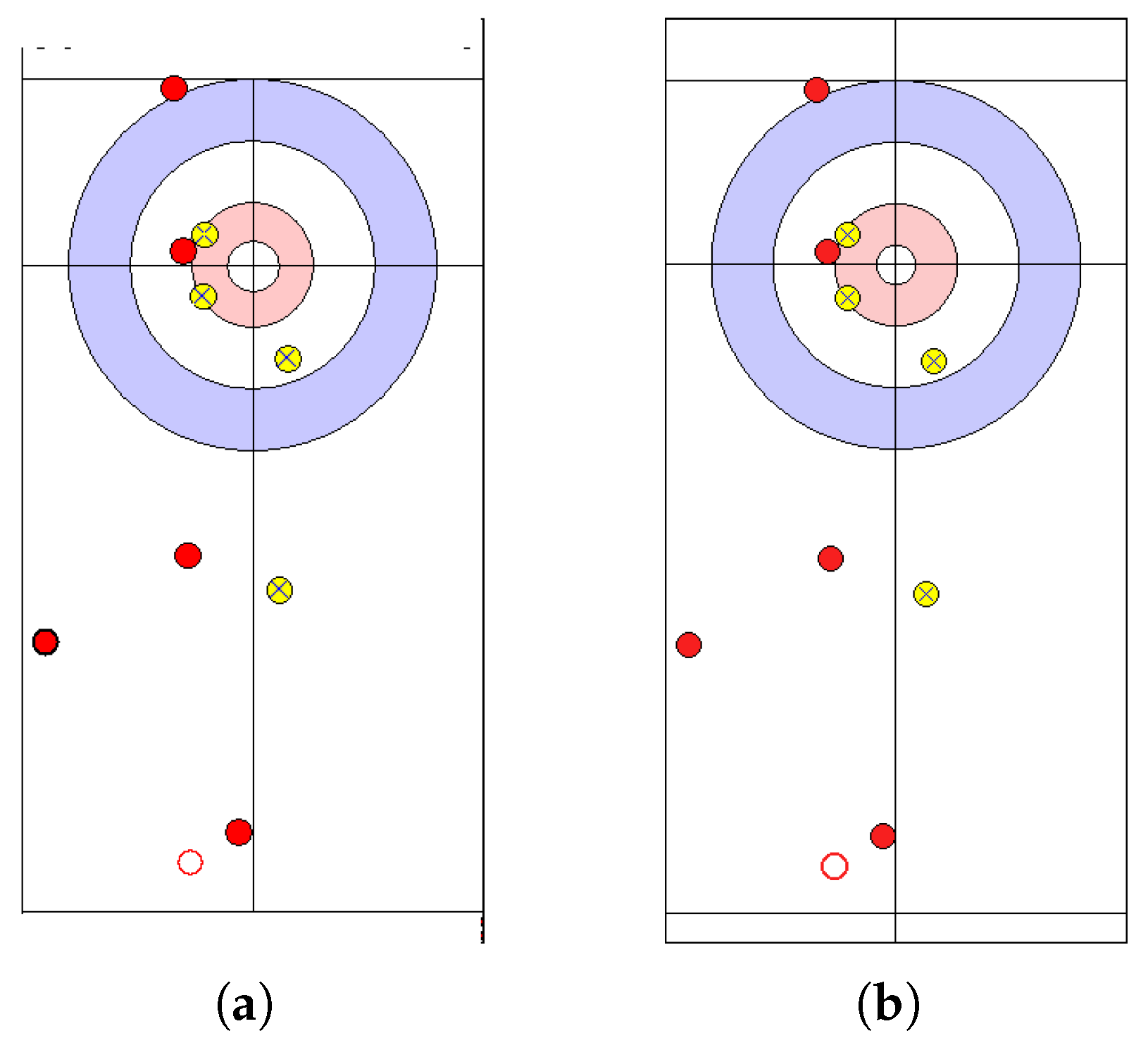
We obtained the label data for the center coordinates of the stones from the generated images and used these as the ground truth. To quantitatively evaluate the visual fidelity of our synthetic images, we created a strictly matched synthetic image that imitated a specific real image by extracting exact color information (RGB values) and matching the stone coordinates. The resulting image pair, now shown in Figure 7, achieved a high structural similarity index measure (SSIM) of 0.855. SSIM is a widely used metric that evaluates image similarity based on three visual features: luminance, contrast, and structure [27]. The high SSIM score quantitatively demonstrates that our generation method accurately mimics visual features of actual images.

And then, we tried to detect the stones and obtained the coordinates. We defined the L2 norm of the ground truth and predicted values as the detection error.

3. Results

This section presents the results of the model’s performance evaluation, overall accuracy estimation, application to new tournament data, and positional error verification.

3.1. Performance Evaluation

In this section, we present the results of the accuracy evaluation performed on the 500 test data instances extracted by random sampling. In this experiment, a total of 10 models were used, trained with the same training data but with varying seeds.

Table 5. Results (mean ± std). The standard deviations across the 10 training seeds are included in the cells to demonstrate model stability.

Method	Class	Precision	Recall	F1 Score
Supervised Learning	Red	$0.99941\pm 0.00058$	$0.99993\pm$ 0.00023	$0.99967\pm 0.00037$
	Yellow	$0.99977\pm 0.00037$	$0.99879\pm 0.00081$	$0.99928\pm 0.00045$
	Overall	$0.99959\pm 0.00041$	$0.99937\pm 0.00043$	$0.99948\pm 0.00033$
Semi-Supervised Learning	Red	$0.99948\pm 0.00070$	$1.00000\pm$ 0.00000	$0.99974\pm 0.00035$
	Yellow	$0.99992\pm 0.00024$	$0.99932\pm 0.00097$	$0.99962\pm 0.00050$
	Overall	$0.99970\pm 0.00034$	$0.99966\pm 0.00048$	$0.99968\pm 0.00036$

shows the Precision, Recall, and F1 Score for the model trained using 160 images including data augmentation. Each value is the average from the 10 models.

3.1.1. Supervised Learning with Annotated Data

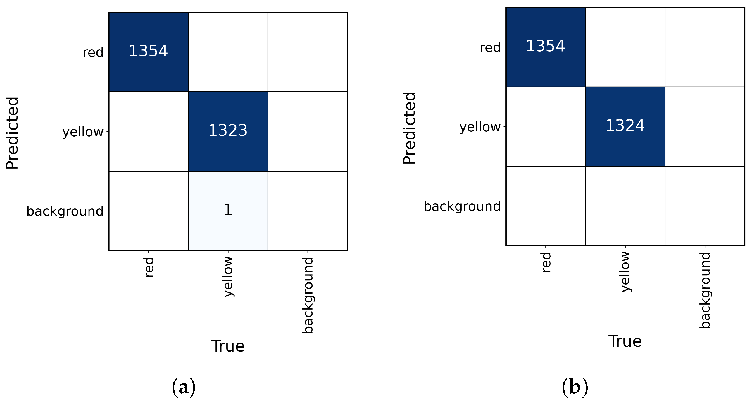
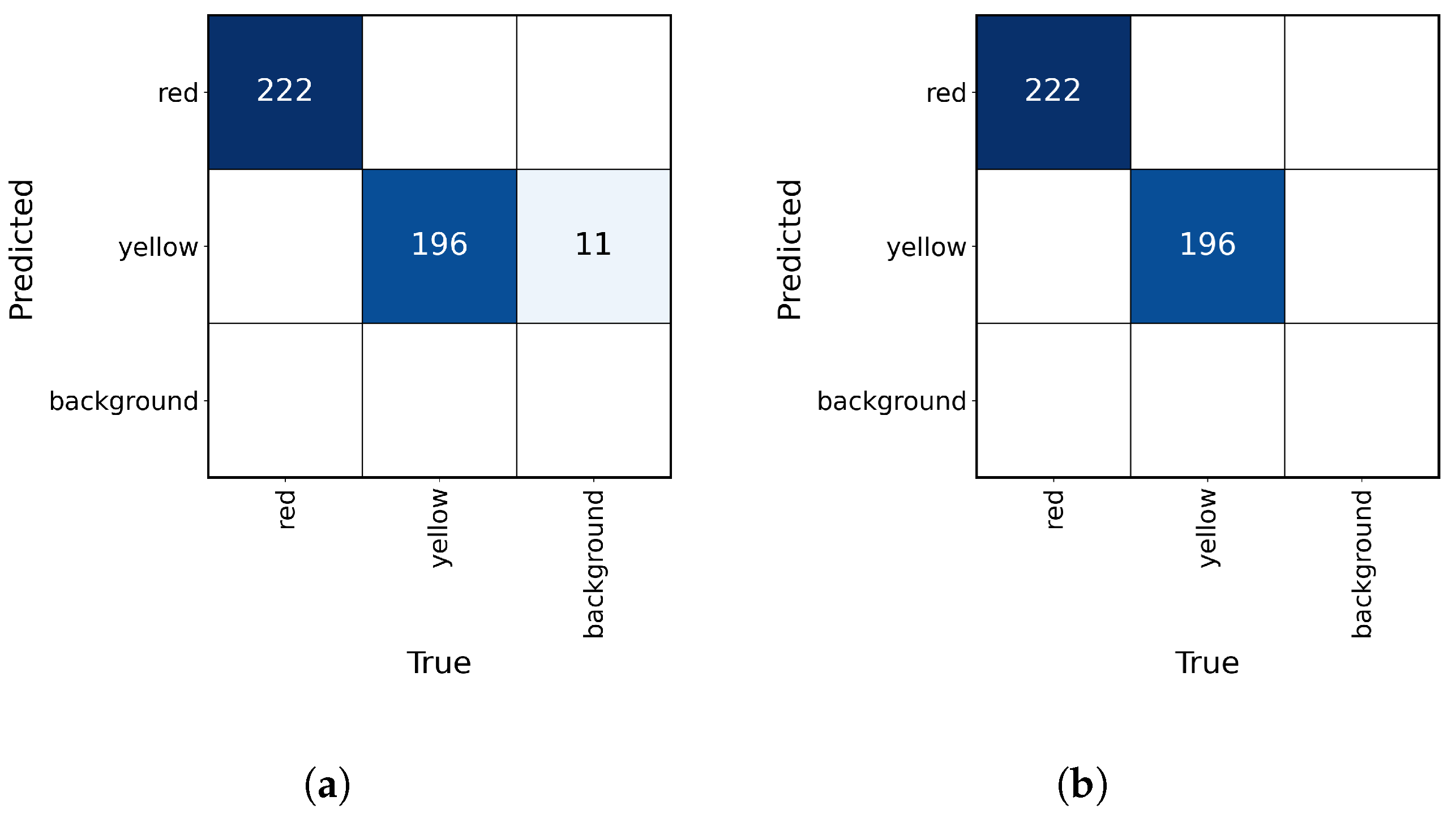
Considering the results by class, although the Precision is higher for yellow, the Recall is higher for red. This implies that the probability of a detected yellow stone actually being yellow is high, and the probability of not missing a red stone when it is actually present is high. This can be interpreted as yellow having a tendency to be detected cautiously to avoid false positives, while red tends to be detected across a wider range to prevent missed detections. Furthermore, the confusion matrix for the detection results of the best model is shown as Figure 8a. This model will be referred to as model $f^{-}$ below. Each cell value represents the number of detected instances for each class, with 1354 red stones and 1323 yellow stones detected. However, it is clear that one instance was missed.

3.1.2. Semi-Supervised Learning with Pseudo-Labels

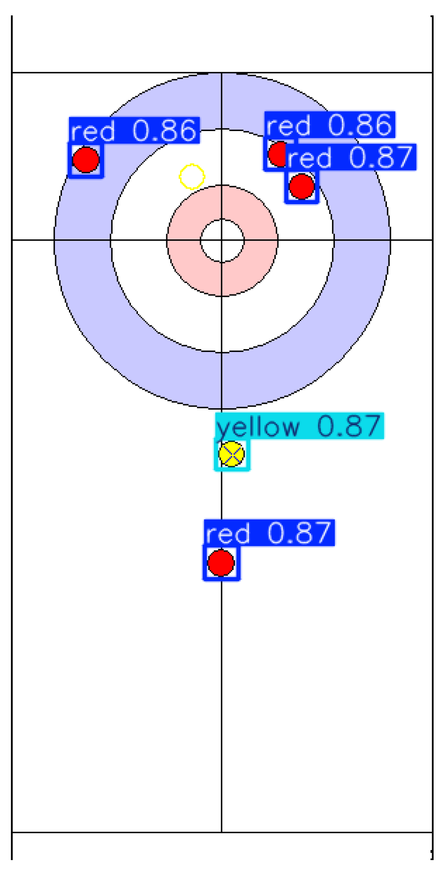
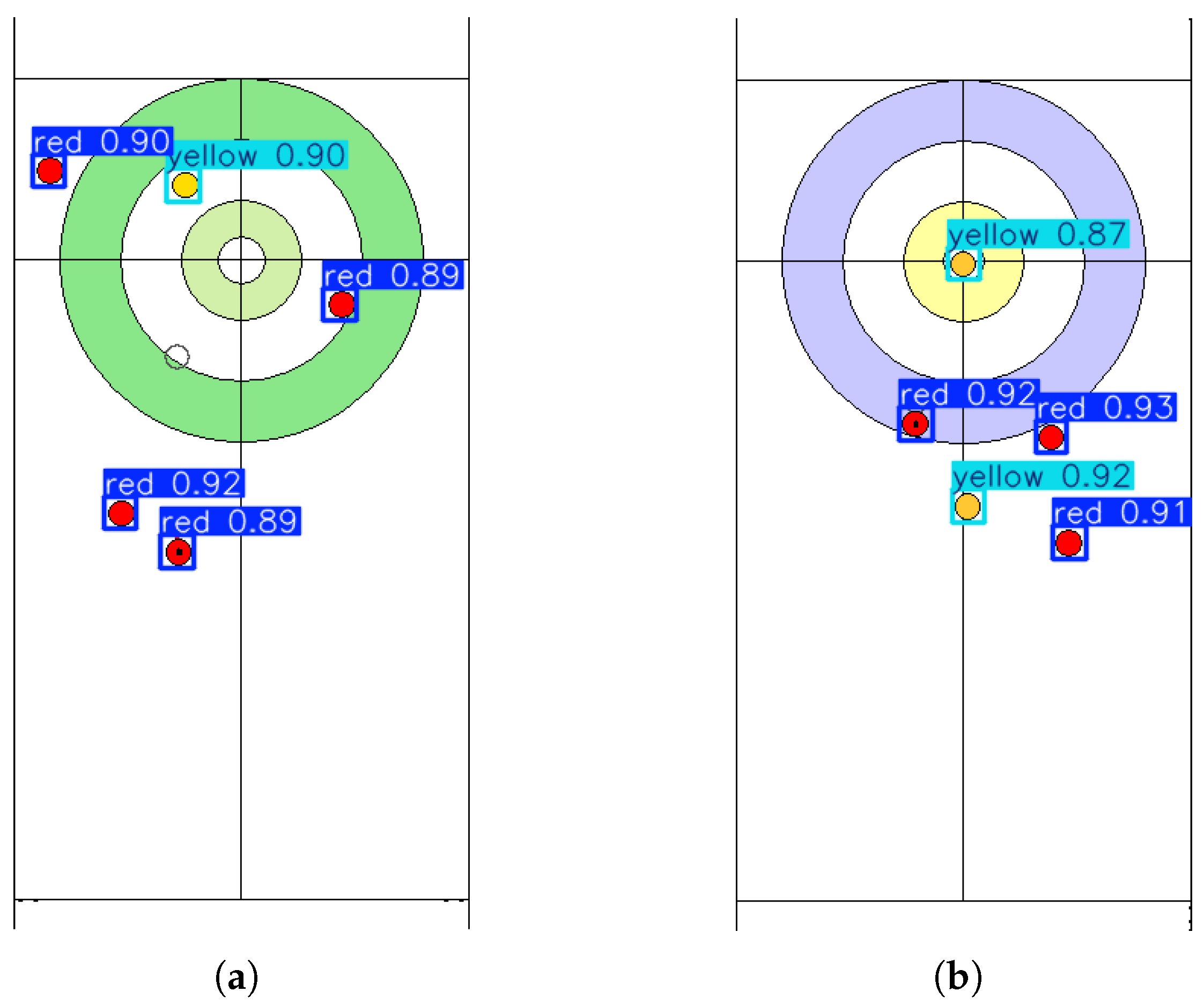
We verified whether accuracy improves by fine-tuning with pseudo-labels. According to the Table 5, each value increased, so it can be said that the accuracy improved. The model obtained by performing semi-supervised learning on model $f^{-}$ is designated as model f. The confusion matrix of the detection results for model f is shown in Figure 8b. It is confirmed that all objects were detected correctly. Figure 9 shows an example of actual stone detection.

3.2. Estimating Accuracy for All Data

Using active testing [25], we estimated the accuracy of model f for all 107,164 data points. From Equation (2), ${\widehat{R}}_{\mathrm{LURE}}=0.0063$, resulting in an estimated accuracy of 99.37%.

3.3. Results for New Tournament Data

3.3.1. New Tournament Data 1

The result of the model f is shown in Figure 10a, and 11 false positives occurred. This indicates that if the model f is used directly on new tournament data, there will be a certain percentage of false detections, and it will not be a highly accurate detection method. The results of the fine-tuned model are shown in Figure 10b. The model correctly detected all objects. Figure 11a shows an example of actual stone detection.

3.3.2. New Tournament Data 2

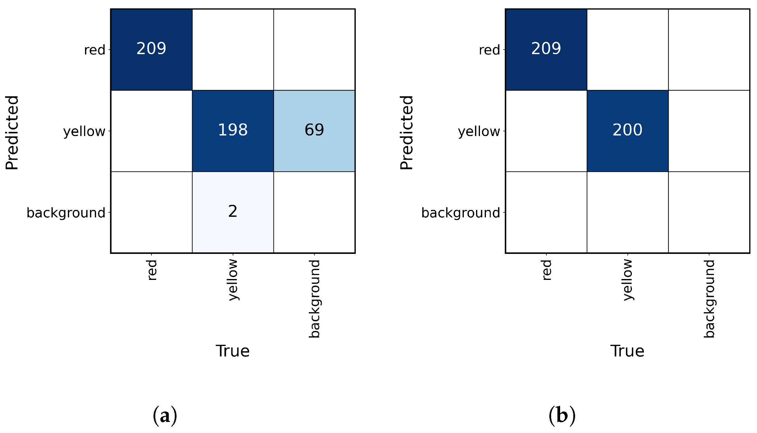
The result of the model f is shown in Figure 12a. Sixty-nine false positives and two false negatives occurred. The result of the fine-tuned model is shown in Figure 12b. As with new tournament data 1, the accuracy tends to improve. Figure 11b shows an example of actual stone detection.

In summary, it turned out that by fine-tuning using pseudo-labels for new tournament data, accuracy could be improved without the effort of modifying the program. When we actually acquire data, we follow the processes shown in Figure 13.

3.4. Detection Error Verification

We measured the 1000 generated images using the model f. When all 8020 objects were correctly detected, the average detection error defined as the Euclidean distance (L2 norm) between the predicted and ground truth center coordinates was 0.472 px, with a standard deviation of 0.228 px. The radius of the stone in the image is about 9 px, so the detection error is about one-twentieth of the radius of the stone.

To clarify the relationship between pixel coordinates and real-world spatial coordinates, we converted this error into physical units. Given that the standard radius of an actual curling stone is approximately 14.5 cm and its radius in the image is about 9 px, 1 pixel corresponds to roughly 1.61 cm. Thus, the average detection error of 0.472 px translates to a real-world positional error of approximately 0.76 cm.

Regarding the detection error evaluated using synthetic images, there are limitations when transferring these results to real-world scenarios. Because synthetic images are mathematically perfect, they lack the microscopic compression artifacts or anti-aliasing noise inherent in actual PDF formats. Therefore, the evaluated error of 0.472 px represents a theoretical lower bound under ideal conditions, and such rendering noises might slightly increase the detection error in practical applications to real images.

As discussed in Section 2.5.2, however, converting physical coordinates into a digital pixel grid inevitably introduces a rounding error of up to 0.5 px from the true center. The fact that the model’s error remains below this threshold demonstrates that the detection is performing at the maximum possible resolution of the image format. Moreover, it is important to note the inherent discrepancies in the source data. The stone positions in the Results Book are recorded manually by official recorder based on visual observation during the match. Consequently, the “ground truth” images themselves already contain a degree of human-induced error relative to the actual positions on the ice.

In actual curling competitions, a sub-centimeter difference can sometimes determine the outcome of a shot. However, when constructing a database from Results Books, we must consider the inherent limitations of the data source. Because, as mentioned above, the model’s detection error (0.472 px) is strictly smaller than the 0.5 px quantization limit and the inevitable human-induced recording errors present in the original PDFs, achieving higher accuracy from this specific medium is fundamentally impossible. For the practical purpose of training curling AI for macroscopic tactical evaluation such as expected score distributions, this sub-centimeter error is overwhelmingly overshadowed by the original recording errors, making it practically sufficient and highly acceptable for our database construction.

4. Conclusions

In this study, we proposed the application of object detection as a method for acquiring stone position data from actual curling matches, and as a result of the validation, we were able to build a model that could detect stone position with 99.37% accuracy. Furthermore, we clarified that we can automatically construct a high-accuracy model for new tournament data by self-training with pseudo-labels. In addition, we found that the positional error was sufficiently smaller than the radius of the stone.

However, this study has several limitations. First, the data acquisition framework heavily relies on the availability and static format of the Results Books, restricting its application in matches where such documents are not published. If there are errors or missing images in the Results Book, we are forced to rely on that data. Second, many of the threshold parameters and the number of re-training data used in this study were determined based on values judged to be appropriate through qualitative evaluation. Therefore, there is a possibility that they may not be optimal parameters. In the future, it will be necessary to verify whether these parameters are appropriate and whether changing them will improve accuracy of the model. Furthermore, since this study confirmed the construction of a model capable of high-precision detection, future research must take identifying images where errors occur and how to address such cases into consideration.

Currently, we are building a database by using this model to acquire stone coordinates and combining them with the various game information from the Results Book. At the time of writing, we have obtained stone coordinates and game information for 205,364 situations from 31 tournaments.

In the future, we plan to build a tool to automate the database creation of the Results Book looking ahead to new ones. As an application of this technology, it can be also possible to detect stone positions from video footage of actual games. Recently, various advanced video object detection methods have been proposed for dynamic environments. These include approaches utilizing temporal contexts and motion priors [28,29], as well as tracking models in other dynamic sports [30]. Applying these state-of-the-art video tracking techniques to our static detection model will be a highly promising future direction for real-time curling video analysis. Since many tournaments do not have a Results Book, this technology is essential from the perspective of obtaining more data on actual games. For this, it will be critical to address specific technical challenges, such as dealing with identifying the target frame resulting from camera switching, viewpoint changes from varying camera angles, and optimizing the model architectures to meet strict real-time processing requirements. We aim to promote the creation of a database that compiles information from various curling games, including video, and utilize it for the training of curling AI and data analysis.

References

1. Zacharias, E.; Robak, N.; Passmore, S. An examination of studies related to the sport of curling: A scoping review. Front. Sport. Act. Living 2024, 6, 1291241. [Google Scholar] [CrossRef] [PubMed]
2. Han, Y.; Zhou, Q.; Duan, F. A game strategy model in the digital curling system based on NFSP. Complex Intell. Syst. 2022, 8, 1857–1863. [Google Scholar] [CrossRef]
3. Lee, K.; Kim, S.A.; Choi, J.; Lee, S.W. Deep reinforcement learning in continuous action spaces: A case study in the game of simulated curling. In Proceedings of the 35th International Conference on Machine Learning; PMLR: Cambridge, MA, USA, 2018; pp. 2937–2946. [Google Scholar]
4. Brunner, M.; Riesen, K. Comparing Learning Methods to Enhance Decision-Making in Simulated Curling. In Joint IAPR International Workshops on Statistical Techniques in Pattern Recognition (SPR) and Structural and Syntactic Pattern Recognition (SSPR); Springer Nature: Cham, Switzerland, 2024; pp. 156–165. [Google Scholar]
5. CURLIT. Curling Results. Available online: https://curlit.com/results (accessed on 11 November 2025).
6. Myslik, J. Curling Analytics. Available online: https://www.jordanmyslik.com/portfolio/curling-analytics/ (accessed on 1 March 2026).
7. Iwasaki, T.; Noguchi, W.; Tamura, Y.; Aihara, S.; Yamamoto, M. Creation of training data and training for prediction model of curling scores using real game data. In Proceedings of the 12th International Conference on Sport Sciences Research and Technology Support (icSPORTS), Porto, Portugal, 21–22 November 2024; pp. 168–179. [Google Scholar]
8. Iwasaki, T. Training Method to Improve the Accuracy of Prediction Model of Curling Scores. Master’s Thesis, Hokkaido University, Sapporo, Japan, 2025. [Google Scholar]
9. Ritchie, R.; Leblanc, A.; Loughin, T. Opening the House: Datasets for Mixed Doubles Curling. arXiv 2025, arXiv:2512.16574. [Google Scholar] [CrossRef]
10. Şah, M.; Direkoğlu, C. Review and evaluation of player detection methods in field sports: Comparing conventional and deep learning based methods. Multimed. Tools Appl. 2023, 82, 13141–13165. [Google Scholar] [CrossRef]
11. Moreira, C.; Ferreira, L.; Coelho, P.J. A comprehensive review of ball detection techniques in sports. PeerJ Comput. Sci. 2025, 11, e3079. [Google Scholar] [CrossRef] [PubMed]
12. Yamamoto, M.; Kato, S.; Iizuka, H. Learning of Expected Scores Distribution for Positions of Digital Curling. In Proceedings of the Workshop on Curling Informatics (WCI 2018), Kitami, Japan, 2–3 August 2018; pp. 8–9. [Google Scholar]
13. Ito, T.; Kitasei, Y. Proposal and Implementation of “Digital Curling”. In Proceedings of the 2015 IEEE Conference on Computational Intelligence and Games, Tainan, Taiwan, 31 August–2 September 2015; pp. 469–473. [Google Scholar]
14. Yamamoto, M. Artificial Intelligence Approaches for Curling; IEICE Technical Report; CQ2022-32; IEICE: Tokyo, Japan, 2022; Volume 122, p. 49. [Google Scholar]
15. Artifex Software, Inc. PyMuPDF, Version 1.26.6. GitHub Repository. 2025. Available online: https://github.com/pymupdf/PyMuPDF (accessed on 5 February 2026).
16. Jocher, G.; Qiu, J. Ultralytics YOLOv11, Version: 11.0.0. GitHub Repository, 2024; License: AGPL-3.0. Available online: https://github.com/ultralytics/ultralytics (accessed on 11 November 2025).
17. Redmon, J.; Divvala, S.; Girshick, R.; Farhadi, A. You Only Look Once: Unified, Real-Time Object Detection. In Proceedings of the IEEE Conference on Computer Vision and Pattern Recognition, IEEE Computer Society, Las Vegas, NV, USA, 27–30 June 2016; pp. 779–788. [Google Scholar]
18. Lin, T.Y.; Maire, M.; Belongie, S.; Hays, J.; Perona, P.; Ramanan, D.; Dollár, P.; Zitnick, C.L. Microsoft COCO: Common Objects in Context. In European Conference on Computer Vision; Springer International Publishing: Cham, Switzerland, 2014; pp. 740–755. [Google Scholar]
19. Aihara, S.; Chen, G.; Hara, R.; Nakagawa, M.; Ogasawara, A.; Yanagi, H.; Takegawa, Y.; Ito, T.; Masui, F. Development of a Simple Tracking System to Monitor Curling Stone Dynamics. In Proceedings of the 12th International Conference on Sport Sciences Research and Technology Support (icSPORTS), Porto, Portugal, 21–22 November 2024; pp. 22–33. [Google Scholar]
20. Guo, Y.; Jin, J.; Zhao, H.; Jiang, Y.; Li, D.; Shen, Y. High-Precision prediction of curling trajectory multivariate time series using the novel CasLSTM approach. Sci. Rep. 2025, 15, 3468. [Google Scholar] [CrossRef] [PubMed]
21. Hosang, J.; Benenson, R.; Schiele, B. Learning non-maximum suppression. In Proceedings of the IEEE Conference on Computer Vision and Pattern Recognition, Honolulu, HI, USA, 21–26 July 2017. [Google Scholar]
22. Lee, D.H. Pseudo-label: The simple and efficient semi-supervised learning method for deep neural networks. In Workshop on Challenges in Representation Learning; ICML: San Diego, CA, USA, 2013; Volume 3, p. 896. [Google Scholar]
23. Shehzadi, T.; Ifza, I.; Liwicki, M.; Stricker, D.; Afzal, M.Z. Semi-supervised object detection: A survey on progress from cnn to transformer. Sensors 2026, 26, 310. [Google Scholar] [CrossRef] [PubMed]
24. Zhao, Y. Progressive Semi-Supervised Learning for Enhanced Detection in Tennis Sport: From Simple to Complex. IEEE Access 2024, 12, 84352–84362. [Google Scholar] [CrossRef]
25. Kossen, J.; Farquhar, S.; Gal, Y.; Rainforth, T. Active testing: Sample-efficient model evaluation. In International Conference on Machine Learning; PMLR: Cambridge, MA, USA, 2021; pp. 5753–5763. [Google Scholar]
26. Farquhar, S.; Gal, Y.; Rainforth, T. On statistical bias in active learning: How and when to fix it. arXiv 2021, arXiv:2101.11665. [Google Scholar] [CrossRef]
27. Wang, Z.; Bovik, A.C.; Sheikh, H.R.; Simoncelli, E.P. Image quality assessment: From error visibility to structural similarity. IEEE Trans. Image Process. 2004, 13, 600–612. [Google Scholar] [CrossRef] [PubMed]
28. Yu, T.; Chen, C.; Zhou, Y.; Hu, X. Improving surveillance object detection with adaptive omni-attention over both inter-frame and intra-frame context. In Proceedings of the Asian Conference on Computer Vision, Macao, China, 4–8 December 2022; pp. 2697–2712. [Google Scholar]
29. Wang, X.; Hu, X.; Chen, C.; Fan, Z.; Peng, S. Illuminating vehicles with motion priors for surveillance vehicle detection. In Proceedings of the 2020 IEEE International Conference on Image Processing (ICIP), Abu Dhabi, United Arab Emirates, 25–28 October 2020; pp. 2021–2025. [Google Scholar]
30. Vicente-Martínez, J.A.; Márquez-Olivera, M.; García-Aliaga, A.; Hernández-Herrera, V. Adaptation of YOLOv7 and YOLOv7_tiny for soccer-ball multi-detection with DeepSORT for tracking by semi-supervised system. Sensors 2023, 23, 8693. [Google Scholar]
Figure 1. An example of a Shot by Shot page in a Results Book. This page illustrates the game progression of an end—in which the red team plays first, the two teams alternate shots, and the yellow team ultimately scores two points—with the images of the stone positions arranged in the order of the shots.
Applsci 16 03453 g001
Figure 2. Differences in sheet images depending on the tournament. The house colors and stone designs vary from tournament to tournament.
Applsci 16 03453 g002
Figure 3. Differences in yellow stones depending on the tournament. The colors differ slightly, and the designs also vary among the Results Books.
Applsci 16 03453 g003
Figure 4. An example of a sheet image: (a) Sheet image description. Only stones in the play area are targets. (b) Input image. The top and bottom 20 pixels are masked with white to prevent false positives.
Applsci 16 03453 g004
Figure 5. Examples of data augmentation using image inversion: (a) Original image. (b) Horizontally flipped image. (c) Vertically flipped image. (d) Horizontally and vertically flipped image. The coordinate origin (0, 0) remains fixed at the top-left corner across all images.
Applsci 16 03453 g005
Figure 6. The coordinate system of an image. The image size is 300 × 600 and the upper left corner is the origin. The tee line is drawn at y = 159 , and the center line is drawn at x = 149 .
Applsci 16 03453 g006
Figure 7. Visual comparison between an actual image and a generated image: (a) Actual image. (b) Generated image. The structural similarity index measure (SSIM) between them is 0.855, demonstrating high visual fidelity.
Applsci 16 03453 g007
Figure 8. Confusion matrix. Each value represents the total number of detected objects: (a) Inference results for the model trained with annotated data. There is 1 object that is actually a yellow stone but is detected as background, i.e., 1 false negative. (b) Inference results for the model fine-tuned with pseudo-labels. All objects are detected correctly.
Applsci 16 03453 g008
Figure 9. Stone detection example. The numbers represent the confidence scores. All stones detected with high confidence score.
Applsci 16 03453 g009
Figure 10. Confusion matrix for new tournament data 1. Each value represents the total number of detected objects: (a) Inference results for the model f on new tournament data. There are 11 objects that is actually background but is detected as a yellow stone, i.e., 11 false positives. (b) Inference results for the model fine-tuned with pseudo-labels on new tournament data. All objects are detected correctly.
Applsci 16 03453 g010
Figure 11. Stone detection example on new tournament data. All stones detected with high confidence score: (a) Prediction results of sheet images for “World Men’s Curling Championship 2025” (WMCC2025). (b) Prediction results of sheet images for “World Women’s Curling Championship 2025” (WWCC2025).
Applsci 16 03453 g011
Figure 12. Confusion matrix for new tournament data 2. Each value represents the total number of detected objects: (a) Inference results for the model f on new tournament data. There are 69 objects that is actually background but is detected as a yellow stone, i.e., 69 false positives. There are 2 objects that are actually yellow stones but are detected as background, i.e., 2 false negatives. (b) Inference results for the model fine-tuned with pseudo-labels on new tournament data. All objects are detected correctly.
Applsci 16 03453 g012
Figure 13. Flow diagram for acquiring new tournament data. We acquire new tournament data using a model fine-tuned with pseudo-labels on them.
Applsci 16 03453 g013