Article

Design of Optimized Time-Shifted Sine Motion Profiles for High-Speed, Low-Vibration Motion

by
Chang-Wan Ha
1 and
Dongwook Lee
2,*
1
Department of Mechanical Engineering, Kookmin University, 77, Jeongneung-ro, Seongbuk-gu, Seoul 02707, Republic of Korea
2
Department of Mechanical & Automotive Engineering, Kongju National University, 1223-24, Cheonan-daero, Seobuk-gu, Cheonan-si 31080, Republic of Korea
*
Author to whom correspondence should be addressed.
Appl. Sci. 2026, 16(6), 3098; https://doi.org/10.3390/app16063098
Submission received: 18 February 2026 / Revised: 18 March 2026 / Accepted: 19 March 2026 / Published: 23 March 2026
(This article belongs to the Special Issue Advanced Control Systems and Control Engineering)

Abstract

High-speed precision positioning systems require motion profiles that achieve rapid transfer while suppressing motion-induced vibration. Conventional time-optimal trajectories often minimize travel time at the expense of residual vibration, which prolongs settling and degrades positioning accuracy. This paper proposes a systematic framework for designing optimized time-shifted sine motion profiles that explicitly incorporate vibration suppression in the frequency domain. By integrating time-domain profile construction with Laplace-domain analysis, motion profiles are derived in a unified manner from 1st-order to generalized n th -order forms. A key theoretical result shows that the residual vibration amplitude after motion completion is proportional to the magnitude of | s X ( s ) | evaluated at the system poles, providing a clear analytical basis for a closed-form zero placement strategy. Explicit algebraic design conditions are obtained without iterative numerical optimization. Simulation-based case studies demonstrate that the proposed approach drastically reduces transient and residual vibrations while maintaining competitive motion completion times compared with time-optimal designs. Robustness is quantitatively evaluated using insensitivity and high-frequency roll-off metrics, revealing that increasing the profile order improves uncertainty tolerance by approximately 20 dB/decade per order. Furthermore, a short-stroke scenario shows that lower-order sine profiles can be advantageous under moderate uncertainty. The proposed framework provides a practical guideline for vibration-aware high-speed motion control.

1. Introduction

In high-speed precision positioning systems, the motion profile is recognized as a core element that goes beyond simply generating smooth trajectories in the time domain; it involves designing the frequency characteristics of the input signal to minimize vibrations caused by the movement of mechanical components [1,2]. The trapezoidal velocity profile, widely adopted in industrial applications, offers the advantage of rapid target positioning by maximizing actuator performance. However, it includes high-frequency components at points where acceleration changes discontinuously, acting as a cause for inducing residual vibrations in the system [3,4,5]. Such vibrations not only decrease the productivity of the entire process by increasing the settling time but can also lead to wear on mechanical parts or damage to the workpiece. To compensate for this, the S-curve profile was proposed to make acceleration changes gradual by limiting the jerk—the derivative of acceleration—to a finite value [6]. However, the S-curve inherently poses a risk of inducing motion-induced vibration due to abrupt jerk changes at segment switching instants [7].
The fundamental cause of structural vibration induced by motion profiles is that the frequency components of the reference command overlap with the system’s vibration modes, thereby inducing motion-induced vibration [1,3]. In particular, polynomial-based motion profiles are often defined piecewise to satisfy boundary conditions [8], and the rapid changes occurring at segment switching instants act as a factor that increases high-frequency components. To address these limitations, recent research has focused on trigonometric motion profiles, which provide smoother transitions between segments and reduce the likelihood of exciting motion-induced vibration [9]. This research trend is also closely linked to recent industrial demands. For example, high-precision stages used in photolithography are undergoing continuous weight reduction and speed enhancement for higher throughput [10]. Similarly, robot systems are also evolving toward longer links and more flexible structures to expand their workspace [11]. In other words, as the stiffness of mechanical parts decreases and systems become more complex, the influence of resonance and higher-order vibration modes becomes more prominent; nevertheless, precision is required at higher levels than before. Under these conditions, simple feedback control has limitations in sufficiently suppressing structural vibrations induced by motion. Consequently, the importance of motion control techniques, including motion profile design that accounts for vibrations generated by motion, is steadily increasing [12,13,14,15,16].
Moving beyond the approach of designing motion profiles in the time domain based on such polynomial functions, techniques for analyzing and controlling motion profiles in the frequency domain have begun to attract attention. In particular, a methodology has been established through analysis in the Laplace domain to treat the motion profile as a type of pre-filter or FIR filter [3,17]. Biagiotti et al. proposed a multi-segment trajectory generation method using trigonometric blends from an FIR filter perspective [18] and extended this to study time-optimization procedures that simultaneously consider kinematic and frequency constraints [19,20]. Recently, time-frequency optimization studies using sinusoidal jerk profiles have been reported to overcome the limitations of high-frequency components included in polynomial-based profiles at segment switching instants [21,22]. Specifically, as a practical application of these frequency-domain analysis techniques, the zero placement strategy—which minimizes residual vibration by canceling the system’s vibratory poles with the zeros of the motion profile—has been proposed as a key solution for securing robust control performance even in lightweight flexible systems [23,24]. However, existing studies are often limited to profiles of a specific order or rely on complex numerical iterations to eliminate residual vibrations [20,22], and they have lacked systematic robustness analysis against system uncertainties. Furthermore, it has also been pointed out that if all design variables are utilized only as vibration suppression zeros, the travel time can be excessively increased [24,25]. While recent research has explored data-driven or machine learning-based trajectory optimization to handle complex system dynamics [26,27], these methods often require significant computational resources and may lack deterministic performance guarantees. Compared to research focused on deriving analytically optimal solutions, these data-driven approaches tend to be more computationally intensive and often lack the transparent physical insights provided by analytical frameworks.
In this paper, based on this background, we propose an integrated motion profile generation framework that is systematically expandable from the 1st-order (Velocity) to the n th -order based on the time-shifted sine function. The proposed methodology handles the integration process—which becomes complex as the order increases—systematically by combining derivation in the time domain with Laplace representation. The core contribution of this study lies in presenting closed-form zero placement design conditions that ensure both mathematical optimality and real-time computational efficiency. By quantitatively analyzing robustness against system parameter errors in terms of insensitivity and roll-off, we clearly identify the trade-off between the vibration suppression performance of high-order profiles and arrival time delay. Notably, this research highlights the 1st-order Sine-based motion profile—a previously underutilized option—and demonstrates through focused case studies that it offers superior advantages in physical realizability and operational speed, particularly for short-stroke transfers. Finally, this comprehensive evaluation provides a practical guideline for control engineers to determine the most effective motion profile tailored to specific industrial constraints and vibration-suppression targets.
The organization of this paper is as follows. Section 2 defines notations, boundary conditions, and actuator constraints for motion profile design. Section 3 derives the time-shifted sine motion profiles by order and presents generalized expressions. Section 4 deals with zero placement conditions and optimal design guidelines for vibration suppression. Section 5 and Section 6 present simulation-based case studies for long-stroke and short-stroke scenarios to demonstrate the performance and robustness of the proposed method. Section 7 concludes the paper.

2. Preliminaries and Notations

2.1. Notations

This section defines the notations and design constraints required for the derivation of the time-shifted sine motion profiles. Let x ( t ) denote the position profile, defined over the time interval [ 0 , T ] . All input signals are assumed to be zero for t < 0 . The symbols and their definitions used throughout this paper are summarized as follows.
x ( t ) position profile
v ( t ) = x ˙ ( t ) velocity profile (1st time-derivative of position profile)
a ( t ) = x ¨ ( t ) acceleration profile (2nd time-derivative of position profile)
j ( t ) = x ( t ) jerk profile (3rd time-derivative of position profile)
Dmoving distance
Tmotion completion time
X ( s ) Laplace transform of position profile

2.2. Design Constraints of Motion Profiles

The motion profile must be designed to travel a given moving distance D within a finite time T while considering the physical limitations of the actuator. In this study, the following design constraints are considered:
C1. 
Boundary Conditions
The motion profile must satisfy the rest-to-rest condition, where the system initiates from a standstill, reaches the target position D within a finite time T, and remains at rest thereafter. These conditions are expressed as follows:
x ( t ) = D , t T x ˙ ( t ) = 0 , t T x ¨ ( t ) = 0 , t T .
C2. 
Actuator Feasibility
The motion profile must not exceed the physical limits of the actuator including saturation; therefore, the velocity and acceleration must remain within their respective allowable ranges. In this study, it is assumed that the mass of the attached flexible structure is significantly smaller than that of the base cart, such that the total actuator force is dominated by the base acceleration.
x ˙ ( t ) V lim , x ¨ ( t ) A lim , t [ 0 , T ] .

3. Time-Shifted Sine Motion Profiles

This section constructs a family of motion profiles utilizing sine functions as basis functions. The proposed framework hierarchically generates position (0th-order), velocity (1st-order), acceleration (2nd-order), and jerk (3rd-order) profiles by appropriately time-shifting and scaling the sine basis functions. In this context, the `order’ refers to the specific derivative level of the position signal where the basis function is directly applied. Specifically, a 0th-order profile defines the position profile x ( t ) as a time-shifted sine function, while 1st, 2nd, and 3rd-order profiles assign the sine basis function to the velocity v ( t ) , acceleration a ( t ) , and jerk j ( t ) profiles, respectively. Based on this hierarchical strategy, the following two-step framework is employed to derive profiles of any order through a unified procedure:
Step 1.
Selection of Motion Profile Order and Basis Function Assignment
The first step of the proposed framework involves determining the profile order n based on the required smoothness and frequency characteristics of the system. The actual motion profile is defined by dividing the total duration [ 0 , T ] into 2 n 1 segments. For the chosen order n, the time-shifted sine-function-based basis function as shown below is assigned to the corresponding derivative term.
f ( t ) = α sin ω t τ , 0 t T
where α , ω , and τ denote the amplitude, angular frequency, and time-shift parameter of the basis function, respectively.
For instance, selecting a 2nd-order ( n = 2 ) profile results in a total of three segments ( 2 2 1 ): a sinusoidal acceleration period, a constant velocity period, and a sinusoidal deceleration period, with the basis function applied to the acceleration profile.
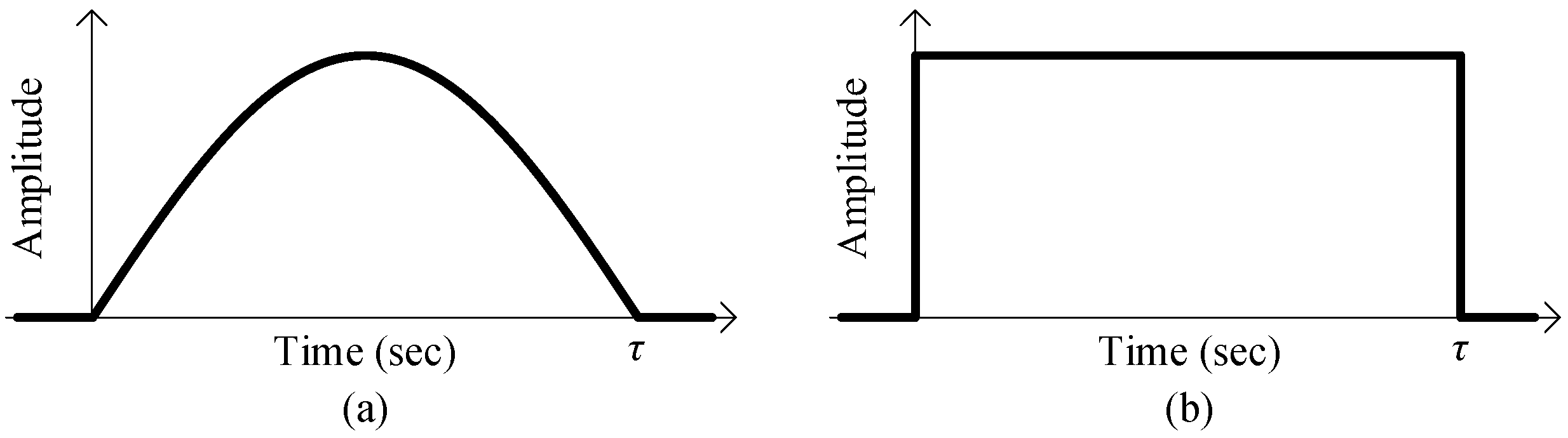
Unlike conventional polynomial-based profiles (e.g., trapezoidal velocity or S-curve profiles) that utilize rectangular pulse basis functions—resulting in discontinuities at segment switching instants—time-shifted sine-function-based basis function ensures highly smooth transitions in the time domain, as illustrated in Figure 1. This characteristic effectively suppresses high-frequency components in the reference command, thereby preventing the excitation of high-frequency vibration modes and offering significant potential for reducing residual vibrations. Furthermore, trigonometric functions possess a closure property, meaning they maintain their functional form under differentiation and integration. This allows the same mathematical algorithm to be applied systematically to derive generalized n th -order profiles, regardless of the chosen order.
Step 2.
Generate Remaining Profiles via Integration/Differentiation Chain
Once the basis functions and segment structure are defined, the remaining motion profile components (position, velocity, acceleration, jerk, etc.) are generated sequentially through a chain of integration and differentiation. Calculus is performed on the basis functions defined for each segment, while integration constants are meticulously determined to ensure that the boundary values—such as position, velocity, and acceleration—match between segments. This process ensures that the motion profile, although defined piecewise, maintains global continuity across the entire trajectory. This generative approach can be consistently applied even as the order increases and the number of segments grows, providing excellent versatility and scalability in design.
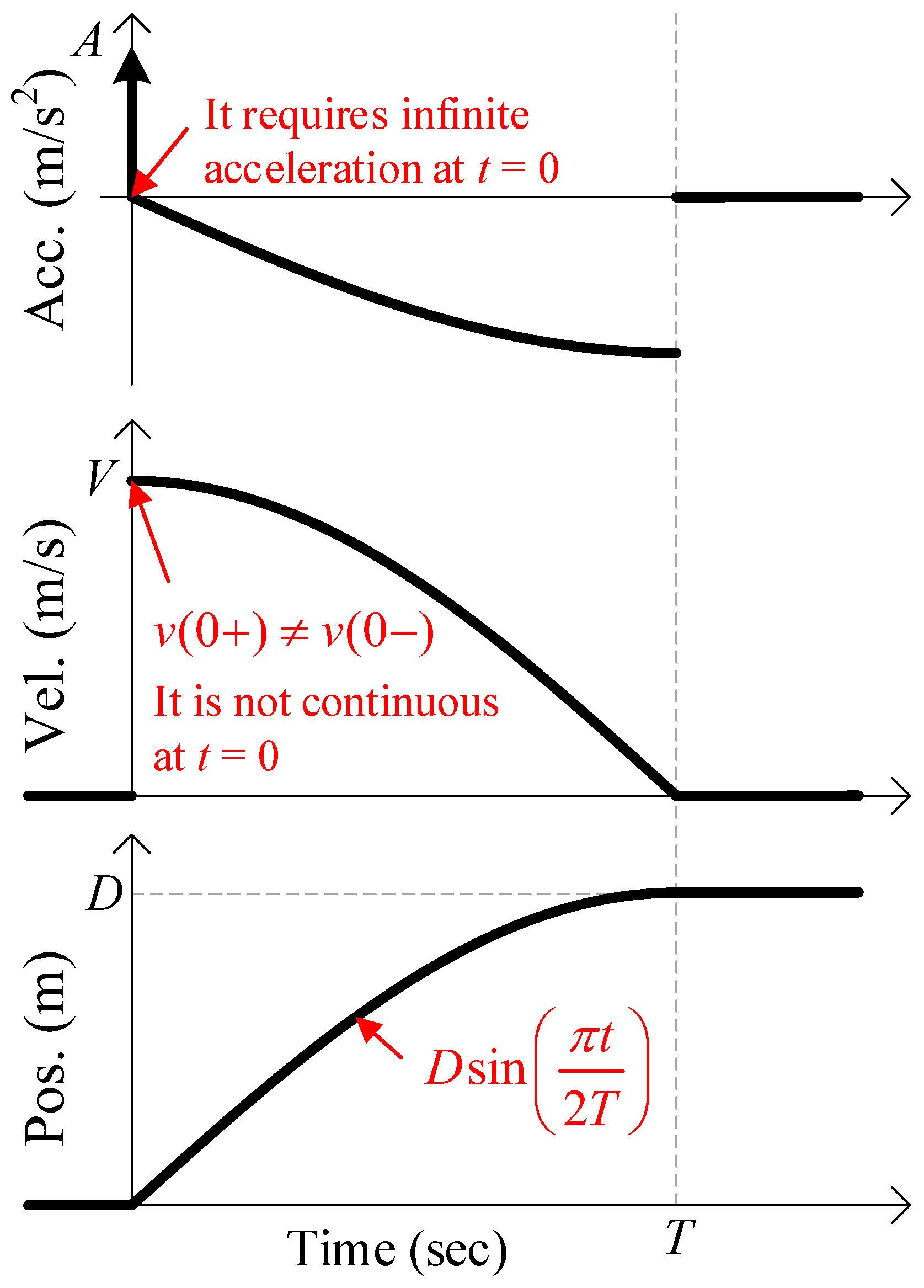
Among the various time-shifted sine motion profiles, one might consider defining the position profile directly using a time-shifted sine function as the simplest and lowest-order approach, as illustrated in Figure 2.
x ( t ) = D sin π t 2 T , 0 t T
While this position profile satisfies the displacement boundary conditions ( x ( 0 ) = 0 and x ( T ) = D ) and seemingly provides a smooth trajectory, its velocity profile is discontinuous at t = 0 . This discontinuity implies a requirement for an unrealistically large—theoretically infinite—acceleration and actuation force at the onset of motion. Consequently, given the physical limitations of actuators, the time-shifted sine position profile is physically unrealizable and is therefore excluded from the scope of this study.

3.1. Time-Shifted Sine Velocity Profile (1st-Order)

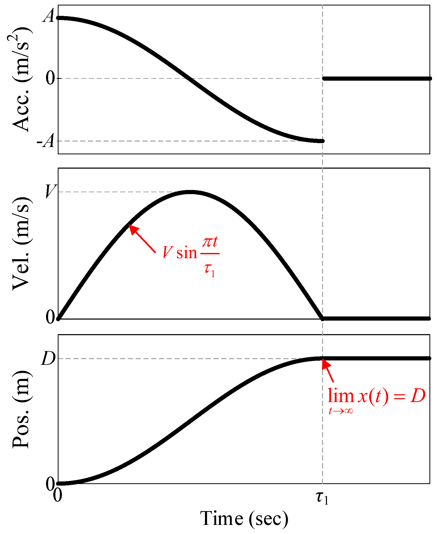
The 1st-order time-shifted sine motion profile is defined by directly prescribing the velocity trajectory using a basis function. The velocity profile is defined as:
v ( t ) = V sin π t τ 1 , 0 t T
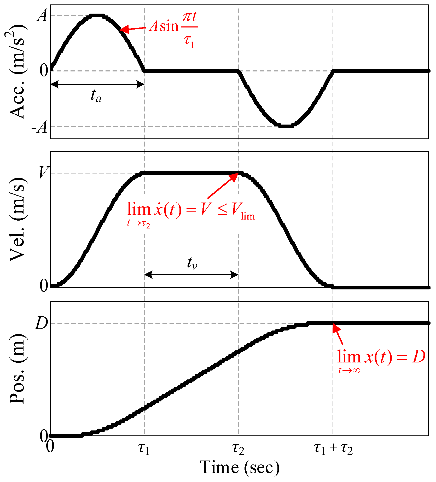
where V > 0 denotes the applied velocity amplitude and τ 1 > 0 is the duration of the sinusoidal velocity period. In this profile, the basis function is applied to the velocity command, and the remaining motion profiles are generated by differentiation and integration. As shown in Figure 3, v ( t ) is continuous and bounded over the entire motion interval. The maximum velocity max | v ( t ) | = V occurs at t = τ 1 / 2 .
The acceleration profile is obtained by differentiating v ( t ) with respect to time:
a ( t ) = V π τ 1 cos π t τ 1 , 0 t T
The acceleration profile is also bounded over the entire motion interval. The maximum acceleration max a ( t ) = A = V π τ 1 occurs at the endpoints t = 0 and t = τ 1 . Consequently, the velocity and acceleration profiles inherently satisfy the boundary conditions (C1) for the velocity and acceleration at the start and end of the motion. Furthermore, as noted in the actuator feasibility constraint (C2), the profile remains physically realizable by selecting appropriate values for V and τ 1 that do not exceed the limits V lim and A lim .
The position profile is obtained by integrating the velocity trajectory:
x ( t ) = V τ 1 π 1 cos π t τ 1 , 0 t T .
The travel displacement at t = τ 1 becomes D = x ( τ 1 ) = 2 V τ 1 π . Hence, the moving distance D is uniquely determined by the velocity amplitude V and the segment duration τ 1 . To satisfy the displacement boundary condition in C1 (i.e., x ( t ) = D for t > τ 1 ), the velocity amplitude V and the duration τ 1 must be appropriately selected to satisfy the algebraic relationship D = x ( τ 1 ) = 2 V τ 1 π .
The above time-domain derivation can be reformulated in the Laplace domain, which provides a compact and systematic way to relate motion variables without explicitly performing differentiation or integration. The Laplace transform of velocity profile is as follows:
s X ( s ) = V ω s s 2 + ω s 2 1 + e τ 1 s , where ω s = π τ 1 .
The travel displacement D can be obtained using the final value theorem, which enables direct computation of the moving distance from X ( s ) without evaluating the integral in the time domain. As a result, the relationship between D, V, and τ 1 can be derived in a straightforward manner.
lim t x ( t ) = lim s 0 s X ( s ) = lim s 0 V ω s s 2 + ω s 2 1 + e τ 1 s = 2 V ω s = 2 V τ 1 π = D
Collecting the above results, the time-shifted sine velocity profile yields the following closed-form design constraints:
D = x ( τ 1 ) = 2 V τ 1 π
V = π D 2 τ 1 V lim
A = π V τ 1 = π 2 D 2 τ 1 2 A lim
τ 1 > 0 .

3.2. Time-Shifted Sine Acceleration Profile (2nd-Order)

The 2nd-order time-shifted sine motion profile is constructed by directly prescribing the acceleration command using a sinusoidal basis function. As illustrated in Figure 4, the complete profile consists of three segments: a sinusoidal acceleration period, a constant velocity period, and a sinusoidal deceleration period. The total duration of the motion profile is T = τ 1 + τ 2 . The acceleration profile for each segment is defined as
a ( t ) = A sin π t τ 1 , 0 t τ 1 , 0 , τ 1 t τ 2 , A sin π ( t τ 2 ) τ 1 , τ 2 t τ 1 + τ 2
where A > 0 denotes the applied acceleration amplitude and τ 1 > 0 is the duration of the sinusoidal acceleration period. The velocity and position profiles can be derived by sequentially integrating the acceleration profile in each segment. To ensure global continuity across the trajectory, integration constants are determined at each segment boundary.
The velocity profile is obtained by integrating a ( t ) with v ( 0 ) = 0
v ( t ) = A τ 1 π 1 cos π t τ 1 , 0 t τ 1 , 2 A τ 1 π , τ 1 t τ 2 , A τ 1 π 1 + cos π ( t τ 2 ) τ 1 , τ 2 t τ 1 + τ 2
whose maximum value V = v ( τ 1 ) = 2 A τ 1 π occurs at t = τ 1 .
The position profile is obtained by integrating v ( t ) with x ( 0 ) = 0
x ( t ) = A τ 1 π t τ 1 π sin π t τ 1 , 0 t τ 1 , A τ 1 2 π + 2 A τ 1 π ( t τ 1 ) , τ 1 t τ 2 , A τ 1 π ( 2 τ 2 τ 1 ) + A τ 1 π ( t τ 2 ) + τ 1 π sin π ( t τ 2 ) τ 1 , τ 2 t τ 1 + τ 2 .
Accordingly, the moving distance at t = τ 1 + τ 2 becomes D = x τ 1 + τ 2 = 2 A τ 1 τ 2 π . Similar to the 1st-order case, to satisfy the displacement boundary condition in C1 (i.e., x ( t ) = D for t > T ), the design parameters A , τ 1 , and τ 2 must be appropriately selected to satisfy the above algebraic relationship.
The relationship between these motion variables can be derived more systematically in the Laplace domain. The Laplace transform of the acceleration profile is given by:
s 2 X ( s ) = A ω s s 2 + ω s 2 1 + e τ 1 s 1 e τ 2 s , where ω s = π τ 1 .
The travel displacement D can be obtained using the final value theorem and L’Hôpital’s rule.
lim t x ( t ) = lim s 0 s X ( s ) = lim s 0 A ω s s 2 + ω s 2 1 + e τ 1 s 1 e τ 2 s s = 2 A τ 2 ω s = 2 A τ 1 τ 2 π = D .
And the maximum velocity V can be obtained using final value theorem and a partial velocity profile from the motion start to the end of the constant velocity period.
lim t d x ( t ) d t = lim s 0 s 2 X ( s ) = lim s 0 A ω s s 2 + ω s 2 1 + e τ 1 s = 2 A ω s = 2 A τ 1 π = V V lim
where d x ( t ) d t = d x ( t ) d t , 0 t τ 2 , V , t > τ 2 . and s 2 X ( s ) = A ω s s 2 + ω s 2 1 + e τ 1 s .
Collecting the above results, the time-shifted sine acceleration profile yields the following closed-form design constraints:
2 A τ 1 τ 2 π = D
V = 2 A τ 1 π = D τ 2 V lim
A = π D 2 τ 1 τ 2 A lim
τ 2 τ 1 > 0 .

3.3. Time-Shifted Sine Jerk Profile (3rd-Order)

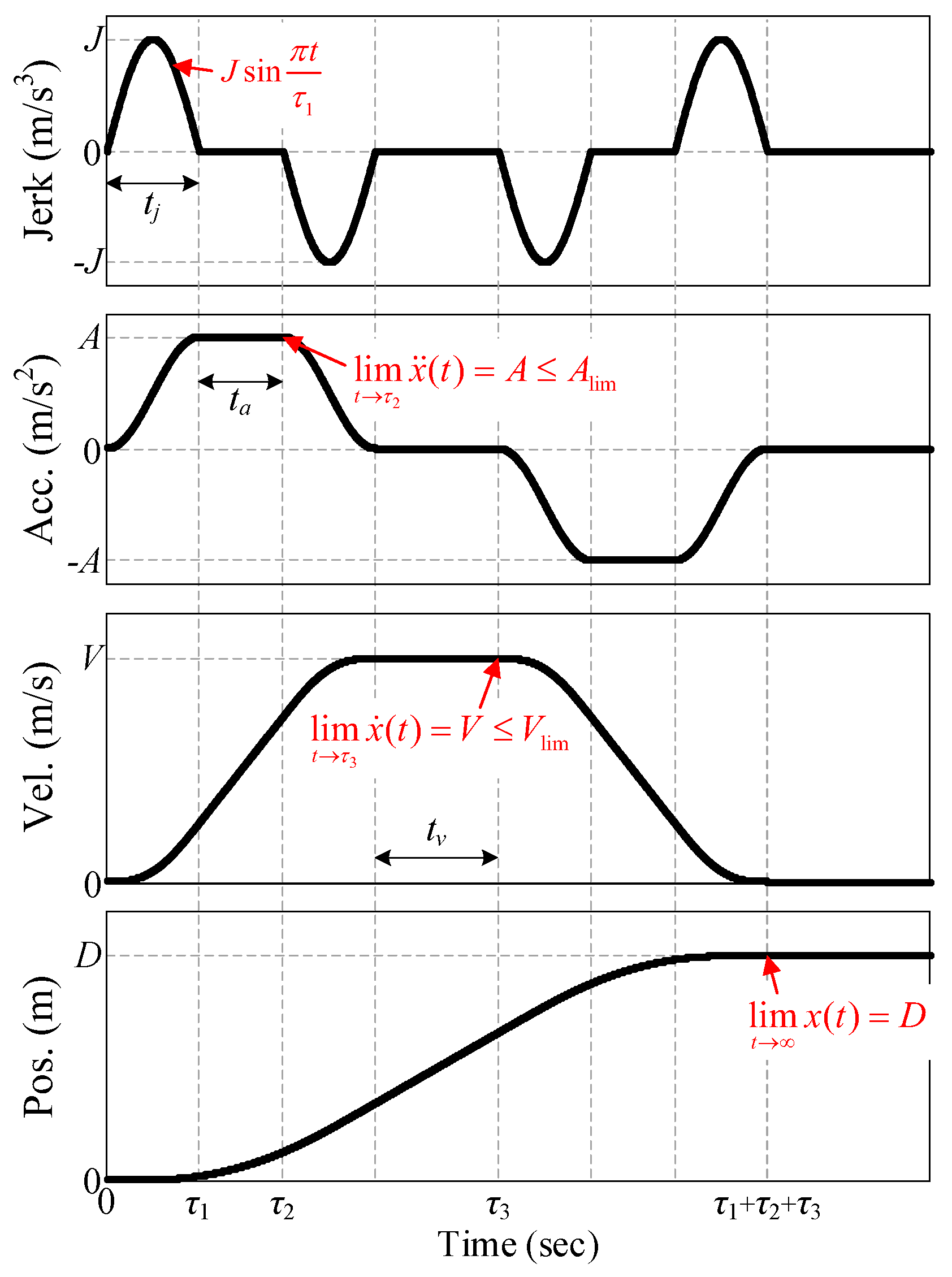
The 3rd-order time-shifted sine motion profile is constructed by directly prescribing the jerk command using a sinusoidal basis function as illustrated in Figure 5. As the order n increases to 3, the motion trajectory is divided into 2 3 1 = 7 segments, consisting of four sinusoidal jerk periods, two constant acceleration/deceleration periods, and one constant velocity period. The total duration of the motion profile is T = τ 1 + τ 2 + τ 3 . The jerk profile for each segment is defined as
j ( t ) = J sin π t τ 1 , 0 t τ 1 , 0 , τ 1 t τ 2 , J sin π ( t τ 2 ) τ 1 , τ 2 t τ 1 + τ 2 , 0 , τ 1 + τ 2 t τ 3 , J sin π ( t τ 3 ) τ 1 , τ 3 t τ 1 + τ 3 , 0 , τ 1 + τ 3 t τ 2 + τ 3 , J sin π ( t τ 2 τ 3 ) τ 1 , τ 2 + τ 3 t τ 1 + τ 2 + τ 3
where J > 0 denotes the applied jerk amplitude and τ 1 > 0 is the duration of the sinusoidal jerk period. The acceleration, velocity and position profiles can be derived by sequentially integrating the jerk profile in each segment, with the integration constants chosen to ensure continuity at the segment boundaries. The acceleration profile is obtained by integrating j ( t ) with a ( 0 ) = 0
a ( t ) = J τ 1 π 1 cos π t τ 1 , 0 t τ 1 , 2 J τ 1 π , τ 1 t τ 2 , J τ 1 π 1 + cos π ( t τ 2 ) τ 1 , τ 2 t τ 1 + τ 2 , 0 , τ 1 + τ 2 t τ 3 , J τ 1 π 1 cos π ( t τ 3 ) τ 1 , τ 3 t τ 1 + τ 3 , 2 J τ 1 π , τ 1 + τ 3 t τ 2 + τ 3 , J τ 1 π 1 + cos π ( t τ 2 τ 3 ) τ 1 , τ 2 + τ 3 t τ 1 + τ 2 + τ 3
whose maximum value A = a ( τ 1 ) = 2 J τ 1 π occurs at t = τ 1 . The velocity profile is obtained by integrating a ( t ) with v ( 0 ) = 0 .
v ( t ) = J τ 1 π t τ 1 π sin π t τ 1 , 0 t τ 1 , J τ 1 2 π + 2 J τ 1 π ( t τ 1 ) , τ 1 t τ 2 , J τ 1 π ( 2 τ 2 τ 1 ) + J τ 1 π ( t τ 2 ) + τ 1 π sin π ( t τ 2 ) τ 1 , τ 2 t τ 1 + τ 2 , 2 J τ 1 τ 2 π , τ 1 + τ 2 t τ 3 , 2 J τ 1 τ 2 π J τ 1 π ( t τ 3 ) τ 1 π sin π ( t τ 3 ) τ 1 , τ 3 t τ 1 + τ 3 , J τ 1 π ( 2 τ 2 τ 1 ) 2 J τ 1 π t τ 1 τ 3 , τ 1 + τ 3 t τ 2 + τ 3 , J τ 1 2 π J τ 1 π ( t τ 2 τ 3 ) + τ 1 π sin π ( t τ 2 τ 3 ) τ 1 , τ 2 + τ 3 t τ 1 + τ 2 + τ 3
whose maximum value V = v ( τ 1 + τ 2 ) = 2 J τ 1 τ 2 π occurs at t = τ 1 + τ 2 . The position profile is obtained by integrating v ( t ) with x ( 0 ) = 0
x ( t ) = J τ 1 π 1 2 t 2 τ 1 2 π 2 1 cos π t τ 1 , 0 t τ 1 , 2 J τ 1 3 π 1 4 1 π 2 + J τ 1 2 π ( t τ 1 ) + J τ 1 π ( t τ 1 ) 2 , τ 1 t τ 2 , 2 J τ 1 3 π 1 4 1 2 π 2 + J τ 1 2 π ( τ 2 τ 1 ) + J τ 1 π ( τ 2 τ 1 ) 2 + J τ 1 π ( 2 τ 2 τ 1 ) ( t τ 2 ) + J τ 1 π 1 2 ( t τ 2 ) 2 τ 1 2 π 2 cos π ( t τ 2 ) τ 1 , τ 2 t τ 1 + τ 2 , J τ 1 τ 2 π ( τ 1 + τ 2 ) + 2 J τ 1 τ 2 π t τ 1 τ 2 , τ 1 + τ 2 t τ 3 , J τ 1 τ 2 π ( τ 1 + τ 2 ) + 2 J τ 1 τ 2 π τ 3 τ 1 τ 2 + J τ 1 3 π 3 + 2 J τ 1 τ 2 π t τ 3 J τ 1 π 1 2 ( t τ 3 ) 2 + τ 1 2 π 2 cos π ( t τ 3 ) τ 1 , τ 3 t τ 1 + τ 3 , J τ 1 τ 2 π ( τ 1 τ 2 + 2 τ 3 ) 2 J τ 1 3 π 1 4 1 π 2 + J τ 1 π ( 2 τ 2 τ 1 ) ( t τ 1 τ 3 ) J τ 1 π ( t τ 1 τ 3 ) 2 τ 1 + τ 3 t τ 2 + τ 3 , 2 J τ 1 τ 2 τ 3 π 2 J τ 1 3 π 1 4 1 2 π 2 + J τ 1 2 π ( t τ 2 τ 3 ) J τ 1 π 1 2 ( t τ 2 τ 3 ) 2 τ 1 2 π 2 cos π ( t τ 2 τ 3 ) τ 1 , τ 2 + τ 3 t τ 1 + τ 2 + τ 3 .
Accordingly, the moving distance at t = τ 1 + τ 2 + τ 3 becomes D = x τ 1 + τ 2 + τ 3 = 2 J τ 1 τ 2 τ 3 π .
As the profile order increases, the required sequential integrations become significantly complex, making it progressively more difficult to derive relationships among the moving distance, the maximum velocity and acceleration, the magnitude of the applied basis function (e.g., J), and the representative segment durations (e.g., τ 1 , τ 2 , τ 3 , ⋯). To overcome this, the Laplace-domain formulation provides a systematic and compact alternative, allowing these relationships to be derived directly without explicitly performing repeated time-domain differentiation or integration.
The Laplace transform of jerk profile is as follows.
s 3 X ( s ) = J ω s s 2 + ω s 2 1 + e τ 1 s 1 e τ 2 s 1 e τ 3 s , where ω s = π τ 1
The travel displacement D can be obtained using the final value theorem and L’Hôpital’s rule.
lim t x ( t ) = lim s 0 s X ( s ) = lim s 0 J ω s s 2 + ω s 2 1 + e τ 1 s 1 e τ 2 s s 1 e τ 3 s s = 2 J τ 2 τ 3 ω s = 2 J τ 1 τ 2 τ 3 π = D
The maximum velocity V can be obtained by using partial velocity profile from the motion start to the end of the constant velocity period τ 3 .
lim t d x ( t ) d t = lim s 0 s 2 X ( s ) = lim s 0 J ω s s 2 + ω s 2 1 + e τ 1 s 1 e τ 2 s s = 2 J τ 2 ω s = 2 J τ 1 τ 2 π = V V lim
where d x ( t ) d t = d x ( t ) d t , 0 t τ 3 , V , t > τ 3 . and s 2 X ( s ) = J ω s s 2 + ω s 2 1 + e τ 1 s 1 e τ 2 s s .
The maximum acceleration A can be obtained by using partial acceleration profile from the motion start to the end of the constant acceleration period τ 2 .
lim t d 2 x ( t ) d t 2 = lim s 0 s 3 X ( s ) = lim s 0 J ω s s 2 + ω s 2 1 + e τ 1 s = 2 J ω s = 2 J τ 1 π = A A lim
where d 2 x ( t ) d t 2 = d 2 x ( t ) d t 2 , 0 t τ 2 , A , t > τ 2 . and s 3 X ( s ) = J ω s s 2 + ω s 2 1 + e τ 1 s .
Collecting the above results, the time-shifted sine jerk profile yields the following closed-form design constraints:
2 J τ 1 τ 2 τ 3 π = D
V = 2 J τ 1 τ 2 π = D τ 3 V lim
A = 2 J τ 1 π = D τ 2 τ 3 A lim
τ 2 τ 1 > 0 , τ 3 τ 1 + τ 2 .

3.4. n t h -Order Time-Shifted Sine Profile

The systematic derivation presented in the previous sections can be extended to an arbitrary order n, providing a unified framework for generating high-order smooth motion profiles. For an n th -order profile, the time-shifted sine basis function is assigned to the n th derivative of the position signal. The total number of segments is determined as 2 n 1 , and the total motion duration T is defined by the sum of the time parameters assigned to each derivative level. The remaining profiles are then generated by sequential integration, with integration constants chosen to ensure continuity across segment boundaries.
The Laplace-domain representation of generalized n th -order time-shifted sine profile with n 3 can be expressed as
s X ( s ) = α ω s s 2 + ω s 2 1 + e τ 1 s i = 2 n 1 e τ i s s , where ω s = π τ 1
where α denotes the maximum magnitude of the n th derivative of the position profile, and τ i is a fundamental time parameter for the sine basis function. All time parameters should satisfy the feasibility conditions imposed by the segment structure (i.e., τ 1 0 , τ i m = 1 i 1 τ m ).
The travel displacement D is obtained from X ( s ) using the final value theorem, where the resulting limit is evaluated via L’Hôpital’s rule to derive a closed-form relationship among D, α , and τ i .
lim t x ( t ) = lim s 0 s X ( s ) = lim s 0 α ω s s 2 + ω s 2 1 + e τ 1 s i = 2 n 1 e τ i s s = 2 α π i = 1 n τ i = D .
The maximum velocity V is determined from a partial velocity profile defined over the interval from the motion start to the end of the constant velocity period. This approach enables a compact expression for V in terms of α and τ i , where τ n 1 denotes the end time of the constant velocity period.
lim t d x ( t ) d t = lim s 0 s 2 X ( s ) = lim s 0 α ω s s 2 + ω s 2 1 + e τ 1 s i = 2 n 1 1 e τ i s s = 2 α π i = 1 n 1 τ i = V V lim
where d x ( t ) d t = d x ( t ) d t , 0 t τ n 1 , V , t > τ n 1 . and s 2 X ( s ) = α ω s s 2 + ω s 2 1 + e τ 1 s i = 2 n 1 1 e τ i s s .
Similarly, the maximum acceleration A is obtained from a partial acceleration profile defined over the interval from the motion start to the end of the constant-acceleration segment. This yields an explicit expression for A in terms of α and τ i , where τ n 2 denotes the end time of the constant-acceleration period.
lim t d 2 x ( t ) d t 2 = lim s 0 s 3 X ( s ) = lim s 0 α ω s s 2 + ω s 2 1 + e τ 1 s i = 2 n 2 1 e τ i s s = 2 α π i = 1 n 2 τ i = A A lim
where d 2 x ( t ) d t 2 = d 2 x ( t ) d t 2 , 0 t τ n 2 , A , t > τ n 2 . and s 3 X ( s ) = α ω s s 2 + ω s 2 1 + e τ 1 s i = 2 n 2 1 e τ i s s .
Collecting the above results, the n th -order time-shifted sine profile yields the following closed-form design constraints:
2 α π i = 1 n τ i = D
V = D τ n V lim
A = D τ n 1 τ n A lim
τ 1 0 , τ i m = 1 i 1 τ m .

4. Motion-Induced Vibration and Conditions for Its Suppression

4.1. Analysis of Motion-Induced Vibration

In high-speed precision positioning systems, a motion profile is not merely a reference command satisfying kinematic constraints such as moving distance, maximum velocity, and maximum acceleration; rather, it plays a crucial role in determining the magnitude of motion-induced vibration. In particular, the residual vibration that remains after the completion of motion directly degrades positioning accuracy and significantly prolongs the settling time. Therefore, it is essential to establish analytical conditions under which residual vibration is minimized.
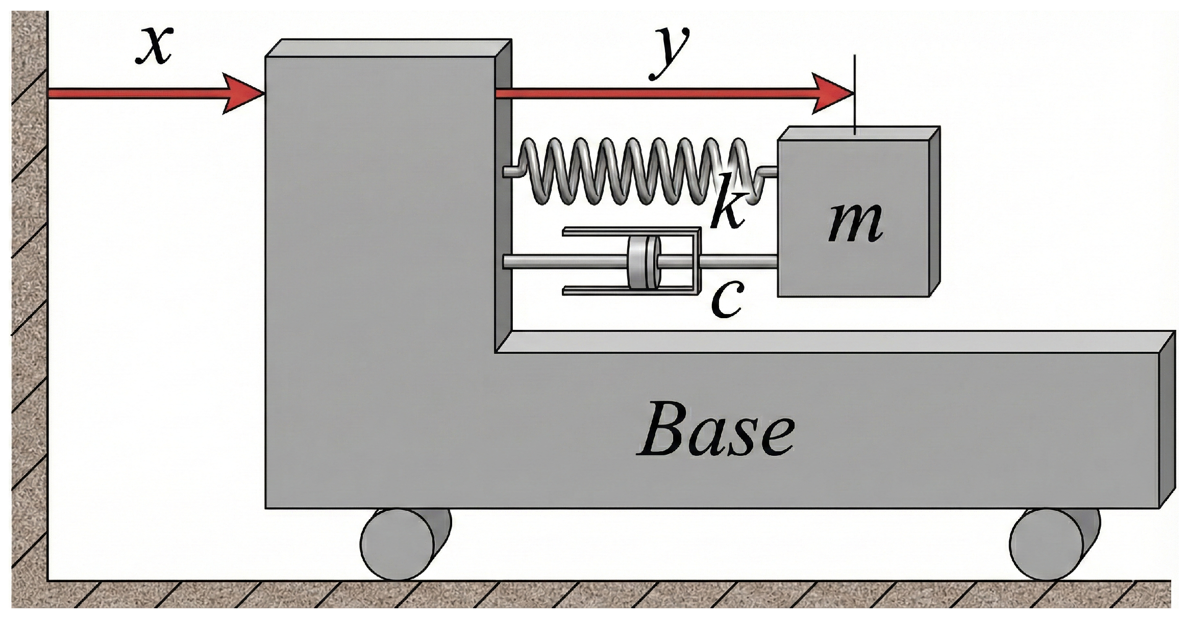
Although practical mechanical systems often exhibit complex dynamics, including multi-degree-of-freedom behavior and nonlinearities, this study employs a simplified yet fundamental single-degree-of-freedom structural model to capture the essential mechanics of residual vibration. Specifically, we consider a base-excited mass–spring–damper system mounted on a translating cart, as illustrated in Figure 6. Let x ( t ) denote the absolute displacement of the cart and y ( t ) the relative displacement of the attached mass with respect to the cart. The mass–spring–damper subsystem is excited by the cart motion. For a system with mass m, damping coefficient c, and stiffness k, the transfer function can be derived as
Y ( s ) = s 2 s 2 + 2 ζ ω n s + ω n 2 X ( s )
where ω n = k m is the natural frequency and ζ = c 2 m k is the damping ratio. This formulation indicates that motion-induced vibration is fundamentally governed by the cart motion. Consequently, the vibration level, particularly the residual vibration after motion completion, varies depending on the shape of the motion profile. This observation provides the primary motivation for designing optimized motion profiles that achieve an ideal balance between rapid point-to-point transfer and minimal residual vibration.
The correlation between the transfer function of a transport system with a flexible structure and the Laplace transform of the designed motion profile, X ( s ) , allows for the calculation of the time-domain vibration response y ( t ) . Specifically, the relative vibration displacement y ( t ) of the flexible structure, induced by the cart motion, is obtained via the inverse Laplace transform of the product of the system dynamics and the reference input profile:
y ( t ) = L 1 s 2 s 2 + 2 ζ ω n s + ω n 2 X ( s ) .
By substituting the Laplace transform X ( s ) of the 1st-order time-shifted sine motion profile, given in (8), into (45), the residual vibration response y ( t ) occurring after the motion completion time ( t > T , where T = τ 1 ) can be expressed as:
y ( t ) = L 1 s 2 s 2 + 2 ζ ω n s + ω n 2 X ( s ) = L 1 s 2 s 2 + 2 ζ ω n s + ω n 2 V s ω s s 2 + ω s 2 1 + e τ 1 s = L 1 V ω s s s 2 + 2 ζ ω n s + ω n 2 s 2 + ω s 2 i = 0 1 a i e t i s
where V denotes the velocity amplitude and ω s = π τ 1 as defined in Section 3.1. The parameters a i and t i are directly determined by the individual terms in the factor ( 1 + e τ 1 s ) as [ a 0 , a 1 ] = [ 1 , 1 ] and [ t 0 , t 1 ] = [ 0 , τ 1 ] .
To express this result in a form that is directly interpretable in the time domain, the denominator is decomposed via partial fraction expansion into an input-profile-related term characterized by ω s , and a system-dynamics-related term characterized by ω n :
y ( t ) = V ω s ω n 2 ω s 2 2 + 2 ζ ω n ω s 2 L 1 ω n 2 ω s 2 s + 2 ζ ω n ω s 2 s 2 + ω s 2 ω n 2 ω s 2 s + 2 ζ ω n 3 s 2 + 2 ζ ω n s + ω n 2 i = 0 1 a i e t i s .
First, we perform the inverse Laplace transform of the leading term, which contains the input-profile frequency component ω s and represents the forced response induced by the motion profile shape. Under appropriately designed time-shift conditions, this forced component vanishes for t > T , as shown below:
L 1 ( ω n 2 ω s 2 ) s + 2 ζ ω n ω s 2 s 2 + ω s 2 i = 0 1 a i e t i s = ( ω n 2 ω s 2 ) L 1 s s 2 + ω s 2 i = 0 1 a i e t i s + 2 ζ ω n ω s L 1 ω s s 2 + ω s 2 i = 0 1 a i e t i s = ( ω n 2 ω s 2 ) i = 0 1 a i cos ω s ( t t i ) u ( t t i ) + 2 ζ ω n ω s i = 0 1 a i sin ω s ( t t i ) u ( t t i ) . = t > T ( ω n 2 ω s 2 ) i = 0 1 a i cos ω s ( t t i ) + 2 ζ ω n ω s i = 0 1 a i sin ω s ( t t i ) = 0
where u ( t t i ) is the unit step function defined as u ( t t i ) = 1 for t t i and u ( t t i ) = 0 for t < t i . Because cos ω s t + cos ω s t π = 0 and s i n ω s t + sin ω s t π = 0 , the forced-response term in (48) cancels identically for t > T .
Subsequently, the inverse Laplace transform is performed on the trailing term, which contains the system’s natural frequency ( ω n ) and damping ratio ( ζ ). This component captures the physical characteristics of the transient response generated by the excitation of the system’s flexible mode:
L 1 ω n 2 ω s 2 s + 2 ζ ω n 3 s 2 + 2 ζ ω n s + ω n 2 i = 0 1 a i e t i s = L 1 ω n 2 ω s 2 s + ζ ω n ( s + ζ ω n ) 2 + ω n 2 ( 1 ζ 2 ) i = 0 1 a i e t i s L 1 ζ ω n ω s 2 + ζ ω n 3 ( s + ζ ω n ) 2 + ω n 2 ( 1 ζ 2 ) i = 0 1 a i e t i s = t > T ω n 2 ω s 2 i = 0 1 a i e ζ ω n ( t t i ) cos ω d ( t t i ) ζ ω n ( ω s 2 + ω n 2 ) ω d i = 0 1 a i e ζ ω n ( t t i ) sin ω d ( t t i ) = i = 0 1 a i e ζ ω n ( t t i ) ω n 2 ω s 2 2 + 2 ζ ω n ω s 2 1 ζ 2 sin ω d t ω d t i + ϕ
where ω d = ω n 1 ζ 2 , sin ϕ = Ψ 1 Ψ 1 2 + Ψ 2 2 , Ψ 1 = ω n 2 ω s 2 , and Ψ 2 = ζ ω n ( ω s 2 + ω n 2 ) ω d .
Finally, the complete time-domain vibration response y ( t ) is obtained by combining the two components derived above.
y ( t > T ) = V e ζ ω n t 1 ζ 2 ω s ω n 2 ω s 2 2 + 2 ζ ω n ω s 2 i = 0 1 a i e ζ ω n t i sin ω d t ω d t i + ϕ
By relating the vibration response function y ( t ) to the pole locations s = s p ( = ζ ω n ± j ω d ) in the complex plane, a fundamental result is obtained: the residual vibration amplitude is proportional to the magnitude of the motion profile’s Laplace transform evaluated at the system’s complex poles, s = s p , as shown below.
y ( t > T ) = V e ζ ω n t 1 ζ 2 ω s ω n 2 ω s 2 2 + 2 ζ ω n ω s 2 i = 0 1 a i e ζ ω n t i sin ω d t ω d t i + ϕ = V e ζ ω n t 1 ζ 2 ω s ω n 2 ω s 2 2 + 2 ζ ω n ω s 2 Ψ C 2 + Ψ S 2 sin ω d t + ϕ φ = V e ζ ω n t 1 ζ 2 ω s s 2 + ω s 2 s = s p i = 0 1 a i e t i s s = s p sin ω d t + ϕ φ
where Ψ C = i = 0 1 a i e ζ ω n t i cos ( ω d t i ) , Ψ S = i = 0 1 a i e ζ ω n t i sin ( ω d t i ) , and cos φ = Ψ C Ψ C 2 + Ψ S 2 . To clarify the residual vibration characteristics after motion completion ( t > T ), we derive the envelope function y envelope ( t ) , which defines the peak amplitude bounds of the vibration by omitting the harmonic terms. This function quantitatively characterizes the vibration decay envelope and the maximum amplitude over time, as follows:
y envelope ( t > T ) = e ζ ω n t 1 ζ 2 V ω s s 2 + ω s 2 s = s p i = 0 1 a i e t i s s = s p = e ζ ω n t 1 ζ 2 s X ( s ) s = s p = ω n e ζ ω n t 1 ζ 2 X ( s ) s = s p .
Following the derivation in (52), it is demonstrated that the residual vibration amplitude is directly proportional to the magnitude of the motion profile’s Laplace transform evaluated at the system’s complex poles ( s = s p ). Similarly, it can be demonstrated through a consistent derivation process that the same relationship holds true for higher-order profiles, such as the time-shifted sine acceleration ( n = 2 ) and jerk ( n = 3 ) profiles.
Furthermore, by differentiating the vibration response function y ( t ) and rearranging the terms, it can be demonstrated that the amplitudes of the velocity and acceleration responses are also proportional to X ( s ) s = s p . This relationship can be expressed through the envelope functions for the velocity and acceleration responses, v envelope ( t ) and a envelope ( t ) , as follows:
v envelope ( t > T ) = ω n 2 e ζ ω n t 1 ζ 2 X ( s ) s = s p a envelope ( t > T ) = ω n 3 e ζ ω n t 1 ζ 2 X ( s ) s = s p .

4.2. Condition for Minimized Residual Vibration

The result obtained in Section 4.1 indicates that the residual vibration amplitude is proportional to the magnitude | X ( s p ) | . In the context of the proposed time-shifted sine motion profiles, the primary design objective for minimizing vibration during motion is to strategically select the time parameters τ i such that | X ( s p ) | is minimized. The following subsections describe the criteria for selecting these time parameters to achieve optimal vibration suppression for each profile order.

4.2.1. Time-Shifted Sine Velocity Profile (1st-Order)

By substituting (8) and (10) into (52), the envelope of the residual vibration response for t > T is expressed as:
y envelope ( t > T ) = π D e ζ ω n t 2 1 ζ 2 ω s s 2 + ω s 2 s = s p 1 + e s τ 1 s = s p τ 1 .
Given the fundamental relationship ω s = π τ 1 , Equation (54) reveals that the residual vibration envelope is effectively reduced to a single-variable function of the time parameter τ 1 . To facilitate the minimization of this function, it is beneficial to interpret y envelope as the product of two distinct components: the Sinusoidal Term and the Impulse Term.
y envelope ω s s 2 + ω s 2 s = s p Sinusoidal Term × 1 + e s τ 1 s = s p τ 1 Impulse Term .
For a system with negligible damping ( ζ 0 ), the complex poles can be approximated as s p j ω n . Under this condition, the first step in minimizing the residual vibration magnitude is to identify the conditions under which the numerator of the Impulse Term vanishes, i.e., 1 + e j ω n τ 1 = 0 . This condition is satisfied when the phase angle ω n τ 1 is an odd multiple of π , yielding the candidate solutions τ 1 = ( k + 1 2 ) T d for k = 0 , 1 , 2 , , where the natural period is defined as T d = 2 π ω d .
However, a critical resonance singularity arises at the smallest candidate solution where k = 0 , corresponding to τ 1 = 0.5 T d . In this specific case, the angular frequency of the motion profile matches the system’s natural frequency ( ω s = ω n ). Consequently, the denominator | s 2 + ω s 2 | within the Sinusoidal Term approaches zero, resulting in an indeterminate form of 0 0 in the envelope function. By applying L’Hôpital’s rule to evaluate the limit at this point, it can be demonstrated that the vibration amplitude converges to a finite, non-zero value.
As a result, the residual vibration for an undamped system is effectively minimized when the duration satisfies the following condition:
τ 1 = k + 1 2 T d , k = 1 , 2 , 3 , .
This indicates that the motion duration must be at least 1.5 times the damped natural period to achieve a true null in the residual vibration response.
Similarly, for underdamped systems where 0 < ζ < 1 , the minimization of the Impulse Term follows a comparable approach, as it is primarily governed by its numerator, 1 + e s τ 1 s = s p . By substituting the system pole s p = ζ ω n + j ω d , this term can be explicitly expanded as:
1 + e ( ζ ω n + j ω d ) τ 1 = 1 + e ζ ω n τ 1 e j ω d τ 1 .
To minimize this magnitude, the rotating complex vector e j ω d τ 1 must align in opposition to the unity vector, thereby creating destructive interference. The condition for this phase alignment is satisfied when:
e j ω d τ 1 = ω d τ 1 = ( 2 k + 1 ) π , k = 0 , 1 , 2 , .
However, the shortest candidate duration where k = 0 ( τ 1 = 0.5 T d ) leads to a critical issue within the Sinusoidal Term. At this duration, the excitation frequency becomes ω s = π τ 1 = ω d . Since the excitation frequency ω s coincides with the damped natural frequency, the Sinusoidal Term undergoes resonance amplification. This resonance effectively offsets the vibration suppression provided by the Impulse Term, rendering the k = 0 case invalid for the minimum vibration condition. Consequently, even for underdamped systems ( ζ 0 ), the residual vibration is minimized only when the duration satisfies the condition previously established in (56).
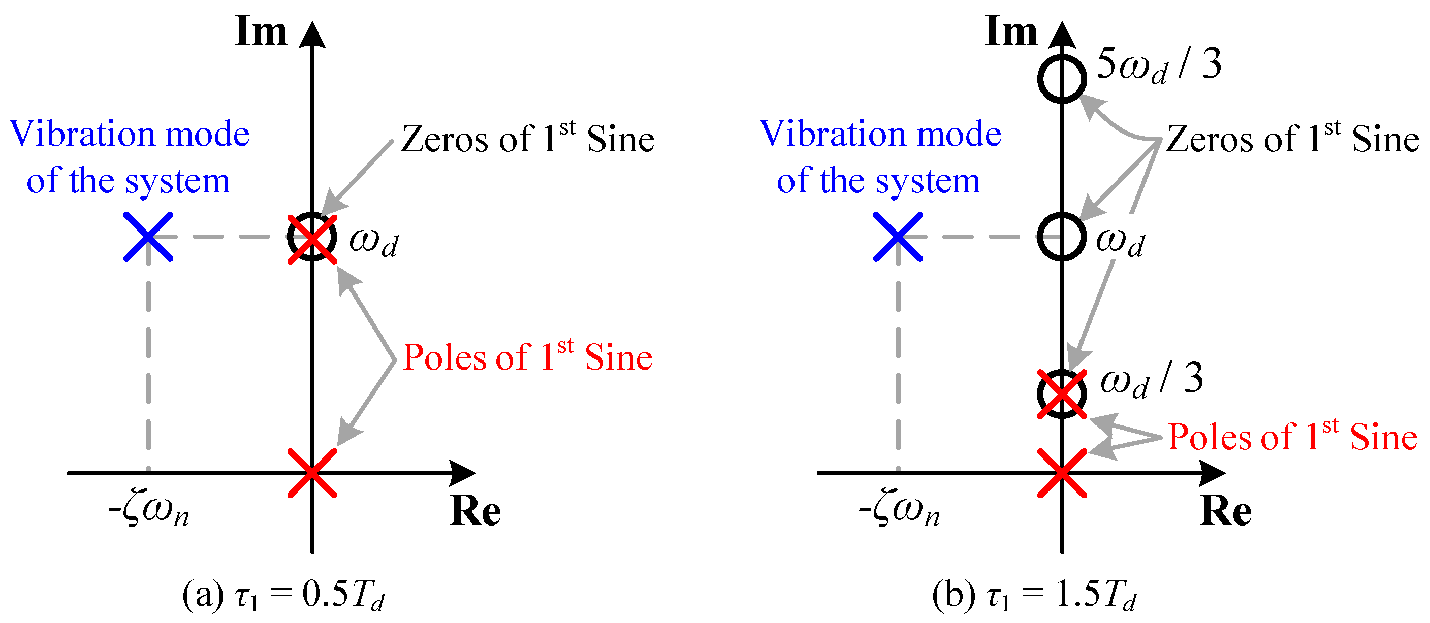
The validity of these conditions can be also examined through the perspective of pole-zero cancellation in the complex s-plane as illustrated in Figure 7. The Laplace transform of the velocity profile comprises input poles from the Sinusoidal Term and zeros from the Impulse Term. As shown in Figure 7a, at the shortest duration candidate where k = 0 ( τ 1 = 0.5 T d ), the Impulse Term places its zeros nearest to the system poles to suppress vibration. However, the Sinusoidal Term simultaneously places input poles at the same frequency ( ω s ω d ). Consequently, the input poles of the Sinusoidal Term cancel the zeros of the Impulse Term, thereby preventing these zeros from effectively suppressing the system’s vibration poles.
In contrast, as depicted in Figure 7b, for cases where k 1 (corresponding to τ 1 = 1.5 T d , 2.5 T d , ), the poles from the Sinusoidal term are shifted to lower frequencies defined by ω s = ω d 2 k + 1 , effectively moving them far away from the system poles. Meanwhile, the zeros of the Impulse Term remain optimally positioned to cancel the system poles. This separation allows the zero-placement strategy to function without interference. Specifically, for the undamped case ( ζ = 0 ), the zeros of the Impulse Term perfectly cancel the system’s vibration poles, resulting in theoretically zero residual vibration. Similarly, for underdamped systems ( ζ 0 ), this separation enables the zeros to neutralize the system’s oscillatory dynamics, thereby achieving minimization of residual vibration.

4.2.2. n t h -Order Time-Shifted Sine Profile

Extending the analysis to the general n-th order case, the residual vibration envelope is derived by incorporating the additional convolution stages. Based on the updated formulation, the envelope function is proportional to the product of the Sinusoidal Term, the Primary Impulse Term, and a sequence of Secondary Impulse Terms:
y envelope ω s s 2 + ω s 2 s = s p Sinusoidal Term × | 1 + e s τ 1 | s = s p τ 1 Primary Impulse Term × i = 2 n 1 e s τ i s = s p τ i Secondary Impulse Terms .
The optimization of τ 1 follows the same logic as the first-order case discussed in Section 4.2.1. To minimize the Primary Impulse Term while avoiding resonance in the Sinusoidal Term, τ 1 must satisfy the condition previously established in (56):
τ 1 = k + 1 2 T d , k = 1 , 2 , 3 , .
The subsequent time parameters, τ i (for i = 2 , , n ), are governed by the Secondary Impulse Terms. Unlike the primary term, these terms are characterized by the form | 1 e s τ i | . To minimize these terms, we analyze their magnitude by substituting the system pole s p = ζ ω n + j ω d , similar to the derivation in (57):
1 e s τ i s = s p = 1 e ζ ω n τ i e j ω d τ i .
In (61), the term e ζ ω n τ i represents a magnitude scaling factor, while e j ω d τ i represents the phase rotation. To minimize the total magnitude, the rotating vector e j ω d τ i must align with the real axis in the positive direction to cancel the leading unity term. This phase alignment condition is satisfied when:
e j ω d τ i = ω d τ i = 2 k i π , k i = 1 , 2 , 3 , .
This implies that the zeros of the Secondary Impulse Terms are located at integer multiples of the damped natural period ( T d ).
τ i = k i T d , k i = 1 , 2 , 3 ,
Consequently, by combining the primary condition (60) and the secondary condition (63), the n th -order profile achieves a robust zero-placement structure that effectively suppresses vibration across a broader frequency range.
Furthermore, it is important to emphasize that both the construction of the motion profiles (as described in Section 3) and the determination of their optimal parameters are achieved through explicit algebraic expressions without the need for iterative numerical optimization. While conventional trajectory optimization and realization often requires significant computational resources for real-time optimization, the proposed framework allows for the instantaneous generation of vibration-suppressed trajectories using negligible computational overhead. This efficiency makes the suggested methodology highly suitable for implementation in low-performance industrial controllers where real-time responsiveness is critical.

5. Case Study: Simulation for Long-Stroke Scenario

To address the problem of minimizing residual vibration induced by high-speed motion, it is necessary to establish an appropriate dynamic model of the transfer system. In practical industrial equipment, the actual mechanical system is governed by complex dynamics, including multiple vibration modes, structural flexibilities, coupling effects, and various nonlinear behaviors. Although such a high-fidelity model can describe the real system more accurately, it is often difficult to interpret and does not clearly reveal how the parameters of a motion profile influence vibration generation. For this reason, this study adopts a simplified representative model, as illustrated in Figure 6, in order to clearly extract the dominant physical principles and obtain meaningful insights for motion profile design. The purpose of using this simplified model is not to replicate every detail of the real system, but rather to provide a tractable framework in which the effect of motion-profile parameter tuning on residual vibration can be analyzed and understood in a transparent manner.
In the simplified model, the base represents the moving component that is directly connected to the actuator and sensor. This base is assumed to be precisely controlled such that it accurately follows a given reference trajectory, i.e., the motion profile. Therefore, the base motion can be regarded as the system input, and its displacement is denoted by X ( s ) in the Laplace domain. Attached to the base is a lumped mass–spring–damper subsystem consisting of a mass m, a spring with stiffness k, and a viscous damper with damping coefficient c. This subsystem represents the flexible mechanical parts in which motion-induced vibration occurs; in other words, it approximates the dominant vibration mode of the transfer system. When the base moves according to the commanded motion profile, the inertia of the attached mass causes it to oscillate relative to the base, producing vibration. The vibration displacement of this subsystem is denoted by Y ( s ) . Based on this representation, the relationship between the base displacement and the resulting vibration response can be expressed in the Laplace domain by the following transfer function, as shown in (44). The transfer function highlights that vibration is strongly influenced by the dynamic components of the motion profile.
The main advantage of adopting this simplified model is that it provides a clear and interpretable link between the commanded motion profile and the resulting vibration behavior. This allows the designer to systematically adjust motion-profile parameters to improve high-speed operational performance while suppressing residual vibration. Although real transfer systems may contain multiple vibration modes, the insights obtained from this single-mode approximation can be effectively extended to multi-degree-of-freedom (MDOF) systems through the principle of superposition. Therefore, the simplified modeling approach serves as a practical foundation for motion profile optimization and vibration reduction in real applications.
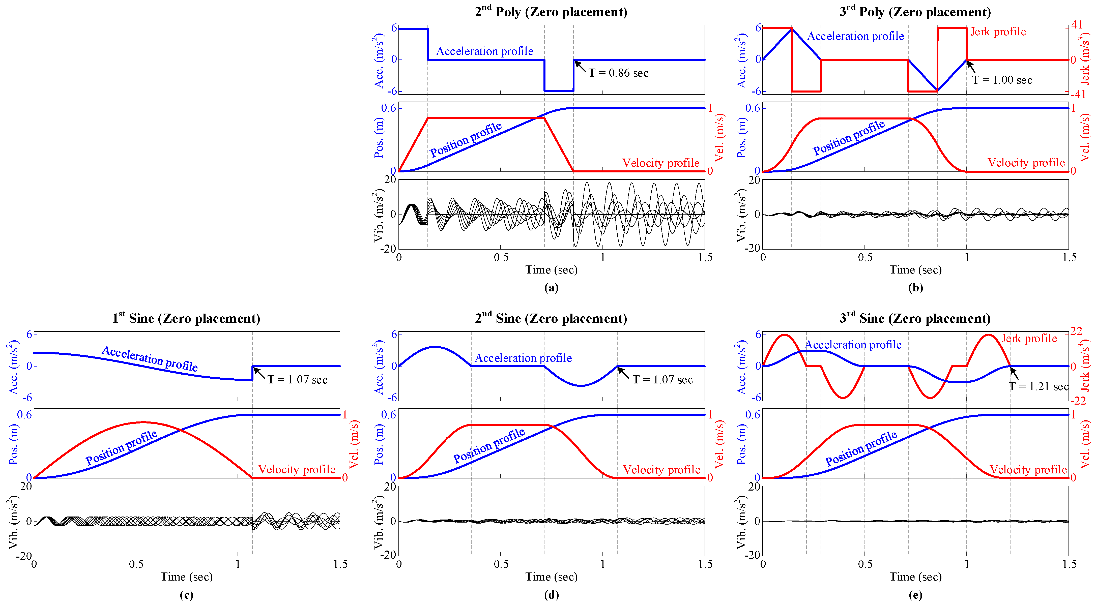
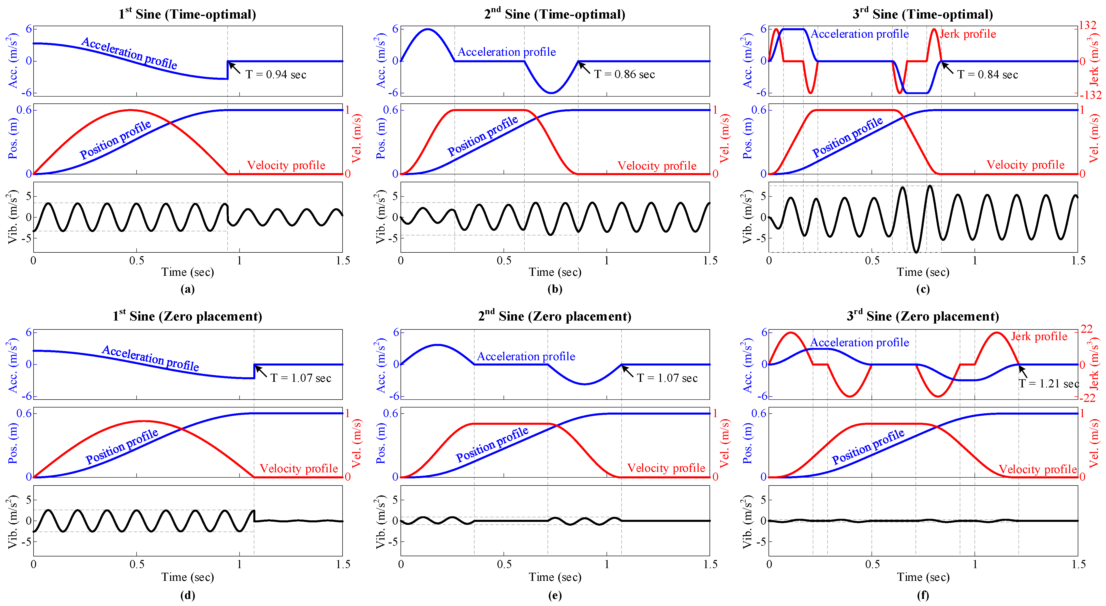
Based on this model, we investigate the proposed closed-form motion-profile design method, referred to as zero placement, applied to the time-shifted sine family, including the 1st Sine (time-shifted sine velocity profile), the 2nd Sine (time-shifted sine acceleration profile), and the 3rd Sine (time-shifted sine jerk profile), for high-speed transfer with minimal vibration excitation. By analytically determining key design parameters (e.g., τ 1 , τ 2 , τ 3 , ), the proposed method shapes the commanded trajectory such that the dominant vibration mode is barely excited, thereby enabling rapid motion with negligible residual vibration. The comparison results are presented in Figure 8, where the motion profiles designed using the conventional time-optimal strategy and those designed using the proposed zero placement strategy are shown together with the vibration response of the second mass when the base follows the corresponding trajectories.
The case study is conducted under a fixed set of physical constraints and vibration characteristics, which are summarized in Table 1: moving distance D = 0.6 m , velocity limit V lim = 1 m / s , acceleration limit A lim = 6 m / s 2 , natural frequency f n = 7 Hz , and damping ratio ζ = 0.001 . Under these conditions, the objective is to compare how the vibration amplitude of the second mass and the overall time performance change when the base motion is generated within the same velocity and acceleration constraints. This comparison is particularly important because, in many vibration-sensitive applications, the practical throughput is determined not only by the motion completion time but also by the settling behavior required for the system to become sufficiently stable after the motion ends.
Figure 8a–c illustrate the results obtained using the time-optimal approach for the 1st, 2nd, and 3rd Sine motion profiles. In this approach, the motion is designed to minimize the motion completion time by utilizing the velocity and acceleration limits as aggressively as possible, typically driving the profile such that the peak velocity and/or peak acceleration approach ( V lim , A lim ) . As expected, this strategy produces the shortest motion completion time. However, the vibration response of the second mass shows that significant residual vibration remains after the base reaches the target position. This residual vibration increases the settling time required for stabilization, indicating that although the transfer itself is fast, the total cycle time can be unfavorable when stabilization is required before subsequent operations.
Figure 8d–f present the corresponding results obtained using the proposed zero placement method for the same family of motion profiles. Unlike the time-optimal strategy, the proposed method determines the motion parameters ( τ 1 , τ 2 , τ 3 , ) in a closed-form manner to suppress both transient vibration during motion and residual vibration after arrival. Due to the vibration-oriented design objective, the resulting profiles may intentionally avoid saturating the constraints, meaning that the realized peak velocity and acceleration can be smaller than V lim and A lim , and thus the motion completion time can increase slightly. Nevertheless, the key advantage is that residual vibration is drastically reduced, and the second mass stabilizes rapidly immediately after motion completion. Consequently, when the settling behavior is included, the proposed method can provide a shorter effective cycle time despite a modest increase in pure travel time.
Table 2 quantitatively summarizes the key design parameters and performance metrics for the time-optimal and zero placement designs. As demonstrated in the table, the proposed method reduces the peak residual vibration by approximately 94.0 % for the 1st Sine profile and by 99.9 % for both the 2nd and 3rd Sine profiles compared with the time-optimal designs, confirming that near-vibration-free arrival can be achieved. In addition, the maximum transient vibration during the transfer is also reduced by 22.7 % , 76.8 % , and 96.5 % for the 1st, 2nd, and 3rd Sine profiles, respectively, indicating that the proposed approach improves not only post-motion settling behavior but also vibration performance throughout the motion.
Furthermore, the proposed zero placement method reveals a characteristic structure in the selected design parameters relative to the dominant vibration period T d = 1 f n 1 ζ 2 . Specifically, τ 1 is typically assigned as a half-integer multiple of T d (e.g., 1.5 T d , 2.5 T d , 3.5 T d , …), whereas the remaining parameters such as τ 2 , τ 3 , … are assigned as integer multiples of T d (e.g., 2 T d , 3 T d , 4 T d , …). This structure provides an intuitive physical interpretation: by aligning the timing of excitation components with the vibration period, the vibrations generated during different phases of the motion are arranged to overlap with approximately opposite phase, leading to destructive interference and cancellation of motion-induced vibration. The decision to assign the foundational time parameter τ 1 as a half-integer multiple of the natural period T d (e.g., 1.5 T d , 2.5 T d , ) is rooted in the principle of self-cancellation through destructive interference. This unique half-integer characteristic of the time-shifted sine motion profile enables robust vibration suppression and enhanced energy efficiency without requiring computationally expensive iterative numerical optimization. From a practical standpoint, such vibration minimization is critical for optimizing peak actuator energy consumption, as the total force required from the actuator is determined not only by the commanded base acceleration but also by the vibratory inertial forces generated by the attached mass. Since peak power consumption is governed by the product of instantaneous velocity and total acceleration ( P v · a t o t a l ), the reduction in these vibratory forces directly lowers the peak power demand. Consequently, this analytical approach effectively prevents actuator saturation and ensures more sustainable and reliable hardware operation.
Overall, these results demonstrate that the proposed closed-form motion-profile design approach based on zero placement provides an effective means of achieving high-speed transfer with minimal vibration excitation. While the time-optimal strategy minimizes the motion completion time by aggressively exploiting the allowable constraints, it can significantly excite the dominant vibration mode and increase the post-motion stabilization time. In contrast, the proposed approach systematically designs the motion-profile parameters to minimize both transient and residual vibrations, thereby achieving a more favorable effective cycle time in vibration-sensitive transfer systems.
Following the nominal case study described above, we further investigate the robustness of the proposed zero placement motion-profile design strategy under modeling uncertainties. The core idea of the proposed strategy is to design motion profiles such that the zeros of the designed motion profile are placed as close as possible to the vibratory poles of the system, thereby minimizing the excitation of the dominant vibration mode. In practical applications, however, the system vibration characteristics are not perfectly known and can vary due to changes in payload, structural stiffness, temperature, wear, and other uncertain factors. Therefore, even if a motion profile is appropriately designed based on nominal vibration parameters, residual vibration may reappear when the actual system deviates from the nominal model. To evaluate the robustness of the proposed strategy, we designed various motion profiles using the same zero placement approach and conducted repeated simulations while systematically varying the modeling error in the natural frequency.
Specifically, five representative motion profiles were considered in this robustness study: a trapezoidal velocity profile based on a 2nd-order polynomial (2nd Poly), an S-curve profile based on a 3rd-order polynomial (3rd Poly), a time-shifted sine velocity profile (1st Sine), a time-shifted sine acceleration profile (2nd Sine), and a time-shifted sine jerk profile (3rd Sine). Under the same displacement requirement and kinematic constraints, each motion profile was designed using the proposed zero placement strategy based on the nominal natural frequency of f n = 7 Hz . Then, the actual natural frequency was perturbed to represent modeling uncertainty, and the resulting motion-induced vibration of the second mass was observed. As shown in Figure 9, the actual natural frequency was varied by 0 % , 5 % , 10 % , 15 % , 20 % , 25 % , and 30 % relative to the nominal value, and the vibration responses were compared. The simulation results clearly indicate that although higher-order profiles and sine-based profiles generally lead to a slightly longer motion completion time, they exhibit substantially improved robustness against modeling errors, meaning that they can suppress residual vibration more reliably even when the actual vibration frequency differs from the nominal one.
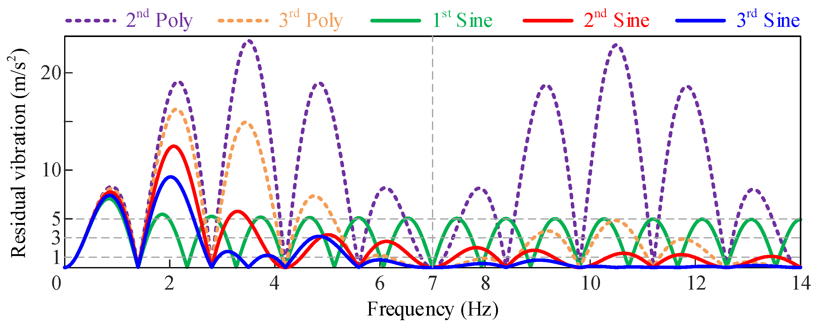
To quantitatively assess robustness, we introduce a sensitivity curve that captures the variation in the residual vibration magnitude as a function of the uncertain natural frequency. Figure 10 illustrates the residual vibration amplitude obtained for each motion profile designed by the proposed zero placement strategy when the actual natural frequency deviates from the nominal value of 7 Hz . In this plot, the residual vibration amplitude increases as the mismatch between the assumed and actual vibration characteristics becomes larger; however, the rate of increase depends strongly on the type and order of the motion profile. In general, the results show that motion profiles with higher order tend to be less sensitive to uncertainty and maintain lower residual vibration over a wider frequency range. In addition, for the same profile order, sine-based motion profiles tend to provide stronger vibration attenuation than polynomial-based profiles, indicating that the frequency-domain shaping achieved by time-shifted sine trajectories can yield more favorable robustness properties than conventional polynomial profiles. This broad frequency-domain attenuation is particularly advantageous for MDOF systems. When the profile is tuned to the fundamental mode, the residual vibration levels in the higher-frequency bands—which correspond to secondary or higher-order modes in an MDOF system—remain significantly lower for sine-based profiles compared to polynomial designs. Therefore, for applications where suppressing vibrations in the 2nd or higher-order modes is critical, selecting the proposed sine-based motion profile can be an efficient choice.
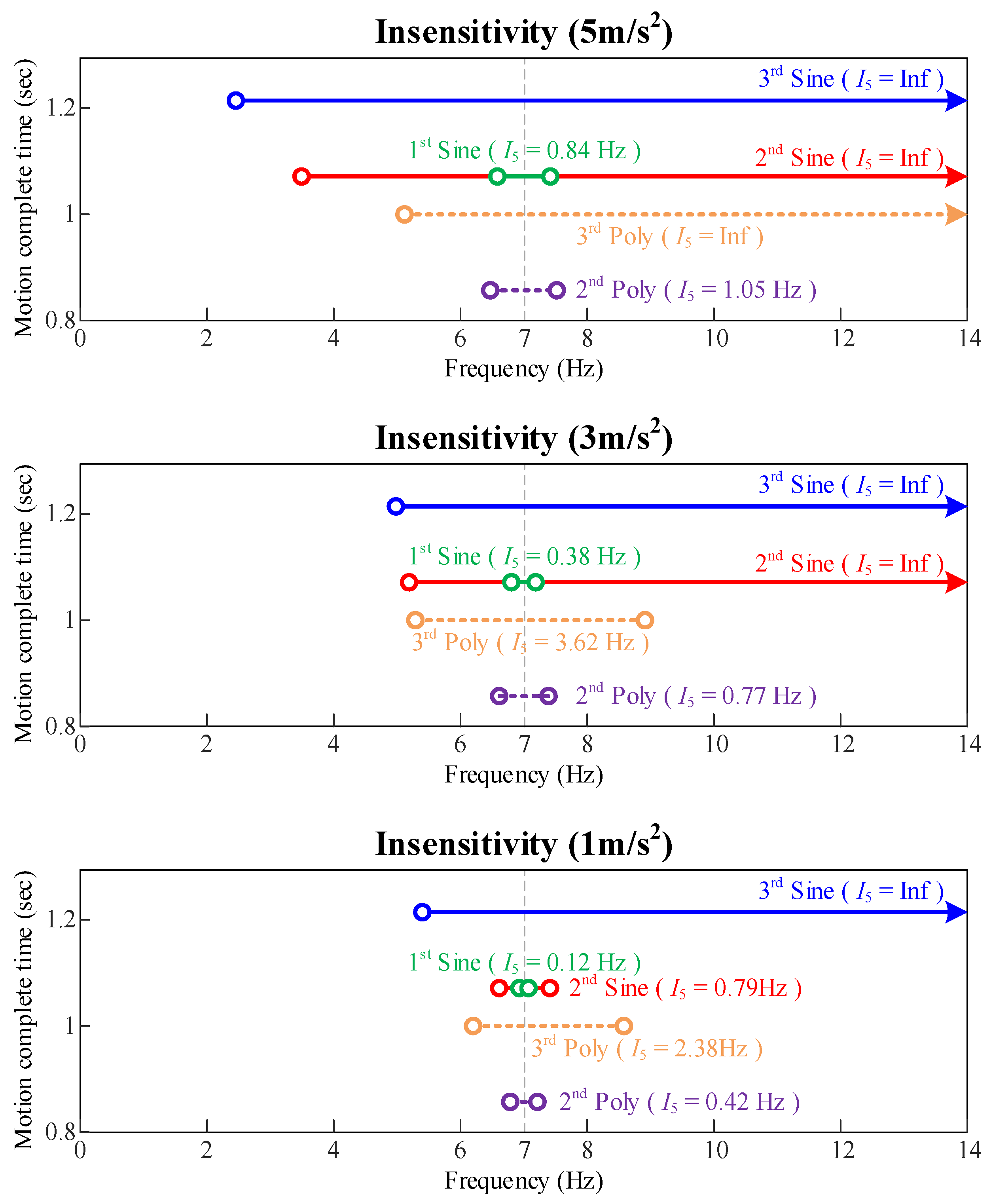
To interpret robustness more systematically, we characterize the uncertainty tolerance using the concept of insensitivity. As defined in Figure 11, insensitivity is the range of natural frequency over which the residual vibration remains below a specified bound, referred to as the insensitivity bound. In this study, several bounds are considered to represent different application requirements, including 5 m / s 2 , 3 m / s 2 , and 1 m / s 2 . A wider insensitivity range indicates that the designed motion profile can robustly suppress residual vibration even in the presence of larger modeling uncertainties. For example, in the 3rd Sine case, the insensitivity range for the bound 5 m / s 2 is [ 2.46 Hz , ) , for 3 m / s 2 is [ 4.99 Hz , ) , and for 1 m / s 2 is [ 5.40 Hz , ) . This example demonstrates that as the required residual-vibration bound becomes more stringent, the acceptable frequency-uncertainty range becomes narrower, reflecting an inevitable trade-off between robustness and vibration performance. Using the same procedure, we measured insensitivity ranges for all motion profiles and summarized the results together with motion completion times in Figure 12, providing a practical guideline for selecting motion profiles based on uncertainty levels and vibration constraints.
Based on the robustness results, the “best” motion profile selection depends on both the uncertainty range and the required vibration bound. For instance, if the residual vibration must be guaranteed within 5 m / s 2 (approximately 0.5 g) under system uncertainties of ± 20 % , corresponding to the frequency interval [ 5.6 Hz , 8.4 Hz ] , the 3rd Poly (S-curve) profile remains the most effective choice because it provides the shortest motion completion time while maintaining sufficient vibration suppression within that uncertainty range. However, if the uncertainty requirement becomes significantly stricter—for example, ensuring the same residual-vibration bound under ± 50 % uncertainty, corresponding to [ 3.5 Hz , 10.5 Hz ] —then the best choice shifts to the 2nd Sine profile, which provides a notably wider insensitivity region and thus maintains robust vibration suppression over a much broader variation in natural frequency. Furthermore, in scenarios where the allowable residual-vibration limit is more restrictive, such as requiring the residual vibration to remain within 1 m / s 2 (approximately 0.1 g) under ± 20 % uncertainty, the 3rd Sine profile becomes the most suitable option because it provides the strongest vibration attenuation capability under strict vibration constraints.
In practical engineering applications, selecting an appropriate motion profile is not simply a matter of choosing the fastest trajectory; rather, control engineers must make a decision by jointly considering multiple system requirements and constraints, including moving distance, velocity and acceleration limits, permissible residual-vibration magnitude, and the uncertainty range of the system vibration characteristics. Importantly, robustness should not be evaluated only near the nominal natural frequency. Real transfer systems often contain unmodeled dynamics and may exhibit multiple vibration modes in the higher-frequency range, meaning that vibration suppression at frequencies beyond the nominal mode can also be critical. For this reason, it is desirable to evaluate not only the sensitivity around the nominal frequency but also the attenuation characteristics over a broader frequency spectrum.
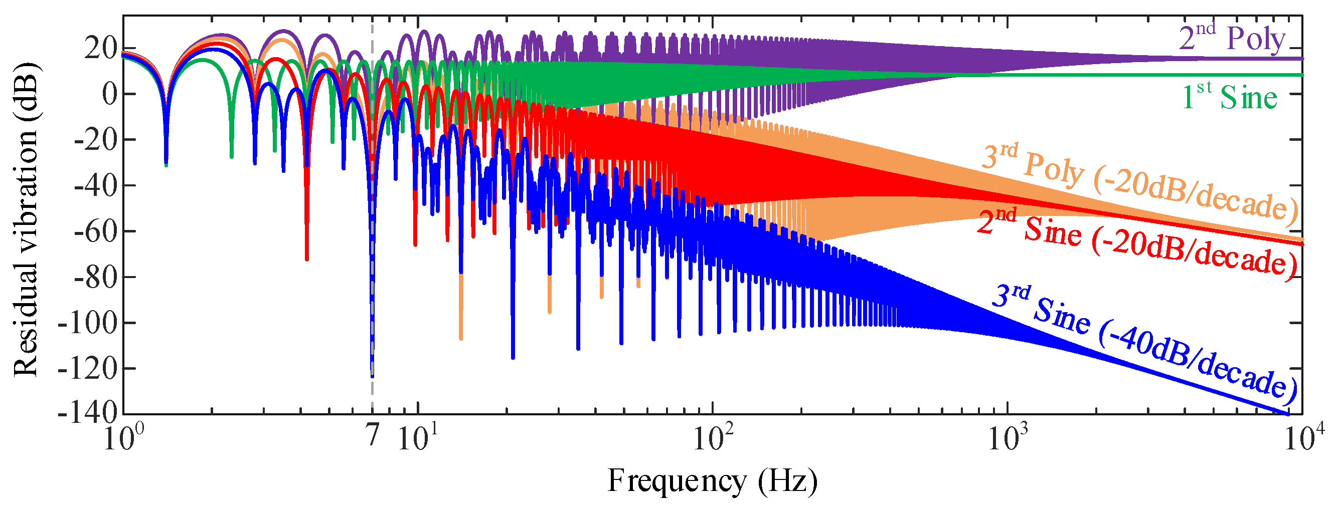
To this end, Figure 13 presents the same residual-vibration variation data as Figure 10 but visualized over a broader frequency range with a logarithmic x-axis and a decibel (dB) scale on the y-axis. This representation allows the robustness trend in the high-frequency region to be more clearly interpreted. In particular, the high-frequency robustness can be characterized by the concept of roll-off, defined as the slope of the sensitivity curve in the high-frequency region when plotted in decibels over a logarithmic frequency axis. The results show that as the order of the motion profile increases, the roll-off becomes steeper, indicating improved attenuation of vibration sensitivity in the high-frequency range. More specifically, increasing the motion-profile order by one typically improves the roll-off by approximately 20 dB / decade . For example, the roll-off of the 2nd Sine profile is approximately 20 dB / decade steeper than that of the 1st Sine profile, and the 3rd Sine profile further improves the roll-off by another 20 dB / decade compared to the 2nd Sine profile. This trend can be interpreted from the perspective of motion smoothness: higher-order motion profiles generate smoother trajectories, which reduce abrupt changes in the motion command and consequently decrease the energy injected into high-frequency components. In addition, for the same order, sine-based motion profiles exhibit approximately 20 dB / decade steeper roll-off than polynomial-based profiles, implying that time-shifted sine motion profiles provide superior high-frequency robustness compared with conventional polynomial trajectories. This observation is particularly meaningful for MDOF systems where higher-frequency unmodeled modes can be excited by fast motion commands. Consequently, for precision systems where suppressing vibrations across multiple high-frequency modes is a priority, the improved high-frequency attenuation makes the proposed sine-based profiles a more efficient and reliable solution.
In summary, the proposed zero placement method enables the design of time-shifted sine family motion profiles (1st/2nd/3rd Sine) to achieve high-speed transfer with minimal vibration excitation. The simulation results further confirm that these sine-based motion profiles can robustly suppress residual vibration even in the presence of modeling errors, i.e., when the actual natural frequency deviates from the nominal value. In particular, the time-shifted sine family consistently exhibits superior uncertainty tolerance by maintaining low residual vibration over a wider range of natural-frequency variations, while also providing improved attenuation characteristics in the high-frequency region. Moreover, the insensitivity metric and roll-off analysis indicate that increasing the profile order enhances robustness and strengthens vibration suppression near the nominal mode as well as across a broader frequency range. Therefore, when robustness against system uncertainties is a key requirement, sine-based motion profiles designed via zero placement offer a practical and highly effective solution, whereas polynomial-based motion profiles primarily serve as reference baselines for comparison.

6. Case Study: Simulation for Short-Stroke Scenario

In addition to the long-stroke cases discussed above, we consider a short-stroke scenario to examine how the profile selection changes with moving distance. While the results discussed above indicate that the 1st Sine motion profile (time-shifted sine velocity profile) does not offer a clear advantage in terms of motion completion time and also exhibits inferior robustness against modeling uncertainties compared to higher-order sine profiles, this observation does not necessarily imply that the 1st Sine profile is always an unfavorable choice. In particular, when the required moving distance is very short, lower-order motion profiles can become not only feasible but also highly advantageous. To this end, we consider a short-stroke operating scenario and show that the performance trade-offs observed in long-stroke motions do not directly translate to short-stroke cases.
A key difference between polynomial-based and sine-based motion profiles lies in the minimum profile order required to satisfy physical realizability under velocity and acceleration constraints. For polynomial-based motion profiles, at least a 2nd-order profile is required to satisfy both velocity and acceleration limits, which results in a trapezoidal velocity trajectory. In contrast, sine-based motion profiles remain physically realizable even at the 1st-order. Specifically, the 1st Sine motion profile, defined by a time-shifted sine velocity function, inherently ensures continuous velocity and bounded acceleration, allowing it to be implemented without violating physical constraints. This property enables the realization of lower-order motion profiles in sine-based designs and makes the 1st Sine profile particularly attractive for applications involving short moving distances.
Short-stroke motions are not exceptional cases but occur frequently in practical operating environments. For instance, in wafer-handling robots, extremely short vertical or horizontal motions are repeatedly required during wafer pick-up and placement processes, where minimizing vibration is critical to avoid wafer damage and to ensure high throughput [28,29,30]. Similarly, in high-speed pick-and-place systems, fine adjustment motions over small strokes are often performed after coarse positioning to achieve accurate placement. Another representative example can be found in precision assembly or inspection equipment, where small corrective motions are repeatedly executed to align parts, sensors, or optical components. In these applications, the moving distance is short, and fast execution with low residual vibration is critical, while system uncertainties are not severe.
To investigate this short-stroke scenario in detail, we consider the same system parameters used in the earlier analyses—namely, a velocity limit V lim = 1 m / s , an acceleration limit A lim = 6 m / s 2 , a natural frequency f n = 7 Hz , and a damping ratio ζ = 0.001 —while reducing the moving distance to a short stroke of D = 0.05 m . Under this condition, various motion profiles were designed using the proposed zero placement approach, and the resulting motion-induced vibration of the second mass was evaluated as the base follows each designed trajectory. The corresponding motion profiles and vibration responses are shown in Figure 14, which provides a direct comparison of residual vibration levels and motion completion times in a short-stroke operating case.
As shown in Figure 14, the short-stroke case exhibits behavior that is clearly different from that observed in long moving-distance motions. Among the considered motion profiles, the 1st Sine motion profile achieves the shortest motion completion time while still maintaining a low level of residual vibration. This indicates that, for short moving distances, the performance advantage of higher-order motion profiles becomes less pronounced. As a result, despite its relatively simple structure, the 1st Sine motion profile can be an effective and practical choice for short-stroke motions when system uncertainties are not significant, offering a good balance between fast execution and residual vibration reduction.
To further clarify this observation from a robustness perspective, Figure 15 summarizes the insensitivity characteristics and motion completion times of the considered motion profiles for the short-stroke case under insensitivity bounds of 5, 3, and 1 m / s 2 . The results indicate that, although the 1st Sine motion profile exhibits a narrower insensitivity range than the higher-order profiles, it achieves the shortest motion completion time. Therefore, when system uncertainties remain moderate and rapid motion execution is critical, the 1st Sine motion profile becomes a competitive and practical option for short-stroke motions. These results further highlight that, even within the same zero placement design framework, the preferred motion profile depends strongly on the operating conditions, particularly the moving distance and the expected level of system uncertainty.
From a practical design standpoint, these findings suggest that motion-profile selection should not be based on a single performance metric or a single operating condition. Instead, control engineers should consider the combined effects of moving distance, required motion completion time, allowable residual vibration level, and the expected range of system uncertainties. For short-stroke motions with moderate uncertainty levels, prioritizing fast execution through a lower-order sine-based profile, such as the 1st Sine, can lead to superior overall performance. Conversely, as the moving distance increases or as robustness against larger modeling uncertainties becomes more critical, higher-order sine motion profiles provide more reliable vibration suppression at the expense of slightly longer motion completion times. Therefore, the proposed zero placement approach offers a practical design guideline that enables motion profiles to be systematically selected and tailored according to specific operating regimes rather than relying on a single universally optimal trajectory.

7. Conclusions

This paper presented a systematic framework for the design of optimized time-shifted sine motion profiles for high-speed positioning systems subject to vibration constraints. Unlike conventional time-domain trajectory design approaches, the proposed method integrates time-domain profile construction with Laplace-domain analysis, enabling a unified derivation from 1st-order to generalized n th -order profiles.
A key theoretical result of this study is that the residual vibration amplitude after motion completion is proportional to the magnitude of the Laplace-domain quantity | s X ( s ) | evaluated at the system poles. This finding establishes a clear analytical link between motion-profile design and vibration suppression, and it provides the theoretical foundation for the proposed closed-form zero placement strategy. Based on this insight, explicit algebraic design conditions were derived for 1st-, 2nd-, 3rd-, and generalized n th -order time-shifted sine profiles, allowing vibration-oriented parameter tuning without relying on iterative numerical optimization.
Simulation-based case studies demonstrated that, although time-optimal profiles minimize pure travel time, they may induce significant transient and residual vibrations. In contrast, the proposed zero placement approach drastically reduces residual vibration while maintaining competitive motion completion times. Quantitative comparisons showed that the proposed method achieves near-vibration-free arrival, particularly for higher-order sine profiles.
Robustness against modeling uncertainties was further analyzed using the concepts of insensitivity and high-frequency roll-off. The results revealed that increasing the motion-profile order systematically improves robustness, expanding the acceptable natural-frequency variation range and enhancing high-frequency attenuation. In particular, each increase in profile order improves the roll-off by approximately 20 dB/decade, and sine-based profiles exhibit steeper attenuation characteristics than polynomial-based counterparts of the same order.
Additionally, a short-stroke case study highlighted that lower-order sine profiles, especially the 1st-order time-shifted sine velocity profile, can become highly advantageous when the moving distance is small and uncertainty levels are moderate. This demonstrates that the optimal motion-profile selection depends strongly on operating conditions, including stroke length, allowable vibration bounds, and expected parameter uncertainty.
Overall, the proposed closed-form zero placement framework provides a practical and scalable design guideline for vibration-aware motion control. By enabling systematic trade-off management among motion speed, vibration suppression, and robustness, the method offers an effective solution for high-speed precision positioning systems operating under realistic uncertainty conditions.


Author Contributions

Conceptualization, C.-W.H.; methodology, C.-W.H.; software, C.-W.H.; validation, D.L.; formal analysis, D.L.; investigation, C.-W.H.; writing—original draft preparation, C.-W.H.; writing—review and editing, D.L.; visualization, C.-W.H. All authors have read and agreed to the published version of the manuscript.

Funding

This research was funded by the National Research Foundation of Korea (NRF) grant funded by the Korea government (MSIT) (No. RS-2026-25473823) and (No. RS-2025-02223634, ERC, Kookmin University); by the Institute of Information & Communications Technology Planning & Evaluation (IITP) grant funded by the Korea government (MSIT) (No. RS-2025-02219317, AI Star Fellowship, Kookmin University); and by the research grant of Kongju National University Industry-University Cooperation Foundation in 2025.

Institutional Review Board Statement

Not applicable.

Informed Consent Statement

Not applicable.

Data Availability Statement

No new data were created or analyzed in this study. Data sharing is not applicable to this article.

Conflicts of Interest

The authors declare no conflicts of interest. The funders had no role in the design of the study; in the collection, analyses, or interpretation of data; in the writing of the manuscript; or in the decision to publish the results.

References

  1. Harris, C.M.; Piersol, A.G. Harris’ Shock and Vibration Handbook; McGraw-Hill: New York, NY, USA, 2002; Volume 5. [Google Scholar]
  2. Biagiotti, L.; Melchiorri, C. Online planning of multi-segment trajectories with trigonometric blends. IFAC Proc. Vol. 2011, 44, 10343–10348. [Google Scholar] [CrossRef] [Scilit]
  3. Ha, C.W.; Lee, D. Analysis of embedded prefilters in motion profiles. IEEE Trans. Ind. Electron. 2017, 65, 1481–1489. [Google Scholar] [CrossRef] [Scilit]
  4. Li, H.; Le, M.; Gong, Z.; Lin, W. Motion profile design to reduce residual vibration of high-speed positioning stages. IEEE/ASME Trans. Mechatron. 2009, 14, 264–269. [Google Scholar] [CrossRef] [Scilit]
  5. Uchiyama, N.; Honda, Y.; Sano, S. Residual vibration suppression and energy saving in industrial machines using a trapezoidal velocity profile. In 2014 American Control Conference; IEEE: New York, NY, USA, 2014; pp. 323–328. [Google Scholar]
  6. Berardinis, L. Motion control gets gradually better. Mach. Des. 1994, 66, 90–93. [Google Scholar]
  7. Meckl, P.; Arestides, P. Optimized s-curve motion profiles for minimum residual vibration. In Proceedings of the 1998 American Control Conference, ACC (IEEE Cat. No.98CH36207); IEEE: New York, NY, USA, 1998; Volume 5, pp. 2627–2631. [Google Scholar] [CrossRef] [Scilit]
  8. Gasparetto, A.; Zanotto, V. A technique for time-jerk optimal planning of robot trajectories. Robot. Comput.-Integr. Manuf. 2008, 24, 415–426. [Google Scholar] [CrossRef] [Scilit]
  9. Olabi, A.; Béarée, R.; Gibaru, O.; Damak, M. Feedrate planning for machining with industrial six-axis robots. Control Eng. Pract. 2010, 18, 471–482. [Google Scholar] [CrossRef] [Scilit]
  10. Barre, P.J.; Bearee, R.; Borne, P.; Dumetz, E. Influence of a jerk controlled movement law on the vibratory behaviour of high-dynamics systems. J. Intell. Robot. Syst. 2005, 42, 275–293. [Google Scholar] [CrossRef] [Scilit]
  11. Rew, K.H.; Kim, K.S. A closed-form solution to asymmetric motion profile allowing acceleration manipulation. IEEE Trans. Ind. Electron. 2009, 57, 2499–2506. [Google Scholar] [CrossRef] [Scilit]
  12. Chen, J.H.; Yeh, S.S.; Sun, J.T. An S-curve acceleration/deceleration design for CNC machine tools using quintic feedrate function. Comput.-Aided Des. Appl. 2011, 8, 583–592. [Google Scholar] [CrossRef] [Scilit]
  13. Perumaal, S.S.; Jawahar, N. Automated trajectory planner of industrial robot for pick-and-place task. Int. J. Adv. Robot. Syst. 2013, 10, 100. [Google Scholar]
  14. Perumaal, S.; Jawahar, N. Synchronized trigonometric S-curve trajectory for jerk-bounded time-optimal pick and place operation. Int. J. Robot. Autom. 2012, 27, 385. [Google Scholar] [CrossRef] [Scilit]
  15. Lin, Z.; Li, Y.; Qian, Q.; Haung, F.; Zhang, X.; Zhang, T.; Wang, W. Construction of an improved semi-physical simulation system for UAV with integrated energy-consumption prediction model and its evaluation of the path planning algorithms in mountainous scenery. Comput. Ind. Eng. 2024, 197, 110601. [Google Scholar] [CrossRef] [Scilit]
  16. Robertson, M.J. Experimental verification of saturation reducing, zero vibration command shapers. In Proceedings of the 2009 American Control Conference; IEEE: New York, NY, USA, 2009; pp. 4939–4944. [Google Scholar]
  17. Biagiotti, L.; Melchiorri, C. FIR filters for online trajectory planning with time-and frequency-domain specifications. Control Eng. Pract. 2012, 20, 1385–1399. [Google Scholar] [CrossRef] [Scilit]
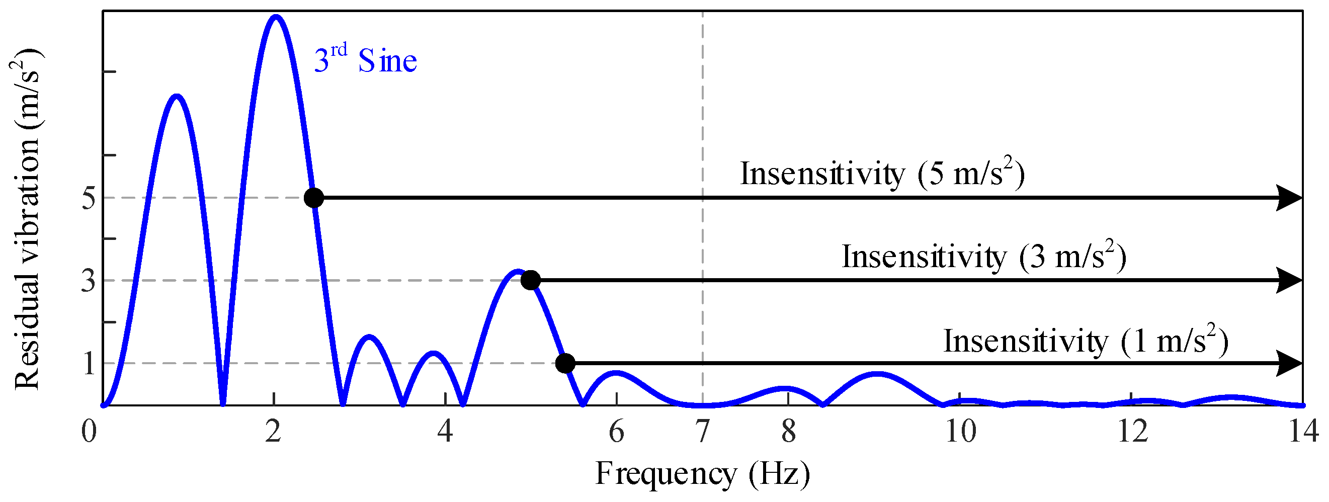
  18. Biagiotti, L.; Melchiorri, C. Trajectory generation via FIR filters: A procedure for time-optimization under kinematic and frequency constraints. Control Eng. Pract. 2019, 87, 43–58. [Google Scholar] [CrossRef] [Scilit]
  19. Biagiotti, L.; Melchiorri, C. Optimization of generalized S-curve trajectories for residual vibration suppression and compliance with kinematic bounds. IEEE/ASME Trans. Mechatron. 2020, 26, 2724–2734. [Google Scholar] [CrossRef] [Scilit]
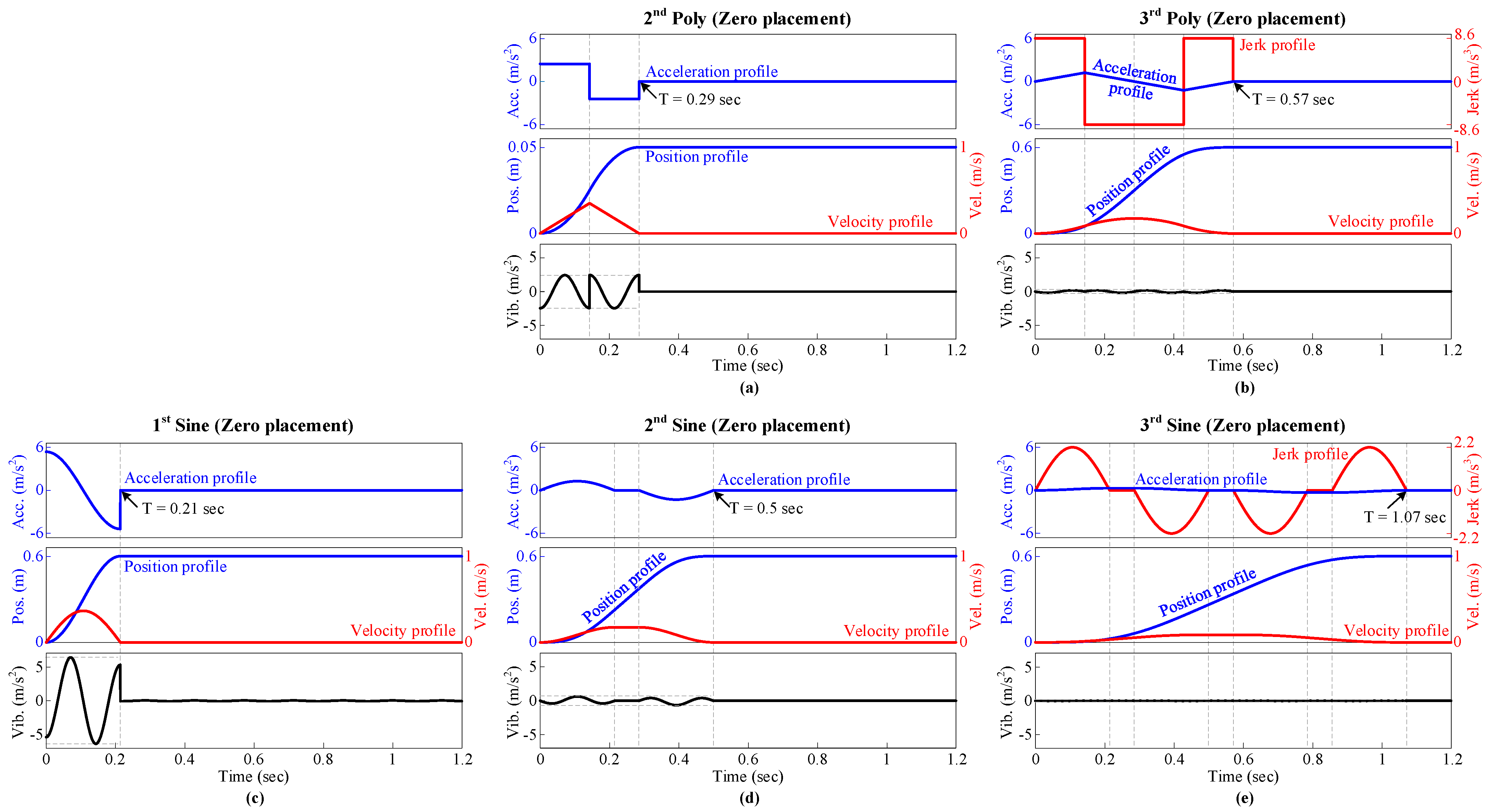
  20. Biagiotti, L.; Melchiorri, C.; Moriello, L. Optimal trajectories for vibration reduction based on exponential filters. IEEE Trans. Control Syst. Technol. 2015, 24, 609–622. [Google Scholar] [CrossRef] [Scilit]
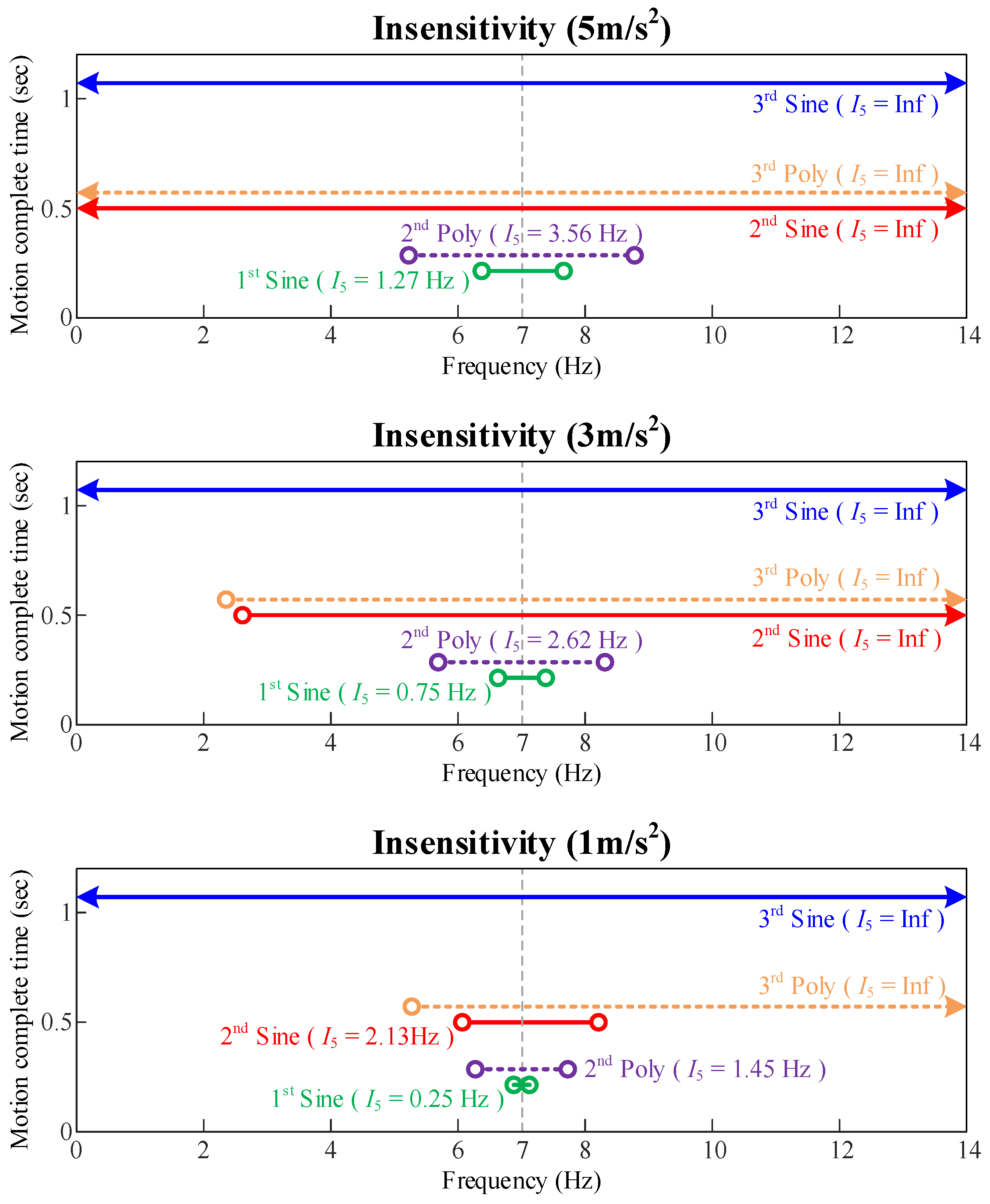
  21. Fang, Y.; Zhu, G.N.; Zhao, Y.; Gu, C. Design procedure for motion profiles with sinusoidal jerk for vibration reduction. Appl. Sci. 2023, 13, 13320. [Google Scholar] [CrossRef] [Scilit]
  22. Nguyen, K.D.; Ng, T.C.; Chen, I.M. On algorithms for planning s-curve motion profiles. Int. J. Adv. Robot. Syst. 2008, 5, 11. [Google Scholar] [CrossRef] [Scilit]
  23. Ha, C.W.; Lee, D. Optimal placement of inherent zeros in polynomial-based motion profiles for minimizing residual vibration and travel time under system uncertainties. ISA Trans. 2024, 152, 467–476. [Google Scholar] [CrossRef] [Scilit] [PubMed]
  24. Ha, C.W.; Rew, K.H.; Kim, K.S. Robust zero placement for motion control of lightly damped systems. IEEE Trans. Ind. Electron. 2012, 60, 3857–3864. [Google Scholar] [CrossRef] [Scilit]
  25. Lee, D.; Ha, C.W. Optimization process for polynomial motion profiles to achieve fast movement with low vibration. IEEE Trans. Control Syst. Technol. 2020, 28, 1892–1901. [Google Scholar] [CrossRef] [Scilit]
  26. Balula, S.; Liao-McPherson, D.; Rupenyan, A.; Lygeros, J. Data-driven reference trajectory optimization for precision motion systems. Control Eng. Pract. 2024, 144, 105834. [Google Scholar] [CrossRef] [Scilit]
  27. Qiu, Z.C.; He, C.H.; Zhang, X.M. Trajectory planning optimization and probabilistic inference reinforcement learning vibration control of three translational flexible beams. Proc. Inst. Mech. Eng. Part G J. Aerosp. Eng. 2026, 240, 209–226. [Google Scholar] [CrossRef] [Scilit]
  28. Ha, C.W. Robust Airgap Stabilization of a Magnetic Levitation Wafer Handling Robot Under Harsh Operating Conditions via Acceleration Feedforward and Disturbance Observer. Int. J. Precis. Eng. Manuf. 2025, 27, 939–954. [Google Scholar] [CrossRef] [Scilit]
  29. Ha, C.W.; Kim, C.H.; Lim, J. Development of levitation control for high accuracy magnetic levitation transport system. J. Inst. Control. Robot. Syst. 2016, 22, 557–561. [Google Scholar] [CrossRef] [Scilit]
  30. Yoon, K.S.; Kim, M.S.; Moon, H.; Choi, H.R.; Koo, J.C. An Asymmetric Velocity Profile for Minimizing Wafer Slippage and Settling Time of a Wafer Transport Robot. Electronics 2023, 12, 2157. [Google Scholar] [CrossRef] [Scilit]
Figure 1. Time-domain shapes of the basis functions used for motion profile generation: (a) sine-function-based basis function and (b) rectangular pulse basis function.
Applsci 16 03098 g001
Figure 2. Time-shifted sine position profile illustrating physical unrealizability due to infinite acceleration at the motion onset.
Applsci 16 03098 g002
Figure 3. Time-shifted sine velocity profile.
Applsci 16 03098 g003
Figure 4. Time-shifted sine acceleration profile.
Applsci 16 03098 g004
Figure 5. Time-shifted sine jerk profile.
Applsci 16 03098 g005
Figure 6. Transfer system with a flexible structure.
Applsci 16 03098 g006
Figure 7. Pole-zero cancellation when (a) τ 1 = 0.5 T d and (b) τ 1 = 1.5 T d for the 1st-order time-shifted sine motion profile.
Applsci 16 03098 g007
Figure 8. Time-shifted sine velocity/acceleration/jerk profile tuned via time-optimal (ac) and proposed zero placement (df) approaches, together with the corresponding motion-induced vibration.
Applsci 16 03098 g008
Figure 9. Motion profiles designed using the proposed zero placement approach and the resulting motion-induced vibrations under modeling uncertainties, where the actual natural frequency varies by 0%, 5%, 10%, 15%, 20%, 25%, and 30% relative to the nominal one.
Applsci 16 03098 g009
Figure 10. Variation of the residual vibration amplitude under system uncertainties for different motion profiles designed using the proposed zero placement approach: trapezoidal velocity profile (2nd Poly), S-curve (3rd Poly), time-shifted sine velocity profile (1st Sine), time-shifted sine acceleration profile (2nd Sine), and time-shifted sine jerk profile (3rd Sine).
Applsci 16 03098 g010
Figure 11. Definition of insensitivity as the range of natural frequency over which the residual vibration remains below a specified bound.
Applsci 16 03098 g011
Figure 12. Insensitivity and motion completion time for various motion profiles designed using the proposed zero placement approach under different insensitivity bounds ( 5 m / s 2 , 3 m / s 2 , and 1 m / s 2 ).
Applsci 16 03098 g012
Figure 13. Variation of the residual vibration amplitude under system uncertainties, shown on a logarithmic x-axis and expressed in decibels on the y-axis.
Applsci 16 03098 g013
Figure 14. Motion profiles designed using the proposed zero placement approach and the resulting motion-induced vibration for a short-stroke case (D = 0.05 m ).
Applsci 16 03098 g014
Figure 15. Insensitivity and motion completion time for various motion profiles designed via the zero placement approach in a short-stroke case ( D = 0.05 m ) under insensitivity bounds of 5, 3, and 1 m / s 2 .
Applsci 16 03098 g015
Table 1. Simulation Parameters for physical constraints and system vibration characteristics.
CategoryParameterNotationValue
Physical constraintsMoving distanceD ( m )0.6 (Long-stroke)
0.05 (Short-stroke)
Velocity limit V lim ( m / s )1
Acceleration limit A lim ( m / s 2 )6
System vibration characteristicsNatural frequency f n ( Hz )7
Damping ratio ζ (-)0.001
Table 2. Comparison of motion-profile parameters for time-optimal and zero placement designs.
1 st Sine 2 nd Sine 3 rd Sine
Time-OptimalZero PlacementTime-OptimalZero PlacementTime-OptimalZero Placement
T ( s )0.941.070.861.070.841.21
τ 1 ( s )0.94 (6.6 T d )1.07 (7.5 T d )0.26 (1.8 T d )0.36 (2.5 T d )0.07 (0.5 T d )0.21 (1.5 T d )
τ 2 ( s )0.60 (4.2 T d )0.71 (5 T d )0.17 (1.2 T d )0.29 (2 T d )
τ 3 ( s )0.60 (4.2 T d )0.71 (5 T d )
V max ( m / s )1.000.881.000.841.000.84
A max ( m / s 2 )3.332.586.003.706.002.94
J ( m / s 3 )13222
y ¨ t r , p p ( m / s 2 )6.695.177.741.7916.060.57
y ¨ r e s , p p ( m / s 2 )3.950.247.03 7.4 × 10 4 10.86 1.3 × 10 6
Disclaimer/Publisher’s Note: The statements, opinions and data contained in all publications are solely those of the individual author(s) and contributor(s) and not of MDPI and/or the editor(s). MDPI and/or the editor(s) disclaim responsibility for any injury to people or property resulting from any ideas, methods, instructions or products referred to in the content.