Hybrid Attribution-Based Interpretable Deep Reinforcement Learning for Autonomous Driving Behavior Decision-Making

Abstract

With the increasing deployment of autonomous driving systems, the opaque nature of deep reinforcement learning (DRL) decision models hinders understanding and validation of driving decisions. To address this challenge, we propose a Hybrid Attribution-based Interpretable Deep Reinforcement Learning framework (HA-IDRL) for autonomous driving behavior decision-making. The framework introduces a Hybrid Gradient–LRP (HGL) attribution mechanism that integrates gradient-based attribution and Layer-wise Relevance Propagation (LRP) to capture complementary sensitivity and contribution information, producing more consistent and comprehensive post hoc explanations. In addition to post hoc interpretability, we enhance structural interpretability by replacing the conventional multilayer perceptron (MLP) in the Dueling Deep Q-Network (Dueling DQN) architecture with Kolmogorov–Arnold Networks (KAN). By representing nonlinear interactions through learnable univariate functions and explicit summation structures, KAN provides inherently interpretable functional decompositions. The proposed framework is evaluated on a highway lane-changing task using the highway-env simulator. Experimental results show that HA-IDRL achieves decision-making performance comparable to representative DRL baselines, including Dueling DQN and Soft Actor-Critic (SAC), while providing explanations that are more stable and better aligned with human driving semantics. Moreover, the proposed method produces explanations with low computational overhead, enabling efficient and real-time interpretability in practical autonomous driving applications. Overall, HA-IDRL advances trustworthy autonomous driving by enabling high-performance decision-making and rigorous, multi-level interpretability, thereby improving the transparency and operational reliability of DRL-based driving policies.

1. Introduction

Autonomous driving systems typically consist of multiple functional modules, including environment perception, behavior decision-making, motion planning, and vehicle control. Among them, behavior decision-making and motion planning play a critical role in complex traffic environments, where vehicles must simultaneously consider safety, traffic efficiency, driving comfort, and interactions with surrounding traffic participants to generate high-level driving decisions or trajectories [1,2].

Early approaches to autonomous driving behavior decision-making and planning relied mainly on rule-based or model-driven methods, such as finite-state machine-based lane-changing logic [3], cost-function-based search planning [4], and traffic-flow-driven models, including the well-known MOBIL lane-changing model [5]. These methods exhibit clear structural interpretability and perform reliably in controlled or low-complexity scenarios. Nevertheless, their firm reliance on handcrafted rules results in high design costs and limited scalability, making it difficult to generalize to complex, highly interactive traffic environments.

To overcome these limitations, data-driven learning-based approaches have been increasingly adopted. Supervised learning and imitation learning methods have been widely applied to learn driving behaviors from human expert demonstrations, significantly reducing the burden of manual rule design [6,7]. However, such methods are sensitive to the distribution of the training data. When encountering unseen scenarios, behavioral variations of other traffic participants, or perception-induced distribution shifts, their performance often degrades substantially [8]. Moreover, the lack of closed-loop interaction with the environment limits their ability to optimize long-term decision objectives.

In recent years, reinforcement learning (RL) has emerged as a promising paradigm for autonomous driving decision-making. By continuously interacting with the environment and optimizing policies based on reward feedback, RL enables agents to learn decision strategies that maximize long-term returns directly. In particular, the development of deep reinforcement learning (DRL) introduces deep neural networks to approximate high-dimensional state–action mappings, allowing end-to-end policy learning in complex state spaces. Representative DRL algorithms include value-based methods such as Deep Q-Network (DQN) [9] and its variants (e.g., Double Deep Q-Network (DDQN) [10], Dueling Deep Q-Network (Dueling DQN) [11]), as well as policy-based and actor–critic approaches such as Proximal Policy Optimization (PPO) [12] and Soft Actor-Critic (SAC) [13]. Compared with supervised or imitation learning, DRL alleviates performance degradation under distribution shifts to some extent and demonstrates strong adaptability and flexibility in tasks such as highway driving, lane-changing, and multi-vehicle coordination [14].

In parallel with the rapid development of deep reinforcement learning, extensive research has focused on improving neural network architectures and training strategies to enhance learning efficiency and model generalization. For instance, neural architecture search (NAS) has been widely studied to automatically discover efficient network structures and improve model design efficiency, significantly reducing the need for manual architecture engineering [15]. Graph neural networks (GNNs) have been applied to represent traffic scenes as structured graphs, where detected objects are modeled as nodes and their relationships are constructed through interaction patterns among traffic participants [16]. Recently, state-space-based architectures such as Mamba have been proposed for efficient long-sequence modeling with linear computational complexity, providing a promising alternative to transformer-based models [17]. Meanwhile, reinforcement learning algorithms have also evolved rapidly. Distributional reinforcement learning improves value estimation by modeling the full return distribution rather than its expectation [18], while recent studies on representation learning for reinforcement learning aim to learn informative state–action representations to improve policy learning efficiency and generalization in complex environments [19]. However, despite these advances, most existing studies primarily focus on improving model performance and representation capability, while paying limited attention to the interpretability of the learned decision policies. Artificial neural networks (ANNs), particularly multilayer perceptrons (MLPs), have long been criticized for their lack of interpretability, which limits their practical deployment in safety-critical systems [20]. In such domains, providing reliable explanations is essential for increasing user trust and system acceptance [21], simplifying model verification and validation [22], facilitating error diagnosis and correction [23], and supporting compliance with regulatory requirements and standards [24,25].

Despite these advantages, DRL significantly exacerbates the interpretability challenge. The highly nonlinear and hierarchically coupled structure of deep neural networks makes the internal decision-making process difficult to understand [26]. Interpretability is a critical prerequisite for safety evaluation, decision validation, and trustworthiness of autonomous driving systems. The lack of transparent explanations can substantially increase uncertainty and potential risks in complex or extreme traffic situations [27,28].

To improve the interpretability of DRL-based decision-making models, existing studies have explored various approaches, which can be broadly categorized into three classes. The first class adopts intrinsically interpretable structures, such as decision trees [29], finite-state machines [30], or prototype-based learning [31], in which the decision logic is inherently interpretable. However, their limited expressive capacity often restricts their applicability to complex dynamic traffic scenarios. The second class focuses on post hoc explanation methods that infer decision rationales by analyzing input–output relationships without modifying the original network structure. Representative methods include LIME [32] and SHAP [33]. While these methods are model-agnostic, their explanations are often decoupled from the internal representations of DRL models, limiting their fidelity to the actual decision process. The third class attempts to directly explain the internal mechanisms of neural networks, such as Integrated Gradients [34] and Layer-wise Relevance Propagation (LRP) [35], which quantify feature-level contributions to the decision output. Although these methods provide fine-grained explanations, their robustness and stability are often compromised by the deep nonlinear coupling inherent in conventional MLP architectures.

In our previous work [36], we have explored combining Kolmogorov–Arnold Networks (KAN) [37] with LRP to enhance structural interpretability by leveraging explicit nonlinear function representations. By replacing scalar weights with learnable univariate functions, KAN provides clearer semantic pathways for attribution propagation. Experimental results in [36] further indicate that attribution methods applied to KAN-based models can produce clearer and more stable explanations compared with those obtained from conventional MLP architectures. However, LRP primarily focuses on contribution allocation and is relatively insensitive to feature perturbations, particularly near decision boundaries. In contrast, gradient-based methods effectively capture local sensitivity but tend to underestimate feature importance in saturated regions where gradients vanish.

Motivated by this complementary behavior, this paper proposes a Hybrid Gradient–LRP (HGL) attribution method that integrates sensitivity-based and contribution-based explanations within a unified framework. Building upon this attribution mechanism, we further develop a Hybrid Attribution-based Interpretable Deep Reinforcement Learning framework (HA-IDRL) for autonomous driving behavior decision-making. The proposed approach simultaneously enhances structural interpretability through KAN-based value function modeling and feature-level interpretability through hybrid attribution, enabling more comprehensive, stable, and semantically aligned explanations without sacrificing decision performance.

The main contributions of this work are summarized as follows:

• We extend gradient-based sensitivity analysis to the KAN-based value function and integrate it with LRP-based contribution allocation, thereby proposing a hybrid attribution mechanism. The proposed method provides computationally efficient, real-time, comprehensive, and semantically aligned explanations for DRL decision-making.
• We introduce KAN into the Dueling DQN framework to enhance structural interpretability and improve the consistency of attribution propagation.
• We validate the proposed HA-IDRL framework on a highway lane-changing task, demonstrating that it achieves competitive driving performance while significantly improving interpretability quality.

The rest of this paper is structured as follows:

Section 2 introduces the proposed interpretable decision-making framework and its theoretical motivation. Section 3 presents the simulation experiments, including the experimental configuration, evaluation metrics, and performance evaluation results. Section 4 further analyzes the interpretability of the proposed framework through local, counterfactual, and global attribution analyses. Finally, Section 5 concludes the paper.

2. Interpretable Deep Reinforcement Learning Methodology

Due to the highly nonlinear mapping from state observations to action selection, the internal decision logic of DRL policies remains largely opaque, making it difficult to analyze, validate, and trust autonomous driving behaviors.

To address this limitation, this section establishes the theoretical foundation for the proposed HA-IDRL framework, designed to improve the interpretability of DRL-based decision-making in autonomous driving. The HA-IDRL framework provides a unified perspective for interpreting DRL-based driving decisions from multiple complementary viewpoints.

Within this framework, structural interpretability is achieved by KAN into the decision model; sensitivity-based interpretability is captured through gradient attribution; and contribution-based interpretability is modeled via LRP, together with the proposed hybrid attribution strategy. The following subsections present the theoretical foundations of these components and their integration within the overall HA-IDRL framework.

2.1. HA-IDRL Framework Overview

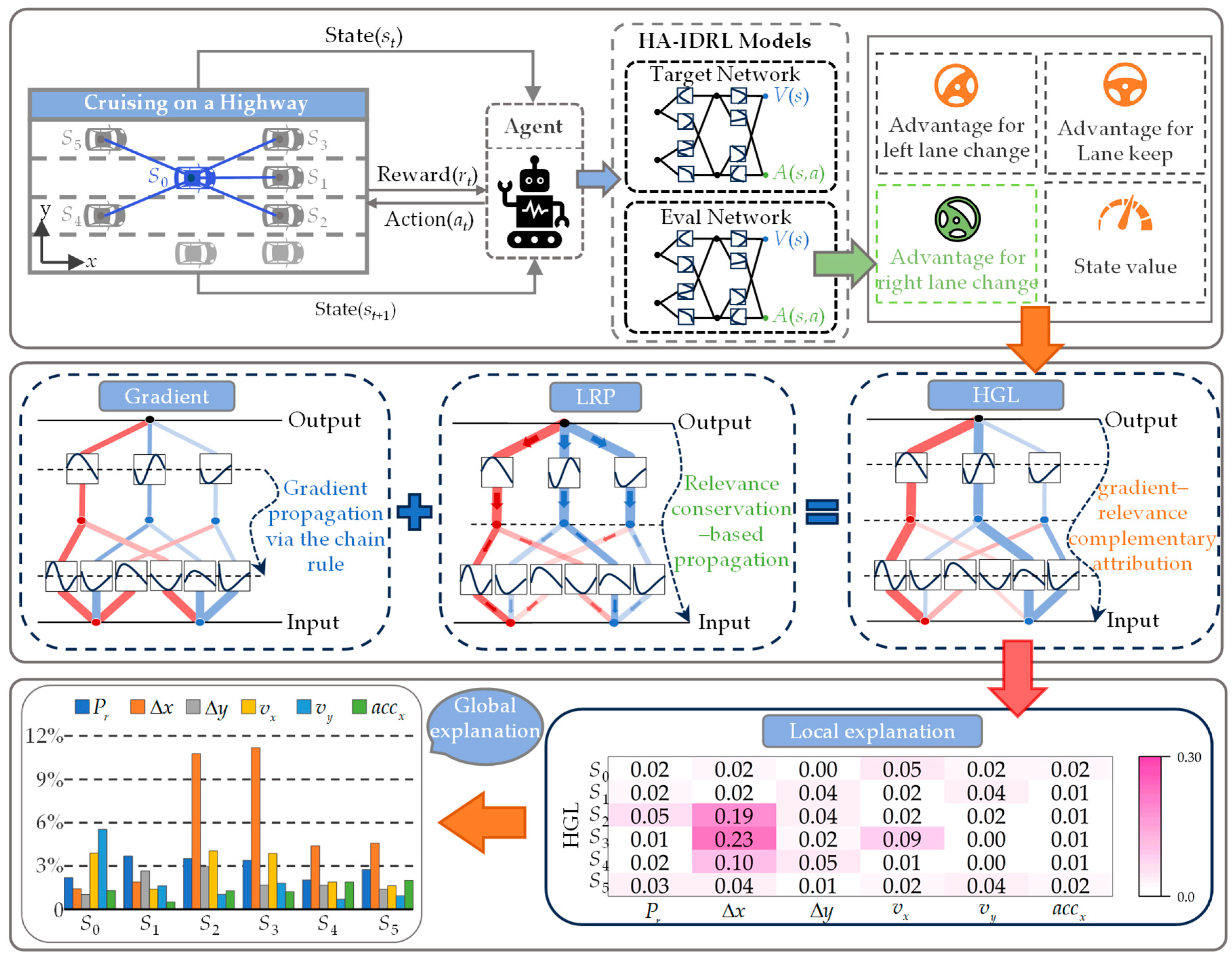
We propose an HA-IDRL framework for autonomous driving decision-making, as illustrated in Figure 1. The proposed approach falls within the emerging field of interpretable reinforcement learning, which aims to improve the transparency of reinforcement learning policies while maintaining strong decision performance. The HA-IDRL framework represents a practical implementation of this paradigm.

The framework adopts a Dueling DQN-based decision model as its core, preserving original decision performance while introducing multi-level interpretability mechanisms. Given a state s, the policy network outputs action-value estimates and selects the optimal action. In parallel, the interpretability module analyses the decision rationale at both structural and feature levels.

At the structural level, KAN replace conventional MLP to provide explicit nonlinear functional representations that enable attribution signals to propagate along well-defined, interpretable functional pathways. At the feature level, gradient attribution captures local sensitivity, while LRP quantifies global contribution. These complementary signals are fused through HGL to generate comprehensive, stable, and semantically aligned explanations.

By jointly integrating structural, feature-level, and decision-level interpretability, HA-IDRL forms a unified explanatory loop that enables transparent, verifiable, and semantically meaningful analysis of autonomous driving decisions.

2.2. Kolmogorov–Arnold Networks for Value Function Modeling

Conventional DRL methods typically employ an MLP to approximate value functions. Nonlinearity is introduced through fixed activation functions such as ReLU or Tanh. Although effective in practice, this modeling paradigm relies on deeply coupled parameters, resulting in opaque internal representations and limited structural interpretability.

Several interpretable structures have been explored to improve the transparency of decision-making systems, including decision trees, prototype-based models, and finite-state machines (FSMs). Decision trees provide rule-based explanations but often suffer from scalability issues when handling high-dimensional state spaces and continuous control tasks commonly encountered in autonomous driving. Prototype-based models interpret predictions by comparing inputs with representative examples; however, maintaining meaningful prototypes becomes challenging when the state distribution evolves during reinforcement learning. Finite-state machines offer explicit state-transition logic but lack the flexibility required to model complex nonlinear interactions in dynamic traffic environments. Consequently, directly integrating these structures into modern deep reinforcement learning frameworks is difficult, as they often sacrifice either modeling capability or training efficiency.

To address this limitation, we adopt KAN as the function approximator within the DRL framework. KAN are theoretically grounded in the Kolmogorov–Arnold representation theorem, which states that any continuous multivariate function f(x) can be decomposed into a finite sum of univariate functions, as shown in Equation (1).

$$f(x)={\displaystyle \sum _{k=1}^K{\varphi }_k\left({\displaystyle \sum _{i=1}^d{\varphi }_{k,i}(x_i)}\right)}$$

(1)

where ${\varphi }_k(\cdot )$ and ${\varphi }_{k,i}(\cdot )$ are continuous univariate functions.

Inspired by this theorem, KAN explicitly introduces nonlinear modeling capability into network connections by replacing scalar weights with learnable univariate functions. In practice, these functions are parameterized using continuous and differentiable multi-grid B-spline bases, enabling flexible yet structured nonlinear approximation. The fundamental computation of a KAN layer is defined in Equation (2).

$$y_j ={\displaystyle \sum _{i=1}^d{\varphi }_{ij}} \left(x_i\right)$$

(2)

where ${\varphi }_{ij}(\cdot )$ denotes the learnable univariate function mapping input $x_i$ to output node j. For the l-th layer, the input feature vector is defined as Equation (3).

$$h^{(l)}=\left[h_1^{(l)},h_2^{(l)},\dots ,h_n^{(l)}\right]$$

(3)

Then the output of the layer is computed according to Equation (4).

$$h_j^{\left(l+1\right)}={\displaystyle \sum _{i=1}^{d_l}{\varphi }_{ij}^{(l)}}\left(h_i^{\left(l\right)}\right)$$

(4)

where ${\varphi }_{ij}^{(l)}$ represents the learnable univariate function between nodes i and j at layer l.

Through this layered composition, KAN represents high-dimensional nonlinear mappings as structured combinations of learnable univariate functions. As discussed in the original KAN work [37], such a representation provides a more transparent functional structure compared with conventional MLP, since each connection is modeled as an explicit univariate function rather than a scalar weight. This structural formulation preserves expressive capability while maintaining explicit relationships between input variables and output responses. The same study also reports that KAN can achieve comparable representation capability with significantly smaller network structures and fewer layers, which facilitates attribution-based analysis. Moreover, recent studies have shown that attribution methods applied to KAN-based models can produce clearer and more stable explanations compared with those applied to conventional MLP architectures [36]. These properties provide a structural basis for gradient-based and relevance-based attribution analysis.

In this work, we integrate KAN into the Dueling DQN architecture by replacing the MLP-based value networks with KAN. Specifically, KAN are used to parameterize both the state-value function V(s) and the action-advantage function A(s, a), while preserving the original value–advantage decomposition and optimization objectives. This modification introduces structural interpretability into the decision-making model without altering the underlying reinforcement learning algorithm.

2.3. Gradient-Based Attribution with KAN

The theoretical formulation of combining KAN with LRP-based relevance propagation has been established in [25], and is therefore not elaborated in detail in this work.

Gradient-based attribution is a widely used interpretability technique that quantifies the relative importance of input features by analyzing how the model’s output changes with input perturbations. Formally, the gradient of the model output provides a first-order local approximation of how changes in each input dimension influence the decision.

When combined with KAN, gradient attribution exhibits enhanced structural clarity. From Equation (2), the partial derivative of the output with respect to an input dimension can be expressed as Equation (5).

$${\displaystyle \frac{\partial y_j}{\partial x_i}} ={\displaystyle \sum _{i=1}^n{\varphi }_{ij}^{\prime }\left(x_i\right)}$$

(5)

This formulation indicates that the gradient depends solely on the derivative of the corresponding univariate function, rather than on entangled multi-dimensional interactions.

From the layer-wise formulation in Equation (4), the Jacobian element of the $l$-th layer can be expressed as Equation (6).

$$J^{\left(l\right)}\triangleq {\displaystyle \frac{\partial h_j^{\left(l+1\right)}}{\partial h_j^{\left(l\right)}}}={\left[{\left({\varphi }_{ij}^{(l)}\right)}^{\prime }\left(h_i^{\left(l\right)}\right)\right]}_{j,i}$$

(6)

Let the KAN-based value network be a scalar-output function $f(x)$. The end-to-end gradient with respect to the input is computed via the chain rule, as shown in Equation (7).

$$\nabla x f(x)={\left(J^{(0)}\right)}^{\top }{\left(J^{(1)}\right)}^{\top }\dots {\left(J^{(n)}\right)}^{\top }$$

(7)

and the gradient attribution for the k-th input dimension is defined as Equation (8).

$${\displaystyle \frac{\partial f(x)}{\partial s_k}}={\displaystyle \sum _{\left(i_1,\dots ,i_L\right)}{\displaystyle \prod _{l=0}^L{\left({\varphi }_{i_l i_{l+1}}^{(l)}\right)}^{\prime }}}\left(h_{i_l}^{\left(l\right)}\right)$$

(8)

where gradients accumulate along all valid functional paths in the network.

Compared with conventional MLP, attribution propagation in KAN follows semantically explicit functional pathways, which effectively mitigate entanglement in propagation paths caused by deep nonlinear coupling. This property facilitates clearer interpretation for both gradient-based and relevance-based attribution methods, as illustrated by the structural comparison between MLP and KAN in

Table 1. Comparison of interpretation methods based on different networks. $h_i^{\left(l\right)}$ denotes the hidden representation of neuron i at layer l; w_ij represents the connection weight between neurons $i$ and $j$; $\sigma (\cdot )$ denotes the activation function in MLP; ${\varphi }_{ ij}(\cdot )$ denotes the learnable univariate function used in KAN; and $R_i^{\left(l\right)}$ represents the relevance score propagated in LRP.

Model	MLP	KAN
Recurrence Formula	$h_j^{\left(l+1\right)}=\sigma ({\displaystyle \sum _j{w}_{ij}{h}_i^{\left(l\right)}+w_k})$	$h_j^{\left(l+1\right)}={\varphi }_{ ij}(h_i^{\left(l\right)})$
Gradient Attribution	${\displaystyle \frac{\partial h_j^{\left(l+1\right)}}{\partial h_i^{\left(l\right)}}}=\sigma \prime \left(h_j^{(l+1)}\right)\hspace{0.33em}{w}_{ij}$	${\displaystyle \frac{\partial h_j^{\left(l+1\right)}}{\partial h_i^{\left(l\right)}}}=\left({\varphi }_{ ij}^{\left(l\right)}\right)\prime \left(h_i^{(l)}\right)$
LRP	$R_i^{(l)}={\displaystyle \sum _j\frac{h_i^{\left(l\right)}{w}_{ij}}{{\displaystyle {\sum }_{0,i}{h}_i^{\left(l\right)}{w}_{ij}}}{R}_j^{(l+1)}}$	$R_i^{(l)}={\displaystyle \sum _j\frac{{\varphi }_{ ij}\left(h_i^{\left(l\right)}\right)}{{\displaystyle {\sum }_{0,i}{\varphi }_{ ij}\left(h_i^{\left(l\right)}\right)}}{R}_j^{(l+1)}}$
Multi Layer Framework

.

For reinforcement learning, gradient attribution is applied to the action-value function, using a first-order Taylor expansion around state s, as shown in Equation (9).

$$Q(s+\mathrm{\Delta }s,a)\approx Q(s,a)+\nabla s Q{(s,a)}^{\top }\mathrm{\Delta }s$$

(9)

where the gradient vector is defined as Equation (10).

$$\nabla sQ(s,a)={\left[{\displaystyle \frac{\partial Q(s,a)}{\partial s_1}} ,\dots ,{\displaystyle \frac{\partial Q(s,a)}{\partial s_n}}\right]}^{\top }$$

(10)

Thus, the gradient vector $\nabla sQ(s,a)$ can be interpreted as a feature-level sensitivity measure. Under the Dueling DQN decomposition, the action-value function is defined as Equation (11).

$$Q(s,a)=V(s)+A(s,a)$$

(11)

Based on Equation (11), the gradient naturally decomposes as Equation (12).

$$\nabla sQ(s,a)=\nabla sV(s)+\nabla sA(s,a)$$

(12)

Accordingly, gradient attribution can be separately defined for the state-value branch and the action-advantage branch, as shown in Equations (13) and (14), respectively.

$$g_V=\nabla sV(s)$$

(13)

$$g_A=\nabla sA(s,a)$$

(14)

This structural decomposition aligns gradient attribution with the internal computation graph of the decision model, enabling branch-level interpretability analysis consistent with the value–advantage architecture. The overall architecture of the KAN-based reinforcement learning decision-making model for highway lane changing is illustrated in Figure 1.

2.4. Hybrid Gradient–LRP Attribution Method

Gradient attribution can provide an effective explanation of how small perturbations in state features influence action preferences near decision boundaries. However, relying solely on gradient-based attribution remains insufficient. When a feature’s influence enters a saturation regime, the model output becomes insensitive to further changes in that feature, leading to significantly reduced gradient magnitudes—even though the feature may still play a critical role in the current decision. In such cases, gradient attribution tends to underestimate the importance of saturated yet decisive features. To complement this limitation, LRP is employed to capture cumulative feature contributions in saturation regimes.

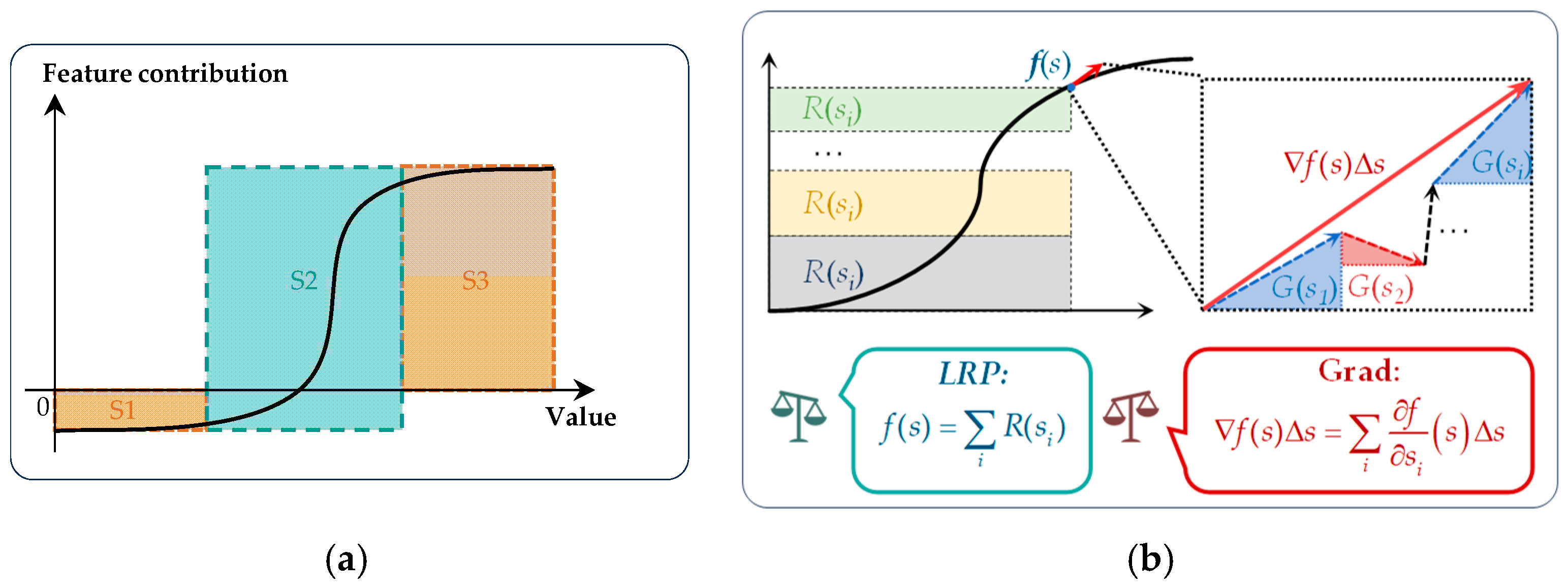
To illustrate the complementary behaviors of gradient-based attribution and LRP, Figure 2a presents a schematic relationship between a continuous state feature (e.g., the longitudinal distance to the right-front vehicle) and the decision output (e.g., lane change right).

When the feature value lies in the intermediate region (S2), the output is highly sensitive to feature variations, and gradient magnitudes are correspondingly large, effectively capturing the feature’s immediate influence on decision changes. In this region, LRP assigns relatively smaller relevance values. In contrast, when the feature enters the positive or negative saturation regions (S1 and S3), the output response becomes flat and gradient information diminishes or even vanishes, whereas LRP has large relevance scores by capturing the feature’s cumulative contribution to the current decision.

From an attribution mechanism perspective, this limitation is further clarified in Figure 2b, which compares gradient-based attribution and LRP for the same decision target $f(s)$. Gradient attribution, derived from a first-order Taylor approximation, $\nabla f(s)\mathrm{\Delta }s$ characterizes local sensitivity by approximating the output variation induced by infinitesimal input perturbations. LRP, by contrast, follows the principle of relevance conservation and redistributes the decision output backward through the network, assigning feature-level relevance scores $R(s_i)$ that reflect cumulative contribution to the current decision.

This complementary behavior motivates the proposed HGL method. Conceptually, gradient attribution captures local sensitivity, while LRP characterizes global contribution under saturation. HGL integrates these two perspectives to achieve more complete and robust explanations.

Given a decision target y (e.g., $V(s)$ or $A(s,a)$), gradient and LRP attribution vectors are computed as Equation (15).

$$g=[g_1,\dots ,g_D],\hspace{1em}r=[r_1,\dots ,r_D]$$

(15)

where D denotes the state dimension. Both vectors are normalized using an ${\mathcal{l}}_1$-norm, as shown in Equation (16).

$$\tilde{g}={\displaystyle \frac{g}{\left|\right|g|{|}_1+\epsilon }},\hspace{1em}\tilde{r}={\displaystyle \frac{r}{\left|\right|r|{|}_1+\epsilon }}$$

(16)

where $\epsilon$ is a numerical stabilization constant.

A feature-level intensity score is then defined as Equation (17).

$$a_i=\left|{\tilde{g}}_i\right|+\left|{\tilde{r}}_i\right|$$

(17)

which jointly reflects sensitivity and contribution magnitude. To suppress unstable explanations on low-intensity features, an adaptive confidence threshold is introduced, as shown in Equation (18).

$$a_i\ge \lambda \cdot \mathrm{median}(a)$$

(18)

where $\lambda$ is a scaling coefficient. Features below this threshold are excluded from explanation.

For retained features, a fusion weight is defined as Equation (19).

$$w_i={\displaystyle \frac{\left|{\tilde{g}}_i\right|}{\left|{\tilde{g}}_i\right|+\left|{\tilde{r}}_i\right|}}$$

(19)

The final hybrid attribution is then computed according to Equation (20).

$${\mathrm{I}}_i=w_i\cdot \left|{\tilde{g}}_i\right|+\left(1-w_i\right)\cdot \left|{\tilde{r}}_i\right|$$

(20)

This formulation enables HGL to adaptively emphasize gradient attribution in sensitivity-dominant regions and LRP attribution in saturation-dominant regions, thereby mitigating the limitations of either method alone. The training and explanation procedure of the proposed HA-IDRL framework is summarized in Algorithm 1.

Algorithm 1 Training and Explanation Procedure of HA-IDRL

Require: Environment Env, replay buffer M, maximum episodes T, mini-batch size N, discount factor γ Ensure: Trained KAN-based Dueling DQN model Q(s, a) and hybrid attribution result HGL 1:      Initialize environment Env, KAN-based Dueling DQN evaluation network Qθ(s, a), target network Qϕ(s, a), and replay buffer M 2:      for episode = 1 to T do 3:            Reset Env and observe initial state s0 4:            while episode not terminated do 5:                  Select action at using ε-greedy policy based on Qθ(st, a) 6:                  Execute action at in Env and observe reward rt, next state st+1, terminal flag dt 7:                  Store transition (st, at, rt, st+1, dt) in M 8:                  if M is ready for training then 9:                       Sample a mini-batch {(si, ai, ri, si+1, di)} from M 10:                     Compute target value: yi = ri + γ(1 − di) maxa′Qϕ(si+1, a′) and TD loss: L = (1/N) Σi (Qθ(si, ai) − yi)2 11:                     Update θ by minimizing L 12:                end if 13:                st ← st+1 14:                Periodically update target network ϕ ← θ 15:          end while 16:    end for 17:    Given a trained KAN-based Dueling DQN model and an input state s 18:    Compute gradient attribution g for the explained action 19:    Compute LRP attribution r for the same decision target 20:    Fuse g and r using the HGL rule to obtain I 21:    Output I as the final feature-level explanation

3. Experimental Evaluation

3.1. Simulation Environment

All experiments are conducted using the highway-env simulation platform [38], which provides a Markov Decision Process (MDP)-based formulation for modeling multi-vehicle interactions in highway driving scenarios. The environment supports longitudinal driving, lane-changing maneuvers, and multi-agent interactions, and has been widely adopted for evaluating reinforcement learning-based autonomous driving algorithms.

In this work, we construct a multi-lane highway scenario in which the ego vehicle is controlled by a reinforcement learning agent. In contrast, surrounding vehicles follow rule-based driving models to emulate realistic traffic flow. This setting enables systematic evaluation of decision-making performance in dynamic traffic interactions while maintaining a controlled, reproducible experimental setup.

In contrast to studies that rely on pre-collected driving datasets, the training data in this work are generated online through continuous interactions between the reinforcement learning agent and the simulation environment within highway-env platform [38]. At each time step, the agent observes the environment state s_t, executes an action a_t, and receives the corresponding reward r_t, next state s_t+1, and a terminal indicator d_t, forming transition tuples (s_t, a_t, r_t, s_t+1, d_t). These interaction samples are stored in a replay buffer and randomly sampled for network training. Therefore, no external dataset is required, and all training samples are produced dynamically during the simulation process.

All experiments were conducted on a workstation equipped with an Intel i9-10900K CPU (Intel Corporation, Santa Clara, CA, USA), an NVIDIA GeForce RTX 3090 GPU (NVIDIA Corporation, Santa Clara, CA, USA), and 32 GB of RAM. The proposed framework was implemented in Python 3.9.7 using the PyTorch 2.7.1 deep learning library. The simulation environment was built on the highway-env 1.10.1 platform based on the OpenAI Gym 0.26.2 interface. This hardware and software configuration provides sufficient computational resources for training and evaluating the proposed HA-IDRL framework.

3.2. State and Action Spaces

The state representation includes the ego vehicle and its nearest surrounding vehicles in adjacent lanes. Specifically, six vehicles are considered: the ego vehicle and five neighboring vehicles. A six-dimensional state vector describes each vehicle, as defined in Equation (21).

$$S_i=(P_r^{\left(i\right)},\mathrm{\Delta }{x}_i,\mathrm{\Delta }{y}_i,v_x^{\left(i\right)},v_y^{\left(i\right)},ac{c}^{\left(i\right)})$$

(21)

where $P_r^{\left(i\right)}\in \left\{0,1\right\}$ is a presence indicator specifying whether vehicle i is within the perception range (with $P_r^{\left(0\right)}=1$ for the ego vehicle), $\mathrm{\Delta }{x}_i$ and $\mathrm{\Delta }{y}_i$ denotes the longitudinal and lateral relative distances to the ego vehicle ($\mathrm{\Delta }{x}_0,\mathrm{\Delta }{y}_0$ indicates the lateral distance from the vehicle to the boundary between the right and left lanes), $v_x^{\left(i\right)},v_y^{\left(i\right)}$ represents longitudinal and lateral velocities, and $ac{c}^{\left(i\right)}$ is the longitudinal acceleration.

The overall system state is formed by concatenating the state vectors of all vehicles, resulting in a 36-dimensional state space.

A discrete action space is adopted, as defined in Equation (22).

$$\mathcal{A}=\left\{\mathit{lane} \mathit{change} \mathit{left}, \mathit{lane} \mathit{change} \mathit{right}, \mathit{keep} \mathit{lane}\right\}$$

(22)

At each time step, the agent selects an action from $\mathcal{A}$ based on the current state observation. In highway driving, the longitudinal motion of all vehicles is governed by the Intelligent Driver Model (IDM) [24], while the lane-changing decisions of surrounding vehicles are determined by the MOBIL model [5].

3.3. Reward Design

To encourage safe, efficient, and comfortable driving behaviors, the instantaneous reward at time step tis defined as a weighted sum of multiple objectives, as formulated in Equation (23).

$$r_t={\alpha }_1{r}_t^{speed}-{\alpha }_2{C}_t^{safety}-{\alpha }_3{C}_t^{fuel}-{\alpha }_4{C}_t^{comfort}$$

(23)

where ${\alpha }_1,{\alpha }_2,{\alpha }_3,{\alpha }_4>0$ are weighting coefficients controlling the relative importance of speed, safety, energy consumption, and comfort, respectively.

3.3.1. Speed Reward

To promote efficient driving, a speed reward is defined as Equation (24).

$$r_t^{speed}={\displaystyle \frac{v_t-v_{\min }}{v_{\max }-v_{\min }}},\hspace{1em}{r}_t^{speed}\in \left[0,1\right]$$

(24)

where $v_t$ is the ego vehicle’s longitudinal speed at time t, and $v_{\min }, v_{\max }$ denotes the minimum and maximum allowable speeds.

3.3.2. Safety Penalty

Safety is enforced through a penalty term that strongly discourages collisions and dangerous proximity, as defined in Equation (25).

$$C_t^{safety}=\left\{\begin{array}{l}10,\hspace{1em}\hspace{1em}\hspace{1em}\hspace{1em}\hspace{1em}if\hspace{0.33em}collision\\ 1,\hspace{1em}\hspace{1em}\hspace{1em}\hspace{1em} if\hspace{0.33em}0<d_{\min }<5\hspace{0.33em}\mathrm{m}\\ 1-{\displaystyle \frac{d_{\min }-5}{5}},\hspace{0.33em} if\hspace{0.33em}5\hspace{0.33em}\mathrm{m}\le d_{\min }<10\hspace{0.33em}\mathrm{m}\\ 0,\hspace{1em}\hspace{1em}\hspace{1em}\hspace{1em}\hspace{1em}\hspace{0.33em}otherwise\end{array}\right.$$

(25)

where $d_{\min }$ denote the distance to the closest vehicle in the same lane.

3.3.3. Energy Consumption Penalty

To approximate energy efficiency, the energy cost is modeled as a quadratic function of longitudinal acceleration, as defined in Equation (26).

$$C_t^{fuel}=ac{c}^2$$

(26)

where $acc$ is the ego vehicle’s longitudinal acceleration. This term discourages aggressive acceleration and deceleration behaviors.

3.3.4. Comfort Penalty

Driving comfort is jointly constrained by acceleration magnitude and lane-changing frequency, as defined in Equation (27).

$$C_t^{comfort}=\left|acc\right|+{\alpha }_5{\delta }_{lc}$$

(27)

where ${\alpha }_5$ is a lane-change penalty coefficient and ${\delta }_{lc}$ is an indicator function that equals 1 when a lane change action is executed, and 0 otherwise.

3.4. Baselines and Training Configuration

To evaluate the effectiveness of the proposed HA-IDRL framework, several representative reinforcement learning algorithms are selected as baselines:

• PPO: PPO is an on-policy actor–critic algorithm that stabilizes training via a clipped objective.
• SAC: SAC is an off-policy maximum entropy method that balances exploration and exploitation.
• DDQN: DDQN mitigates Q-value overestimation through decoupled action selection and evaluation.
• Dueling DQN: Dueling DQN improves learning efficiency by decomposing Q-values into state value and action advantage components.

These baselines cover both value-based and policy-gradient-based reinforcement learning paradigms. All methods are trained in the same environment and with the same reward structure to ensure a fair comparison. Hyperparameters related to optimization and environment configuration are kept consistent across algorithms unless otherwise specified. The key hyperparameters used in the experiments are summarized in

Table 2. Hyperparameters used in the experiments.

Parameter	Value
Discount Factor	0.8
Learning Rate	0.0003
Batch Size	256
MLP Hidden Units	256
Soft Update Rate	0.005
Training Update Capacity	0.005
Replay Buffer Capacity	106
Grid size (number of knots)	5
Spline Order	3
KAN Layer Width	11

.

To ensure a comprehensive evaluation across different traffic conditions, three traffic-density scenarios are considered. In the low-density scenario, the initial inter-vehicle spacing is set to 60 m, corresponding to approximately 67 vehicles per kilometer. In the medium-density scenario, the spacing is reduced to 30 m, resulting in approximately 134 vehicles per kilometer. Finally, in the high-density scenario, the spacing is further reduced to 15 m, corresponding to approximately 267 vehicles per kilometer. These density settings are selected in accordance with prior lane-changing studies [39]. The proposed models are trained and evaluated across all three traffic-density conditions.

For the low- and medium-density scenarios, training consists of 300 episodes, with each episode lasting up to 200 time steps. Each time step corresponds to one second of real-world driving time, resulting in a maximum episode duration of 200 s. For the high-density scenario, the number of training episodes is increased to 400 to account for the increased complexity of traffic interactions.

3.5. Decision-Making Performance Evaluation

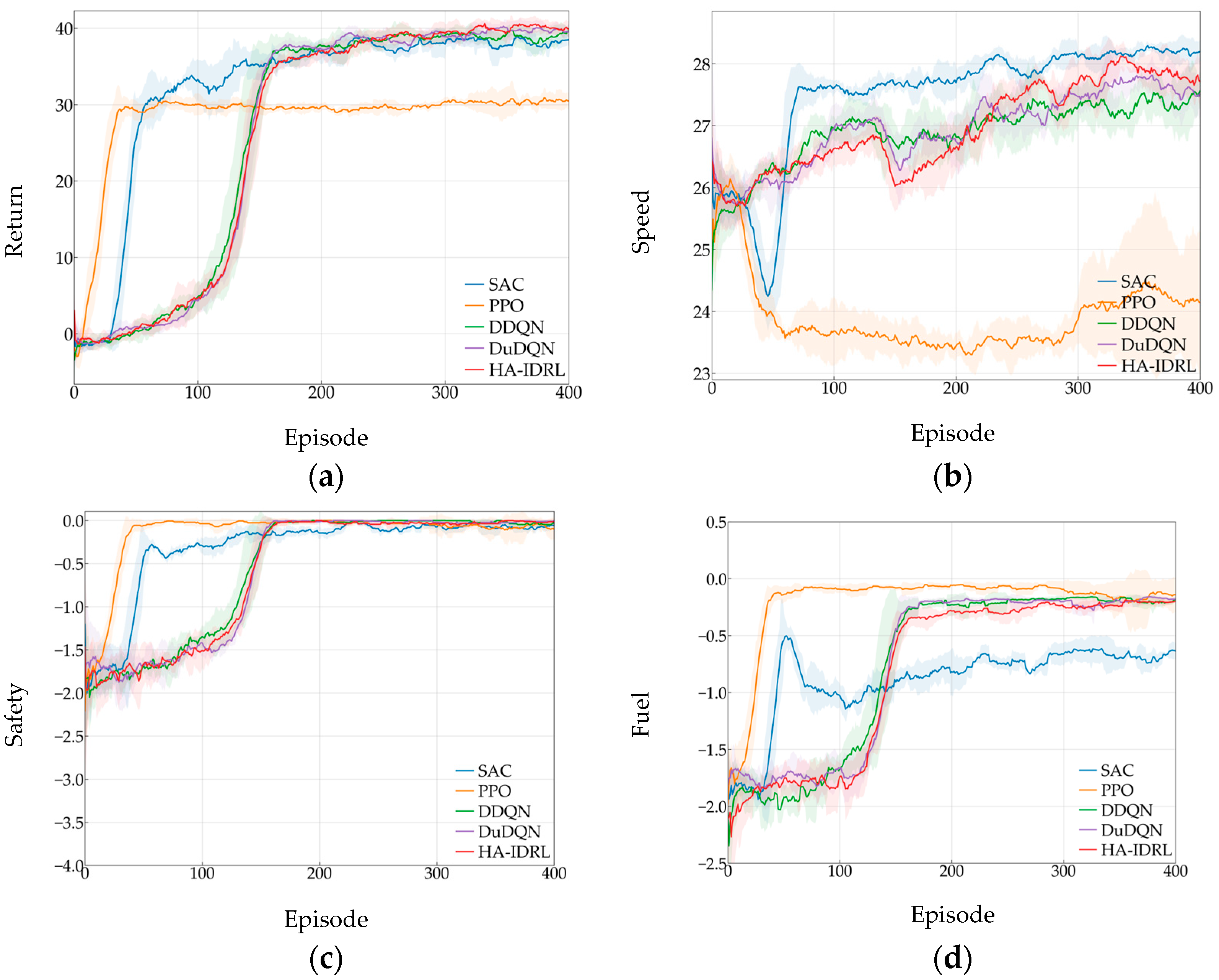
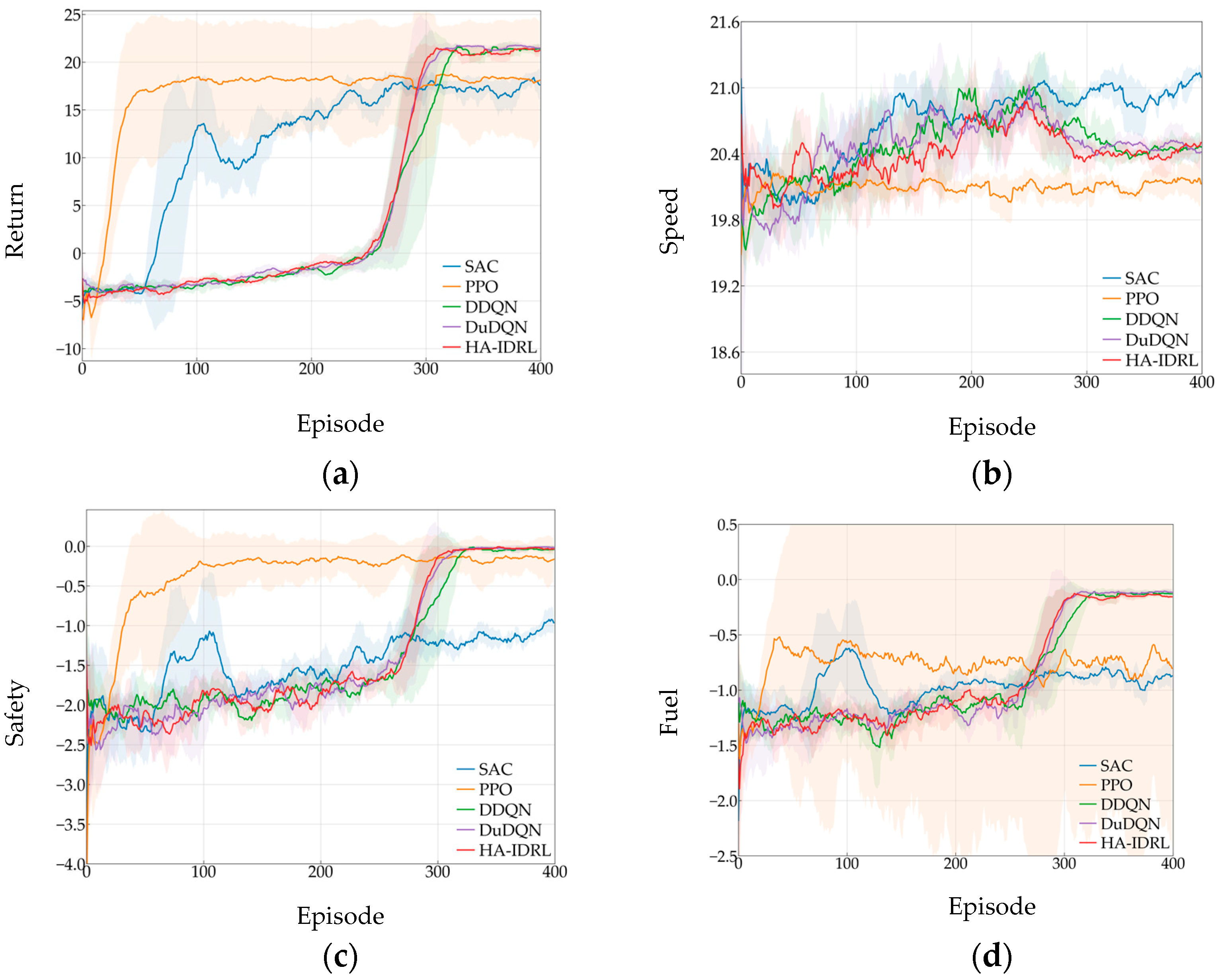
Figure 3a illustrates the evolution of average episodic return during training. Policy-gradient-based methods (e.g., PPO and SAC) achieve higher returns in the early stages of training because their on-policy update mechanisms enable rapid policy adaptation. In contrast, value-based methods require sufficient exploration to stabilize state–action value estimation, resulting in slower initial convergence but steady performance improvement.

Compared with standard Dueling DQN, the proposed HA-IDRL exhibits comparable convergence behavior and reward levels, with smooth training curves and similar variances. Figure 3b–d further report the evolution of average speed, safety penalty, and energy consumption. SAC achieves higher average speeds in later stages but incurs greater safety penalties. PPO demonstrates conservative behavior with strong early safety performance but limited speed improvement. Value-based methods maintain balanced safety and efficiency profiles throughout training.

All algorithm agents are evaluated using the same random seed, and each agent is tested over 500 evaluation episodes.

Table 3. Evaluation Results under High-Density Traffic Conditions.

Parameter	Return	Success Rate	Avg Speed	Safety	Comfort	Fuel
PPO	20.88 ± 0.09	0.95 ± 0.01	20.08 ± 0.03	−0.05 ± 0.03	−0.06 ± 0.004	−0.07 ± 0.007
SAC	19.21 ± 0.02	0.94 ± 0.02	21.13 ± 0.08	−0.71 ± 0.09	−2.44 ± 0.07	−0.75 ± 0.04
DDQN	21.49 ± 1.08	0.993 ± 0.006	20.62 ± 0.08	−0.04 ± 0.04	−0.40 ± 0.10	−0.13 ± 0.07
Dueling DQN	21.51 ± 0.12	0.991 ± 0.005	20.42 ± 0.03	−0.03 ± 0.01	−0.30 ± 0.02	−0.12 ± 0.01
HA-IDRL (Ours)	21.98 ± 0.20	0.993 ± 0.005	20.44 ± 0.015	−0.015 ± 0.01	−0.28 ± 0.02	−0.17 ± 0.018

reports the average performance of different algorithms under high-density traffic conditions. Under the high-density traffic setting, HA-IDRL achieves the highest return (21.98), the highest success rate (0.993), and the lowest absolute safety penalty (−0.015). In addition, HA-IDRL performs competitively in average speed, comfort, and fuel consumption. Compared with Dueling DQN, HA-IDRL demonstrates comparable performance across all evaluation metrics, indicating that the introduction of KAN enhances interpretability without degrading decision-making performance.

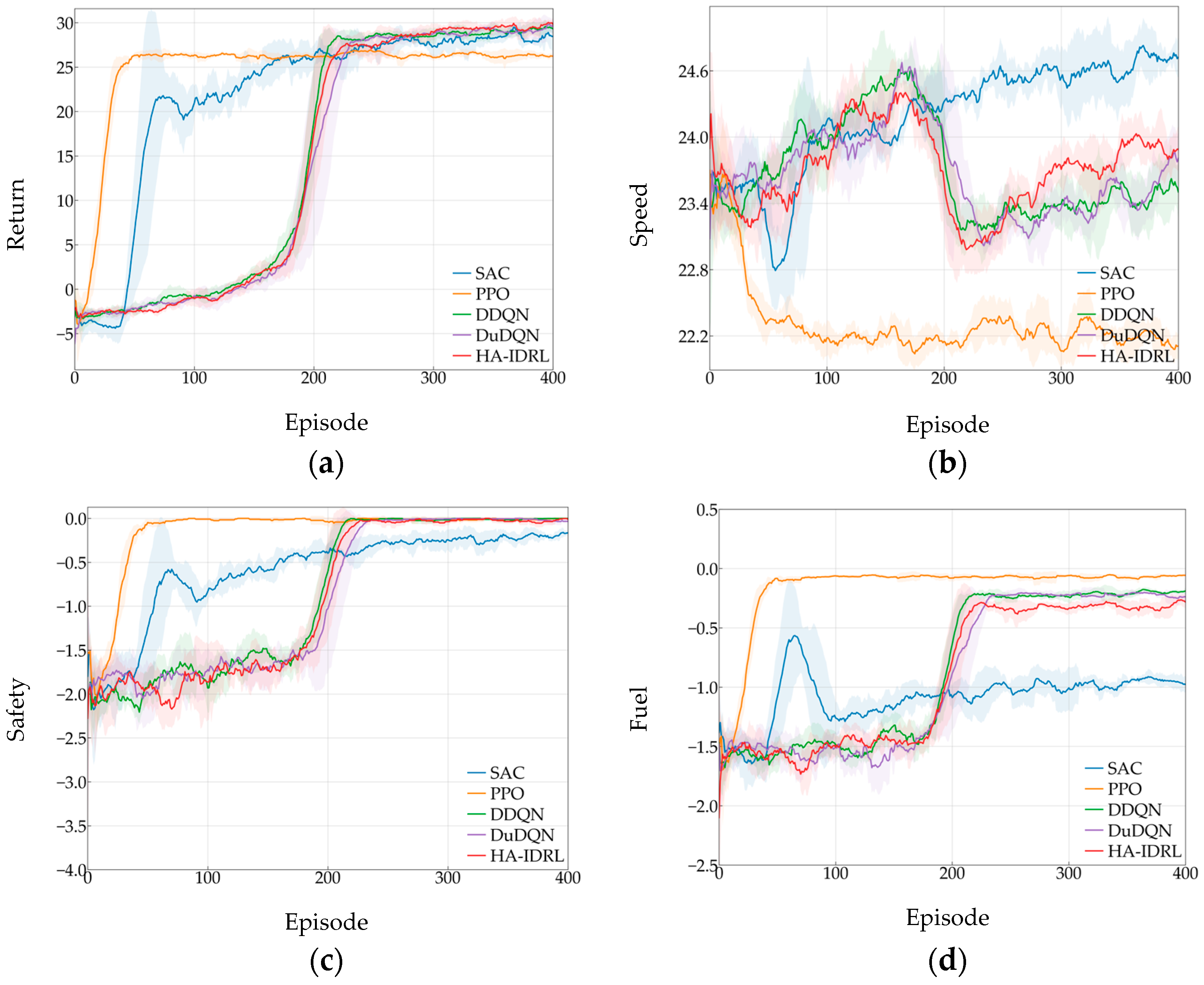
Under medium-density traffic conditions in Figure 4, the evaluation results exhibit trends similar to those observed in low-density scenarios. Value-based methods generally achieve higher returns and average speeds, indicating their effectiveness in balancing efficiency and safety under moderate traffic complexity. Notably, SAC also converges to a relatively high return and achieves the highest average speed among the methods compared. However, this increased speed is accompanied by substantially higher energy consumption, reflecting a more aggressive driving strategy. In contrast, PPO maintains a conservative behavior profile, characterized by a lower average speed and a lower return.

During the evaluation stage under low-density traffic conditions (

Table 4. Evaluation Results under Low-Density Traffic Conditions.

Parameter	Return	Success Rate	Avg Speed	Safety	Comfort	Fuel
PPO	29.80 ± 0.66	0.990 ± 0.01	23.82 ± 0.07	−0.03 ± 0.03	−0.13 ± 0.01	−0.10 ± 0.04
SAC	37.99 ± 1.02	0.95 ± 0.03	28.26 ± 0.06	−0.07 ± 0.04	−2.58 ± 0.07	−0.69 ± 0.04
DDQN	37.22 ± 0.32	0.993 ± 0.01	26.49 ± 0.15	−0.002 ± 0.004	−0.40 ± 0.01	−0.15 ± 0.01
Dueling DQN	40.42 ± 0.27	0.98 ± 0.02	28.08 ± 0.15	−0.02 ± 0.01	−0.55 ± 0.02	−0.17 ± 0.02
HA-IDRL (Ours)	40.93 ± 0.59	0.995 ± 0.01	27.79 ± 0.09	−0.001 ± 0.002	−0.59 ± 0.03	−0.18 ± 0.01

), HA-IDRL maintains strong decision-making performance and achieves the best results among the compared methods in terms of return (40.93), success rate (0.995), and safety penalty (−0.001).

As shown in Figure 5 and

Table 5. Evaluation Results under Medium-Density Traffic Conditions.

Parameter	Return	Success Rate	Avg Speed	Safety	Comfort	Fuel
PPO	26.14 ± 0.20	0.98 ± 0.01	22.16 ± 0.05	−0.02 ± 0.01	−0.08 ± 0.003	−0.07 ± 0.01
SAC	28.50 ± 0.20	0.95 ± 0.03	24.73 ± 0.06	−0.22 ± 0.02	−2.55 ± 0.02	−0.92 ± 0.02
DDQN	28.36 ± 0.49	0.98 ± 0.02	23.04 ± 0.21	−0.02 ± 0.03	−0.03 ± 0.06	−0.14 ± 0.02
Dueling DQN	29.15 ± 0.08	0.990 ± 0.01	23.77 ± 0.07	−0.01 ± 0.01	−0.56 ± 0.02	−0.23 ± 0.01
HA-IDRL (Ours)	29.69 ± 0.30	0.992 ± 0.01	23.55 ± 0.06	−0.02 ± 0.01	−0.49 ± 0.02	−0.22 ± 0.01

, under medium-density traffic conditions, the proposed HA-IDRL achieves the highest return (29.69) and success rate (0.992) among the compared methods. Meanwhile, it maintains competitive safety and efficiency performance, demonstrating a strong decision-making capability in this traffic setting.

Overall, across low-, medium-, and high-density traffic conditions, the proposed HA-IDRL framework consistently demonstrates strong and competitive decision-making performance. It achieves high return and success rates while maintaining balanced safety and efficiency metrics. These results indicate that enhancing interpretability through the proposed structural and hybrid attribution mechanisms does not compromise driving performance but instead preserves robust, reliable decision-making under varying traffic conditions.

4. Interpretability Analysis

4.1. Local Explanation Analysis

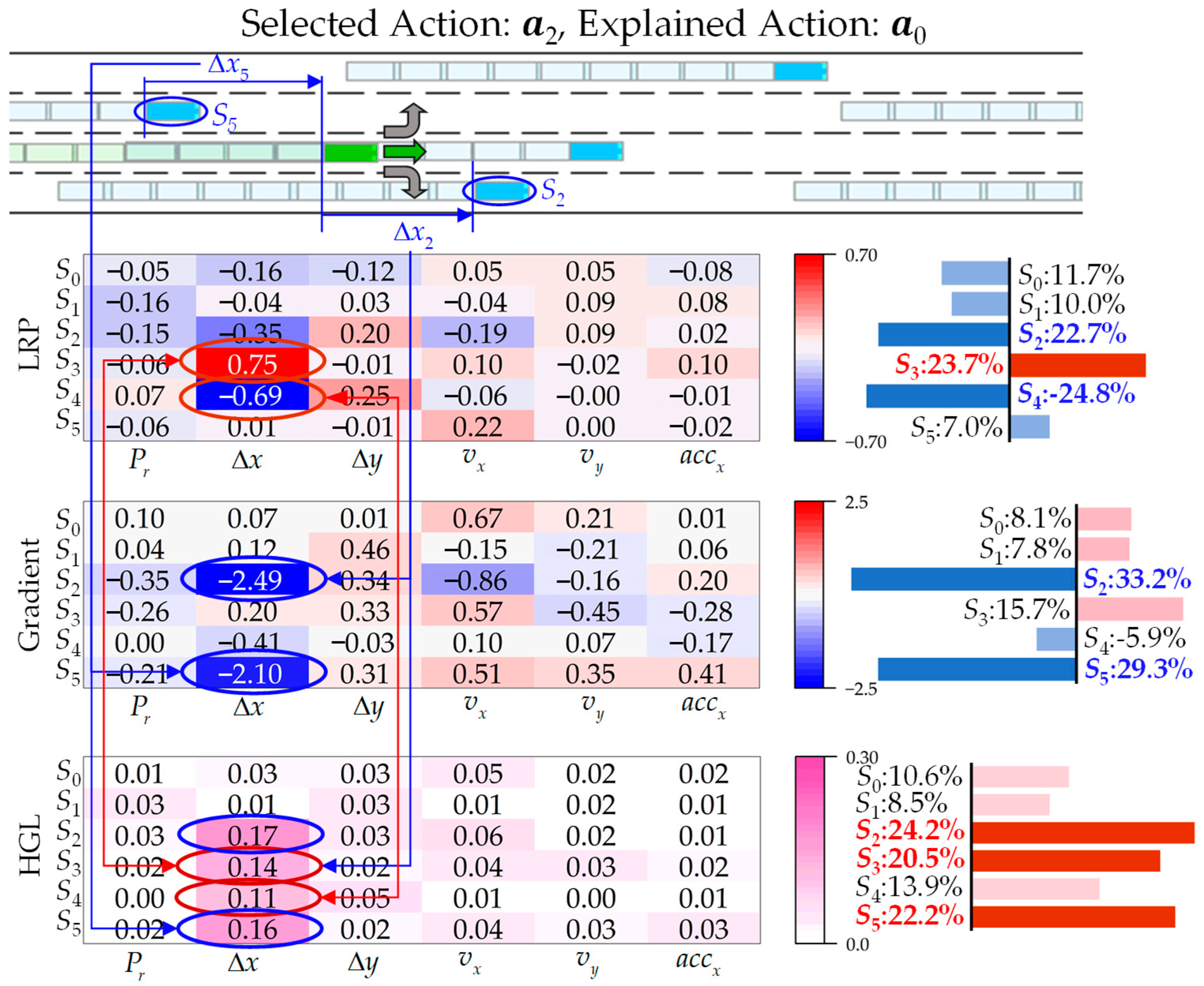
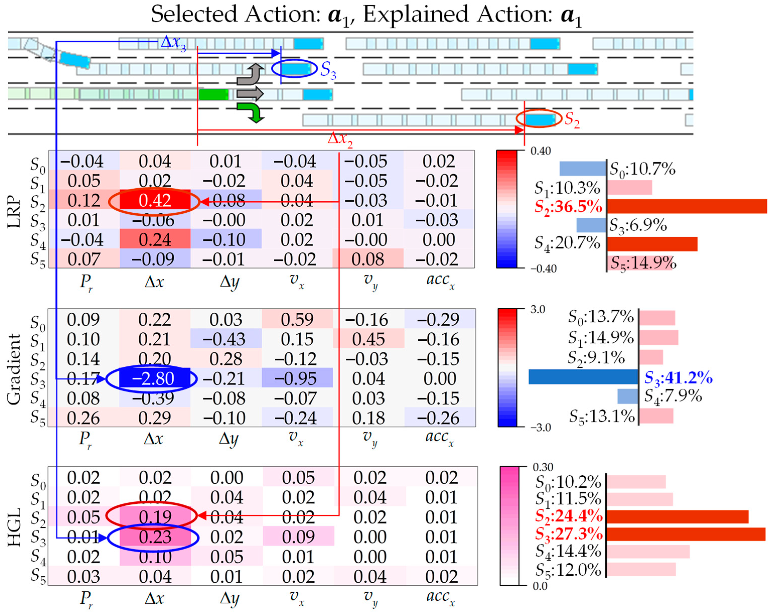
For qualitative analysis, two representative driving scenarios are randomly selected, and the decision-making behavior of the DRL agent is interpreted using LRP, Gradient, and HGL methods, as shown in Figure 6 and Figure 7. In the attribution heatmaps, the six rows correspond to the agent’s observation state. Specifically, the first row represents the ego vehicle state, while the second to sixth rows represent the states of surrounding vehicles. Each vehicle is described by six state features.

In the LRP heatmaps, red indicates features that make positive contributions to the current decision, blue denotes negative contributions, and white indicates negligible contributions near zero. These relevance values characterize the degree to which individual features support or oppose the current decision from a responsibility-allocation perspective. In contrast, the gradient-based saliency maps reflect the local sensitivity of the model output to input perturbations. In this case, red denotes positive gradients, indicating that increasing the feature value increases the predicted action advantage, whereas blue denotes negative gradients, indicating the opposite effect. In the HGL results, pink-colored features are highly relevant to the current decision, reflecting feature importance jointly inferred from local sensitivity (gradient-based attribution) and global contribution (LRP-based attribution). To facilitate object-level comparison of the overall influence of different vehicles, a vehicle-level importance bar is displayed on the right side of each heatmap. The vehicle-level importance is defined as the proportion of the sum of absolute attribution values across all features associated with that vehicle.

In Scenario 1 (Figure 6), the ego vehicle selects a₂ (keep lane), and we analyze the predicted Q-value for action a₀ (lane change left).

From the LRP heatmap, the longitudinal distance ($\mathrm{\Delta }{x}_3$) to the left-front vehicle ($S_3$) and the distance ($\mathrm{\Delta }{x}_4$) to the right-rear vehicle ($S_4$) show the strongest positive and negative contributions, respectively, indicating their critical supporting and opposing roles in the left lane-change decision. This is consistent with intuitive expectations: A large left-front distance ($\mathrm{\Delta }{x}_3$) implies sufficient space that encourages a left lane change, whereas a large right-rear distance ($\mathrm{\Delta }{x}_4$) favors a right lane change and thus suppresses the left lane-change option. For sufficiently distant vehicles, distance-related contributions become saturated. In contrast, gradient-based attribution exhibits significantly reduced sensitivity to these features ($\mathrm{\Delta }{x}_3$ and $\mathrm{\Delta }{x}_4$). Since small perturbations in saturated distance features produce negligible changes in the model output, their corresponding gradient magnitudes remain low.

Gradient-based attribution focuses on the right-front ($S_2$) and left-rear ($S_5$) vehicles, whose distances ($\mathrm{\Delta }{x}_2$ and $\mathrm{\Delta }{x}_5$) lie in the decision-sensitive region and thus exhibit large gradient magnitudes. From a driving perspective, a short left-rear distance ($\mathrm{\Delta }{x}_5$) directly affects the feasibility of a left lane change, as insufficient rear spacing increases collision risk. Similarly, the right-front distance ($\mathrm{\Delta }{x}_2$) influences the attractiveness of a right lane change option, which may compete with the left lane-change decision. Notably, these two sensitive features ($\mathrm{\Delta }{x}_2$ and $\mathrm{\Delta }{x}_5$) are not prominently highlighted in the LRP heatmap. In the present scenario, although the right-front and left-rear distances strongly influence the decision through local perturbations, their accumulated relevance remains limited, and thus they receive relatively low LRP attribution.

By integrating gradient-based sensitivity with LRP-based contribution, the proposed HGL method captures both saturated yet decisive features ($\mathrm{\Delta }{x}_3$ and $\mathrm{\Delta }{x}_4$) and highly sensitive features ($\mathrm{\Delta }{x}_2$ and $\mathrm{\Delta }{x}_5$), thereby providing more comprehensive explanations and better alignment with human driving semantics.

In Scenario 2 (Figure 7), the ego vehicle selects a₁ (lane change right), and we analyze the predicted Q-value for action a₁ (lane change right).

Similar to Scenario 1, LRP highlights features with strong cumulative contributions, such as the longitudinal distance ($\mathrm{\Delta }{x}_2$) to the right-front vehicle ($S_2$), reflecting responsibility-based decision support. Gradient attribution emphasizes features ($\mathrm{\Delta }{x}_3$) near decision boundaries, capturing local sensitivity to potential state changes. In contrast, HGL effectively integrates both perspectives. It simultaneously attends to decisive contributors and sensitive boundary feature ($\mathrm{\Delta }{x}_2$ and $\mathrm{\Delta }{x}_3$). As a result, HGL produces explanations that are more stable, focused, and semantically consistent with human driving intuition.

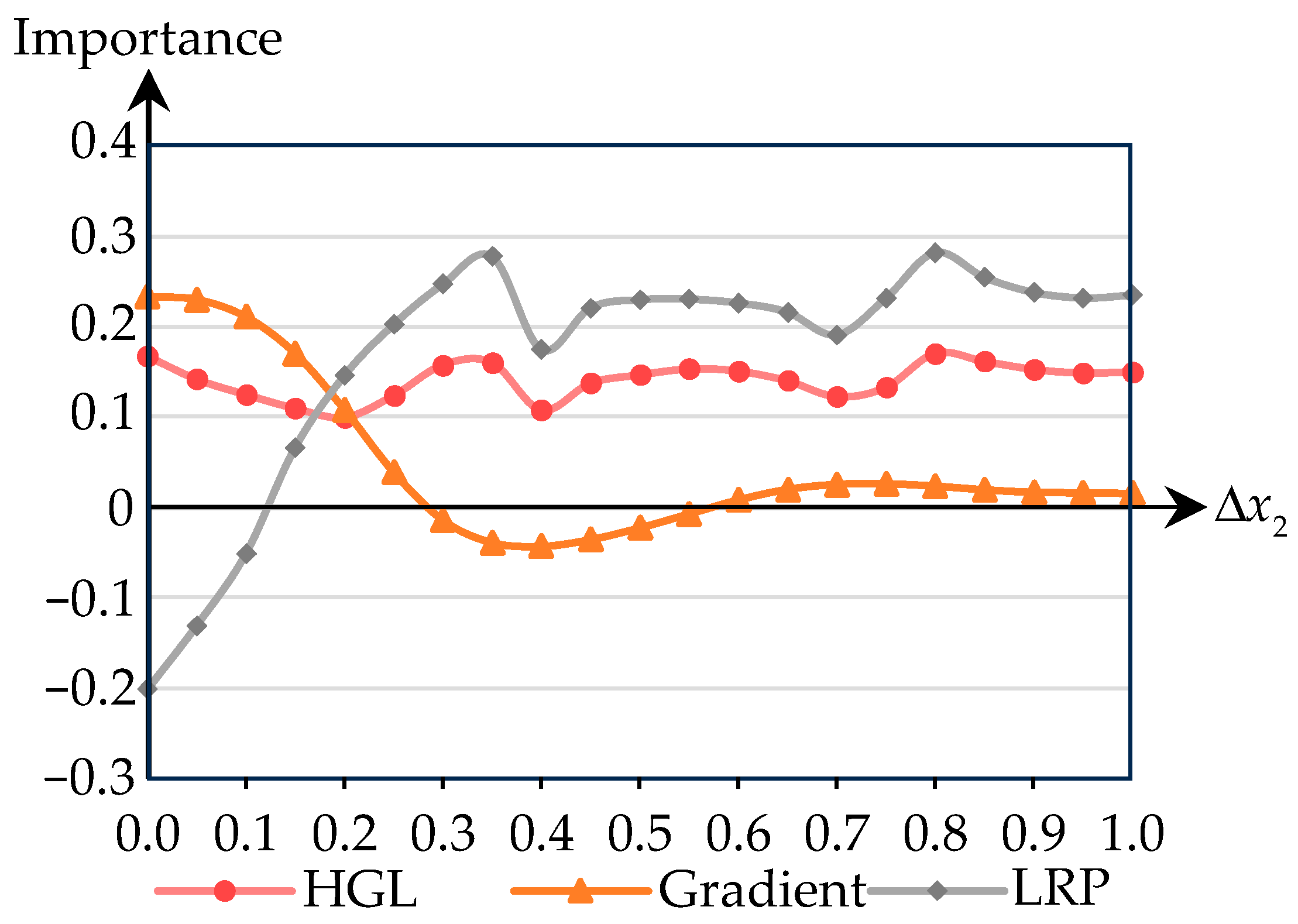
To further investigate the relationship between feature values and attribution importance, a counterfactual analysis is conducted based on Scenario 2 by systematically varying the value of $\mathrm{\Delta }{x}_2$. Attribution results are obtained using Gradient, LRP, and HGL, as illustrated in Figure 8.

The gradient-based results indicate that when $\mathrm{\Delta }{x}_2$ lies in the range of 0–0.2, the corresponding gradient magnitude is relatively large, reflecting the model’s high sensitivity to this feature. This behavior arises because the distance is small in this region, and minor perturbations can significantly influence the decision outcome. When $\mathrm{\Delta }{x}_2$ exceeds 0.2, the contribution of $\mathrm{\Delta }{x}_2$ gradually enters a saturation regime, and further variations have little effect on the model output, resulting in reduced gradient magnitude.

From the LRP perspective, when $\mathrm{\Delta }{x}_2$ falls within 0–0.05, the distance is excessively small and thus produces a strong negative contribution to the decision. Conversely, when $\mathrm{\Delta }{x}_2$ exceeds 0.2, LRP assigns a large positive relevance score, indicating that a sufficiently large right-front distance provides ample lane-change space and encourages a right lane change. In the intermediate interval of 0.05–0.2, however, LRP assigns only limited relevance, as the feature operates near the decision boundary where cumulative contribution is not yet dominant. Despite this, $\mathrm{\Delta }{x}_2$ remains highly influential in this region, and its importance cannot be effectively captured by LRP alone.

By jointly considering gradient-based local sensitivity and LRP-based global contribution, the proposed HGL method overcomes the limitations of individual attribution approaches. Across the entire range of the feature values ($\mathrm{\Delta }{x}_2$), HGL produces more comprehensive and stable attribution results, successfully identifying important features in both sensitivity-dominant regions near the decision boundary and contribution-dominant saturation regimes.

A comparison of Scenarios 1 and 2 further illustrates the reliability of the interpretation results under different driving situations. Although the surrounding traffic environments and driving decisions differ between the two scenarios, the attribution patterns consistently highlight the key vehicles influencing the decision-making process. In Scenario 1, the agent chooses to maintain its lane, and the interpretation mainly emphasizes the influence of nearby vehicles that constrain the ego vehicle’s motion. In contrast, Scenario 2 corresponds to a lane-changing decision, where the attribution results focus on vehicles in the adjacent lane that affect the safety and feasibility of the maneuver. Moreover, the two scenarios respectively reflect situations where potential risks originate from vehicles on the right and left sides, and the attribution results correctly assign higher importance to the corresponding vehicles. These results indicate that the proposed HGL attribution mechanism can consistently identify critical driving features across different traffic configurations and decision types, producing explanations that remain reasonable and semantically consistent with human driving intuition.

It is worth noting that the interpretability mechanisms employed in this study introduce minimal computational overhead. Both gradient-based attribution and LRP are implemented through a single backward pass, and the proposed HGL method reuses these computations without requiring additional iterative optimization. As a result, explanation generation can be performed efficiently based on the current decision state, making the approach suitable for real-time analysis in practical autonomous driving scenarios.

4.2. Global Explanation Analysis

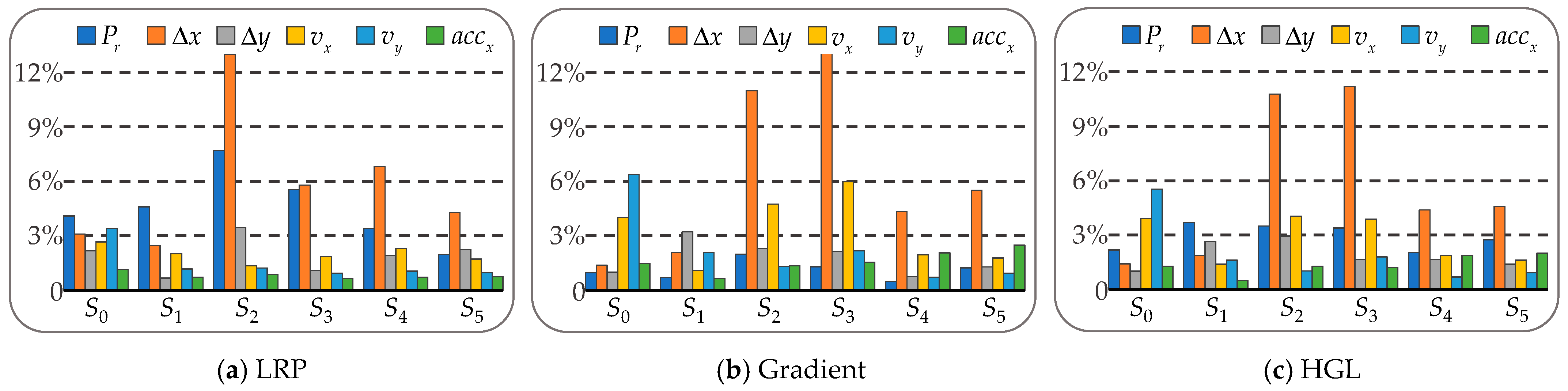
To obtain a global-level interpretation of the decision-making behavior, a total of 4000 samples are randomly selected for analysis. For each sample, different attribution methods are applied to interpret the model’s decisions, and feature importance is subsequently aggregated. Specifically, the absolute attribution values of each feature are averaged over all actions to quantify its overall importance. The resulting global feature importance distributions are shown in Figure 9.

From the global explanation results, both LRP and gradient-based attribution exhibit a certain degree of consistency in identifying key features. In particular, both methods recognize the longitudinal distances ($\mathrm{\Delta }{x}_2$ and $\mathrm{\Delta }{x}_3$) to the right-front ($S_2$) and left-front ($S_3$) vehicles as critical factors influencing lane-change decisions. However, notable differences remain in how different types of features are emphasized and interpreted, which can be attributed to the distinct attribution mechanisms underlying each method.

As shown in Figure 9a, the relevance-based LRP method assigns high importance not only to continuous state features but also to vehicle existence indicators (P_r). This behavior can be explained by the relevance conservation principle of LRP: the model output is treated as the total amount of decision responsibility, which is redistributed based on the cumulative contribution of each feature. Consequently, even discrete or bounded features may receive substantial relevance if they play a triggering or constraining role in the decision-making process.

In contrast, gradient-based attribution focuses on local first-order sensitivity, characterizing the instantaneous response of the model output to input perturbations, as illustrated in Figure 9b. For non-continuous features or features with limited variation ranges (e.g., vehicle existence indicators P_r), the gradients are typically close to zero and thus naturally down-weighted or ignored. On the other hand, for continuous dynamic features such as vehicle velocities, gradient attribution more accurately reflects the direction and magnitude of feature influence on the decision output. As a result, stronger sensitivity responses are observed for the velocities of surrounding vehicles (v_x), whereas LRP exhibits relatively unstable relevance allocation for these features.

By integrating these complementary attribution signals at the feature level, the proposed HGL method preserves both the common feature ($\mathrm{\Delta }{x}_2$ and $\mathrm{\Delta }{x}_3$) focus shared by different attribution methods and their respective strengths. Specifically, it maintains reliable interpretability for discrete features (P_r) while retaining sensitivity-consistent explanations for continuous dynamic features (v_x). As a result, HGL achieves more stable and semantically aligned global interpretability outcomes.

4.3. Summary of Experimental Results

In summary, the experimental results demonstrate that HA-IDRL achieves competitive decision-making performance while significantly improving interpretability. Across different traffic density conditions, the proposed method consistently attains performance comparable to representative DRL baselines, indicating that enhanced interpretability does not compromise decision quality.

From the perspective of local explanation analysis, gradient-based attribution mainly captures feature sensitivity and emphasizes dynamic variables that strongly influence the model output, while LRP focuses on contribution propagation and highlights features that make strong positive or negative contributions to the decision outcome. By integrating these complementary characteristics, the proposed HGL attribution mechanism captures a broader set of critical driving features and provides more comprehensive explanations that better align with human driving semantics.

The counterfactual attribution analysis further supports these observations. When analyzing the same key feature under different perturbation conditions, LRP tends to dominate in contribution-saturated regions where the feature strongly determines the decision outcome, whereas gradient-based attribution becomes more sensitive in intermediate regions where small feature variations significantly influence the model output. Consequently, the HGL mechanism produces more stable attribution results under different counterfactual perturbations, indicating stronger robustness of the generated explanations.

From the perspective of global explanation analysis, the results further reveal complementary characteristics between the two attribution methods. LRP tends to highlight features that make significant positive or negative contributions to the decision outcome, including discrete or bounded variables, such as vehicle existence indicators. In contrast, gradient-based attribution is more sensitive to continuous dynamic variables, such as vehicle speed, and more accurately reflects how small variations in these features influence the model output. By integrating these complementary properties, the HGL mechanism produces more comprehensive and semantically consistent explanations across different driving scenarios.

5. Conclusions

This paper addresses the critical challenge of interpretability in DRL-based autonomous driving behavior decision-making. While existing DRL approaches have demonstrated strong decision performance, their opaque internal mechanisms limit trustworthiness, safety validation, and practical deployment in safety-critical driving scenarios.

To bridge this gap, we proposed an HA-IDRL framework. The framework enhances interpretability at multiple levels without compromising decision performance. At the structural level, KAN is integrated into the Dueling DQN architecture to provide explicit nonlinear functional representations that are inherently aligned with attribution propagation. At the feature level, a novel HGL attribution method is introduced to jointly model local sensitivity and global contribution, thereby providing more comprehensive and human-intuitive explanations across both sensitive and saturated decision regions.

Extensive experiments on a highway lane-changing task using the highway-env simulator demonstrate that HA-IDRL achieves decision-making performance comparable to representative DRL baselines, including Dueling DQN and SAC. More importantly, the proposed method significantly improves the stability and semantic consistency of explanations in both local and global analyses. Compared with single-method attribution approaches, HGL integrates complementary attribution mechanisms, resulting in more comprehensive and stable explanations that better align with human driving intuition and decision semantics. In addition, the attribution process requires only a single backward propagation step, introducing minimal computational overhead and enabling efficient, real-time explanation generation.

Overall, this work demonstrates that high-performance autonomous driving decision-making and rigorous interpretability are not mutually exclusive. By integrating structural interpretability and hybrid attribution mechanisms, HA-IDRL provides a practical, scalable pathway to trustworthy DRL-based driving policies, facilitating transparent decision analysis and safer system validation.

The main contributions of this work can be summarized as follows. First, we extend gradient-based sensitivity analysis to the KAN-based value function and integrate it with LRP-based contribution allocation to develop a hybrid attribution mechanism that provides computationally efficient and semantically consistent explanations for DRL decision-making. Second, we introduce Kolmogorov–Arnold Networks (KANs) into the Dueling DQN framework to enhance structural interpretability and improve the consistency of attribution propagation. Finally, we validate the proposed HA-IDRL framework on a highway lane-changing task, demonstrating that it achieves competitive driving performance while significantly improving interpretability quality.

Future work will focus on extending the proposed interpretability framework from single-step decision explanations to temporal, multi-step decision processes, enabling analysis of how feature contributions evolve over time. In addition, incorporating interpretability outputs into safety assessment, policy verification, and human–machine interaction represents a promising direction for deploying interpretable reinforcement learning in real-world autonomous driving systems.

References

1. Paden, B.; Čáp, M.; Yong, S.Z.; Yershov, D.; Frazzoli, E. A survey of motion planning and control techniques for self-driving urban vehicles. IEEE Trans. Intell. Veh. 2016, 1, 33–55. [Google Scholar] [CrossRef] [Scilit]
2. Chen, X.; Xi, Z.; Xu, Y.; Xiong, Z.; Ding, X.; Wang, H. Balancing safety and efficiency for autonomous vehicles at urban uncontrolled crosswalk: Challenges and countermeasures. Accid. Anal. Prev. 2025, 220, 108111. [Google Scholar] [CrossRef] [Scilit] [PubMed]
3. Kurt, A.; Özgüner, Ü. Hierarchical finite state machines for autonomous mobile systems. Control. Eng. Pract. 2013, 21, 184–194. [Google Scholar] [CrossRef] [Scilit]
4. Dolgov, D.; Thrun, S.; Montemerlo, M.; Diebel, J. Path planning for autonomous vehicles in unknown semi-structured environments. Int. J. Robot. Res. 2010, 29, 485–501. [Google Scholar] [CrossRef] [Scilit]
5. Kesting, A.; Treiber, M.; Helbing, D. General lane-changing model MOBIL for car-following models. Transp. Res. Rec. 2007, 1999, 86–94. [Google Scholar] [CrossRef] [Scilit]
6. Bojarski, M.; Del Testa, D.; Dworakowski, D.; Firner, B.; Flepp, B.; Goyal, P.; Jackel, L.D.; Monfort, M.; Muller, U.; Zhang, J.; et al. End to end learning for self-driving cars. arXiv 2016, arXiv:1604.07316. [Google Scholar] [CrossRef] [Scilit]
7. Codevilla, F.; Müller, M.; López, A.; Koltun, V.; Dosovitskiy, A. End-to-end driving via conditional imitation learning. In Proceedings of the 2018 IEEE International Conference on Robotics and Automation (ICRA), Brisbane, Australia, 21–25 May 2018; IEEE Press: New York, NY, USA, 2018; pp. 4693–4700. [Google Scholar]
8. Codevilla, F.; Lopez, A.M.; Koltun, V.; Dosovitskiy, A. On offline evaluation of vision-based driving models. In Proceedings of the European Conference on Computer Vision (ECCV), Munich, Germany, 8–14 September 2018; Springer: Berlin/Heidelberg, Germany, 2018; pp. 236–251. [Google Scholar]
9. Mnih, V.; Kavukcuoglu, K.; Silver, D.; Rusu, A.A.; Veness, J.; Bellemare, M.G.; Graves, A.; Riedmiller, M.; Fidjeland, A.K.; Ostrovski, G.; et al. Human-level control through deep reinforcement learning. Nature 2015, 518, 529–533. [Google Scholar] [CrossRef] [Scilit]
10. Van Hasselt, H.; Guez, A.; Silver, D. Deep reinforcement learning with double q-learning. In Proceedings of the AAAI Conference on Artificial Intelligence, Phoenix, AZ, USA, 12–17 February 2016; AAAI Press: Washington, DC, USA, 2016; Volume 30. [Google Scholar]
11. Wang, Z.; Schaul, T.; Hessel, M.; Hasselt, H.V.; Lanctot, M.; Freitas, N.D.; Claims, A.I. Dueling network architectures for deep reinforcement learning. In Proceedings of the International Conference on Machine Learning PMLR, New York, NY, USA, 20–22 June 2016; pp. 1995–2003. [Google Scholar]
12. Schulman, J.; Wolski, F.; Dhariwal, P.; Radford, A.; Klimov, O. Proximal policy optimization algorithms. arXiv 2017, arXiv:1707.06347. [Google Scholar] [CrossRef] [Scilit]
13. Haarnoja, T.; Zhou, A.; Abbeel, P.; Levine, S. Soft actor-critic: Off-policy maximum entropy deep reinforcement learning with a stochastic actor. In Proceedings of the International Conference on Machine Learning, PMLR, Stockholm, Sweden, 10–15 July 2018; pp. 1861–1870. [Google Scholar]
14. Shalev-Shwartz, S.; Shammah, S.; Shashua, A. Safe, multi-agent, reinforcement learning for autonomous driving. arXiv 2016, arXiv:1610.03295. [Google Scholar] [CrossRef] [Scilit]
15. Salmani Pour Avval, S.; Eskue, N.D.; Groves, R.M.; Yaghoubi, V. Systematic review on neural architecture search. Artif. Intell. Rev. 2025, 58, 73. [Google Scholar] [CrossRef] [Scilit]
16. Su, P.; Xiang, C.; Chen, D. Adopting graph neural networks to understand and reason about dynamic driving scenarios. IEEE Open J. Intell. Transp. Syst. 2025, 6, 579–589. [Google Scholar] [CrossRef] [Scilit]
17. Miao, Q.; Jia, L.; Xie, K.; Fu, K.; Yang, Z. A Comprehensive Survey and Taxonomy of Mamba: Applications, Challenges, and Future Directions. Inf. Fusion 2025, 130, 104094. [Google Scholar] [CrossRef] [Scilit]
18. Du, S.; Zhu, Z.; Wang, X.; Han, H.; Qiao, J. Real-time local path planning strategy based on deep distributional reinforcement learning. Neurocomputing 2024, 599, 128085. [Google Scholar] [CrossRef] [Scilit]
19. Fujimoto, S.; Chang, W.D.; Smith, E.; Gu, S.S.; Precup, D.; Meger, D. For sale: State-action representation learning for deep reinforcement learning. Adv. Neural Inf. Process. Syst. 2023, 36, 61573–61624. [Google Scholar]
20. Ali, Y.; Hussain, F.; Bliemer, M.C.J.; Zheng, Z.; Haque, M. Predicting and explaining lane-changing behaviour using machine learning: A comparative study. Transp. Res. Part C Emerg. Technol. 2022, 145, 103931. [Google Scholar] [CrossRef] [Scilit]
21. Arrieta, A.B.; Díaz-Rodríguez, N.; Del Ser, J.; Bennetot, A.; Tabik, S.; Barbado, A.; Garcia, S.; Gil-Lopez, S.; Molina, D.; Benjamins, R.; et al. Explainable Artificial Intelligence (XAI): Concepts, taxonomies, opportunities and challenges toward responsible AI. Inf. Fusion 2020, 58, 82–115. [Google Scholar] [CrossRef] [Scilit]
22. Hassija, V.; Chamola, V.; Mahapatra, A.; Singal, A.; Goel, D.; Huang, K.; Scardapane, S.; Spinelli, I.; Mahmud, M.; Hussain, A. Interpreting black-box models: A review on explainable artificial intelligence. Cogn. Comput. 2024, 16, 45–74. [Google Scholar] [CrossRef] [Scilit]
23. Harinarayan, R.R.A.; Shalinie, S.M. XFDDC: EXplainable Fault Detection Diagnosis and Correction framework for chemical process systems. Process Saf. Environ. Prot. 2022, 165, 463–474. [Google Scholar] [CrossRef] [Scilit]
24. Lisboa, P.J.G.; Saralajew, S.; Vellido, A.; Fernández-Domenech, R.; Villmann, T. The coming of age of interpretable and explainable machine learning models. Neurocomputing 2023, 535, 25–39. [Google Scholar] [CrossRef] [Scilit]
25. Mathew, D.E.; Ebem, D.U.; Ikegwu, A.C.; Ukeoma, P.E.; Dibiaezue, N.F. Recent emerging techniques in explainable artificial intelligence to enhance the interpretable and understanding of AI models for human. Neural Process. Lett. 2025, 57, 16. [Google Scholar] [CrossRef] [Scilit]
26. Goodfellow, I.; Bengio, Y.; Courville, A. Deep Learning; MIT Press: Cambridge, MA, USA, 2016. [Google Scholar]
27. Omeiza, D.; Webb, H.; Jirotka, M.; Kunze, L. Explanations in autonomous driving: A survey. IEEE Trans. Intell. Transp. Syst. 2021, 23, 10142–10162. [Google Scholar] [CrossRef] [Scilit]
28. Doshi-Velez, F.; Kim, B. Towards A Rigorous Science of Interpretable Machine Learning. arXiv 2017, arXiv:1702.08608. [Google Scholar] [CrossRef] [Scilit]
29. Bastani, O.; Kim, C.; Bastani, H. Interpreting blackbox models via model extraction. arXiv 2017, arXiv:1705.08504. [Google Scholar]
30. Bastani, O.; Inala, J.P.; Solar-Lezama, A. Interpretable, verifiable, and robust reinforcement learning via program synthesis. In xxAI—Beyond Explainable AI: International Workshop, Held in Conjunction with ICML 2020, Vienna, Austria, 18 July 2020, Revised and Extended Papers; Springer International Publishing: Cham, Switzerland, 2020; pp. 207–228. [Google Scholar]
31. Kenny, E.M.; Tucker, M.; Shah, J. Towards interpretable deep reinforcement learning with human-friendly prototypes. In Proceedings of the Eleventh International Conference on Learning Representations, Kigali, Rwanda, 1–5 May 2023. [Google Scholar]
32. Ribeiro, M.T.; Singh, S.; Guestrin, C. “Why should I trust you?” Explaining the predictions of any classifier. In Proceedings of the 22nd ACM SIGKDD International Conference on Knowledge Discovery and Data Mining, San Francisco, CA, USA, 13–17 August 2016; ACM: New York, NY, USA, 2016; pp. 1135–1144. [Google Scholar]
33. Scott M. Lundberg, S.M.; Lee, S.-I. A unified approach to interpreting model predictions. In Proceedings of the 31st International Conference on Neural Information Processing Systems (NIPS’17), Long Beach, CA, USA, 4–9 December 2017; Curran Associates Inc.: Red Hook, NY, USA, 2017; pp. 4768–4777. [Google Scholar]
34. Sundararajan, M.; Taly, A.; Yan, Q. Axiomatic attribution for deep networks. In Proceedings of the International Conference on Machine Learning, PMLR, Sydney, Australia, 6–11 August 2017; pp. 3319–3328. [Google Scholar]
35. Bach, S.; Binder, A.; Montavon, G.; Klauschen, F.; Müller, K.-R.; Samek, W. On pixel-wise explanations for non-linear classifier decisions by layer-wise relevance propagation. PLoS ONE 2015, 10, e0130140. [Google Scholar] [CrossRef] [Scilit] [PubMed]
36. Huang, J.; Zhou, R.; Li, M.; Li, H.; Liu, Y.; Song, X. From black-box to white-box: Interpretable deep reinforcement learning with Kolmogorov-Arnold networks for autonomous driving. Transp. Res. Part C Emerg. Technol. 2026, 182, 105386. [Google Scholar] [CrossRef] [Scilit]
37. Liu, Z.; Wang, Y.; Vaidya, S.; Ruehle, F.; Halverson, J.; Soljačić, M.; Hou, T.Y.; Tegmark, M. Kan: Kolmogorov-Arnold networks. arXiv 2024, arXiv:2404.19756. [Google Scholar]
38. Leurent, E. An Environment for Autonomous Driving Decision-Making[EB/OL]. GitHub Repository. 2018. Available online: https://github.com/eleurent/highway-env (accessed on 3 February 2026).
39. Wang, G.; Hu, J.; Li, Z.; Li, L. Harmonious lane changing via deep reinforcement learning. IEEE Trans. Intell. Transp. Syst. 2021, 23, 4642–4650. [Google Scholar] [CrossRef] [Scilit]
Figure 1. Interpretable deep reinforcement learning framework.
Applsci 16 03096 g001
Figure 2. Illustration of feature contributions. (a) Schematic relationship between a continuous state feature (e.g., the longitudinal distance to the front-right vehicle) and a decision output (e.g., right lane change). (b) Schematic comparison of gradient attribution and LRP for the same decision objective.
Applsci 16 03096 g002
Figure 3. Training Performance under High-Density Traffic Conditions. Different colored curves represent the mean training performance of different algorithms, and the shaded regions indicate the standard deviation. Subfigure (a) shows the reward over training episodes, (b) shows the average speed over training episodes, (c) shows the safety penalty over training episodes, and (d) shows the energy consumption penalty over training episodes.
Applsci 16 03096 g003
Figure 4. Training Performance under Low-Density Traffic Conditions. Different colored curves represent the mean training performance of different algorithms, and the shaded regions indicate the standard deviation. Subfigure (a) shows the reward over training episodes, (b) shows the average speed over training episodes, (c) shows the safety penalty over training episodes, and (d) shows the energy consumption penalty over training episodes.
Applsci 16 03096 g004
Figure 5. Training Performance under Medium-Density Traffic Conditions. Different colored curves represent the mean training performance of different algorithms, and the shaded regions indicate the standard deviation. Subfigure (a) shows the reward over training episodes, (b) shows the average speed over training episodes, (c) shows the safety penalty over training episodes, and (d) shows the energy consumption penalty over training episodes.
Applsci 16 03096 g005
Figure 6. Comparative attribution visualization in Scenario 1. The attribution results produced by LRP, Gradient, and HGL are presented for comparison. The red and blue ellipses and arrows highlight the consistent salient regions identified by different explanation methods.
Applsci 16 03096 g006
Figure 7. Comparative attribution visualization in Scenario 2. The attribution results produced by LRP, Gradient, and HGL are presented for comparison. The red and blue ellipses and arrows highlight the consistent salient regions identified by different explanation methods.
Applsci 16 03096 g007
Figure 8. Counterfactual Attribution.
Applsci 16 03096 g008
Figure 9. Comparison of global attribution explanations generated by different methods. (a) LRP-based global attribution explanation. (b) Gradient-based global attribution explanation. (c) HGL-based global attribution explanation.
Applsci 16 03096 g009