Zone-Based Interim Verification Method for 2D Vision Measurement Systems Using Non-Calibrated Artifacts: Performance, Spatial Consistency, and Future Applications

Abstract

This paper presents a zone-based method for the interim verification and spatial metrological characterization of a 2D vision measurement system. The approach relies on a system calibrated along a single axis and employs a stable yet non-calibrated artifact, demonstrating that spatial performance assessment can be achieved without the need for fully calibrated artifacts distributed across the entire field of view. To enable this process, a custom-designed reference standard was developed, providing a straightforward, robust, and cost-effective solution for performing interim verification tasks. The proposed method provides a structured framework for evaluating both precision and spatial consistency across the measurement surface, even in the absence of fully calibrated standards distributed across the surface. The method is applicable to a wide range of vision-based measurement systems, including those supporting industrial Optical Character Recognition (OCR), while maintaining alignment with established metrological principles. When combined with complementary optical performance tests, the approach supports robust and repeatable interim verification strategies in advanced manufacturing metrology.

1. Introduction

The objective of this work was to propose and evaluate a new method for the characterization and qualification of the entire measurement surface of a vision machine calibrated along only one axis.

Modern manufacturing increasingly requires agile, flexible and cost-effective verification methods that are capable of ensuring dimensional quality across a wide field of view and frequently changing configurations. As image-based measurement systems expand in scope, guaranteeing measurement precision and stability—without relying on cumbersome or time-consuming calibration procedures—has become essential.

Conventional calibration relies on standardized artifacts that must cover the entire measurement surface to enable complete system characterization. These artifacts are typically expensive, difficult to handle, and unsuitable for frequent interim checks or for systems that must be regularly reconfigured. Such constraints highlight the need for alternative strategies that are capable of maintaining metrological assurance without requiring fully calibrated standards across the whole field of view.

This work investigates the feasibility of a new method for zonal characterization and interim verification of the measurement surface of a vision machine calibrated along only one axis, using a non-calibrated yet stable artifact. The proposed approach enables global assessment of both measurement performance and precision across the entire field of view, reducing the dependency on fully traceable artifacts distributed across the surface. This provides a scalable, adaptable, and cost-effective solution for maintaining metrological quality in optical systems used in industrial and measurement environments [1,2].

While the method is general and applicable to a wide range of 2D vision systems [3,4,5], one relevant use case is the verification of cameras employed in Optical Character Recognition (OCR) [6,7,8,9,10,11,12,13,14,15,16]. OCR technologies are widely used in industrial inspection, product tracking, document verification, security applications, and automated quality control systems [9,10,11,12,13,14,15,16], where measurement reliability directly affects recognition accuracy and system robustness.

It should be emphasized that the objective of the proposed method is not to replace full metrological calibration procedures, but to provide a practical interim verification tool that is capable of detecting spatial variations in measurement performance across the field of view.

2. Materials and Methods

Some of the main metrology concepts are defined below:

We will refer to dispersion as the degree to which repeated measurement results vary from each other, quantified by statistical measures such as standard deviation [17].

Measurement uncertainty will be considered to be the parameter that describes the range within which the true value of the measurand is believed to lie [17].

Repeatability will be the closeness of agreement between successive measurements of the same quantity carried out under the same conditions: the same measurement method, same operator, same equipment, same location and a short time interval [17].

Error correction refers to the process of compensating for known systematic effects in the measurement system [17].

2.1. Materials

Following the terminology recommended in [18,19], the equipment used was as follows.

2.1.1. Digital Thermohygrograph

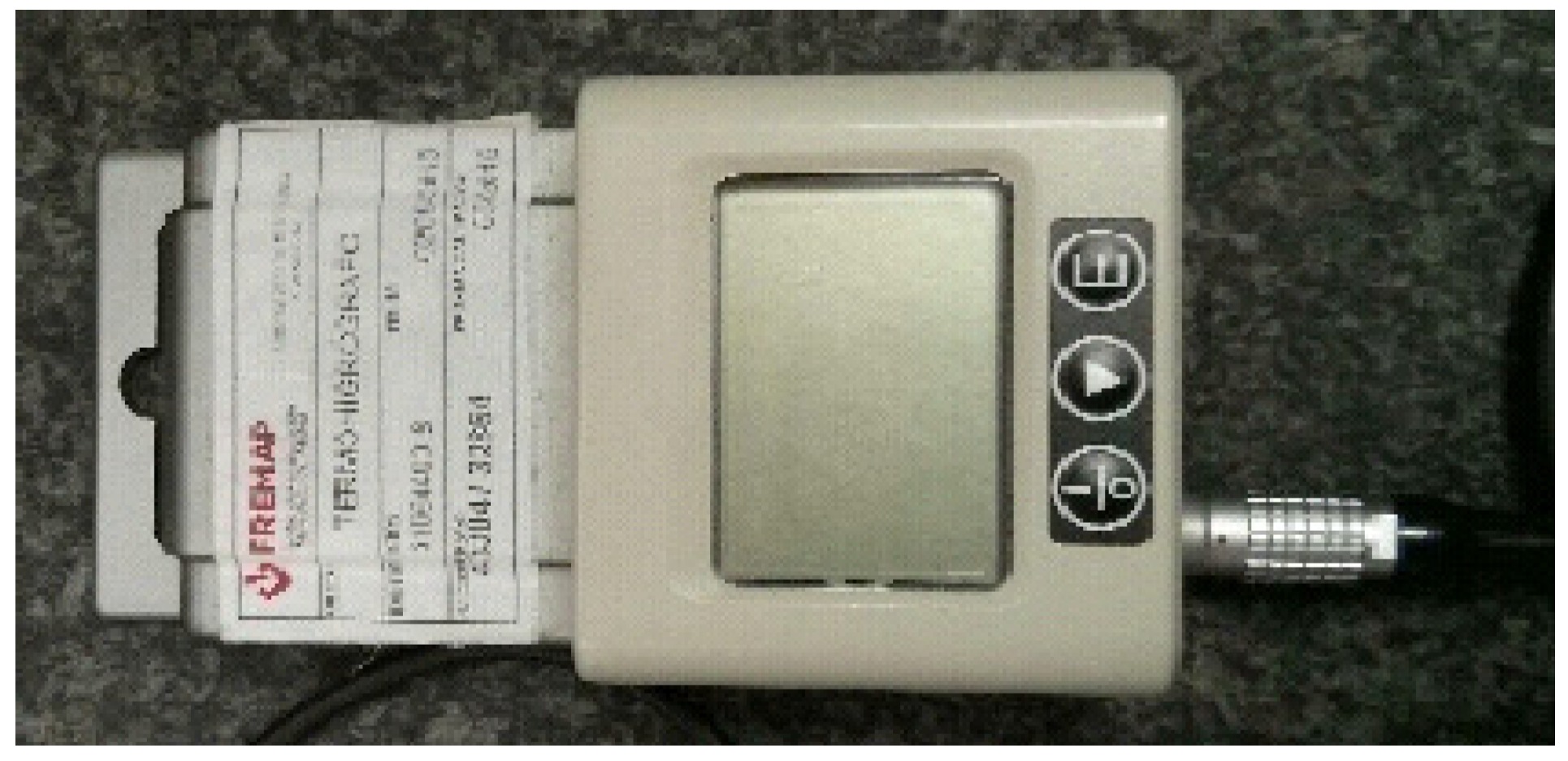
An auxiliary instrument was used to monitor the ambient temperature and relative air humidity (see Figure 1). These two parameters were measured using an external probe connected to the device, and the data were simultaneously recorded on a computer. It is suitable for the test, according to the specifications given in

Table 1. Thermohygrograph specifications.

Specifications
Brand	Testo (Titisee-Neustadt, Germany)
Model	Testostor Data Logger 171
Identification	43004
Measurement Range	Humidity: 0% to 100%
	Temperature: −35 °C to 70 °C
Scale Division	Humidity: 0.1%
	Temperature: 0.1 °C

.

Its maximum expanded uncertainty for the measurement of temperature was 0.17 °C and the relative humidity was below 1.3%.

The standardized temperature for this laboratory, accredited by ENAC, is 20 ± 1 °C, and humidity remains at 55 ± 10%.

2.1.2. Vision-Based Measurement System

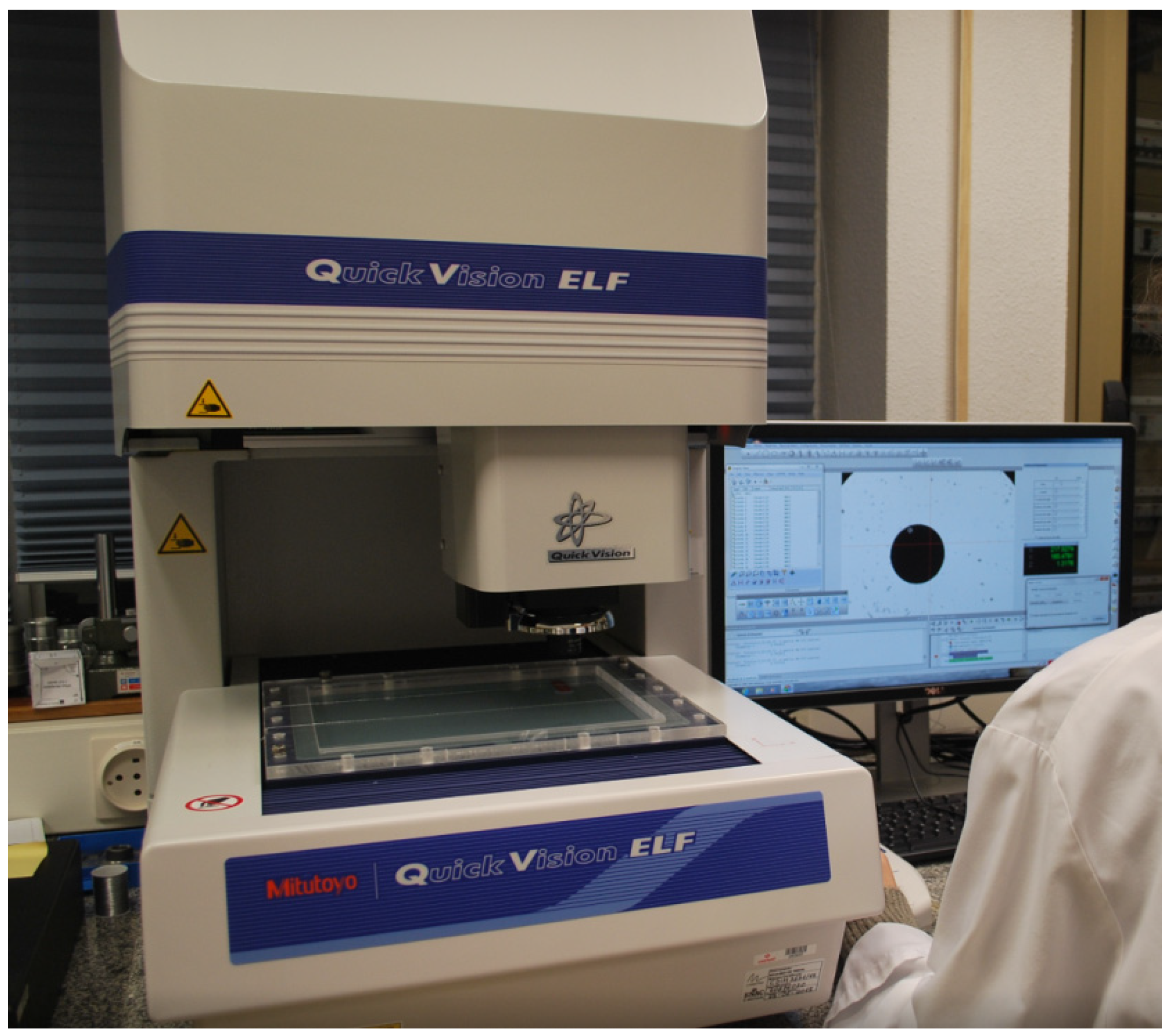
Using a CNC image processing measurement system (see Figure 2) offers 2.3 μm accuracy (for a length of 100 mm). It is an indirect measurement instrument that is capable of measuring both linear and curved dimensions.

It is suitable for the test following the specifications given in

Table 2. Quick Vision ELF vision machine specifications.

Specifications
Measurement Range X-Axis	0–250 mm
Measurement Range Y-Axis	0–200 mm
Measurement Range Z-Axis	0–200 mm
Resolution	0.1 µm/Reflective-type linear encoder
Max. Speed (X/Y/Z)	200 mm/s
PRL Illumination	Vertical reflection white LED light
	Coaxial white LED light
	Programmable white LED ring light
Glass Workpiece Size	312 × 269 mm
Max. Workpiece Load	33 lbs/15 kg
Main Unit and Stand Dimensions	847 × 586 × 528 mm (D × W × H)
Main Unit and Frame Weight	270 kg

.

Its calibration certificate reported an expanded uncertainty of 0.6 µm for the x and y axis, and 1.5 µm for the z axis.

2.1.3. Design and Description of the Uncalibrated Artifact

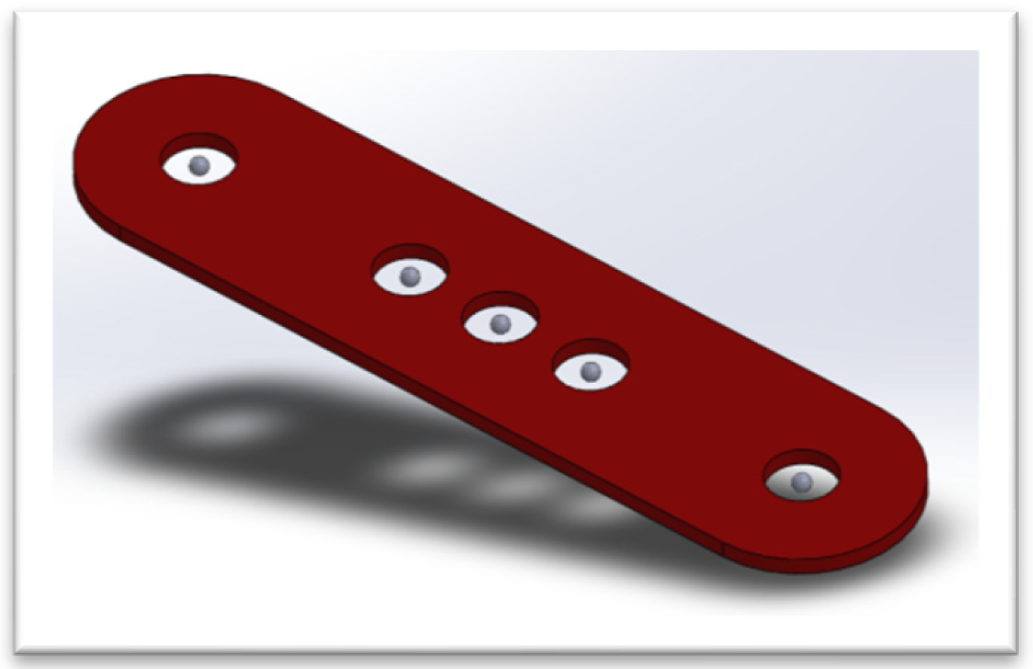
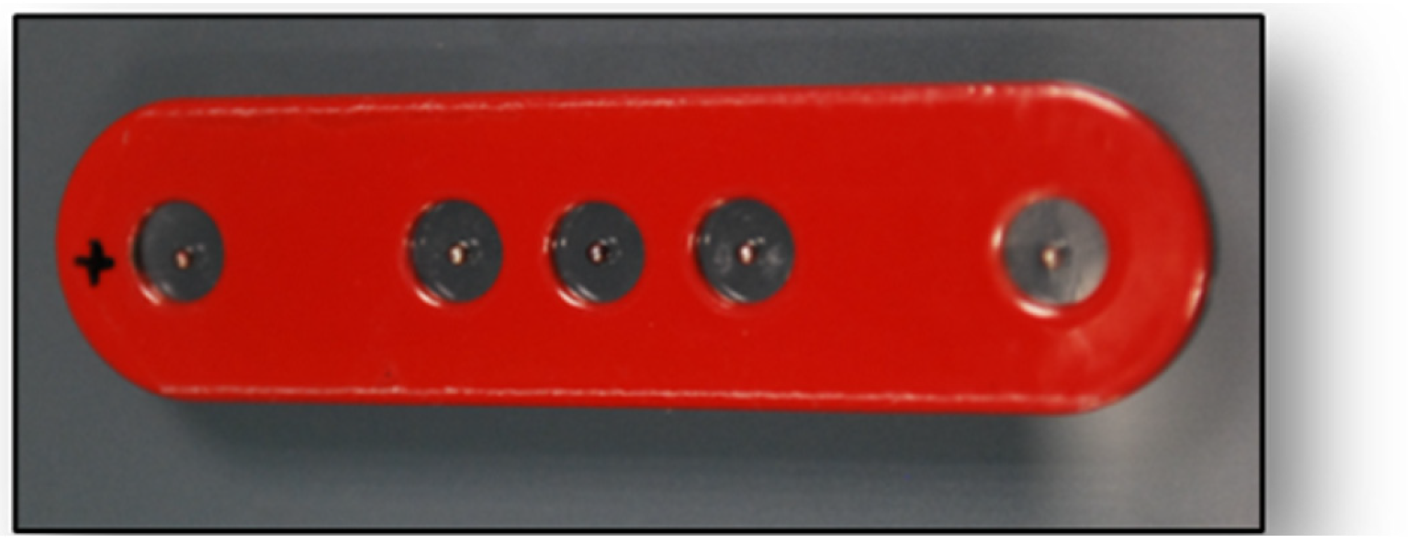
The uncalibrated artifact, specifically designed for the study, consisted of a painted metal support and five spheres approximately 1 mm in diameter. These were fixed in such a way that, despite not knowing their nominal dimensions, a comparative analysis could be performed, since the distances between them remained constant.

One of the measures implemented to ensure the stability of the artifact was the use of bearing-grade metal spheres, which provide excellent long-term stability and durability. The diameters of these spheres were measured in a separate test using a calibrated single-coordinate machine in the same laboratory, thus ensuring the level of stability required to verify the vision system. With regard to positional stability, the artifact itself was monitored over time. Any potential changes in the distances between spheres resulting from improper handling were found to be below the system’s resolution and therefore had a negligible impact on the verification process.

In any case, any observable change or suspicious deviation in any of the measured distances should prompt a calibration of the system using a certified standard. Consequently, this work demonstrates that a stable—though not calibrated—artifact is sufficient for performing intermediate verifications of the equipment between full calibrations.

This prototype (Figure 3, Figure 4 and Figure 5) has proven to be sufficiently robust for the study conducted, both due to the stability of the spheres’ positions and their sphericity, as well as their dimensions, which are suitable for measurement with the vision machine, and their maximum size, which is appropriate for the measurement field under consideration.

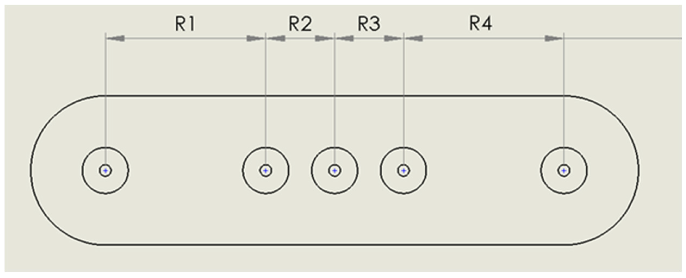
The distances used were designated as follows (Figure 4).

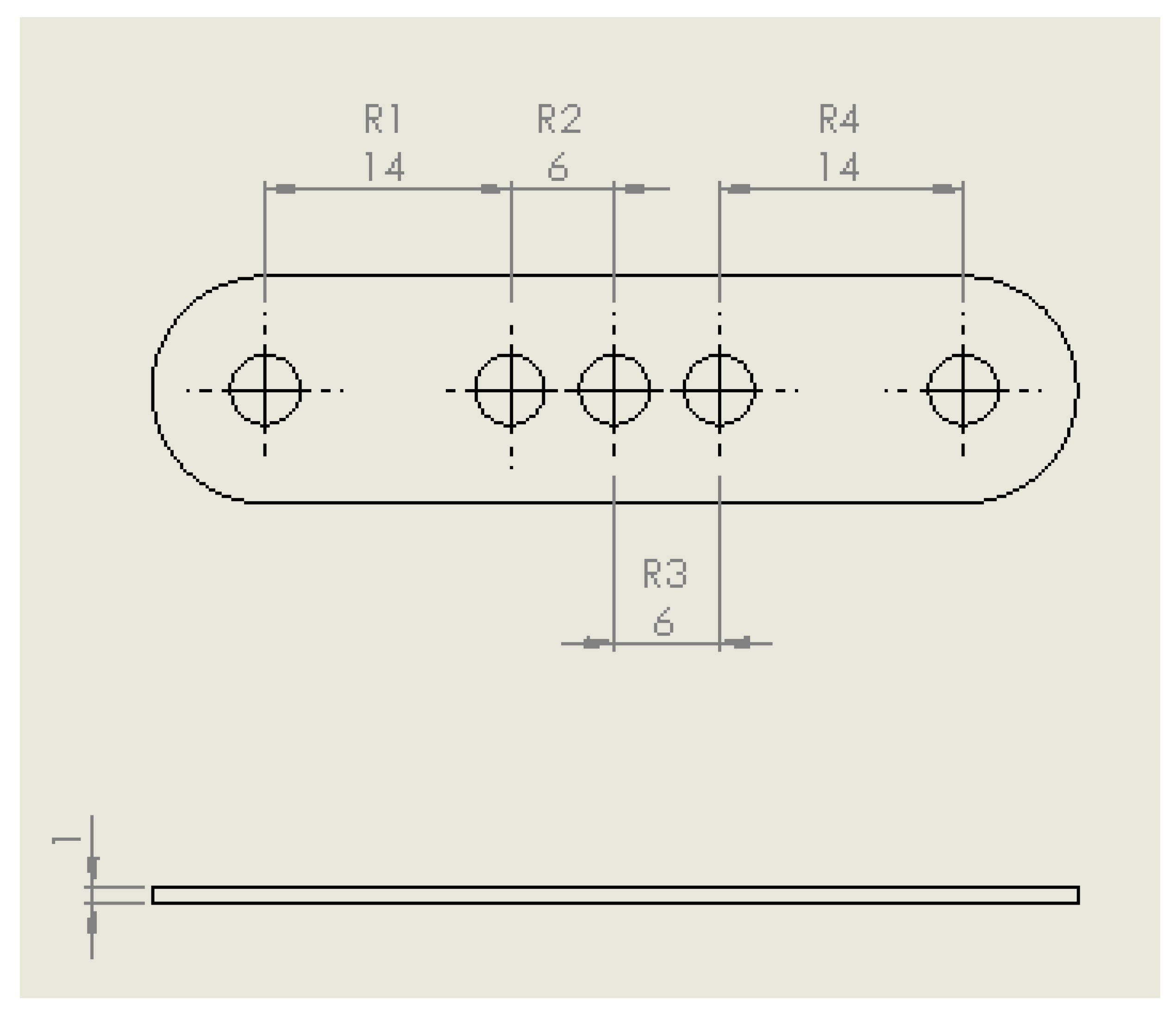
Appendix A includes the drawing of the specifically designed artifact.

2.1.4. Methacrylate Support

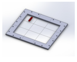
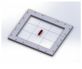
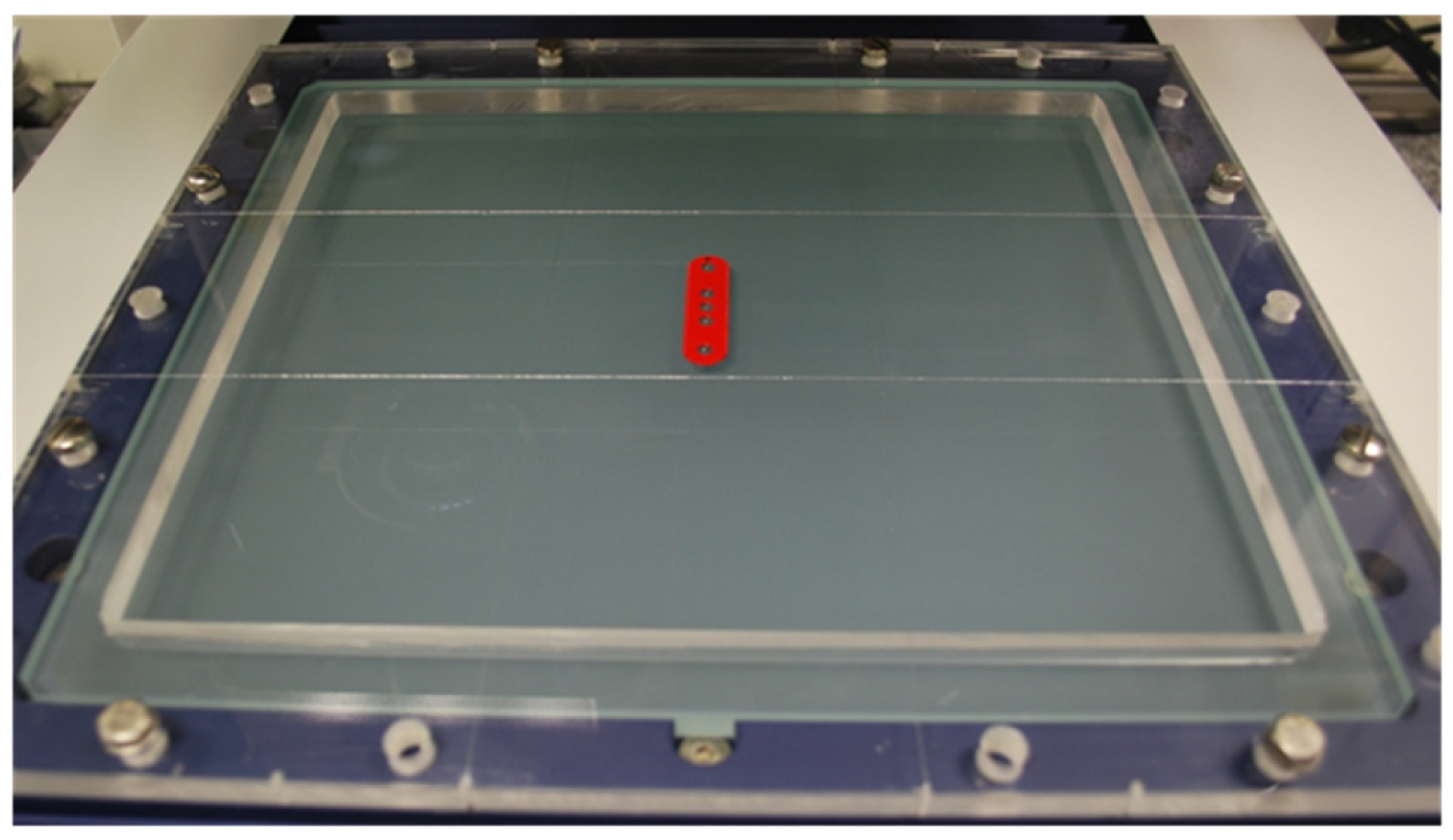
A methacrylate support was placed on the vision machine’s table to define the measurement zones (Figure 6).

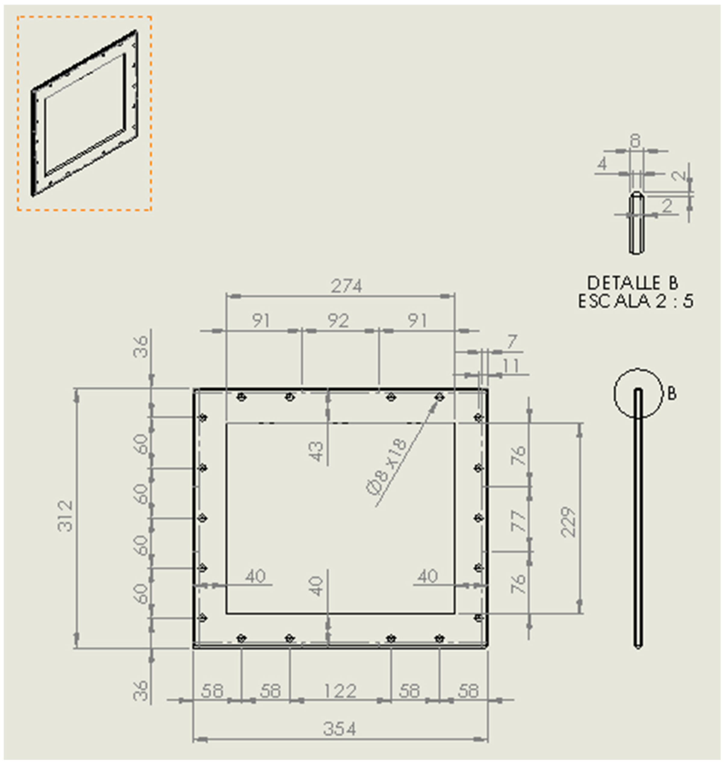
Appendix B includes the drawing of the specifically designed support.

2.2. Methods

The study was conducted following the guidelines provided in standards UNE-EN ISO 10360:2010 [20] and UNE-EN 15530:2011 [21], and the usual laboratory procedures [22].

2.2.1. Pre-Measurement Checks

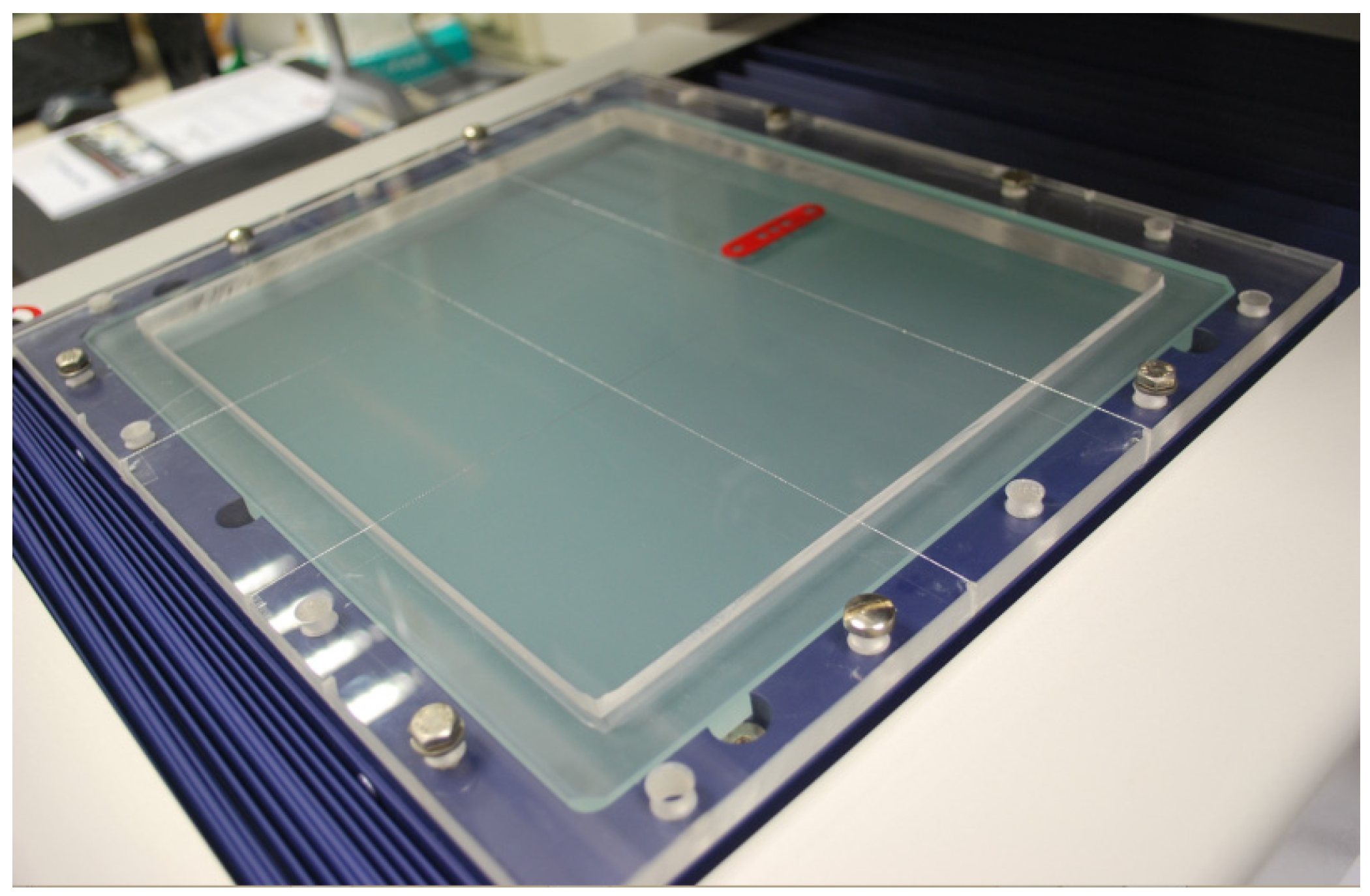
The methacrylate support was screwed onto the support of the vision machine surrounding the measurement area. This setup allowed for the measurement zones, which were distributed using a mesh layout, to be clearly defined (Figure 7 and Figure 8).

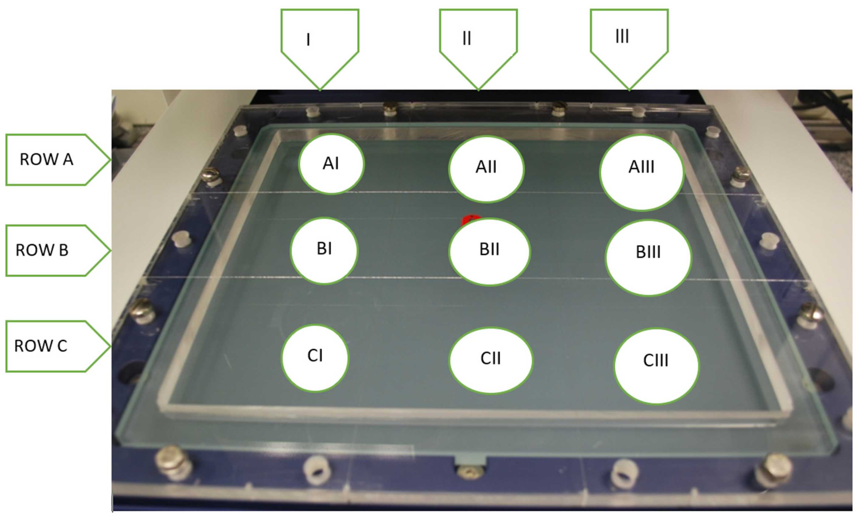
The following nomenclature was used (Figure 8).

The differentiation between zones was carried out using a 3 × 3 mesh with a methacrylate frame (see Appendix B) anchored to the support holding the screen, separating each zone with tensioned threads placed perpendicularly to each other.

To perform the measurements at each position, the device to be measured was manually placed, as shown in

Table 3. Measurement zones and nomenclature.

ROW	I	II	III
A
B
C

.

Note that each zone served as a reference that was intended to capture a measurement volume/surface as uniformly as possible within the machine’s measurement range. Each time the piece was placed in a given zone, its position was not exactly the same as the previous one. This does not affect the repeatability of the verification process.

If, during the application of this process, any type of anomaly was detected that could affect the operation of the measuring equipment, verification was stopped and restarted once the equipment was ready.

Before performing each measurement in each zone, the appropriate lighting adjustment and focusing were carried out.

2.2.2. Measurements

The temperature and humidity parameters used during the measurement were as follows (

Table 4. Environmental measurement conditions.

	Temperature
Initial temperature	19.9 °C
Final temperature	20.5 °C
Relative air humidity	47.8%

):

The diameters of the spheres Di (i = 1 to 5) were measured on the designed device in each of the positions.

The distances, Ri, to be measured were the separations between the centers of the previously mentioned spheres, Di. The machine detected the contour points of each sphere, and the obtained measurements corresponded to the distances between the centers of those circles.

Ri: distance between sphere i and i + 1.

These distances, Ri, were thus measured in 9 different positions within the measurement range of the vision machine, and in each position, measurements were taken 10 times.

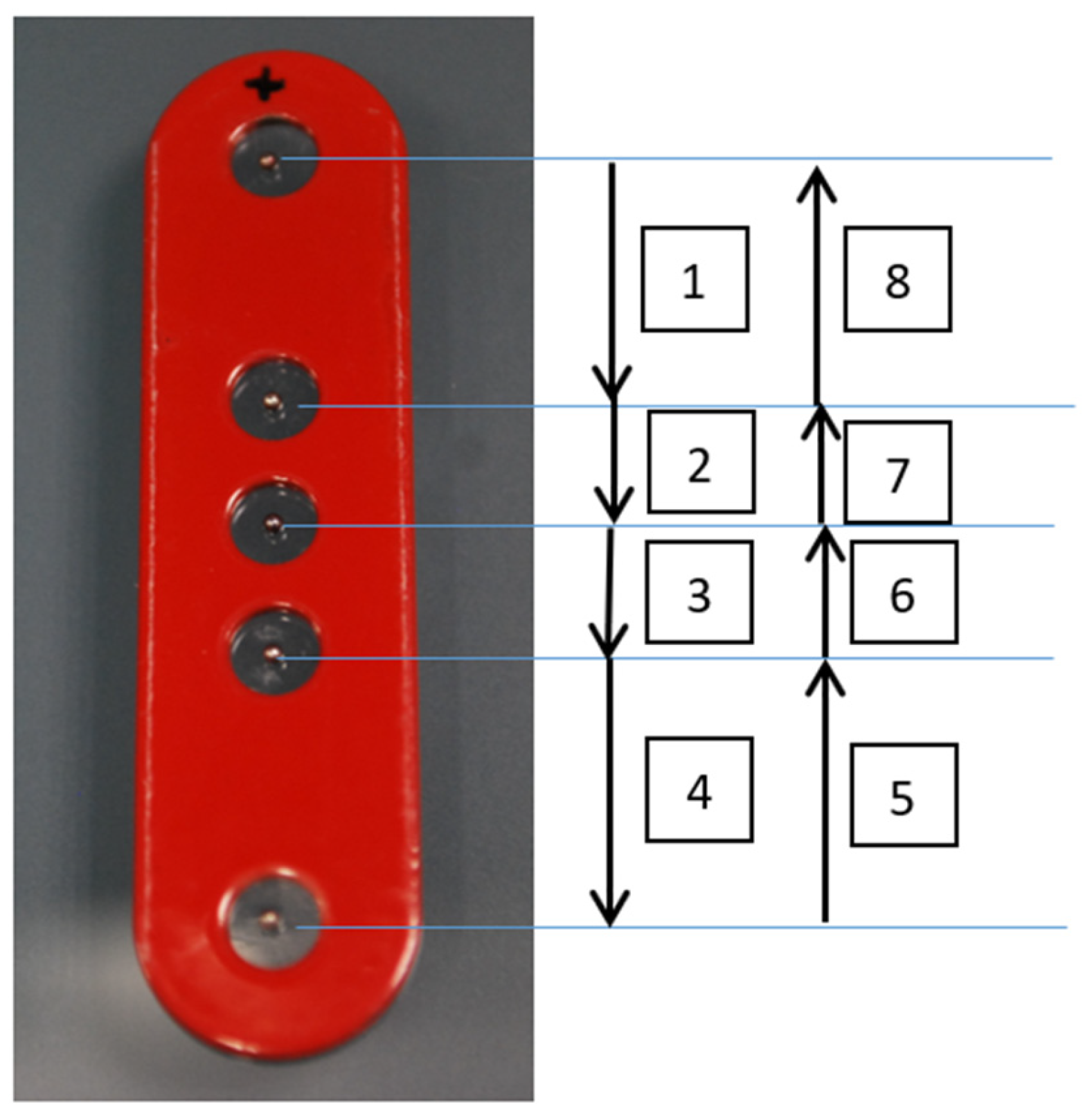
The first four measurements were taken in a downward direction, or descending. The last four were taken in the opposite direction, as shown in the following figure (Figure 9).

2.2.3. Measurement Acceptance or Rejection Criteria

It was agreed that the data obtained from the measurements taken at each calibration point corresponded to a normal or Gaussian distribution, although this might not always be the case. To determine whether the measurements were valid or needed to be repeated, the standard deviation was taken into account, as explained in the following section.

If, at a measurement point, the resulting standard deviation of all measurements exceeded the average scale division of the equipment, whether any error had occurred was verified during the measurements or in their transcription to the worksheet.

If, at a measurement point, the dispersion obtained exceeded three times the scale division, the measurements were repeated to rule out possible errors.

This is standard practice in the laboratory.

3. Results

The uncertainty analysis of the sphere diameters $D_i$ and inter-sphere distances $R_i$ follows the GUM approach, incorporating arithmetic and weighted means, repeatability, degrees of freedom, and both combined and expanded uncertainties. For each diameter, 45 measurements were performed across nine table positions in both manual and automatic modes, considering temperature effects, thermal gradients, and resolution limits. The resulting uncertainties, evaluated in the following sections, ranged between 0.2 and 0.4 µm. Distance measurements incorporated these diameter uncertainties, along with repeatability and environmental factors, leading to expanded uncertainties that were typically between 1 and 15 µm, depending on the zone and mode. Spatial analysis revealed that the vision system’s metrological behavior is non-uniform across the measurement surface: certain zones showed minimal dispersion, while others—especially position BII—displayed significantly degraded repeatability, independent of manual or automatic operation. Despite these spatial variations, all deviations remained within the global calibration uncertainty, validating the use of the uncalibrated artifact for interim verification.

Since the reference artifact is not dimensionally calibrated, the analysis focuses primarily on spatial consistency and repeatability, rather than absolute dimensional accuracy.

3.1. Uncertainty for Sphere Diameters, Di, and Distances, Ri

The basic parameters, calculated according to the GUM [23], were as follows:

• Arithmetic mean: Obtained by summing all the measurements of the same dimension and dividing the result by the number of values.
• Standard deviation of the mean of the measurements (dispersion): Represents the variability of the data with respect to the arithmetic mean, providing information about the repeatability of the measuring equipment.
• Weighted mean based on dispersion: Using the values of the same distance or diameter in each zone, the arithmetic mean and its dispersion were calculated. With the nine values (one per zone), a weighted mean was calculated based on their dispersion, so that zones with greater dispersion had less influence on the overall mean.
• Degrees of freedom (DoF) associated with each component according to [20].
• Combined uncertainty: Calculated as the root mean square of all contributions. Correlations between measurements were not considered necessary (ucomb).
• Expanded uncertainty: Uncertainty for a coverage factor of 95%, k = 2 (Uexp).

3.1.1. Uncertainty Associated with the Diameter of Each Sphere Di

We considered two cases: automatic measurements and manual measurements. In both cases, a total of 45 measurements were taken at the same horizontal position of the reference object, but in different zones of the measurement surface, thereby increasing the contribution.

Following the details provided at the beginning of this section, the components considered were:

• Weighted mean based on dispersion, calculated at each of the 9 positions (with five measurements taken at each point).
• Total repeatability of the 45 measurements, assuming a normal distribution and 44 degrees of freedom.
• Total contribution due to temperature, considering an uncertainty of 1 °C in temperature, assuming a rectangular distribution and a thermal expansion coefficient of 1.6 × 10⁻⁶, with 100 degrees of freedom.
• Total contribution due to thermal gradient, from the beginning to the end of the measurement process, with a variation of 0.5 °C, assuming a rectangular distribution and 100 degrees of freedom.
• Resolution, based on the last digit of the displayed values, assuming a rectangular distribution and 100 degrees of freedom.

A calculation was performed for each diameter, and the highest uncertainty between the manual and automatic cases was taken as the contribution to the measurement of the distance, Ri, between spheres Di and Di+1.

The results obtained for each diameter were as follows (

Table 5. Results of diameter measurements, uncertainties, and effective degrees of freedom.

	Mean (µm)	ucombined (µm)	DoF (ν)	Uexp (µm)
D1	996.7	0.2	44	0.4
D2	995.0	0.4	44	0.8
D3	999.9	0.2	44	0.3
D4	1000.6	0.2	44	0.5
D5	999.0	0.2	44	0.4

).

3.1.2. Uncertainty Associated with Each Distance, Ri

Following the details provided at the beginning of this section, the components considered were:

• Weighted mean based on dispersion, calculated at each of the 9 positions (with five measurements taken at each point).
• Total repeatability of the 45 measurements, assuming a normal distribution and 44 degrees of freedom.
• Contribution due to the uncertainty of the diameters of the involved spheres, previously obtained.

Therefore, this contribution will be directly considered as part of the distance measurement. The worst-case scenario would be that the uncertainties of the sphere centers add up as an error in the measurement. Thus, instead of “correcting,” we combine, and the uncertainty to be considered for each distance will be as it is possible to see in

Table 6. Contribution of the diameter to the uncertainty in the Ri distance.

Ri Distance	Involved Spheres	Considered Contribution ucombined	Degrees of Freedom (DoF)
R1	1 and 2	$\sqrt{u_{D1}^2+u_{D2}^2}=0.4 \mu \mathrm{m}$	67
R2	2 and 3	$\sqrt{u_{D2}^2+u_{D3}^2}=0.4 \mu \mathrm{m}$	61
R3	3 and 4	$\sqrt{u_{D3}^2+u_{D4}^2}=0.3 \mu \mathrm{m}$	81
R4	4 and 5	$\sqrt{u_{D4}^2+u_{D5}^2}=0.3 \mu \mathrm{m}$	88

(nomenclature of spheres are at Figure 5).

• Total contribution due to temperature, resulting from measuring with a temperature uncertainty of 1 °C, assuming a rectangular distribution, a thermal expansion coefficient of 1.6 × 10⁻⁶, and 100 degrees of freedom.
• Total contribution due to thermal gradient, from the beginning to the end of the measurement, with a variation of 0.5 °C, assuming a rectangular distribution and 100 degrees of freedom.
• Resolution, based on the last digit of the displayed values, assuming a rectangular distribution and 100 degrees of freedom.

The resulting uncertainties for all the distances are as follows (

Table 7. Uncertainty of the MANUAL Ri distance.

Ri Distance	Mean [mm]	ucombined [µm]	Degrees of Freedom (DoF)	Uexp [µm]
R1	12.789	0.6	125	1
R2	6.237	0.5	99	1
R3	6.4701	8	44	15.5
R4	12.548	0.9	60	2

and

Table 8. Uncertainty of the AUTO Ri distance.

Ri Distance	Mean [mm]	ucombined [µm]	Degrees of Freedom (DoF)	Uexp [µm]
R1	12.7894	0.6	278	1
R2	6.2373	5	45	10
R3	6.468	6	44	11
R4	12.550	0.9	60	2

).

3.2. Sphere Diameters Di

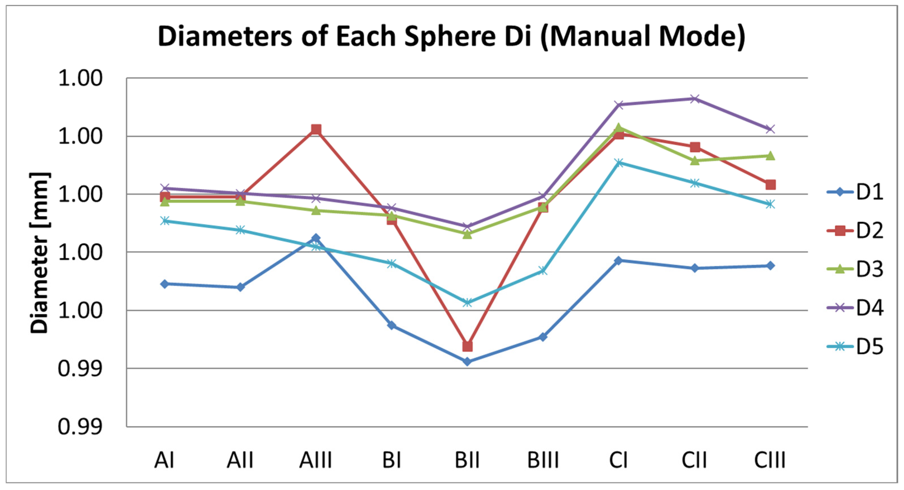
It can be observed in the following figure (Figure 10) that the diameter of the five spheres evolves in the same way throughout their placement on the measurement table, assessing the consistency of the measurement procedure.

Since the reference standard is the same but placed in different positions, this suggests that the algorithm depends on the position of the table, with maximum variations of

D4 pos CII − D4 pos BII = 4.397 µm

(1)

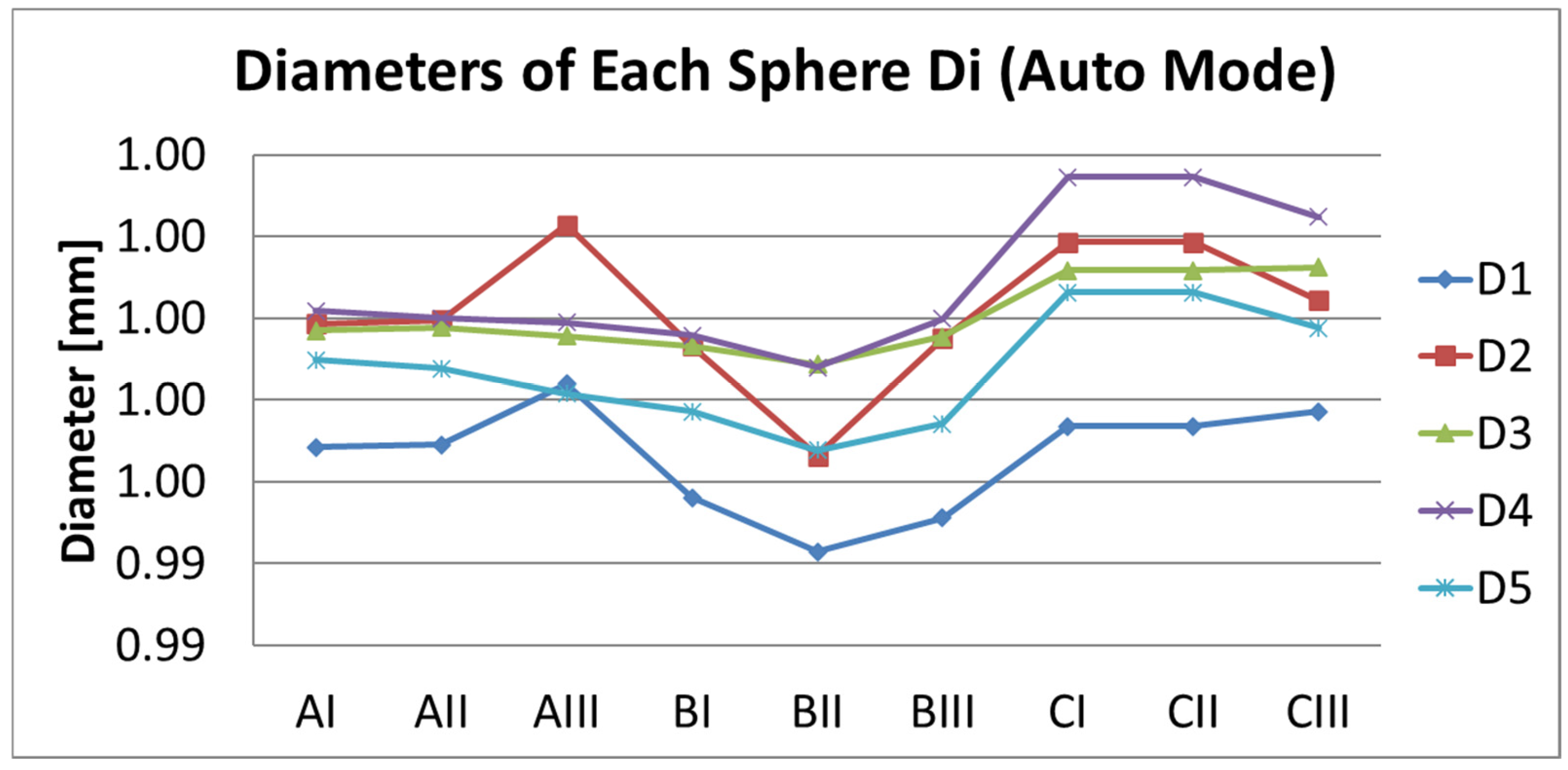
And exactly the same effect is observed in automatic mode, as shown in the following figure (Figure 11).

And the maximum variation becomes the following:

D4 pos CII − D4 pos BII = 4.666 µm

(2)

This variation may be due to:

• An error in the algorithm, via software. This seems unlikely.
• A variation in the focal position of a few microns that affects the relative position of the pattern, thus producing a seemingly larger reading, without being detected by the system’s resolution. Possibly due to a weight imbalance.

It is therefore highly advisable to measure the same pattern—such as the sphere—across the entire surface of the vision machine, in order to determine variations in its diameter, as shown in the following tables (

Table 9. Di in MANUAL mode along with its dispersion (mm).

		I [mm]	II [mm]	III [mm]
A	D1	0.997 ± 0.013	0.997 ± 0.024	0.998 ± 0.018
	D2	1.000 ± 0.033	1.000 ± 0.038	1.002 ± 0.048
	D3	1.000 ± 0.004	1.000 ± 0.011	0.999 ± 0.002
	D4	1.000 ± 0.006	1.000 ± 0.034	1.000 ± 0.005
	D5	0.999 ± 0.001	0.999 ± 0.003	0.998 ± 0.003
B	D1	0.995 ± 0.053	0.994 ± 0.030	0.995 ± 0.045
	D2	0.999 ± 0.012	0.995 ± 0.0001	1.000 ± 0.003
	D3	0.999 ± 0.017	0.999 ± 0.031	1.000 ± 0.007
	D4	1.000 ± 0.009	0.999 ± 0.082	1.000 ± 0.006
	D5	0.998 ± 0.009	0.996 ± 0.014	0.997 ± 0.002
C	D1	0.998 ± 0.074	0.997 ± 0.080	0.997 ± 0.190
	D2	1.002 ± 0.050	1.001 ± 0.050	1.000 ± 0.086
	D3	1.002 ± 0.047	1.001 ± 0.006	1.001 ± 0.018
	D4	1.003 ± 0.010	1.003 ± 0.014	1.002 ± 0.022
	D5	1.001 ± 0.016	1.001 ± 0.011	1.000 ± 0.015

The values showing the maximum (in red) and minimum (in blue) dispersion for each Di.

and

Table 10. Di in AUTO mode, along with its dispersion (mm).

		I [mm]	II [mm]	III [mm]
A	D1	0.997 ± 0.019	0.997 ± 0.031	0.998 ± 0.023
	D2	1.000 ± 0.014	1.000 ± 0.027	1.002 ± 0.044
	D3	1.000 ± 0.002	1.000 ± 0.012	1.000 ± 0.002
	D4	1.000 ± 0.011	1.000 ± 0.023	1.000 ± 0.001
	D5	0.999 ± 0.014	0.999 ± 0.007	0.998 ± 0.002
B	D1	0.996 ± 0.030	0.994 ± 0.038	0.995 ± 0.044
	D2	0.999 ± 0.008	0.997 ± 1.309	0.999 ± 0.014
	D3	0.999 ± 0.011	0.999 ± 0.014	0.999 ± 0.009
	D4	1.000 ± 0.008	0.999 ± 0.090	1.000 ± 0.017
	D5	0.998 ± 0.012	0.997 ± 0.028	0.997 ± 0.002
C	D1	0.997 ± 0.072	0.997 ± 0.072	0.998 ± 0.175
	D2	1.002 ± 0.032	1.002 ± 0.032	1.001 ± 0.080
	D3	1.001 ± 0.010	1.001 ± 0.010	1.001 ± 0.030
	D4	1.003 ± 0.015	1.003 ± 0.015	1.002 ± 0.005
	D5	1.001 ± 0.021	1.001 ± 0.021	1.000 ± 0.004

The values showing the maximum (in red) and minimum (in blue) dispersion for each Di.

):

This provides a qualitative indication of the condition of the measurement surface. This parameter is independent of the distance measurements.

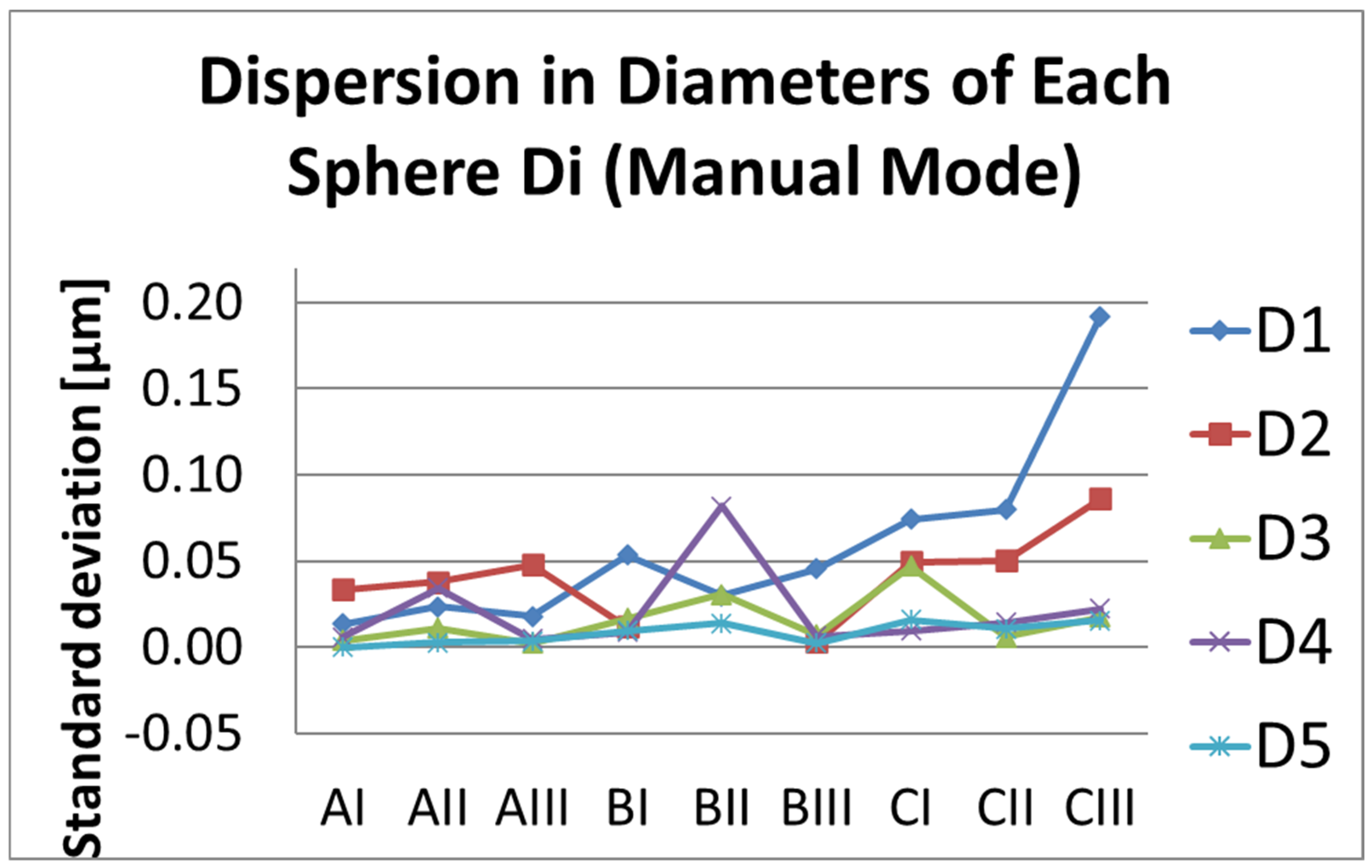
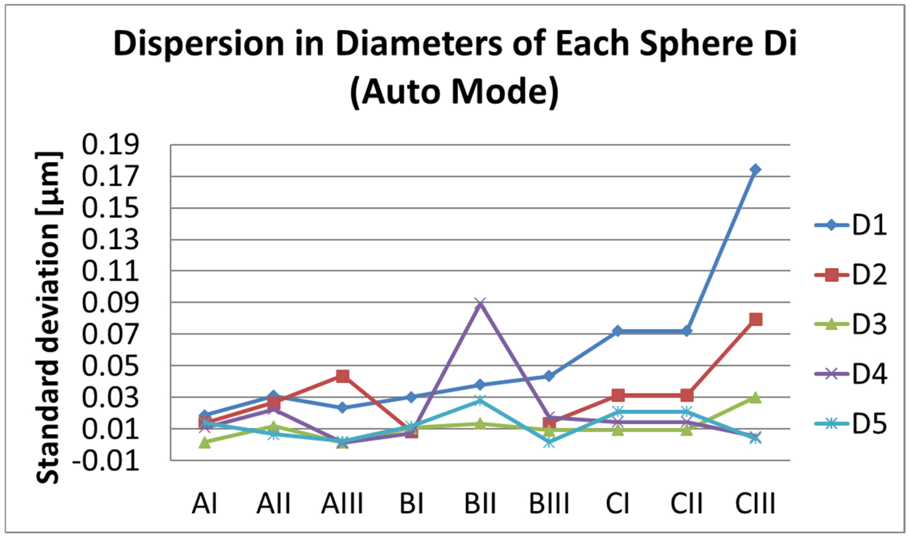
In the figures (Figure 12 and Figure 13) shown below, the diameter values (mm) of the spheres and their dispersion (mm) are indicated for each zone.

The diameter measurement D2 at position BII has been removed because both procedures result in significantly increased dispersion.

3.3. Ri Distances Between Spheres

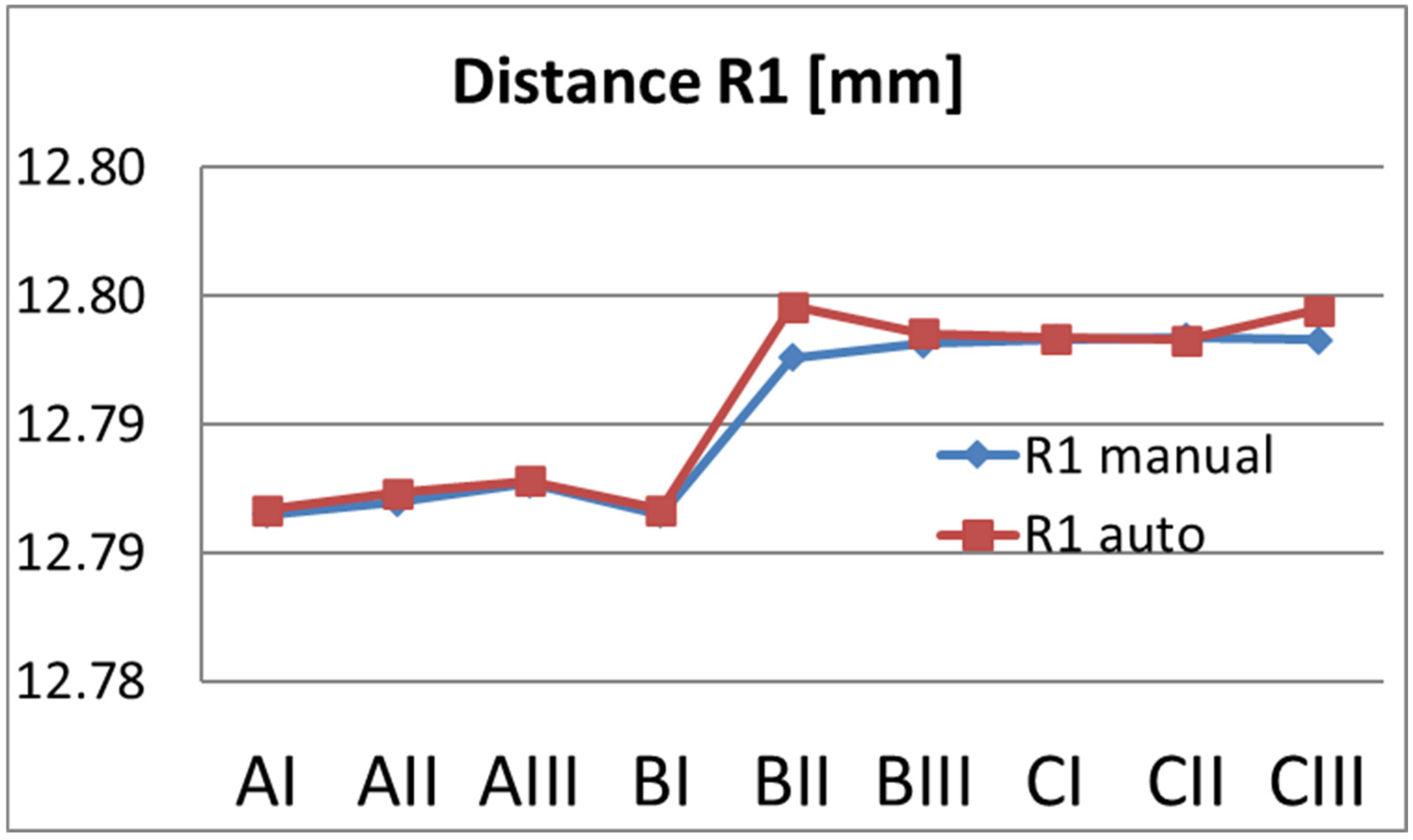
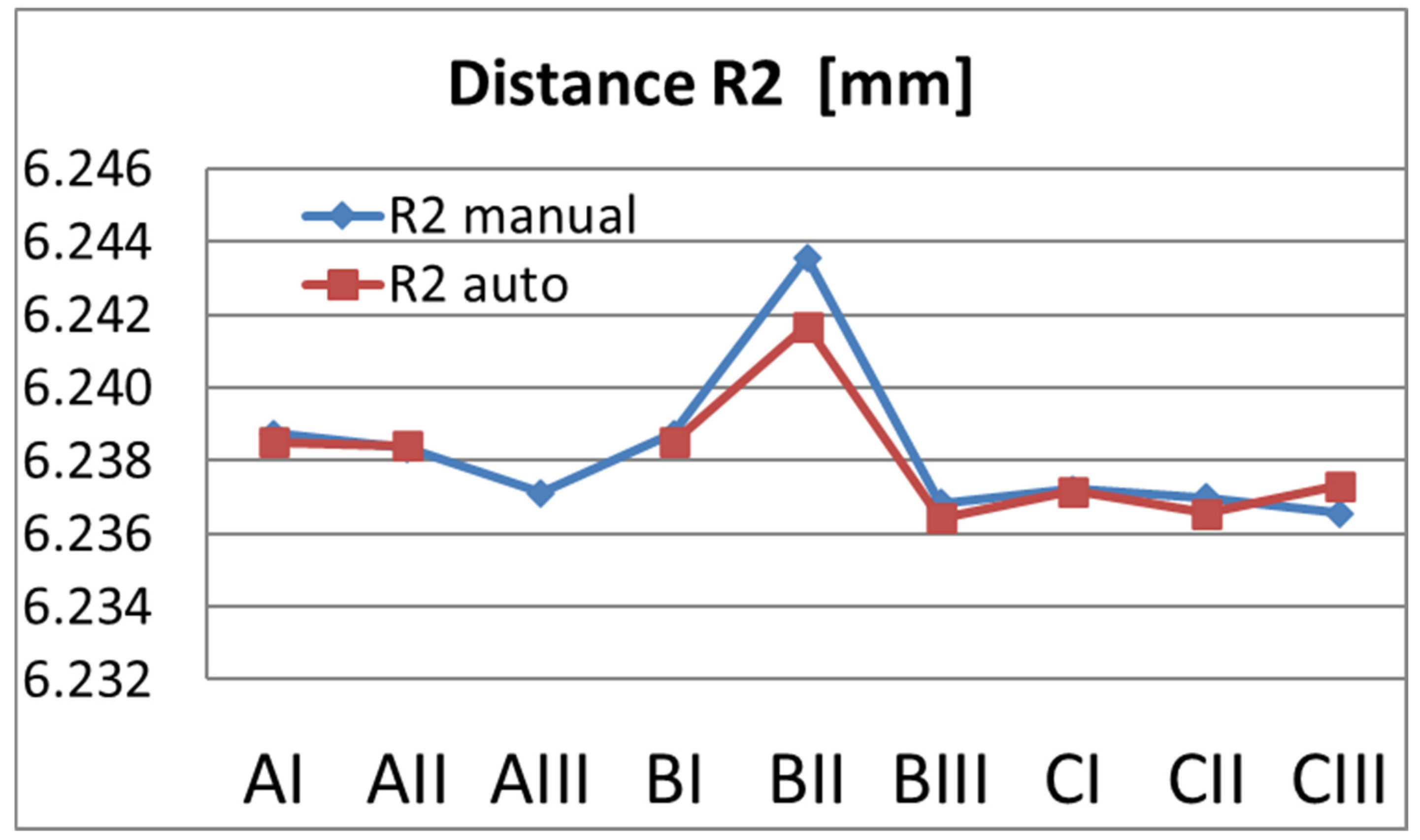
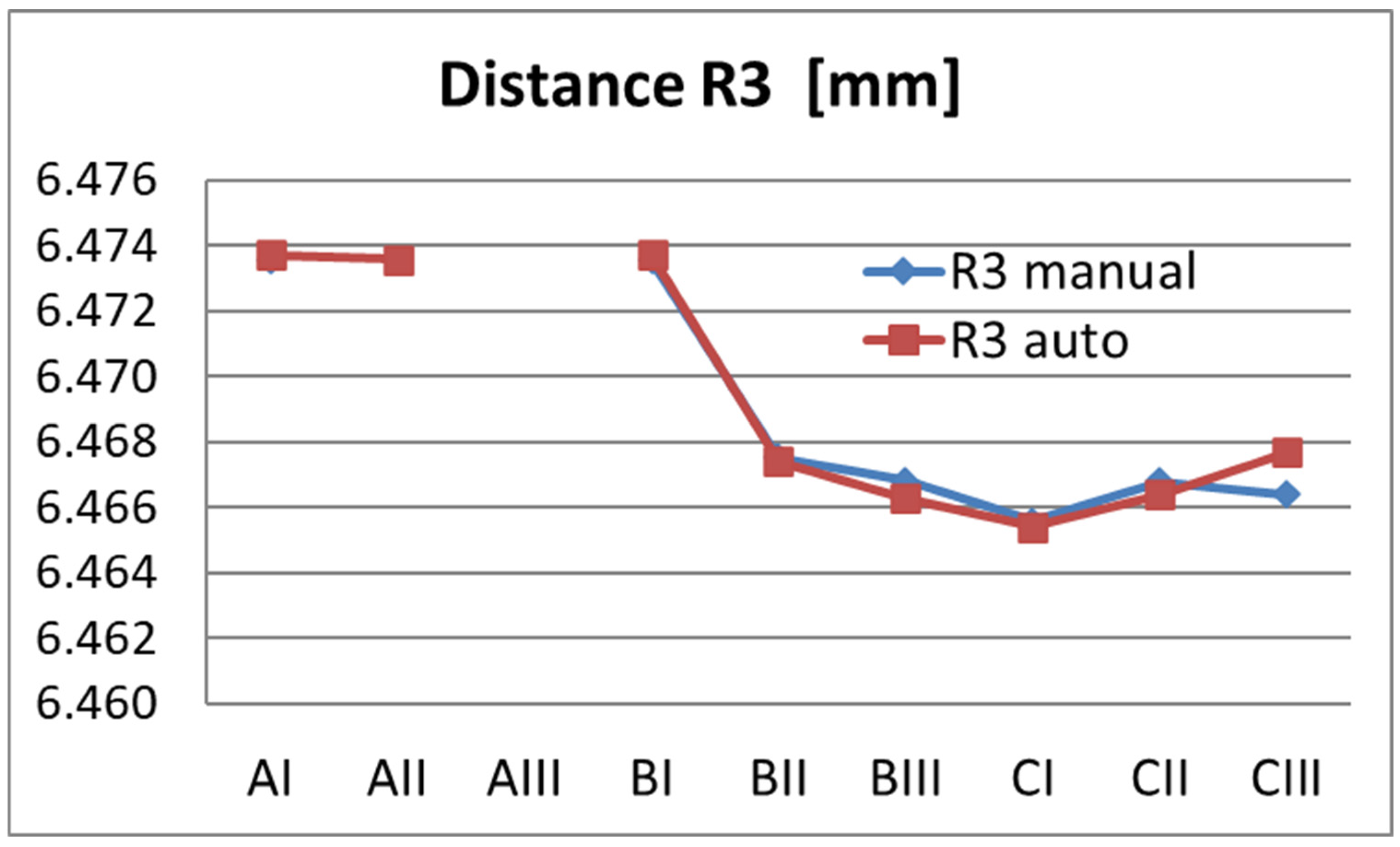
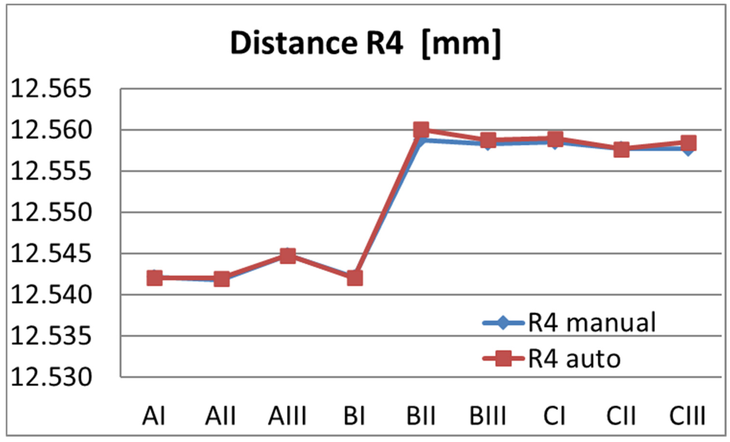
The non-calibrated artifact has been placed all over the measurement volume and each distance, Ri, has been measured with its own dispersion (see

Table 11. Ri in MANUAL mode along with its dispersion (mm).

		I [mm]	II [mm]	III [mm]
A	R1	12.786 ± 0.015	12.787 ± 0.016	12.788 ± 0.012
	R2	6.239 ± 0.015	6.238 ± 0.022	6.237 ± 0.010
	R3	6.474 ± 0.004	6.356 ± 39 **	6.356 ± 39 **
	R4	12.542 ± 0.004	12.542 ± 0.007	12.545 ± 0.002
B	R1	12.786 ± 0.015	12.793 ± 1.037 **	12.793 ± 0.022
	R2	6.239 ± 0.015	6.244 ± 1.173 **	6.237 ± 0.004
	R3	6.474 ± 0.004	6.468 ± 0.030	6.467 ± 0.007
	R4	12.542 ± 0.004	12.559 ± 0.040	12.559 ± 0.008
C	R1	12.793 ± 0.041	12.793 ± 0.032	12.793 ± 0.132
	R2	6.237 ± 0.014	6.237 ± 0.016	6.237 ± 0.011
	R3	6.466 ± 0.014	6.467 ± 0.012	6.466 ± 0.015
	R4	12.559 ± 0.011	12.558 ± 0.008	12.558 ± 0.009

The values showing the maximum (in red) and minimum (in blue) dispersion for each Ri. ** Anomalous values [mm] that are not taken into account.

and

Table 12. Ri in AUTO mode, along with its dispersion (mm).

		I [mm]	II [mm]	III [mm]
A	R1	12.787 ± 0.030	12.787 ± 0.015	12.788 ± 0.010
	R2	6.239 ± 0.026	6.238 ± 0.018	6.332 ± 38 **
	R3	6.474 ± 0.018	6.474 ± 0.018	6.356 ± 39 **
	R4	12.542 ± 0.011	12.542 ± 0.015	12.545 ± 0.002
B	R1	12.786 ± 0.030	12.794 ± 0.661	12.793 ± 0.027
	R2	6.239 ± 0.026	6.241 ± 0.762	6.236 ± 0.013
	R3	6.474 ± 0.018	6.467 ± 0.028	6.466 ± 0.017
	R4	12.542 ± 0.012	12.560 ± 0.046	12.559 ± 0.009
C	R1	12.793 ± 0.027	12.793 ± 0.032	12.794 ± 0.084
	R2	6.237 ± 0.007	6.237 ± 0.011	6.237 ± 0.009
	R3	6.466 ± 0.055	6.466 ± 0.015	6.468 ± 0.013
	R4	12.559 ± 0.054	12.558 ± 0.094	12.558 ± 0.008

The values showing the maximum (in red) and minimum (in blue) dispersion for each Ri. ** Anomalous values that are not taken into account.

):

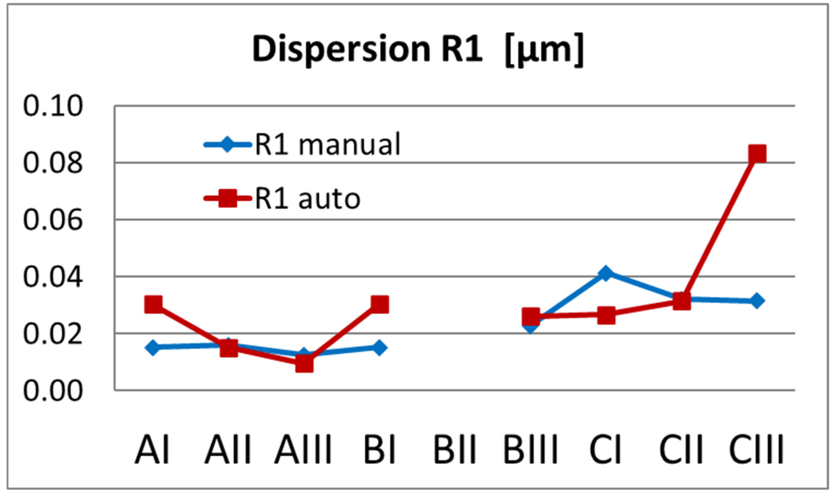
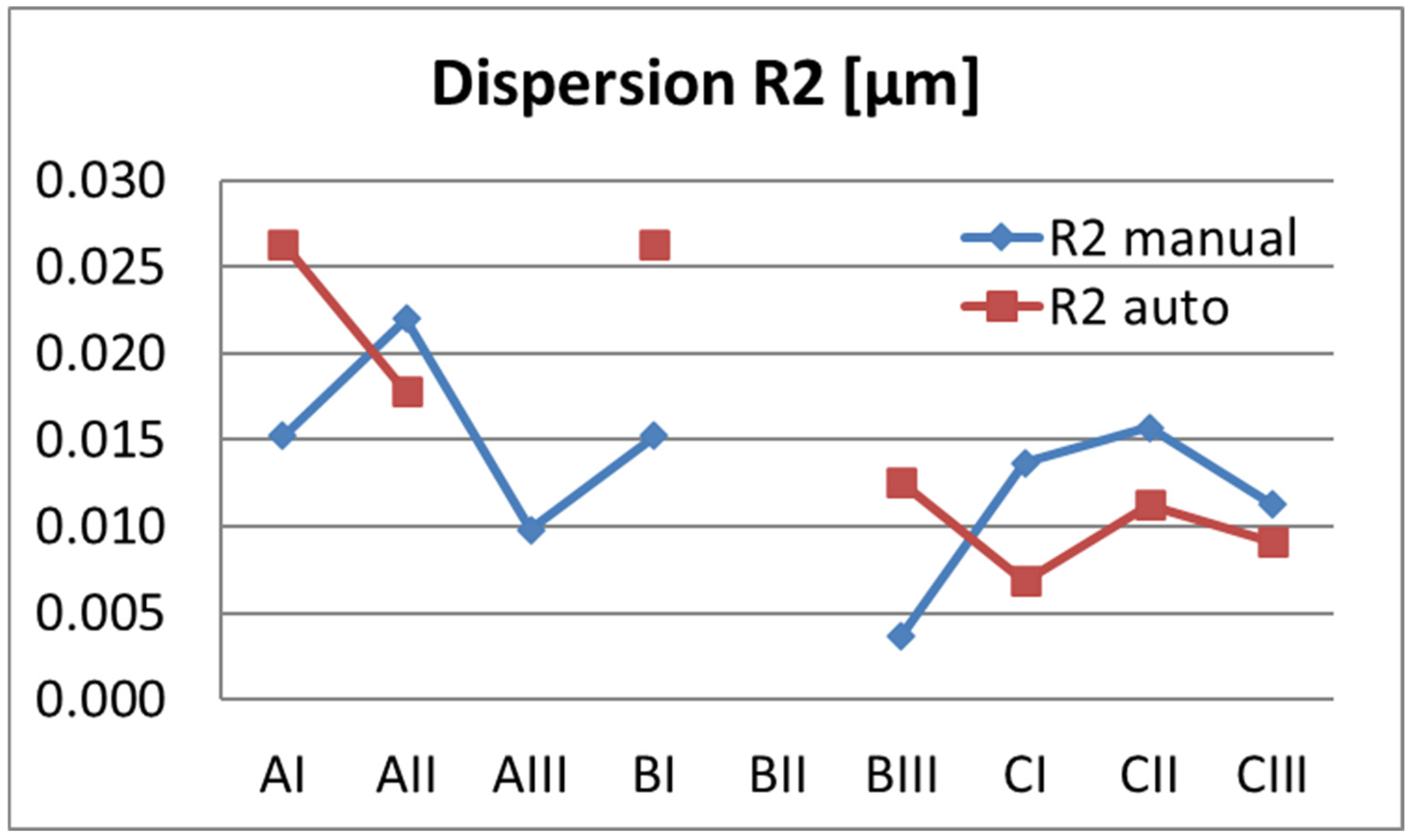
From Table 7 and Table 8, it follows that the maximum measurement uncertainty obtained for the Ri distances in the most recent calibration of the system was 15.5 µm. Consequently, by applying the 10% criterion commonly used in metrology, one arrives at the conclusion that a dispersion greater than 155 µm in the measurements may be indicative of an erroneous reading. By extension, it was decided that any Ri measurement presenting a dispersion greater than 1 mm would exceed this limit by a significant margin and, in the absence of any plausible cause other than a reading error, was discarded as spurious.

All the measurements developed are shown in the following figures (Figure 14, Figure 15, Figure 16 and Figure 17) for each distance.

The evolution of the R1 and R4 graphs from position BII onward is noteworthy (Figure 18, Figure 19, Figure 20 and Figure 21).

The same behavior occurs in both automatic and manual modes, suggesting a possible positioning error in the equipment.

The extremely high values of dispersion in R2 and R3 are due to spurious elements that affected the measurement results.

The variation in the Ri values falls within the expected measurement uncertainty and does not require any correction in the results. However, this procedure demonstrates how a simple test can provide valuable insight into the condition of the machine.

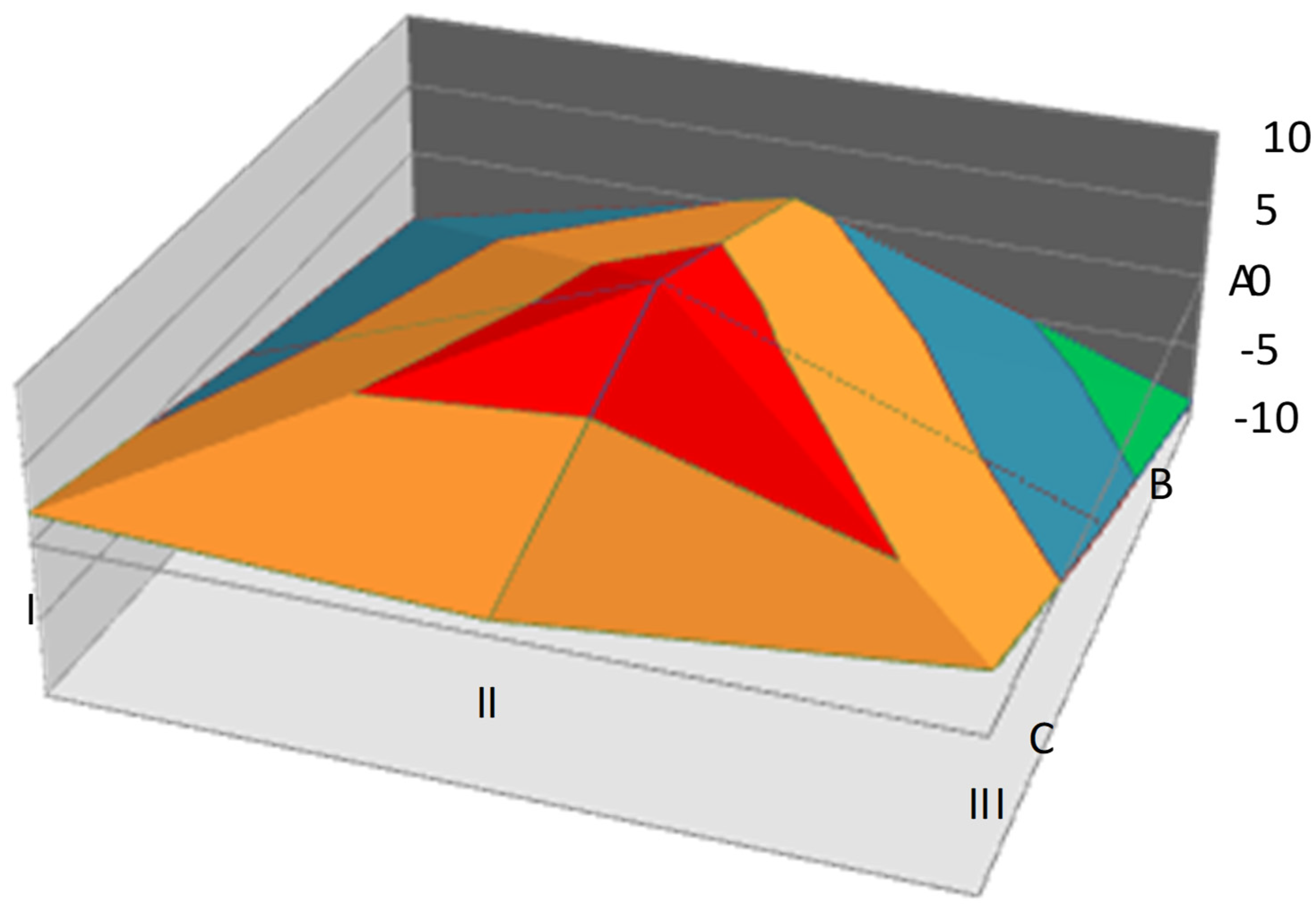
The results make it clear that the vision system exhibits a non-uniform metrological behavior across its measurement surface. The method reveals that the system does not behave homogeneously throughout the field of view: the dispersion of measurements varies significantly depending on the zone, with areas showing clearly superior repeatability and others presenting increased variability—even though the equipment is correctly calibrated (see Figure 22).

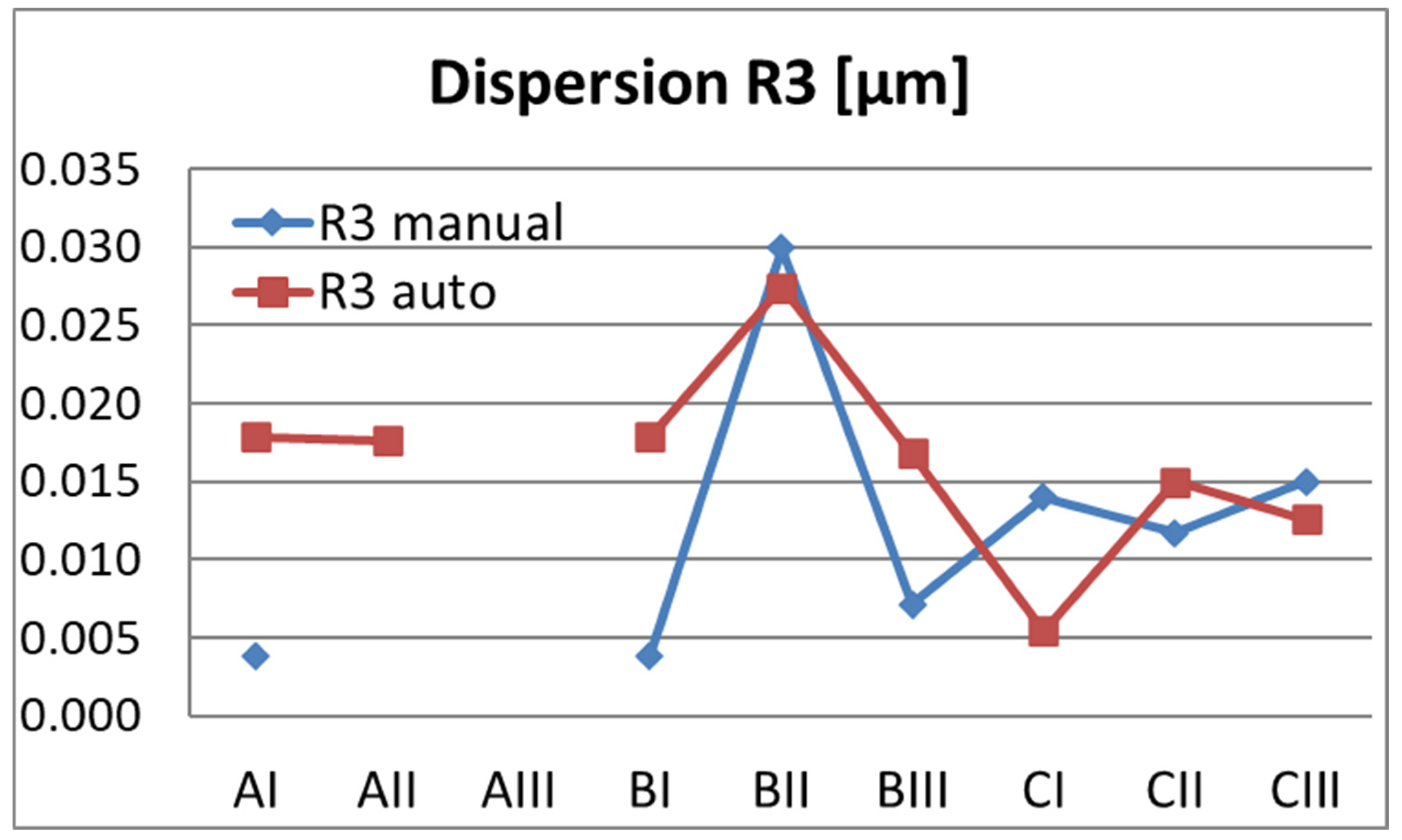
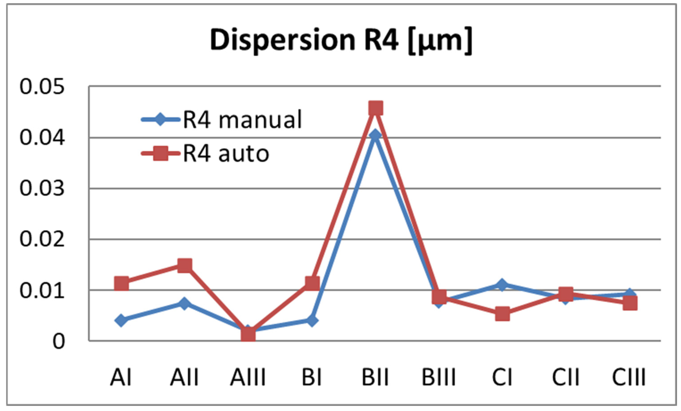
As shown in Figure 20, Figure 21 and Figure 22, the largest error and the poorest repeatability occur in the central region of the measurement table. Although this is particularly striking, it becomes understandable once the typical use of the equipment over time is examined. When such systems are first acquired, they generally exhibit minimal deviations in their central area, which leads users to routinely place the measurands there and to perform most measurements in that region. As time passes, this area undergoes the highest workload and consequently experiences greater wear, which may result in poorer repeatability and increased errors, as observed in this case. By contrast, the surrounding areas remain in comparatively good condition, meaning that placing the measurands elsewhere on the table is sufficient to continue achieving high-quality measurements. Thus, this method enables an ongoing assessment of the condition of the equipment across its entire measurement surface and supports an optimized use of the system. Several factors may contribute to this behavior, including localized mechanical wear, slight variations in focusing conditions, or positioning effects within the motion system.

This zonal characterization provides metrological information that cannot be obtained from a conventional, global calibration. By dividing the measurement surface into smaller regions, the method uncovers localized behaviors that remain hidden during standard verification procedures, enabling the identification of both optimal and degraded measurement areas.

The uncalibrated artifact used in the study shows sufficient dimensional stability for the purpose of interim verification, as consistent trends in both diameters and inter-sphere distances are maintained across all positions. The observed dispersion is therefore attributable to the measurement system, rather than to the artifact, supporting the use of such non-calibrated references for interim verification. Both the manual and automatic measurement modes reveal similar spatial trends; while the automatic mode reduces dispersion in some cases, it does not remove the zonal effects, confirming that these effects are intrinsic to the system, rather than linked to the operational mode. Importantly, although spatial variations are detected, they remain within the instrument’s calibration uncertainty, meaning that no premature recalibration is required—an aspect of practical relevance.

This approach also enables explicit identification of optimal and critical zones, allowing users to select regions of minimal dispersion for enhanced reliability, optimize part placement, and improve measurement performance without modifying the equipment. Finally, the robustness of the method is reinforced by its embedded outlier detection and acceptance/rejection criteria, which ensure that spurious values are discarded and that the characterization remains valid for real-world applications.

4. Discussion

Based on the diameter dispersion observed across the measurement volume, zones A and B exhibit the most reliable measurement performance.

Performing the measurements in both automatic and manual modes allows for verification of the result consistency.

From zone BII onward, an issue appears to affect the machine’s readings; however, the change is limited to R1 and R4. The remaining measurements are unaffected and therefore sufficient for verifying the system.

When operating in manual mode, high dispersion may occur, possibly due to less careful measurement. In such cases, the automatic mode proves to be more effective. Nevertheless, if measurements are taken with sufficient care, the manual mode tends to show less dispersion.

Following this procedure, a characterization of the vision system can be obtained. In the central area of the measurement volume, maximum dispersion values appear for some measurements, while no minimum dispersion values are observed. Contrary to initial expectations, the vision system shows the highest dispersion values in the center of the measurement area.

It can be concluded that the measurement area with the least dispersion corresponds to the lowest points in the surface graph shown above, while the highest points exhibit greater variability.

However, since all these values are below the calibration uncertainty of the equipment (0.6 µm), the calibration—and thus its traceability—does not need to be revised before the programmed time.

In some cases, zonal characterization may support the refinement of the overall measurement uncertainty model. However, this would involve additional work that the laboratory itself must evaluate.

In applications involving object recognition tasks, such as OCR, spatial variations in measurement performance may influence the recognition reliability, particularly when critical features are located in zones exhibiting higher dispersion.

The results clearly demonstrate that the proposed method reliably detects genuine metrological effects across the entire measurement surface while avoiding the introduction of artificial distortions or spurious artifacts. By leveraging a stable yet non-calibrated reference, the procedure reveals real variations in system behavior—such as local dispersion patterns or sensitivity to positioning—without compromising traceability or measurement integrity. Moreover, it provides meaningful metrological insights that traditional full-surface calibration does not typically uncover, particularly regarding spatial performance characterization, zone-dependent repeatability, and the identification of optimal measurement regions. These findings confirm that the method is both effective and highly informative for practical verification and long-term monitoring of vision-based measurement systems.

The proposed method has clear practical implications, as it enables informed decisions based on the spatial performance of the measurement surface. The identification of zones with lower dispersion supports the optimized positioning of measurands within the most stable regions of the field of view, thereby improving the measurement reliability without altering the calibration conditions. This capability provides a low-complexity and repeatable approach for improving the measurement performance within operational environments.

A key contribution of this work is the demonstration that the spatial behavior of the vision system is not intuitive. The observed increase in dispersion in central areas of the measurement surface challenges the common assumption that optical systems exhibit their best performance near the optical axis. Instead, the method reveals a complex spatial landscape in which the center does not necessarily correspond to the most stable zone. This insight underscores the importance of spatially resolved verification procedures and highlights limitations in conventional, globally applied calibration approaches that may mask these effects.

The method provides substantial practical advantages by offering meaningful metrological information with minimal setup, no need for costly calibrated artifacts, and short verification times. These characteristics make it particularly suitable for frequent interim verification procedures, where efficiency, continuity of operation, and low cost are essential. The approach can be easily incorporated into existing workflows, offering rapid and reproducible assessments of system performance without disrupting production.

Current challenges in optical metrology for manufacturing include the need for process-integrated vision systems, reduced verification times, decreased reliance on expensive calibrated standards, and continuous monitoring of system performance. The zonal, interim verification approach proposed in this work directly addresses these needs. It provides a flexible, cost-effective, and repeatable means of evaluating measurement-system behavior, contributing to the development of robust, automated, and production-ready optical metrology solutions. By addressing the practical limitations associated with conventional verification approaches, the method contributes to the integration of reliable, repeatable interim verification procedures within advanced manufacturing measurement systems. The results confirm that spatially resolved verification provides complementary information to global calibration procedures, without compromising traceability or normative compliance.

5. Conclusions

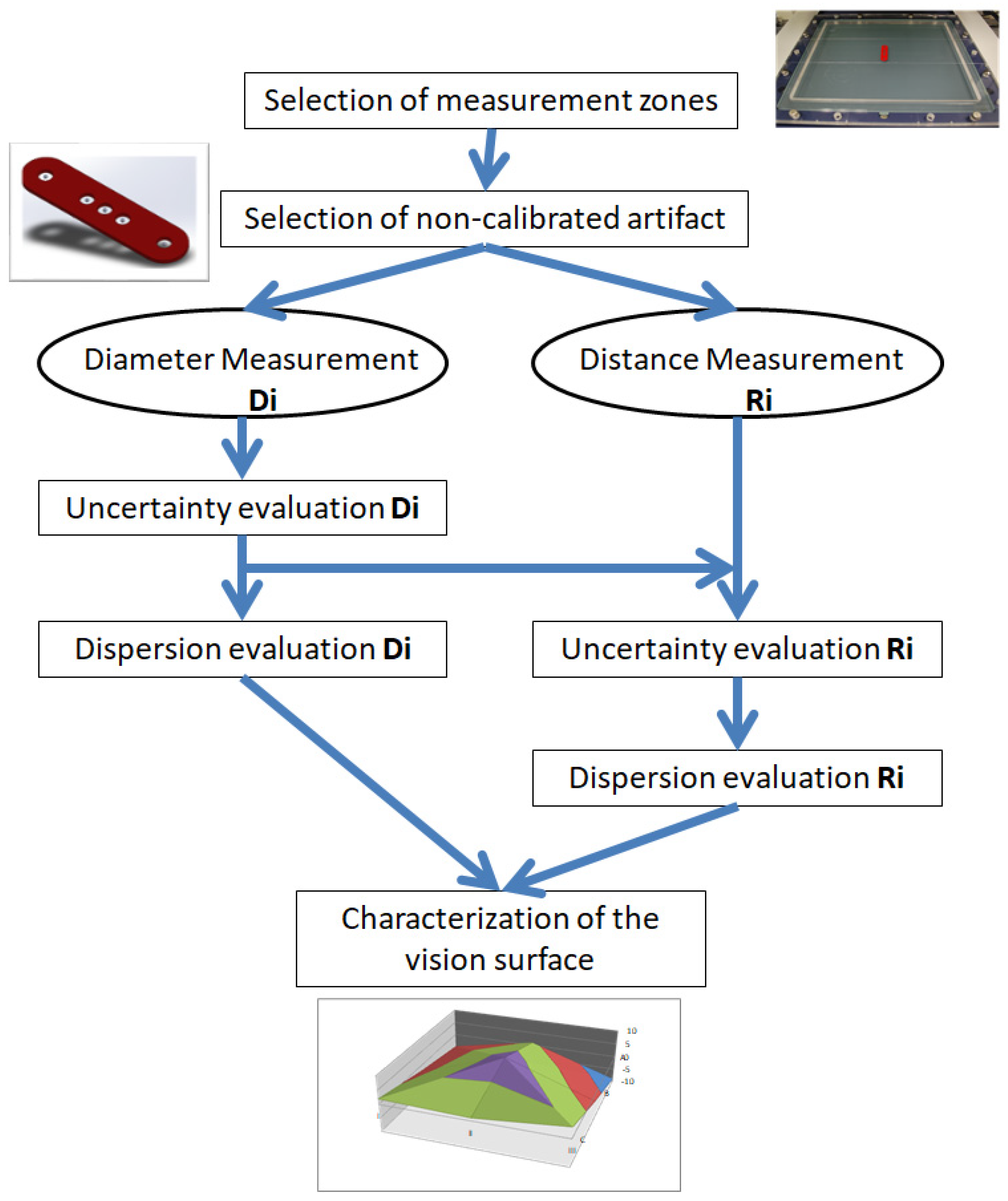
An important outcome of this study is the proposed procedure (see Figure 23) for the qualification and characterization of the measurement surface of the vision machine with an uncalibrated artifact:

• Division of the measurement surface into smaller areas for the characterization of each zone. For example, using an auxiliary device like the one shown in this study (Appendix B). The more exhaustive the meshing, the more information will be obtained about the measurement system, although it will also be more costly.
• Construction or acquisition of a non-calibrated artifact that includes at least two spheres and one distance for measurement. The conditions must be the same as those applied in the present study (Appendix A).
• Measurement of the diameters, Di, of the spheres in the artifact across all measurement zones of the system.
• Calculation of the uncertainty components, U_Di, of the sphere diameters, Di, in each measurement zone.
• Analysis of the dispersion of the diameters, Di, on the surface. This provides initial information about repeatability on the measurement surface.
• Measurement of the distances, Ri, between the spheres of the artifact in all measurement zones of the system.
• Calculation of the uncertainty components, U_Ri, of the distances, Ri, in each measurement zone.
• Analysis of the dispersion of the distances, Ri, on the surface. This provides complete information about the repeatability on the measurement surface.
• Characterization of the zones of the measurement surface where uncertainty and dispersion are minimal, thus identifying the optimal measurement area.
• As the dispersion of the radii of the spheres is kept well below the uncertainty of the equipment, the artifact is stable enough to perform this study in the equipment.

It is suggested that this study be conducted after equipment calibration on the scales, as well as an interim verification between calibrations, as suggested by standards for other measurement equipment.

The other main conclusions of this work may be summarized as:

• Methodological contribution: A zonal verification method for 2D vision-based measurement systems has been developed, using non-calibrated artifacts to assess the metrological behavior of the equipment between traceable calibrations. This approach provides a structured and repeatable framework for evaluating spatial performance across the measurement surface.
• Key findings: The study shows that the vision system exhibits significant spatial variability in measurement dispersion that cannot be detected through conventional global verification. The system does not behave uniformly over the entire field of view, and both optimal and degraded zones can be clearly identified, including counterintuitive effects such as increased dispersion in central regions.
• Practical value: Zonal characterization enables the explicit identification of optimal and critical measurement areas. This information can be directly applicable in measurement practice to improve measurement reliability by strategically positioning parts, without modifying the equipment or its calibration status.
• Metrological positioning: The proposed method does not replace traceable calibration; instead, it complements it as an effective interim verification tool. It provides additional metrological insight—unavailable through standard calibration procedures—while remaining fully aligned with normative and traceability principles.
• Broader applicability and projection: The approach is suitable for various optical metrology systems in manufacturing, including dimensional inspection and industrial vision-based measurement systems. Its low cost, speed, and suitability for frequent checks make it consistent with the demands of modern Industry 4.0 quality-control environments.

Figure 23. Proposed characterization procedure for Vision systems with an uncalibrated artifact.

Figure 23. Proposed characterization procedure for Vision systems with an uncalibrated artifact.

A promising line of future research involves integrating the proposed zonal verification procedure into automated self-monitoring routines within vision-based measurement systems. Embedding the method directly into the system’s control software would enable periodic interim verifications without operator intervention, supporting continuous health monitoring of the measurement surface and enabling early detection of performance drifts. Such automated routines could contribute to more robust, autonomous quality-assurance strategies and align with the broader objective of developing self-calibrating or self-verifying optical systems that are suitable for high-throughput industrial environments.

Another important direction is the evaluation of the method in real production settings, where factors such as lighting fluctuations, ambient vibration, thermal variation, and dynamic machine operation can affect measurement repeatability. Testing the approach under these real-world conditions would provide insight into its robustness and practical utility for in-line verification, especially in demanding manufacturing processes. This would not only validate the method beyond controlled laboratory scenarios but also help to refine it for deployment in industrial vision systems, including OCR-based inspection, dimensional control, and process-integrated optical metrology.

The material employed for the artifact must exhibit long-term stability so that it neither deforms nor degrades under working conditions. Metal spheres were selected because they represent geometrically robust shapes for determining center-to-center distances, a measurement that is only minimally influenced by minor surface imperfections. The same criteria apply to the structure designed to hold the spheres in place. Other materials could also be used, provided that they maintain dimensional stability and that their spherical geometry can be reliably ensured.

The use of a non-calibrated artifact enables more frequent verification of the equipment, as such artifacts do not require calibration and therefore allow for sufficiently reliable checks to conduct a detailed monitoring of the system’s performance. Although this approach does not replace the periodic calibrations that must be carried out for each axis of the equipment, it does provide assurance of proper functioning between calibrations. Moreover, should any issue or deviation arise, it allows for its rapid detection, rather than remaining unnoticed until the next scheduled calibration—thus preventing potential measurement errors that could otherwise occur while using a misaligned system.

Although this work is oriented toward the verification of a 2D vision system that is typically used in metrology, it lays the foundations for the verification of OCR systems. Once the method has been demonstrated to be valid for the verification of equipment providing calibration services in industry, the research group is currently working on implementing this approach for OCR-dedicated systems, enabling rapid verification. In this way, the automation of historical texts with complex handwriting will be significantly streamlined.

The proposed method therefore complements conventional calibration procedures by providing a practical tool for the interim verification and spatial performance monitoring of vision-based measurement systems.

References

- Nanna, N.; Chanthawong, N.; Buajarern, J. Design and development of OCR software for remote measurement and calibration. J. Phys. Conf. Ser. 2023, 2653, 012012. [Google Scholar] [CrossRef]
- Slossberg, R.; Anschel, O.; Markovitz, A.; Litman, R.; Aberdam, A.; Tsiper, S.; Mazor, S.; Wu, S.; Manmatha, R. On calibration of scene-text recognition models. In European Conference on Computer Vision; Springer Nature Switzerland: Cham, Switzerland, 2022; pp. 263–279. [Google Scholar]
- Hamad, K.; Kaya, M. A detailed analysis of optical character recognition technology. Int. J. Appl. Math. Electron. Comput. 2016, 4, 244–249. [Google Scholar] [CrossRef]
- Allen, M. Optical character recognition: Technology with new relevance for archival automation projects. Am. Arch. 1987, 50, 88–99. [Google Scholar]
- Sahu, N.; Sonkusare, M. A study on optical character recognition techniques. Int. J. Comput. Sci. Inf. Technol. Control Eng. 2017, 4, 1–15. [Google Scholar] [CrossRef]
- Stoliński, S.; Bieniecki, W. Application of OCR systems to processing and digitization of paper documents. Inf. Syst. Manag. VII 2011, 102, 1–9. [Google Scholar]
- Sinha, R. Digitization of Document and Information Extraction using OCR. arXiv 2025, arXiv:2506.11156. [Google Scholar] [CrossRef]
- Monteiro, G.; Camelo, L.; Aquino, G.; Fernandes, R.D.A.; Gomes, R.; Printes, A.; Figueiredo, C. A comprehensive framework for industrial sticker information recognition using advanced OCR and object detection techniques. Appl. Sci. 2023, 13, 7320. [Google Scholar] [CrossRef]
- Subedi, B.; Yunusov, J.; Gaybulayev, A.; Kim, T.H. Development of a low-cost industrial OCR system with an end-to-end deep learning technology. IEMEK J. Embed. Syst. Appl. 2020, 15, 51–60. [Google Scholar] [CrossRef]
- Čakić, S.; Popović, T.; Šandi, S.; Krčo, S.; Gazivoda, A. The use of tesseract OCR number recognition for food tracking and tracing. In 2020 24th International Conference on Information Technology (IT); IEEE: Piscataway, NJ, USA, 2020; pp. 1–4. [Google Scholar] [CrossRef]
- Singh, A.; Bacchuwar, K.; Bhasin, A. A survey of OCR applications. Int. J. Mach. Learn. Comput. 2012, 2, 314–318. [Google Scholar] [CrossRef]
- Chaiyapet, P.; Wattana, B. Development of Tracking and Backward Tracing System for an Automotive Parts Using Optical Character Recognition Technique. In Proceedings of the 2024 9th International STEM Education Conference (iSTEM-Ed); IEEE: Piscataway, NJ, USA, 2024; pp. 1–4. [Google Scholar] [CrossRef]
- Peng, X.; Cao, H.; Setlur, S.; Govindaraju, V.; Natarajan, P. Multilingual OCR research and applications: An overview. In Proceedings of the 4th International Workshop on Multilingual OCR, Washington, DC, USA, 24 August 2013; pp. 1–8. [Google Scholar]
- Banoth, R.; Arunakranthi, G.; Vachhani, P.; Kalaria, S.; Rathod, R. Implementation and mitigation for cyber attacks with proposed OCR process model. Nat. Volatiles Essent. Oils 2021, 8, 2149–2160. [Google Scholar]
- Qi, S.; Sun, Q.; Cheng, C.; Wang, Z.; Gao, Z.; Liu, J. Design of Document Secret Level Consistency Check Software Based on OCR. In Proceedings of the 2024 7th International Conference on Computer Information Science and Application Technology (CISAT); IEEE: Piscataway, NJ, USA, 2024; pp. 614–618. [Google Scholar] [CrossRef]
- Yimyam, W.; Ketcham, M.; Jensuttiwetchakult, T.; Hiranchan, S.; Pramkeaw, P.; Chumuang, N. Enhancing and Evaluating an Impact of OCR and Ontology on Financial Document Checking Process. In Proceedings of the 2020 15th International Joint Symposium on Artificial Intelligence and Natural Language Processing (iSAI-NLP); IEEE: Piscataway, NJ, USA, 2020; pp. 1–6. [Google Scholar] [CrossRef]
- JCGM. International Vocabulary of Metrology—Basic and General Concepts and Associated Terms (VIM) (JCGM 200:2008); Bureau International des Poids et Mesures (BIPM): Sèvres, France, 2008; Available online: https://www.cem.es/es/divulgacion/documentos/vocabulario-internacional-metrologia-vim-3a-edicion-2012-espanol (accessed on 15 February 2026).
- Centro Español de Metrología. Clasificación de instrumentos de metrología dimensional. In Clasificación de Instrumentos de Metrología Dimensional, 1st ed.; Ministerio de Fomento, Ed.; Ministerio de Fomento: Madrid, Spain, 2002. [Google Scholar]
- Mitutoyo GmbH. Instrumentos de medida de precisión. In Catálogo Instrumentos de Medida de Precisión E-4001, 1st ed.; Mitutoyo GmbH, Ed.; Mitutoyo GmbH: Neuss, Germany, 1991. [Google Scholar]
- UNE-EN ISO 10360-2:2010; Geometrical Product Specifications (GPS). Acceptance and Reverification Tests for Coordinate Measuring Machines (CMM). Part 2: CMMs Used for Measuring Linear Dimensions. AENOR: Madrid, Spain, 2010.
- UNE-EN ISO 15530-3:2011; Geometrical Product Specifications (GPS). Coordinate Measuring Machines (CMM): Technique for Determining the Uncertainty of Measurement. Part 3: Use of Calibrated Workpieces or Measurement Standards. AENOR: Madrid, Spain, 2011.
- FREMAP. Dimensional Metrology Laboratory Accredited by ENAC. Calibration Process PF-013 for Vernier Calipers D-02.02, 14th ed.; FREMAP: Madrid, Spain, 2010. [Google Scholar]
- JCGM/WG 1. Guide to the Expression of Uncertainty in Measurement—Part 1: Introduction, 1st ed.; Joint Committee for Guides in Metrology, Ed.; BIPM: Sèvres, France, 2023; pp. 1–54. Available online: https://www.bipm.org/documents/20126/2071204/JCGM_GUM-1.pdf (accessed on 15 February 2026).
Figure 1.
Thermohygrograph.
Figure 2.
Quick Vision ELF vision machine.
Figure 3.
Uncalibrated artifact.
Figure 4.
Uncalibrated artifact technical drawing. Distance between spheres. From left to right: spheres D1, D2, D3, D4, and D5.
Figure 5.
Physical artifact to be measured, with markings to indicate the measurement direction.
Figure 6.
Methacrylate support delimiting the measurement zones. Uncalibrated artifact in the center.
Figure 7.
Artifact and methacrylate support during measurement.
Figure 8.
Identification of measurement zones.
Figure 9.
Measurement zones and nomenclature defined from the spatial arrangement of the spheres. Horizontal lines indicate the reference positions, arrows represent the measurement direction, and numbered boxes identify the different measurement regions considered in the analysis.
Figure 10.
Diameter measurements of each sphere at each position on the table (manual mode).
Figure 11.
Diameter measurements of each sphere at each position on the table (auto mode).
Figure 12.
Diameter dispersion of each sphere at each table position (manual mode).
Figure 13.
Diameter dispersion of each sphere at each table position (auto mode).
Figure 14.
Evolution of the R1 distance measurements (manual and auto mode).
Figure 15.
Evolution of the R2 distance measurements (manual and auto mode).
Figure 16.
Evolution of the R3 distance measurements (manual and auto mode).
Figure 17.
Evolution of the R4 distance measurements (manual and auto mode).
Figure 18.
Evolution of the dispersions in the R1 distance measurements (manual and auto mode).
Figure 19.
Evolution of the dispersions in the R2 distance measurements (manual and auto mode).
Figure 20.
Evolution of the dispersions in the R3 distance measurements (manual and auto mode).
Figure 21.
Evolution of the dispersions in the R4 distance measurements (manual and auto mode).
Figure 22.
Representation of the measurement zones and their corresponding deviations. Colors indicate the magnitude of deviation, with red representing the highest values, orange and yellow intermediate values, and blue/green the lowest values. The letters (A–C) denote the positions along one axis, while the Roman numerals (I–III) indicate the positions along the perpendicular axis, defining the spatial distribution of the measurement regions.