Neuro-Adaptive Control for a Balance Board: Comparative Study with PID and LQR

Abstract

Balance is an essential component in both everyday movement and sports performance. Balance boards are commonly used for training and physical therapy to improve balance. Conventional balance boards primarily rely on the user’s voluntary actions, whereas active/actuated balance boards can provide dynamic motion for both balance and rehabilitation. While this enables more effective training, it also introduces strong user-dependent and time-varying dynamics that are difficult to regulate with conventional controllers. This study addresses this limitation by developing a neuro-adaptive sliding mode controller to handle the strong inter-user variability and nonlinear pressure–force dynamics of pneumatic artificial muscles. The controller combines a learning neural network that updates online with a robust control structure to ensure stable motion in the presence of disturbances. The proposed approach was evaluated against commonly used PID and LQR controllers under sudden changes in operating conditions. Simulation results show that the proposed controller improves stability, reduces control effort, and adapts more effectively to different users and external disturbances. These findings suggest that neuro-adaptive control strategies can improve the reliability and responsiveness of balance training and rehabilitation devices, supporting safer and more personalized therapy.

1. Introduction

Balance and motor control are fundamental to the safe performance of daily tasks. These abilities are closely associated with functional outcomes in both athletic and rehabilitation settings [1,2]. Impairments in postural stability and coordination have been associated with an increased risk of injuries and falls, particularly among older adults and athletes [1,3]. Therefore, balance exercises are widely incorporated into clinical rehabilitation programs and sport-specific training protocols to improve dynamic postural control. These protocols include destabilizing conditions for more adaptive training procedures [4].

Balance boards are widely used in rehabilitation and sports science for balance exercises [5]. These tools promote continuous postural adjustments and increased neuromuscular activation by creating controlled instability. These features make them effective in developing dynamic stability [6]. Traditional passive balance boards rely almost entirely on the user’s reflexes. They do not account for individual differences or progress over time. Active and robotic systems overcome this limitation by generating controlled movements that either assist or challenge the user. Thus, they provide a much more personalized training experience [7].

Active balance boards are structurally nonlinear and underactuated systems [8]. Since these applications involve direct human–system interaction, factors such as user behavior, environmental noise, and time-varying uncertainties continually alter the system dynamics. This situation makes it difficult to achieve fast and precise balance control and often pushes the limits of classical control methods [9]. Managing this variability requires control strategies that can respond quickly without compromising safety or stability.

Common control strategies for balance systems include Proportional-Integral-Derivative (PID) controllers, Linear Quadratic Regulators (LQR), and classical adaptive methods [7,10]. Although these methods are favored for their simplicity and theoretical maturity, they often fall short when faced with nonlinear or uncertain dynamics. For example, PID controllers require extensive tuning and exhibit poor robustness to uncertainty, whereas LQR-based approaches lose effectiveness under changing conditions due to their reliance on precise mathematical models [11,12].

Similarly, classical adaptive techniques often rely on rigid uncertainty models and may struggle to respond quickly to the rapid, complex dynamics observed in human-in-the-loop systems, time-varying uncertainties, and human interaction issues in isolation rather than within a unified framework [9,13]. The system must adapt to individual user needs simultaneously [14,15].

This study presents a neuro-adaptive sliding-mode control strategy for real-time balance control of a balance board actuated by pneumatic artificial muscles. By combining the inherent robustness of sliding mode control with the online learning capability of neural networks. This approach effectively compensates for nonlinearities and system uncertainties [16,17,18]. Rather than relying on a precise prior model, the neuro-adaptive framework identifies unknown dynamics in real time, thereby improving balance precision while preserving closed-loop stability [19,20].

This work validates a neuro-adaptive sliding mode controller for a pneumatically actuated balance board through mathematical modeling and simulation. In evaluations conducted against standard PID and LQR benchmarks, the proposed strategy consistently demonstrated superior stability and reduced control effort, even under sudden disturbances or varying user profiles. In conclusion, the obtained findings provide a reference for the future development of adaptive control in rehabilitation robotics and human–machine interaction.

2. Materials and Methods

Pneumatic artificial muscles (PAMs) are soft actuators consisting of a flexible membrane enclosed in a braided shell, which generate unidirectional linear pulling force through axial contraction and radial expansion under compressed air, making them well-suited for robotic and assistive applications [7,21].

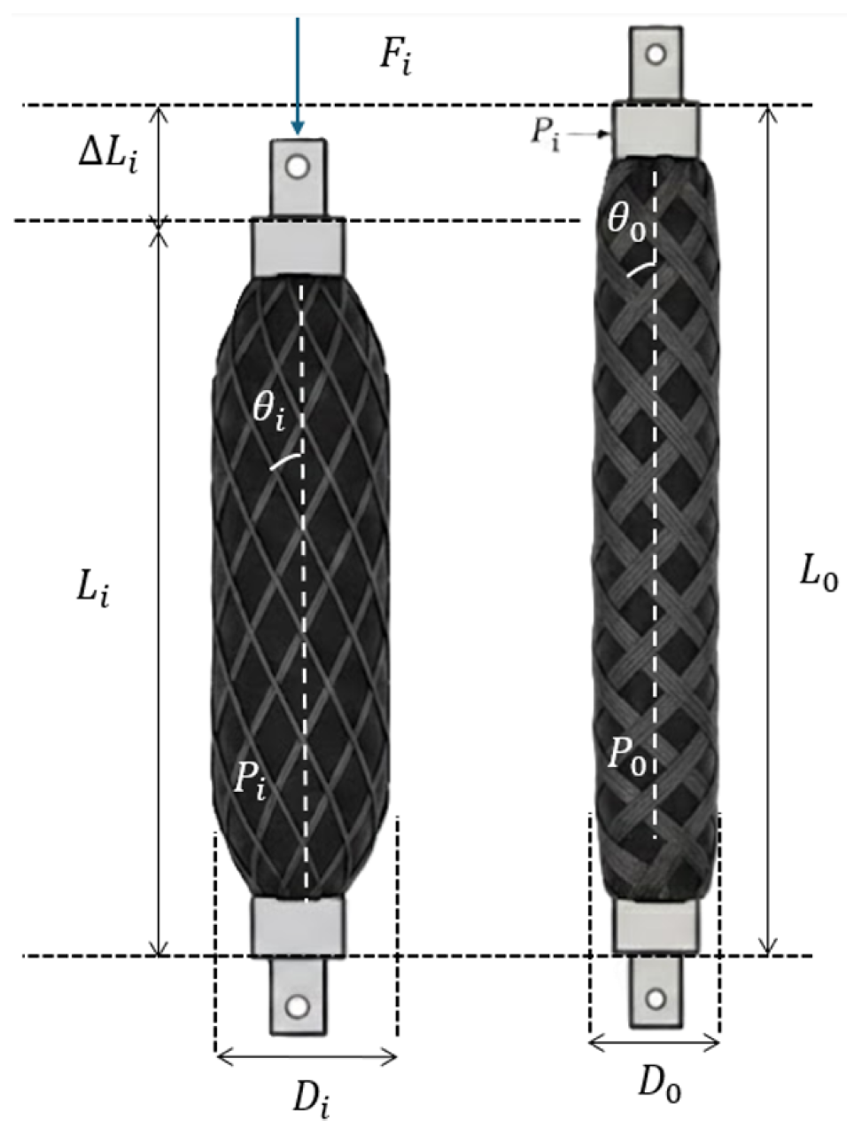
McKibben PAMs operate under the principle of interaction between internal pressure and structural deformation [22,23]. As seen in Figure 1, the PAM is made of a cylindrical membrane covered with braided fibers. Under an internal pressure P, the membrane undergoes radial expansion $(D_i>D_0)$ while simultaneously contracting in the axial direction $(L_i<L_0)$. This deformation is geometrically related to the initial and final braid angles, ${\theta }_0$ and ${\theta }_i$, respectively, which directly influence the generated actuation forces [24,25,26]. Based on the principle of conservation of energy, the force exerted by PAM can be modeled to lead to the fundamental equation.

Using the Chou–Hannaford model [22], the pulling force of a PAM under internal pressure can be expressed as follows:

$$F=P{\displaystyle \frac{\pi D_0^2}{4}}{\displaystyle \frac{b^2-L^2}{b^2-D_0^2}},$$

(1)

where F denotes the pulling force, P is the internal gauge pressure, L is the muscle length, $D_0$ is the nominal diameter at rest, and b represents the length of the braided fibers.

This model describes the tensile force at the ends of the muscle as a function of internal pressure and the system’s geometric parameters. It is commonly used to analyze the behavior of the PAM under external load.

When the muscle ends are completely free to contract, the net axial force F can be considered zero. In this case, the numerator term $(b^2-L^2)$ in (1) approaches zero, implying that the muscle length L decreases to a value dictated by the braid geometry. Experimentally, or when additional geometric constraints are taken into account, the muscle length is observed to reach a minimum contraction length, denoted as $L_{min}$. 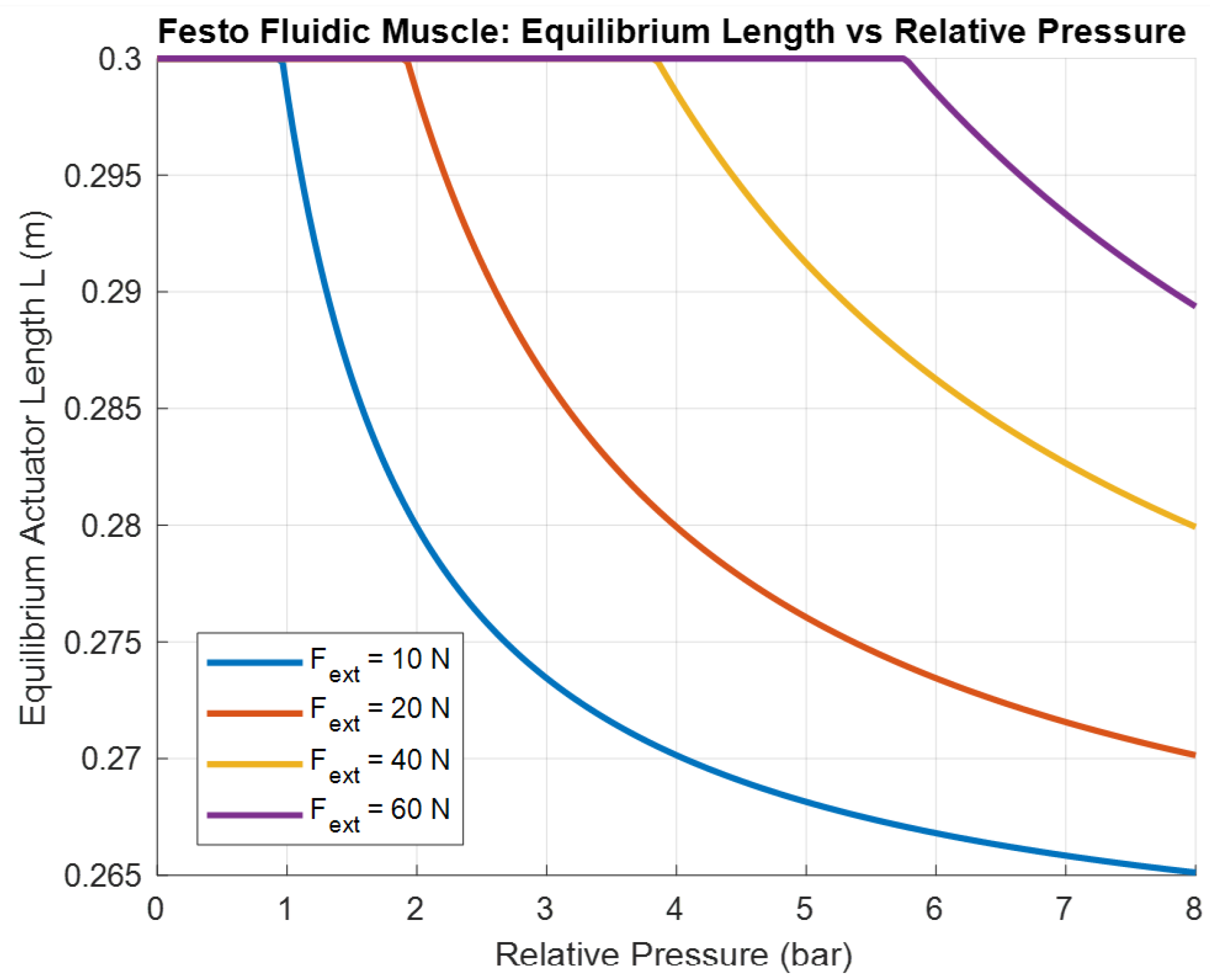As illustrated in Figure 2, the PAM length varies with internal pressure, decreasing from a maximum length of approximately 0.3 m to a minimum length of approximately 0.26 m while different trajectories vary external forces.

Practical pneumatic systems exhibit additional dynamics due to air compressibility, valve flow limitations, and chamber volume effects. These phenomena introduce a delay between the commanded pressure and the effective pressure within the muscle chamber.

To incorporate this effect, a first-order lag model was introduced in the pressure dynamics. The effective internal pressure of each PAM, $P_{\mathrm{eff}}\left(t\right)$, was modeled as

$${\tau }_p{\dot{P}}_{\mathrm{eff}}\left(t\right)+P_{\mathrm{eff}}\left(t\right)=P_{\mathrm{cmd}}\left(t\right),$$

(2)

where $P_{\mathrm{cmd}}\left(t\right)$ denotes the commanded pressure signal generated by the controller and ${\tau }_p$ represents the pneumatic time constant associated with compressibility and valve dynamics. In the simulations, the lag time constant was set to ${\tau }_p=0.02\mathrm{s}$.

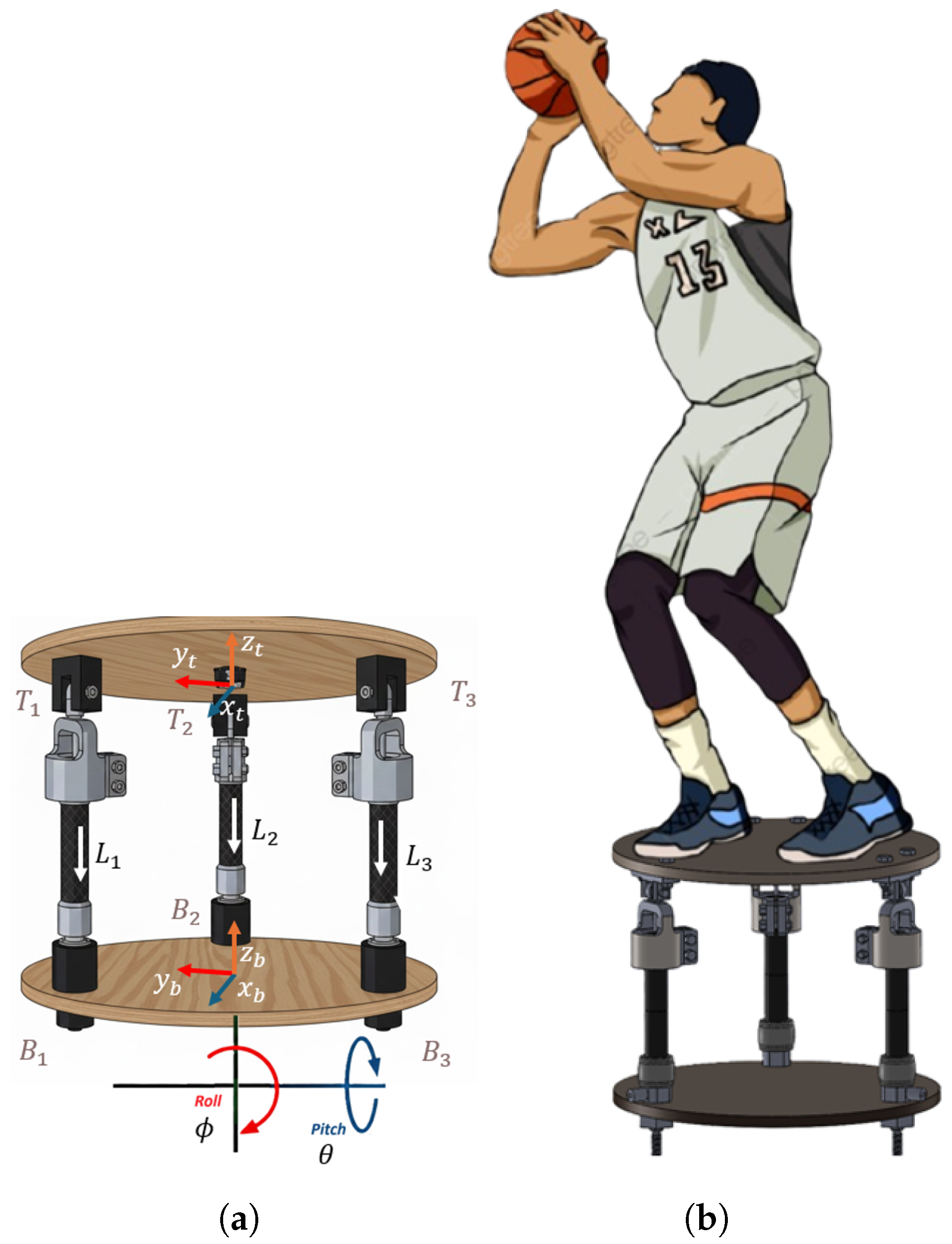
Figure 3a is the structure of the PAM-actuated balance board. The active balance board (ABB) analyzed in this paper consists of three PAMs connected at the apexes of an equilateral triangle, forming the base and the moving platform [27].

For the kinematic description of the system, the generalized coordinate vector is defined as $\mathbf{q}={[\varphi ,\theta ]}^T$, where $\varphi$ and $\theta$ denote the Euler angles corresponding to rotations about the x-axis (roll) and the y-axis (pitch), respectively. The configuration $\varphi =0$, $\theta =0$ represents the nominal flat state of the platform. Each muscle i is connected between a fixed attachment point ${\mathbf{B}}_i$ on the base platform and a moving attachment point ${\mathbf{T}}_i(\varphi ,\theta )$ on the moving platform.

The base attachment points ${\mathbf{B}}_1,{\mathbf{B}}_2,{\mathbf{B}}_3\in {\mathbb{R}}^3$ denote the three-dimensional coordinates of the muscle endpoints on the base platform. The position of the moving platform is described using the transformation given in Equation (3), with an additional small constant offset vector ${\mathbf{p}}_0$ to account for geometric misalignment or assembly tolerances.

$${\mathbf{T}}_i(\varphi ,\theta )=\mathbf{R}(\varphi ,\theta ){\mathbf{T}}_i^0+{\mathbf{p}}_0$$

(3)

Here, $\mathbf{R}(\varphi ,\theta )$ is the rotation matrix corresponding to the pitch and roll angles (e.g., using Z-Y-X or some Euler-angle convention). Hence, each muscle length $L_i(\varphi ,\theta )$ is the Euclidean distance between ${\mathbf{B}}_i$ and ${\mathbf{T}}_i(\varphi ,\theta )$.

$$L_i(\varphi ,\theta )=\parallel {\mathbf{T}}_i(\varphi ,\theta )-{\mathbf{B}}_i\parallel$$

(4)

Because of ${\mathbf{T}}_i(\varphi ,\theta )$, the generally contained trigonometric functions dependence of $\varphi ,\theta$, $L_i$ also becomes a trigonometric, highly nonlinear function in those angles. A simplified rigid-body approach is shown in Equation (5).

$$\mathbf{M}\left(\mathbf{q}\right)\ddot{\mathbf{q}}+\mathbf{C}(\mathbf{q},\dot{\mathbf{q}})\dot{\mathbf{q}}+\mathbf{g}\left(\mathbf{q}\right)={\mathbf{\tau }}_{\mathrm{PAM}}\left(\mathbf{u}\right)+{\mathbf{d}}_{\mathrm{ext}}$$

(5)

where $\mathbf{M}\left(\mathbf{q}\right)$ is the inertia/mass matrix, $\mathbf{C}(\mathbf{q},\dot{\mathbf{q}})$ the Coriolis/centrifugal coupling, $\mathbf{g}\left(\mathbf{q}\right)$ the gravity term, ${\mathbf{\tau }}_{\mathrm{PAM}}\left(\mathbf{u}\right)$ and the net torque produced by the three PAMs as a function of the input pressure $\mathbf{u}$. ${\mathbf{d}}_{\mathrm{ext}}$ is external disturbance.

We define $\mathbf{u}=[u_1,u_2,u_3]$ as the pressure control inputs to each muscle. Each muscle’s force depends on u pressure and the muscle’s length $L_i(\varphi ,\theta )$. Summing the three muscle forces about the board’s pivot yields ${\tau }_{\varphi }$ (pitch torque) and ${\tau }_{\theta }$ (roll torque).

$$\left[\begin{array}{c}{\tau }_{\varphi }\\ {\tau }_{\theta }\end{array}\right]=f(\varphi ,\theta ,u_1,u_2,u_3)$$

(6)

Here, $f(·)$ is nonlinear due to the geometry and the Chou–Hannaford muscle force expression. Due to the inherent uncertainties and time-varying characteristics of PAM systems, accurate modeling is challenging. Thus, nominal parameters and their mismatch errors are introduced explicitly. PAM torque (${\mathbf{\tau }}_{\mathrm{PAM}}$) generated by the three PAMs is described clearly by Chou–Hannaford’s model as a function of the pressure input $\mathbf{u}$,

$${\mathbf{\tau }}_{\mathrm{PAM}}\left(\mathbf{u}\right)=\mathbf{J}{\left(\mathbf{q}\right)}^T{\mathbf{F}}_{\mathrm{PAM}}\left(\mathbf{u}\right)$$

(7)

Here, $\mathbf{J}{\left(\mathbf{q}\right)}^T$ is the Jacobian mapping of PAM forces to Euler angle torques, defined by platform geometry. ${\mathbf{F}}_{\mathrm{PAM}}\left(\mathbf{u}\right)$ are the PAM-generated forces, defined as per Chou–Hannaford as given in the Equation (8).

$${\mathbf{F}}_{\mathrm{PAM}}\left(u\right)={\displaystyle \frac{\pi D_0^{2}u}{4}}\left[3{\left({\displaystyle \frac{L_0}{L}}\right)}^2-1\right]$$

(8)

Here, the PAM torque ${\mathbf{\tau }}_{\mathrm{PAM}}$ is explicitly linear in the pressure input u. We can rewrite clearly as,

$${\mathbf{\tau }}_{\mathrm{PAM}}\left(\mathbf{u}\right)=\mathbf{A}(\mathbf{q},\mathbf{L})\mathbf{u}$$

(9)

Here, $\mathbf{A}(\mathbf{q},\mathbf{L})$ is known geometry and length-dependent terms with $\mathbf{A}(\mathbf{q},\mathbf{L})=\mathbf{J}{\left(\mathbf{q}\right)}^T{\displaystyle \frac{\pi D_0^2}{4}}\left[3{\left({\displaystyle \frac{L_0}{L}}\right)}^2-1\right]$. This term is explicitly computable from geometry and instantaneous muscle lengths.

The explicit acceleration equation is thus derived by rearranging the original dynamics equation as follows:

$$\ddot{\mathbf{q}}=\mathbf{M}{\left(\mathbf{q}\right)}^{-1}\left[-\mathbf{C}(\mathbf{q},\dot{\mathbf{q}})\dot{\mathbf{q}}-\mathbf{g}\left(\mathbf{q}\right)+{\mathbf{d}}_{\mathrm{ext}}\right]+\mathbf{M}{\left(\mathbf{q}\right)}^{-1}\mathbf{A}(\mathbf{q},\mathbf{L})\mathbf{u}$$

(10)

In practical scenarios, uncertainties in mechanical parameters and actuator dynamics, as well as external disturbances, significantly affect system performance. Therefore, robust control strategies are essential to guarantee accurate and stable system operation. If we rewrite the system dynamics.

$$\ddot{\mathbf{q}}=\mathbf{F}(\mathbf{q},\dot{\mathbf{q}},\mathbf{u})+\mathbf{M}{\left(\mathbf{q}\right)}^{-1}\mathbf{A}(\mathbf{q},\mathbf{L})\mathbf{u}$$

(11)

Here, $\mathbf{F}(\mathbf{q},\dot{\mathbf{q}},\mathbf{u})$ is an unknown nonlinear function, giving us a vector equation in the form as shown in Equation (12).

$$\mathbf{F}(\mathbf{q},\dot{\mathbf{q}},\mathbf{u})=\mathbf{M}{\left(\mathbf{q}\right)}^{-1}\left[-\mathbf{C}(\mathbf{q},\dot{\mathbf{q}})\dot{\mathbf{q}}-\mathbf{g}\left(\mathbf{q}\right)+{\mathbf{d}}_{\mathrm{ext}}\right]$$

(12)

This $\mathbf{F}(·)$ is what we will approximate with a multi-layer neural network in real time. A 3-layer network with weights ${\mathbf{W}}_i$ (input layer) and ${\mathbf{W}}_o$ (output layer) approximates $\hat{\mathbf{F}}(·)$:

$$\hat{\mathbf{F}}(·)\approx {\mathbf{W}}_o^{\top }\sigma \left({\mathbf{W}}_i^{\top }\mathbf{X}\right)$$

(13)

Here, $\mathbf{X}={[\varphi ,\theta ,\dot{\varphi },\dot{\theta },u_1,u_2,u_3,1]}^{\top }$, is the neural network input vector, including a constant 1 for bias, $\sigma (·)$ is a sigmoid activation function of neurons in the hidden layer.

$$\mathbf{z}={\mathbf{W}}_i^{\top }\mathbf{X},\sigma \left(\mathbf{z}\right)={\displaystyle \frac{1}{1+e^{-\mathbf{z}}}}$$

(14)

Here, ${\mathbf{W}}_i$ is the input weight matrix in the dimension of input (in this case $1\times 8$), and $\sigma \left(\mathbf{z}\right)$ is the elementwise sigmoid function output of the layer. $\sigma \left(\mathbf{z}\right)$ and its derivative $\dot{\sigma }\left(\mathbf{z}\right)$ are both bound. The output layer is

$$\hat{\mathbf{F}}={\mathbf{W}}_o^{\top }\sigma \left(\mathbf{z}\right)=\left[{\hat{F}}_{\varphi },{\hat{F}}_{\theta }\right]$$

(15)

Here, ${\mathbf{W}}_o$ is an output layer weight matrix in the dimension of hidden layer times output (since we need 2 outputs, $\ddot{\varphi }$ and $\ddot{\theta }$, it can be described as ${\mathbf{W}}_o\in {\mathbb{R}}^{n_h\times 2}={\mathbb{R}}^{HLS\times 2}$) The proposed neural network contains a single hidden layer with $n_h=10$ neurons.

2.1. Control Strategy

For the control of the system for desired Euler angles like ${\mathbf{q}}_d={[{\varphi }_d,{\theta }_d]}^T$. We can define controller errors as shown in Equation (16).

$$\mathbf{e}\left(t\right)\triangleq \mathbf{q}\left(t\right)-{\mathbf{q}}_d\left(t\right),\dot{\mathbf{e}}\left(t\right)\triangleq \dot{\mathbf{q}}\left(t\right)-{\dot{\mathbf{q}}}_d\left(t\right),\mathbf{e}=[e_{\varphi },e_{\theta }]$$

(16)

For robust control of the system, we define a sliding surface $\mathbf{s}\left(t\right)$ that dictates the desired dynamics in the error domain, as depicted in the following equation.

$$\mathbf{s}\left(t\right)=\mathbf{\Lambda }\mathbf{e}\left(t\right)+\dot{\mathbf{e}}\left(t\right),\mathbf{\Lambda }=\mathrm{diag}({\lambda }_{\varphi },{\lambda }_{\theta })$$

(17)

Here, $\lambda$ is a positive constant determining the sliding surface’s slope and convergence rate. The objective is to force the system onto the sliding surface, making it $\mathbf{s}\left(t\right)\to 0$ evolve over time. We must ensure the system state reaches the sliding surface. A general form of the sliding mode control (SMC) law is expressed as shown in Equation (18).

$${\mathbf{u}}_n\left(t\right)={\mathbf{u}}_{eq}\left(t\right)+{\mathbf{u}}_{sw}\left(t\right)$$

(18)

Here, ${\mathbf{u}}_{eq}\left(t\right)$ ensures the sliding condition is maintained once the error is on the surface, and ${\mathbf{u}}_{sw}\left(t\right)$ drives the system trajectory toward the sliding surface from anywhere in the error space. For switching control, we use the control rule in Equation (19).

$${\mathbf{u}}_{sw}\left(t\right)=-k_2\mathrm{sgn}\left(\mathbf{s}\left(t\right)\right),k>0$$

(19)

Here, $k_2$ is a positive constant representing the control gain. $\mathrm{sgn}\left(\mathbf{s}\right(t\left)\right)$ is the sign function, defined as.

$$\mathrm{sgn}\left(s\right)=\left\{\begin{array}{cc}+1,\hfill & s>0\hfill \\ -1,\hfill & s<0\hfill \\ 0,\hfill & s=0\hfill \end{array}\right.$$

(20)

Thus, the total sliding mode control input can be concisely summarized as,

$${\mathbf{u}}_n\left(t\right)={\mathbf{u}}_{eq}\left(t\right)-k_2\mathrm{sgn}\left(\mathbf{s}\left(t\right)\right)$$

(21)

A common challenge with SMC is chattering, high-frequency oscillations due to discontinuous switching control. As noted above, adding a barrier function can effectively prevent chattering.

$${\mathbf{u}}_{barrier}\left(t\right)=-{\alpha }_b{\displaystyle \frac{\mathbf{e}}{{\left(q_{max}^2-{\mathbf{e}}^2\right)}^2}}$$

(22)

where ${\alpha }_b$ is a small positive, this penalizes error growth near $\pm q_{max}$. This function becomes very large as the error approaches the predefined $\pm q_{max}$, preventing the error from exceeding those limits and greatly smoothing the control action. Thus, the modified (barrier-based) control rule is,

$${\mathbf{u}}_n\left(t\right)={\mathbf{u}}_{eq}\left(t\right)-k_2\mathrm{sgn}\left(\mathbf{s}\left(t\right)\right)-{\alpha }_b{\displaystyle \frac{\mathbf{e}}{{\left(q_{max}^2-{\mathbf{e}}^2\right)}^2}}$$

(23)

Differentiating $\mathbf{s}$ helps design a robust control law that cancels uncertainties via a neural network (NN) estimate and sliding-mode terms. Equivalent control is computed from the nominal model by solving $\dot{\mathbf{s}}\left(t\right)=0$.

$$\dot{\mathbf{s}}\left(t\right)=\ddot{\mathbf{e}}\left(t\right)+\lambda \dot{\mathbf{e}}\left(t\right)=0\to {\mathbf{u}}_{eq}\left(t\right)$$

(24)

Based on Equation (11), the derivative of $\mathbf{s}\left(t\right)$ Equation (24) with respect to time can be described like this:

$$\dot{\mathbf{s}}\left(t\right)=\lambda \dot{\mathbf{e}}\left(t\right)+\mathbf{F}(\mathbf{q},\dot{\mathbf{q}},\mathbf{u})+\mathbf{M}{\left(\mathbf{q}\right)}^{-1}\mathbf{A}(\mathbf{q},\mathbf{L})\mathbf{u}-{\ddot{\mathbf{q}}}_d$$

(25)

Then $\mathbf{u}$ becomes,

$$\mathbf{u}=\mathbf{M}\left(\mathbf{q}\right)\mathbf{A}{(\mathbf{q},\mathbf{L})}^{-1}\left[-{\hat{\mathbf{W}}}_o^{\top }\sigma \left({\hat{\mathbf{W}}}_i^{\top }\mathbf{X}\right)-\lambda \dot{\mathbf{e}}\left(t\right)-k_1\mathbf{s}\left(t\right)-k_2\mathrm{sgn}\left(\mathbf{s}\left(t\right)\right)-{\alpha }_b{\displaystyle \frac{\mathbf{e}}{{\left(q_{max}^2-{\mathbf{e}}^2\right)}^2}}+{\ddot{\mathbf{q}}}_d\right]$$

(26)

where $k_1$ and $k_2$ are positive control gains ${\hat{\mathbf{W}}}_i,{\hat{\mathbf{W}}}_o$ are estimations of ${\mathbf{W}}_i,{\mathbf{W}}_o$, respectively. We can build a weight update for $({\mathbf{W}}_i,{\mathbf{W}}_o)$. Use projection-based methods or bounding to keep weights finite. Update laws ${\hat{\mathbf{W}}}_i,{\hat{\mathbf{W}}}_o$ are designed as follows. If we take the sliding surface function as the loss function, then the derivative of the following loss function, written in quadratic form, is with respect to ${\mathbf{W}}_o$ is.

$${\displaystyle \frac{\partial }{\partial {\mathbf{W}}_o}}\left({\displaystyle \frac{1}{2}}{\mathbf{s}}^2\right)=\mathbf{s}\left(t\right){\displaystyle \frac{\partial \mathbf{s}}{\partial \hat{\mathbf{F}}}}{\displaystyle \frac{\partial \hat{\mathbf{F}}}{\partial {\mathbf{W}}_o}}$$

(27)

In a simple feedforward net, ${\displaystyle \frac{\partial \hat{\mathbf{F}}}{\partial {\mathbf{W}}_o}}=\sigma \left({\mathbf{W}}_i^T\mathbf{X}\right)$. So one might see

$${\dot{\hat{\mathbf{W}}}}_o=\alpha \mathbf{s}\left(t\right){\mathbf{\Lambda }}_1\sigma \left({\hat{\mathbf{W}}}_i^T\mathbf{X}\right)$$

(28)

For input layer weights ${\mathbf{W}}_i$, we apply the chain rule again. A typical form

$${\dot{\hat{\mathbf{W}}}}_i=\beta \mathbf{s}\left(t\right){\mathbf{\Lambda }}_2\left[\dot{\sigma }\left({\hat{\mathbf{W}}}_i^T\mathbf{X}\right)\right]\mathbf{X}{\hat{\mathbf{W}}}_o^T$$

(29)

where $\alpha ,\beta$ are positive constants, and ${\mathbf{\Lambda }}_1\in {\mathbb{R}}^{a\times a}$, ${\mathbf{\Lambda }}_2\in {\mathbb{R}}^{b\times b}$ are positive definite constant diagonal matrices. And $\mathrm{Proj}(·)$ depicts the projection operators.

To ensure stability and boundedness of the neural network weight estimates, a projection operator is employed in the weight adaptation laws. Specifically, the weight update rules are constrained by projecting the adapted weights onto a predefined convex set, preventing divergence and guaranteeing boundedness. Mathematically, the projection-based weight updates are defined as follows.

$${\dot{\hat{\mathbf{W}}}}_i=\mathrm{Proj}({\hat{\mathbf{W}}}_i+{\dot{\hat{\mathbf{W}}}}_i,{\mathbf{W}}_{i,max}),{\dot{\hat{\mathbf{W}}}}_o=\mathrm{Proj}\left({\hat{\mathbf{W}}}_o+{\dot{\widehat{\mathbf{W}}}}_o,{\mathbf{W}}_{o,max}\right)$$

(30)

where ${\hat{\mathbf{W}}}_i$ and ${\widehat{\mathbf{W}}}_o$ are the current input-layer and output-layer weight estimates, respectively; and ${\mathbf{W}}_{i,max}$ and ${\mathbf{W}}_{o,max}$ represent user-defined maximum allowable norms. The projection operators constrain these updated weights to remain within user-defined bounded regions, thus ensuring the robustness and stability of the overall adaptive control system.

$$\mathrm{Proj}(\mathbf{W},{\mathbf{W}}_{max})=\left\{\begin{array}{cc}\mathbf{W},\hfill & \mathrm{if}\parallel \mathbf{W}\parallel \le V_{max}\hfill \\ {\mathbf{W}}_{max}{\displaystyle \frac{\mathbf{W}}{\parallel \mathbf{W}\parallel }},\hfill & \mathrm{if}\parallel \mathbf{W}\parallel >V_{max}\hfill \end{array}\right.$$

(31)

Thus, if the adapted weights attempt to exceed the allowable boundary, they are scaled back explicitly to remain within the allowable region, thereby preserving system stability and robustness. Then by substituting (26) into (25), we have,

$$\dot{\mathbf{s}}\left(t\right)=-k_1\mathbf{s}\left(t\right)-k_2\mathrm{sgn}\left(\mathbf{s}\left(t\right)\right)-{\alpha }_b{\displaystyle \frac{\mathbf{e}}{{\left(q_{max}^2-{\mathbf{e}}^2\right)}^2}}+\mathit{\psi }$$

(32)

Here, $\mathit{\psi }$ is the prediction error of the neural network-based prediction model.

2.2. Lyapunov Stability Analysis

To demonstrate the stability and convergence properties of the proposed neuro-adaptive sliding mode controller, we consider the following Lyapunov function candidate explicitly defined for our PAM-driven tripod Stewart platform system

$$V\left(t\right)={\displaystyle \frac{1}{2}}{\mathbf{s}}^T\mathbf{s}+{\displaystyle \frac{1}{2{\alpha }_i}}\mathrm{tr}\left({\tilde{\mathbf{W}}}_i^T{\tilde{\mathbf{W}}}_i\right)+{\displaystyle \frac{1}{2{\alpha }_o}}{\tilde{\mathbf{W}}}_o^T{\tilde{\mathbf{W}}}_o$$

(33)

Taking the time derivative of the Lyapunov function explicitly yields:

$$\dot{V}\left(t\right)={\mathbf{s}}^T\dot{\mathbf{s}}+{\displaystyle \frac{1}{{\alpha }_i}}\mathrm{tr}\left({\tilde{\mathbf{W}}}_i^T{\dot{\tilde{\mathbf{W}}}}_i\right)+{\displaystyle \frac{1}{{\alpha }_o}}{\tilde{\mathbf{W}}}_o^T{\dot{\tilde{\mathbf{W}}}}_o$$

(34)

Substitute explicitly to obtain,

$$\dot{V}\left(t\right)={\mathbf{s}}^T\left(-k_1\mathbf{s}\left(t\right)-k_2\mathrm{sgn}\left(\mathbf{s}\left(t\right)\right)-{\alpha }_b{\displaystyle \frac{\mathbf{e}}{{\left(q_{max}^2-{\mathbf{e}}^2\right)}^2}}+\psi \right)+{\displaystyle \frac{1}{{\alpha }_i}}\mathrm{tr}\left({\tilde{\mathbf{W}}}_i^T{\dot{\tilde{\mathbf{W}}}}_i\right)+{\displaystyle \frac{1}{{\alpha }_o}}{\tilde{\mathbf{W}}}_o^T{\dot{\tilde{\mathbf{W}}}}_o$$

(35)

The neural network weights are explicitly adapted via the projection-based rules: Substituting these adaptation laws explicitly into the Lyapunov derivative, we get:

$$\dot{V}\left(t\right)=-k_1{\mathbf{s}}^T\mathbf{s}-k_2{\mathbf{s}}^T\mathrm{sgn}\left(\mathbf{s}\right)-{\mathbf{s}}^T{\alpha }_b{\displaystyle \frac{\mathbf{e}}{{\left(q_{max}^2-{\mathbf{e}}^2\right)}^2}}+{\mathbf{s}}^T{\tilde{\mathbf{W}}}_o^T\sigma \left({\hat{\mathbf{W}}}_i^T\mathbf{X}\right)+{\mathbf{s}}^T{\mathbf{W}}_o^T\left[\sigma \left({\mathbf{W}}_i^T\mathbf{X}\right)-\sigma \left({\hat{\mathbf{W}}}_i^T\mathbf{X}\right)\right]$$

(36)

Applying the Taylor series expansion around the estimated weights

$$\sigma \left({\mathbf{W}}_i^{\top }\mathbf{X}\right)=\sigma \left({\hat{\mathbf{W}}}_i^{\top }\mathbf{X}\right)+\dot{\sigma }\left({\hat{\mathbf{W}}}_i^{\top }\mathbf{X}\right){\tilde{\mathbf{W}}}_i^{\top }\mathbf{X}+O\left({\parallel {\tilde{\mathbf{W}}}_i^T\mathbf{X}\parallel }^2\right)$$

(37)

Thus, explicitly simplifying, the Lyapunov derivative becomes:

$$\dot{V}\left(t\right)\le -{\lambda }_{min}\left(K\right){\parallel \mathbf{s}\parallel }^2-K_s\parallel \mathbf{s}\parallel +\parallel \mathbf{s}\parallel \parallel {\tilde{\mathbf{W}}}_o\parallel \parallel \sigma \left({\hat{\mathbf{W}}}_i^{\top }\mathbf{X}\right)\parallel +\parallel \mathbf{s}\parallel \parallel {\mathbf{W}}_o\parallel \parallel \dot{\sigma }\left({\mathbf{W}}_i^T\mathbf{X}\right)\parallel \parallel {\tilde{\mathbf{W}}}_i\parallel \parallel \mathbf{X}\parallel$$

(38)

By choosing robust gains $K,K_s$ sufficiently large to dominate the uncertainties and neural network estimation errors explicitly, we obtain negative semi-definiteness:

$$\dot{V}\left(t\right)\le -{\gamma }_1{\parallel \mathbf{s}\parallel }^2-{\gamma }_2\parallel \mathbf{s}\parallel \le 0,{\gamma }_1,{\gamma }_2>0$$

(39)

Thus, the Lyapunov candidate $V\left(t\right)$ is nonincreasing, thereby confirming stability. By applying Barbalat’s Lemma explicitly, we ensure asymptotic convergence:

$$\underset{t\to \infty }{lim}s\left(t\right)=0\Rightarrow \underset{t\to \infty }{lim}e\left(t\right)=0$$

(40)

Hence, explicitly, the tracking errors converge asymptotically to zero, guaranteeing stable and precise tracking performance despite uncertainties.

In this study, two conventional control methods, namely the Proportional-Integral-Derivative (PID) and Linear Quadratic Regulator (LQR), are employed as comparative benchmarks against the proposed neuro-adaptive controller (NAC). The purpose is to evaluate the performance of classical control methodologies for maintaining balance and stability of a pneumatic artificial muscle (PAM)-driven balance board and to highlight the improvements offered by the neuroadaptive strategy.

2.3. Proportional-Integral-Derivative (PID) Control

The PID controller is one of the most used feedback control methods due to its simplicity and ease of implementation. It computes the control input $\mathbf{u}\left(t\right)$ based on the proportional, integral, and derivative terms of the error $\mathbf{e}\left(t\right)$, which is the difference between the desired setpoint and the measured system output:

$$u\left(t\right)=K_{p}e\left(t\right)+K_i\int e\left(t\right)dt+K_d\dot{e}\left(t\right)$$

(41)

In the balance board system, separate PID controllers are implemented for each axis (pitch and roll angles), thereby facilitating control of the platform’s angular positions.

2.4. Closed-Loop Optimization-Based PID Parameter Tuning

Tuning the PID parameters ($K_p$, $K_i$, and $K_d$) is crucial for achieving stable, responsive control performance. These gains are tuned directly in a closed loop by minimizing a simulation-based performance index evaluated on the nonlinear plant. Let the tunable parameter vector be

$$\mathbf{p}={\left[\begin{array}{cccccc}{K}_{p,\varphi }& K_{i,\varphi }& K_{d,\varphi }& K_{p,\theta }& K_{i,\theta }& K_{d,\theta }\end{array}\right]}^{\top }.$$

(42)

For a given $\mathbf{p}$, the closed-loop system is simulated over a finite horizon $t\in [0,T]$ with sampling time $\Delta t$:

$$x_{k+1}=f\left(x_k,{\tau }_k,t_k\right),t_k=k\Delta t,$$

(43)

where $f(·)$ denotes the nonlinear state update computed using the numerical integration routine of the plant model. The tuning objective penalizes tracking error, control effort, and aggressive control transients while discouraging excessive actuator saturation. Errors can be defined as follows.

$$e_{\varphi }\left(t\right)={\varphi }_{\mathrm{ref}}\left(t\right)-\varphi \left(t\right),e_{\theta }\left(t\right)={\theta }_{\mathrm{ref}}\left(t\right)-\theta \left(t\right),$$

(44)

And the control input $\tau \left(t\right)={\left[{\tau }_1\left(t\right),{\tau }_2\left(t\right)\right]}^{\top }$. The optimization cost is defined as

$$\begin{array}{cc}\hfill J\left(\mathbf{p}\right)=& w_e{\int }_0^T\left(|e_{\varphi }\left(t\right)|+|e_{\theta }\left(t\right)|\right)dt+w_{\dot{e}}{\int }_0^T\left(|{\dot{e}}_{\varphi }\left(t\right)|+|{\dot{e}}_{\theta }\left(t\right)|\right)dt\hfill \\ \hfill & +w_u{\int }_0^T{\parallel \tau \left(t\right)\parallel }_2^{2}dt+w_{\dot{u}}{\int }_0^T{\parallel \dot{\tau }\left(t\right)\parallel }_2^{2}dt\hfill \\ \hfill & +w_{\mathrm{sat}}{\rho }_{\mathrm{sat}}+w_{\mathrm{peak}}\underset{t\in [0,T]}{max}{\parallel \tau \left(t\right)\parallel }_{\infty },\hfill \end{array}$$

(45)

where ${\rho }_{\mathrm{sat}}\in [0,1]$ is the fraction of time during which any actuator is saturated. The weights $\{w_e,w_{\dot{e}},w_u,w_{\dot{u}},w_{\mathrm{sat}},w_{\mathrm{peak}}\}$ determine the trade-off between fast tracking and actuator stress. To ensure physically meaningful gains and to keep the optimizer within a feasible region, bounds are imposed:

$${\mathbf{p}}_{min}\le \mathbf{p}\le {\mathbf{p}}_{max}.$$

(46)

In the implementation, the positivity of the gains can be enforced via an exponential reparameterization.

$$K_{(·)}=exp\left({\eta }_{(·)}\right),{\eta }_{(·)}\in \mathbb{R},$$

(47)

Which guarantees $K_{(·)}>0$ while allowing unconstrained optimization in $\eta$-space. The closed-loop tuning problem is formulated as

$${\mathbf{p}}^{★}=arg\underset{\mathbf{p}\in \mathcal{P}}{min}J\left(\mathbf{p}\right),$$

(48)

where $\mathcal{P}$ denotes the feasible set defined by the gain bounds (and any additional constraints). The controller’s aggressiveness is primarily controlled by the weighting coefficients. In Equation (45). Specifically, more aggressive tracking is achieved by increasing $w_e$ (and optionally $w_{\dot{e}}$) while reducing the penalties on control effort and peak values. Conversely, smoother behavior is achieved by increasing $w_u,w_{\dot{u}},w_{\mathrm{peak}}$ and/or $w_{\mathrm{sat}}$. Selected parameters are shown in

Table 1. Summary of Control Parameters.

Controller	Parameter	Selected Value
PID	$K_{p\varphi }$	20.335
	$K_{i\varphi }$	1.4045
	$K_{d\varphi }$	4.4616
	$K_{p\theta }$	20.3365
	$K_{i\theta }$	1.0359
	$K_{d\theta }$	4.1933
NAC	$\lambda$	6
	$k_1$	32
	$k_2$	32
	${ϵ}_B$	0.40
	${\gamma }_{W1}$	150
	${\gamma }_{W2}$	150
	$W_{1,max}$	${10}^3$
	$W_{2,max}$	${10}^3$
LQR	Q	$diag(50,5,50,5)$
	R	$\left[\begin{array}{cc}0.0015& 0\\ 0& 0.0015\end{array}\right]$
	$K_{\mathrm{LQR}}$	$\left[\begin{array}{cccc}182.5742& 58.0524& 0.0000& 0.0000\\ 0.0000& 0.0000& 182.5742& 58.0504\end{array}\right]$

.

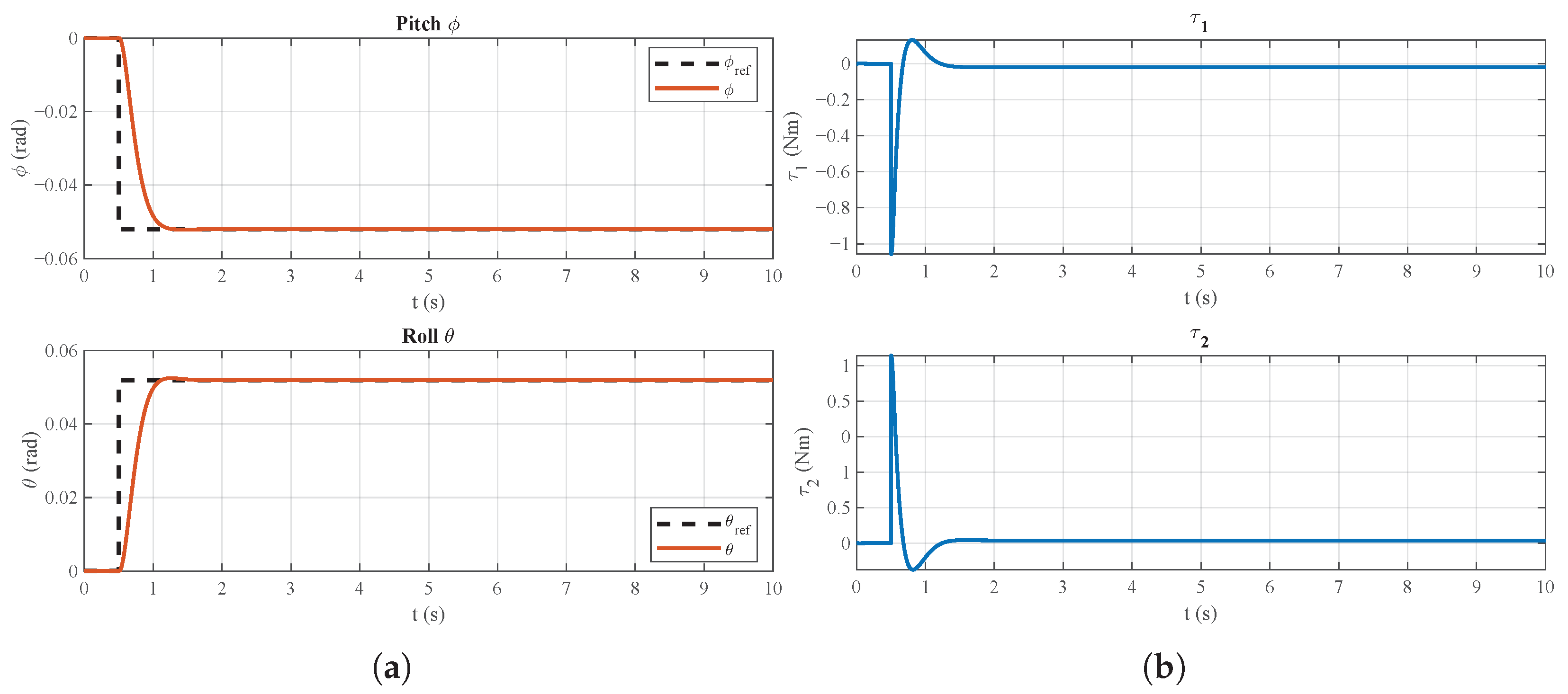
Following the optimization procedure, the tuned gain vector ${\mathbf{p}}^{★}$ was applied to the nonlinear closed-loop system. The time-domain responses are presented in Figure 4. This demonstrates rapid convergence of both pitch and roll angles with negligible steady-state error. The control torques remain smooth and bounded, without sustained saturation. These results validate the proposed closed-loop optimization framework for systematic PID tuning.

2.5. Linear Quadratic Regulator (LQR) Control

The LQR is a model-based optimal control strategy that minimizes a quadratic cost function that balances system-state deviations and control effort. For the balance board system dynamics represented in the linearized state-space form:

$$\dot{x}\left(t\right)=Ax\left(t\right)+Bu\left(t\right),y\left(t\right)=Cx\left(t\right)$$

(49)

The LQR controller determines the optimal feedback gain matrix K by minimizing the quadratic cost function:

$$J={\int }_0^{\infty }\left[x^T\left(t\right)Qx\left(t\right)+u^{\top }\left(t\right)Ru\left(t\right)\right]dt$$

(50)

Here, Q is a positive semi-definite weighting matrix for the states, and R is a positive definite weighting matrix for control input efforts. Once the optimal gain matrix K is obtained by solving the Algebraic Riccati Equation (ARE):

$$A^{\top }P+PA-PB{R}^{-1}{B}^{\top }P+Q=0$$

(51)

The control law is expressed explicitly as a state-feedback control:

$$u\left(t\right)=-Kx\left(t\right),\mathrm{where}K=R^{-1}{B}^{\top }P$$

(52)

2.6. LQR Parameter Tuning

The performance of an LQR controller significantly depends on the selection of weighting matrices Q and R. In this study, the selection and tuning of Q and R matrices are guided by practical considerations and simulation outcomes. The following general approach is adopted. Increasing the weights in the matrix Q for states associated with angular deviations (pitch and roll angles) yields tighter position control and reduced angular deviations but may increase control effort. Adjusting the weights in the matrix R regulates the magnitude of the control inputs. Higher values of R may lead to reduced control inputs, slower response, and larger steady-state errors.

A structured, iterative approach is employed, starting with equal-weighting matrices and progressively adjusting entries to achieve optimal performance. Optimal performance is evaluated based on minimal steady-state error, reduced oscillations, rapid settling time, and efficient disturbance rejection.

2.7. NAC Parameter Tuning

In the proposed neuro-adaptive controller, the sliding surface is defined as $s=\dot{e}+\lambda e$, where $e=q-q_d$ denotes the tracking error and $\lambda >0$ is the sliding-surface slope parameter. The parameter $\lambda$ directly determines the relative weight between position error and velocity error and therefore regulates the convergence rate of the closed-loop system. Under ideal sliding conditions ($s=0$), the error dynamics reduce to $\dot{e}+\lambda e=0$, which yields the exponentially stable solution.

$$e\left(t\right)=e\left(0\right)e^{-\lambda t}.$$

(53)

Thus, increasing $\lambda$ accelerates the nominal convergence rate of the tracking error. However, in the presence of model uncertainties and actuator limitations, excessively large $\lambda$ values may lead to aggressive control actions and increased control effort. To systematically evaluate this trade-off, a $\lambda$-sensitivity analysis was conducted over the range

$$\lambda \in [{\lambda }_{min},{\lambda }_{max}].$$

(54)

For each value of $\lambda$, the closed-loop system was simulated under identical reference trajectories and disturbance conditions. The following performance metrics were computed:

$$\begin{array}{cc}\hfill \mathrm{RMSE}& =\sqrt{{\displaystyle \frac{1}{T}}{\int }_0^T{e}^2\left(t\right)dt},\hfill \end{array}$$

(55)

$$\begin{array}{cc}\hfill J_u& =\sqrt{{\displaystyle \frac{1}{T}}{\int }_0^T{\parallel \tau \left(t\right)\parallel }^{2}dt},\hfill \end{array}$$

(56)

Here, RMSE denotes the root-mean-square tracking error and $J_u$ represents the root-mean-square control effort. The sensitivity results reveal a non-monotonic performance trend. While moderate increases in $\lambda$ improve tracking accuracy by accelerating error convergence, excessive values increase control effort and neural adaptation activity, potentially leading to oscillatory behavior and increased actuator saturation.

To visualize the trade-off between tracking performance and control effort, a Pareto curve was plotted with RMSE against $J_u$ for each $\lambda$. The results indicate the existence of an optimal operating region in which tracking accuracy is significantly improved without a disproportionate increase in control effort.

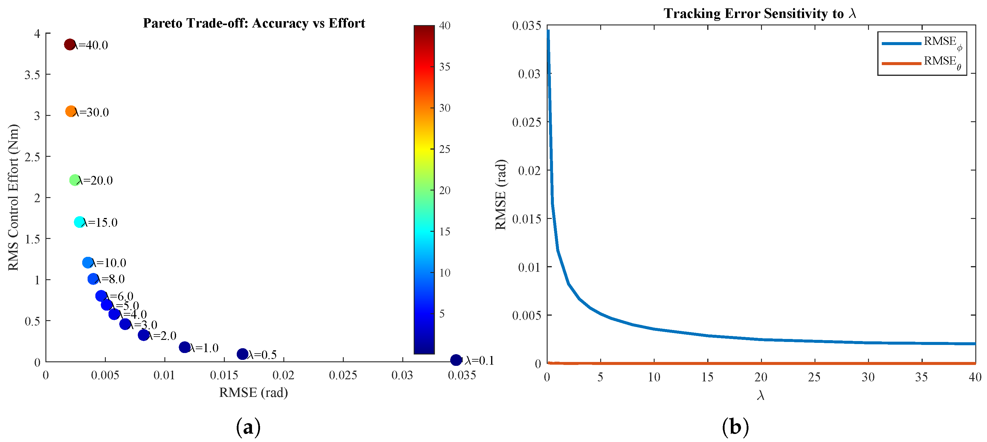
The results of the $\lambda$ sensitivity analysis are illustrated in Figure 5. As shown in Figure 5b, the RMSE decreases rapidly as $\lambda$ increases from small values, confirming the theoretical prediction that larger $\lambda$ accelerates exponential error convergence. The reduction in RMSE becomes progressively smaller beyond moderate values of $\lambda$, indicating diminishing returns in tracking performance. Meanwhile, the Pareto trade-off depicted in Figure 5a shows a monotonic increase in control effort $J_u$ as $\lambda$ increases. This trend reflects the increasing aggressiveness of the sliding surface $s=\dot{e}+\lambda e$, which amplifies corrective control actions. Importantly, the Pareto curve exhibits a clear knee region where a substantial reduction in RMSE is achieved with only a moderate increase in control effort. Beyond this region, further increases in $\lambda$ result in disproportionately large control effort with minimal improvement in tracking accuracy.

Based on this trade-off analysis, $\lambda$ was selected within the knee region of the Pareto curve, where tracking performance is near-optimal while maintaining practical actuator demands and bounded neural adaptation. This selection strikes a balance among convergence speed, robustness, and energy efficiency. In addition to the sliding surface parameter $\lambda$, the remaining NAC parameters were selected following stability, robustness, and bounded adaptation principles. The sliding-mode gains were chosen to dominate the bounded system uncertainty. Considering the sliding surface dynamics,

$$\dot{s}=-k_{1}s-k_2\mathrm{sat}\left(s\right)+\Delta \left(t\right),$$

(57)

where $\Delta \left(t\right)$ represents lumped uncertainty, the gains were selected such that

$$k_1,k_2>{\parallel \Delta \left(t\right)\parallel }_{max}.$$

(58)

This ensures exponential convergence of the sliding surface while preserving robustness against modeling errors and disturbances. The boundary layer thickness ${ϵ}_B$ was introduced to mitigate chattering effects. A moderate value was selected to balance steady-state accuracy and control smoothness. The neural adaptation gains (${\gamma }_{W1}$, ${\gamma }_{W2}$) were tuned to ensure sufficiently fast mismatch compensation while maintaining bounded weight evolution. Excessively large learning rates may lead to weight oscillations, whereas very small values slow adaptation. The selected values ensure stable convergence of weights under projection constraints. Weight projection limits were introduced to prevent parameter drift and ensure practical implementability. These bounds ensure that the neural weights remain within a compact set, thereby preserving closed-loop stability. Selected parameters are shown in the Table 1.

3. Results and Discussion

The performance of the NAC was evaluated with comparative simulations against traditional PID and LQR controllers. Simulations were conducted using a nonlinear balance-board model implemented in MATLAB R2025b. Tracking performance, control effort, and the interaction between axes were analyzed.

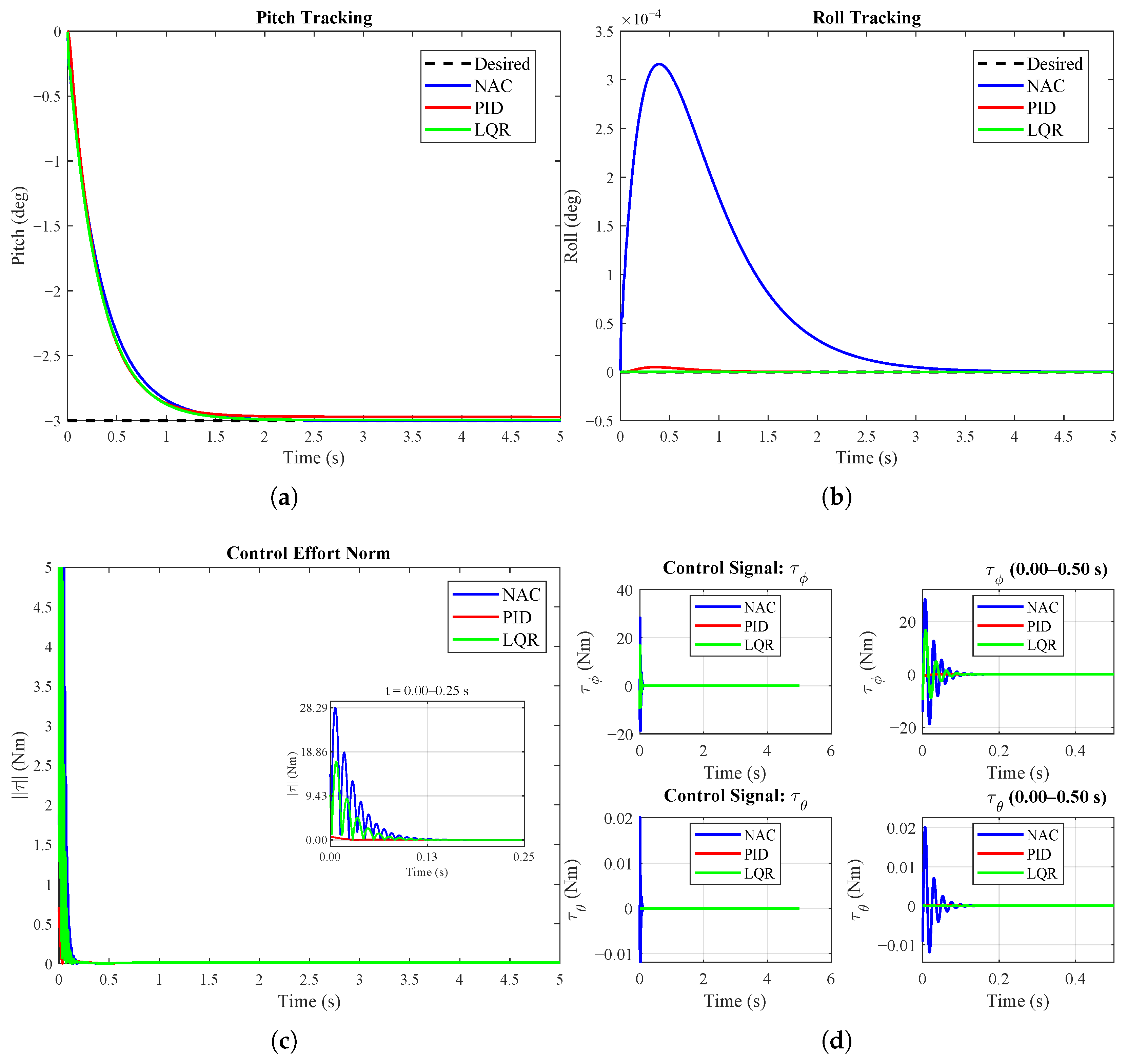
The simulations were initiated without any parameter uncertainty or external disturbances. In this case, the balance board was commanded to track a $-3^{\circ }$ step reference in pitch and maintain a roll angle of $0^{\circ }$.

Figure 6a shows the pitch angle responses of the NAC, PID, and LQR controllers. All controllers successfully track the reference under nominal conditions. Steady-state errors are negligible, and settling times are comparable. There is no important performance difference between the controllers. These results are as expected, as the plant dynamics are fully known and there is no uncertainty.

Figure 6b shows the response of the roll angle while the pitch angle is commanded to the step reference. Although there are small deviations in the roll angle, especially at the beginning of the simulation, the magnitude of these deviations is about ${10}^{-4}$ degrees. These values are negligible in practice and indicate that the controllers interact only during the initial peak effort.

Although NAC shows a brief transient rebound in the control effort norm shown in Figure 6c, and control signals shown in Figure 6d, it achieves a faster attenuation.

Table 2. Quantitative comparison of control-effort metrics.

Controller	Settling Time (s)	Control Energy (${\int \parallel \mathit{u}\left(\mathit{t}\right)\parallel }^2\mathbf{dt}$)	Post-Settling RMS (Nm)
NAC	$0.264$	$2.0085$	$0.018022$
PID	$0.475$	$0.026571$	$0.017993$
LQR	$0.301$	$0.56557$	$0.018006$

shows that NAC yields a shorter settling time. The short rebound in NAC is caused by the online adaptation law’s compensation for modeling mismatch and disturbance, leading to a brief corrective action when the tracking error crosses a small neighborhood around zero.

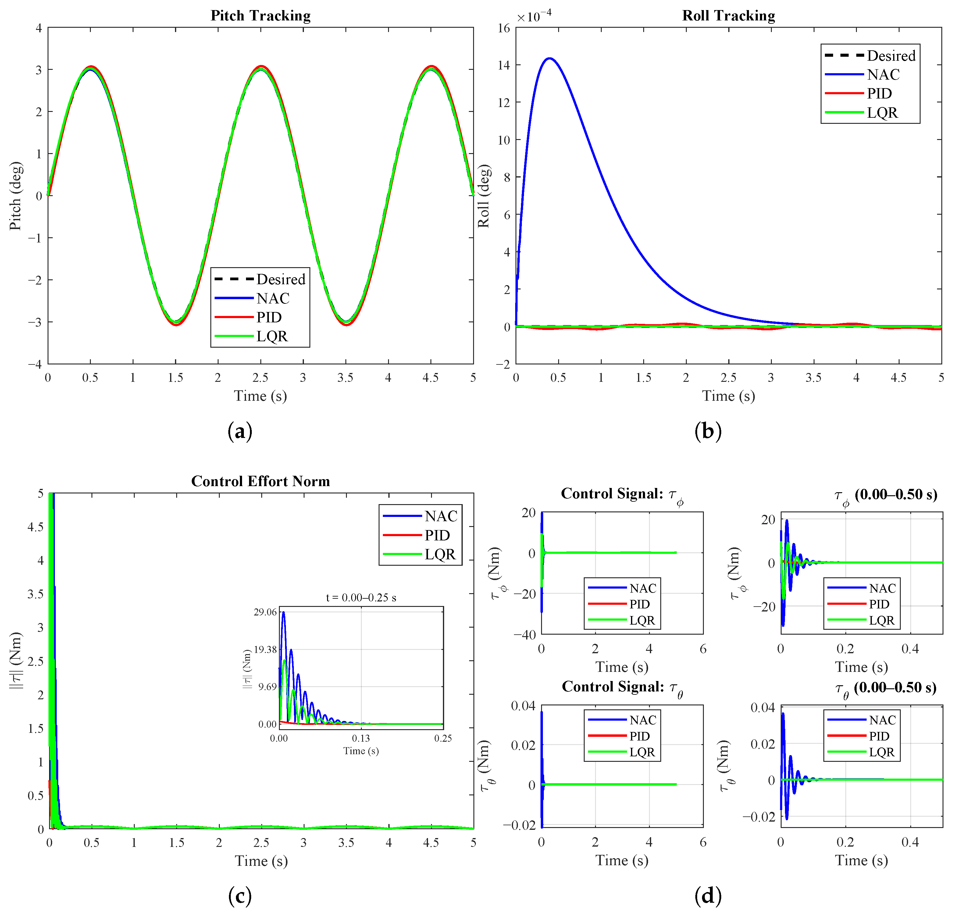
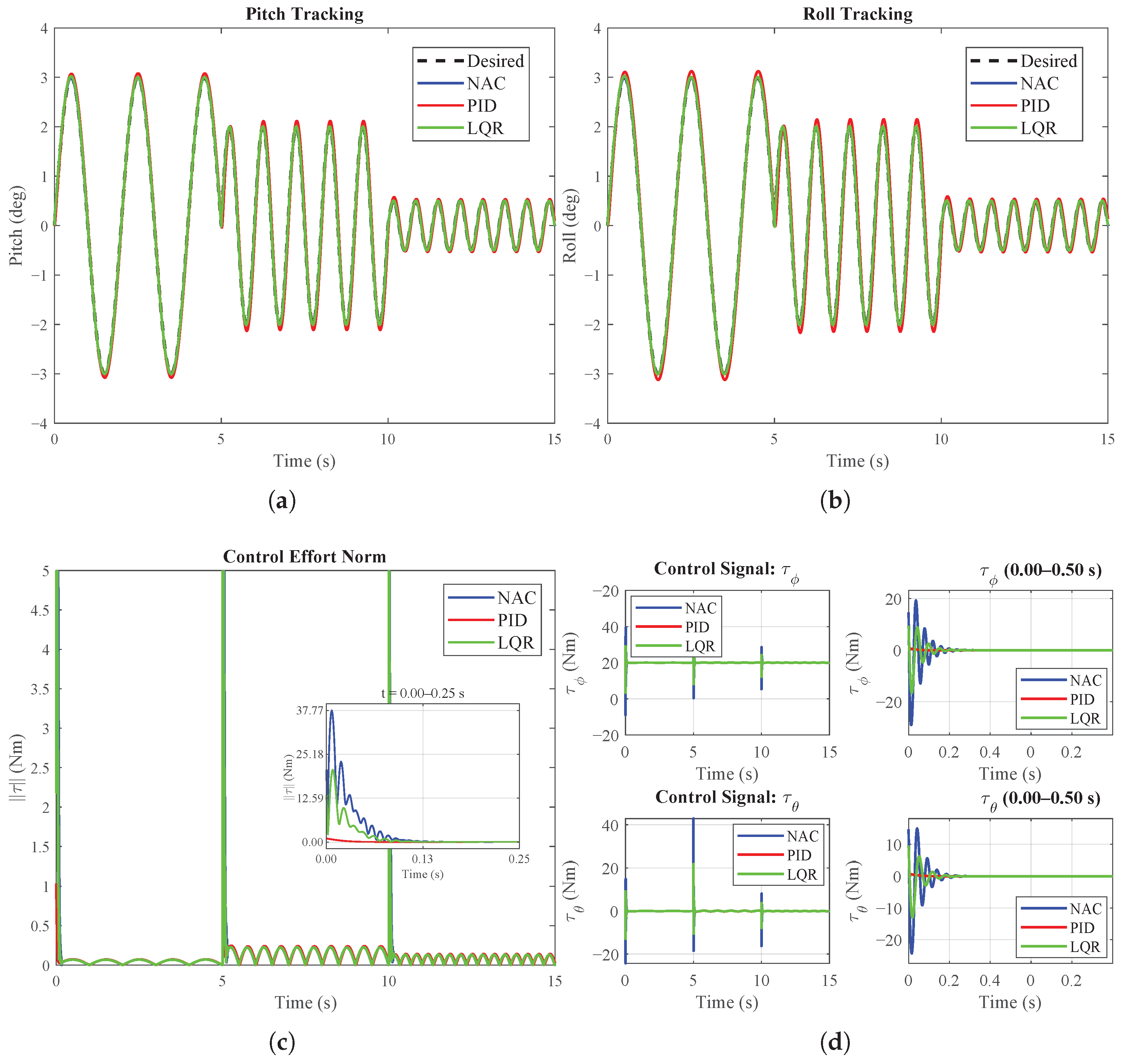
The dynamic tracking performance of controllers was evaluated using fixed-frequency sinusoidal reference signals. The maximum amplitude of the reference signals was $\pm 3^{\circ }$ degrees for these tests. This test aimed to assess controller behavior under continuously varying references and to examine cross-axis coupling effects.

Figure 7a presents the angular responses of NAC, PID, and LQR controllers to the sinusoidal reference. It can be seen that all controllers successfully track the reference, but the PID controller exhibits an obvious amplitude error and a phase lag, particularly near the peaks. Even though LQR tracks the reference more accurately than PID, it exhibits small-magnitude deviations. The proposed NAC controller exhibits the best phase performance and minimizes magnitude deviations.

Figure 7b shows the roll angles that were required to remain regulated at 0. The cross-interaction caused by the sinusoidal reference is observed in this axis. The PID controller induces pitch-axis oscillations and cannot suppress cross-axis interactions during sinusoidal excitation. On the other hand, the NAC controller can more effectively suppress inter-axis interactions.

Figure 7c shows the control efforts, and Figure 7d shows control signals for all controllers. All three controllers generate periodic control inputs in response to the sinusoidal reference. There is no clear observation of the differentiation in the magnitude of control effort between controllers. However, NAC’s tracking performance did not require additional control effort.

Figure 8 illustrates the responses of the balance board to a variable frequency sinusoidal reference under nominal conditions. This test evaluates the controller’s adaptability to a time-varying reference.

Figure 8a,b show the tracking performance of controllers for pitch and roll axes, respectively. All controllers successfully track the reference signal. Despite the reference frequency increasing over time, no unstable behavior is observed for any of the control strategies. Figure 8c,d show the control efforts and control signals for the controllers.

There is no clear difference in tracking performance between controllers. These behaviors reflect the fact that the system dynamics are well known under nominal conditions.

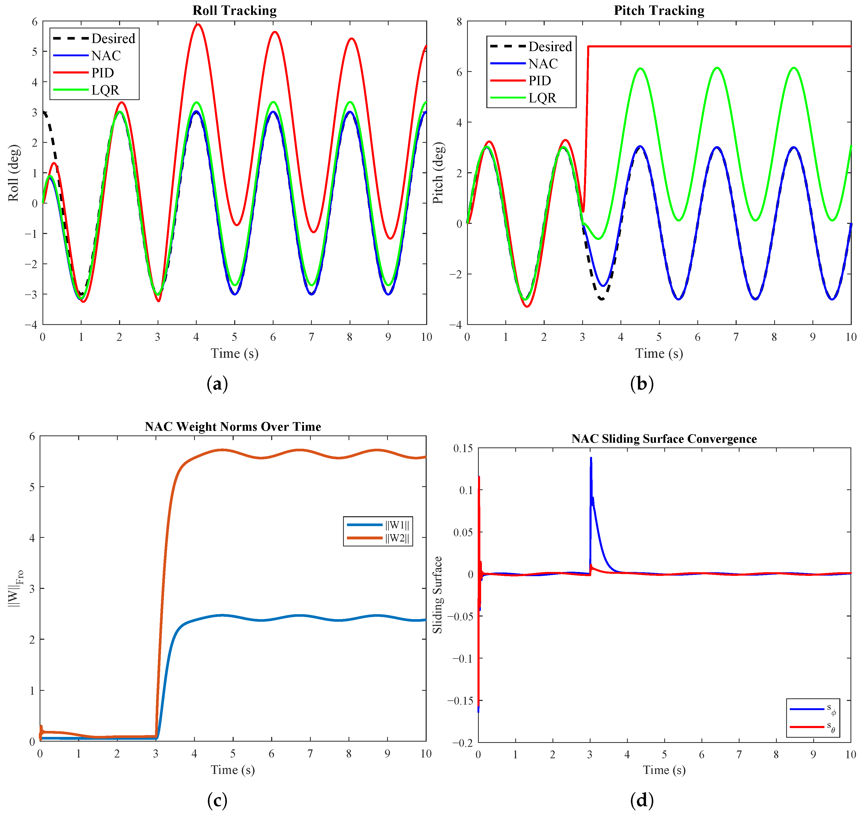
Figure 9 presents the controller responses under parameter uncertainty and external disturbances. Two disturbance scenarios were considered. A 1 Nm step disturbance was applied to the roll axis starting at the 3rd second of the simulation. In addition, the pitch axis was commanded by a fixed-frequency sinusoidal reference, and a stronger 10 Nm disturbance was introduced again at the 3rd second to evaluate robustness under severe conditions.

Figure 9a shows the controller performances under 1 Nm disturbance and uncertainty. The PID controller produces large deviations under disturbance. The LQR controller partially suppresses these deviations, but a steady-state error persists. The NAC controller effectively regulates the roll angle, even in the presence of parameter uncertainty and external disturbances.

The pitch responses are shown in Figure 9b. All controllers can track the reference with acceptable performance before the disturbance is applied. However, when the 10 Nm disturbance is applied, the limitations of classical controllers become more evident. The PID controller exhibits significant deviation from the reference and reaches the mechanical saturation limits, degrading tracking performance. Although the LQR controller outperforms the PID controller, noticeable tracking errors and oscillations persist under high-disturbance conditions. In contrast, the NAC controller maintains a bounded tracking error and recovers faster after the disturbance.

The adaptive behavior of the NAC controller is illustrated in Figure 9c through the neural network weight norms. Immediately after the disturbance is applied, the weights adjust to compensate for the altered system dynamics. After this transient phase, the weights remain bounded within a limited range, indicating stable online adaptation.

Figure 9d shows the evolution of the sliding surfaces for both axes. Following the disturbance, the sliding variables rapidly converge toward zero, confirming the stability and robustness of the NAC controller under uncertainty and large external disturbances.

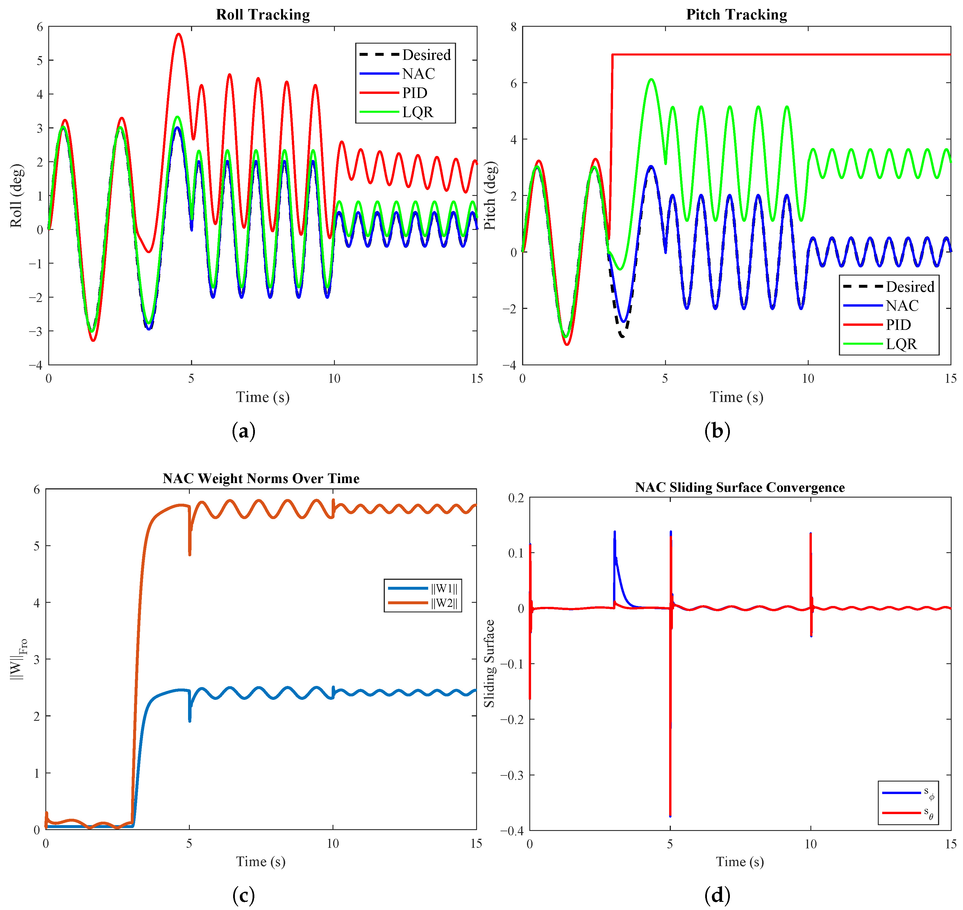
Figure 10 shows the controller responses under parameter uncertainty and external disturbances in a variable-frequency reference-tracking scenario. Two disturbance levels were considered. A 1 Nm step disturbance was applied to the roll axis starting at the 3rd second of the simulation. In addition, a stronger 10 Nm disturbance was introduced to the pitch axis at the same instant to evaluate robustness under more severe conditions.

Figure 10a illustrates the roll-tracking performance. Under the lower 1 Nm disturbance, noticeable amplitude deviations and phase shifts are observed in the classical controllers due to parameter uncertainty interacting with frequency variations. The PID controller shows increasing oscillation amplitude and phase mismatch. The LQR controller performs better than PID, yet small but persistent tracking errors remain. In contrast, the NAC controller maintains a bounded tracking error and more consistent amplitude behavior across varying reference frequencies.

The pitch responses are shown in Figure 10b. When the 10 Nm disturbance is applied, the limitations of the classical controllers become more pronounced. The PID controller exhibits large deviations and reaches the mechanical limitations under the combined effects of parameter uncertainty and high disturbance. Although the LQR controller partially mitigates this deviation, steady amplitude errors persist. The NAC controller regulates the pitch motion more effectively and recovers faster after disturbance injection while keeping the response bounded.

The adaptive behavior of the NAC controller is illustrated in Figure 10c through the neural network weight norms. Immediately after the disturbances are applied, the weights adjust to compensate for the altered and uncertain dynamics. Following this transient adaptation phase, the weights remain bounded within a finite interval, indicating stable and continuous online adaptation.

Figure 10d shows the evolution of the sliding surfaces for both axes. After the disturbance onset, the sliding variables rapidly converge toward zero and remain bounded around the sliding manifold. This behavior confirms the stability and robustness of the NAC controller under parameter uncertainty and asymmetric disturbance levels.

In this study, all tests were conducted under the same conditions, and all controllers yielded the same results. It is suggested that if the system dynamics are well known, traditional control algorithms remain effective. However, under parameter uncertainty and external disturbances, the performance of the PID and LQR controllers degraded significantly. The NAC controller maintained its tracking performance and closed-loop stability due to its online adaptation mechanisms. The limited, stable evaluation of the neural network and the convergence of the sliding surface variables confirm that NAC effectively adapts to uncertainties and disturbances.

4. Conclusions

In this study, a neuro-adaptive sliding mode controller was developed for a balance board system driven by pneumatic artificial muscles (PAMs). The proposed control method was compared with classical PID and optimal LQR controllers in both step-tracking and sinusoidal-tracking scenarios.

The results showed that while the PID controller ensured basic tracking, it required high control effort and responded slowly to changes. The LQR controller improved performance slightly but lacked adaptability under varying dynamics. In contrast, the Neuro-Adaptive Controller (NAC) achieved faster convergence to the reference and better handled overall system uncertainties.

Lyapunov-based analysis confirmed the theoretical stability of the NAC, and the use of a neural network allowed the controller to adjust to unknown dynamics in real time. Synthetic step response scenarios, scaled from experimental data, further validated the control strategy and showed its potential for real-world application.

In conclusion, the neuro-adaptive approach is a promising solution for soft-actuated rehabilitation systems, offering adaptability, efficiency, and stability. Future work will focus on full experimental validation and clinical integration of the proposed system.