Experimental Research on the Supercooling and Freezing Temperatures of Unsaturated Soil

Highlights

• The freezing and supercooling temperatures of soil are critical parameters for accurately determining its phase state and physico-mechanical properties.
• An elevated ambient cooling rate induces pronounced boundary effects, which subsequently suppress the supercooling phenomenon at the center of the soil sample.
• Compared to traditional thermocouple techniques, the proposed method offers a more practical solution, achieving a superior balance between measurement efficiency (time) and accuracy.

Abstract

With the development of polar regions and the deepening utilization of cold region resources, a large number of infrastructure projects are continuously being carried out. The freezing temperature of unsaturated soil is a critical factor governing the freezing depth and stability of foundations in cold regions or seasons. Concurrently, the supercooling state of soil significantly influences the assessment of its phase composition and physico-mechanical properties. This study employed physical experiments, theoretical formulas, and numerical simulations to reveal the influencing factors and underlying mechanisms of supercooling characteristics in unsaturated soils under controlled low-rate continuous cooling conditions. The results demonstrate that a reduced temperature gradient between the sample surface and the ambient environment correlates with a lower supercooling limit temperature and an extended supercooling duration. An excessively high cooling rate suppresses the supercooling phenomenon in the sample core due to boundary effects. In contrast, neither the temperature difference nor the external cooling rate exhibit a negligible influence on the freezing temperature. Analysis of the temperature–time curves reveals that the freezing process of silty clay is more stable, exhibiting fewer stepwise temperature declines during the phase change plateau, whereas mudstone shows heightened sensitivity to variations in the thermal gradient. Compared to conventional thermocouple measurements, the proposed methodology achieves an optimal balance between temporal efficiency and measurement accuracy. It not only enhances experimental controllability and data reliability, but also provides more scientific theoretical support and technical pathways for predicting freezing depth, designing foundation thermal systems, and preventing frozen ground disasters in cold region engineering.

1. Introduction

Seasonal climate change leads to freeze–thaw cycles in permafrost and seasonally frozen soil, altering their physical states and significantly affecting soil mechanical parameters [1,2]. Engineering construction in frozen regions disturbs permafrost, disrupts its thermal equilibrium, and leads to permafrost degradation, consequently inducing road frost heave and thaw settlement [3,4,5,6,7]. Freezing temperature is the key physical parameter for determining soil freezing conditions, serving as the basis for calculating both subgrade freezing depth and artificial freezing wall thickness [1,8], and is a key factor influencing moisture migration and frost deformation in frozen soil [9,10]. Based on the work of former Soviet scholar Tsytovich regarding the subzero temperature state of frozen soil, the water-ice phase transition process can be categorized into three zones: the intense phase transition zone, the transition zone, and the frozen solid zone [11]. During soil freezing, a temperature decrease of 1 °C resulting in more than 0.1% of the pore water converting to ice indicates that the soil sample has entered the frozen state. Upon reaching a specific subzero temperature, the soil attains a chilled state. This is characterized by a stabilized multiphase composition, where the unfrozen water content remains nearly constant despite further decreases in temperature [12,13,14,15,16]. Additionally, under certain conditions, soil can undergo supercooling during the freezing process. When the soil temperature falls below the freezing point, the pore water may not freeze immediately. Phase transformation is delayed until the ambient temperature drops further, at which point the soil temperature exhibits a sudden rise. This phenomenon occurs due to the nucleation and crystallization of both free and bound water in the soil. Specifically, some water molecules aggregate and arrange into ice-crystal nuclei, while others accrete to form ice-crystal clusters [17,18,19]. Upon further cooling to a critical temperature, the pore water undergoes phase change, releasing latent heat (approximately 332.9 J·g⁻¹). This release induces a sudden temperature rise, which subsequently maintains a stable plateau. The occurrence of this distinct thermal response, characterized by rapid warming followed by thermal stabilization, confirms the manifestation of soil supercooling.

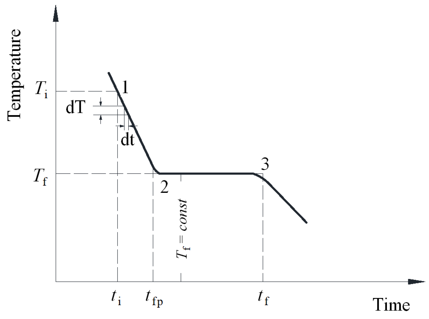
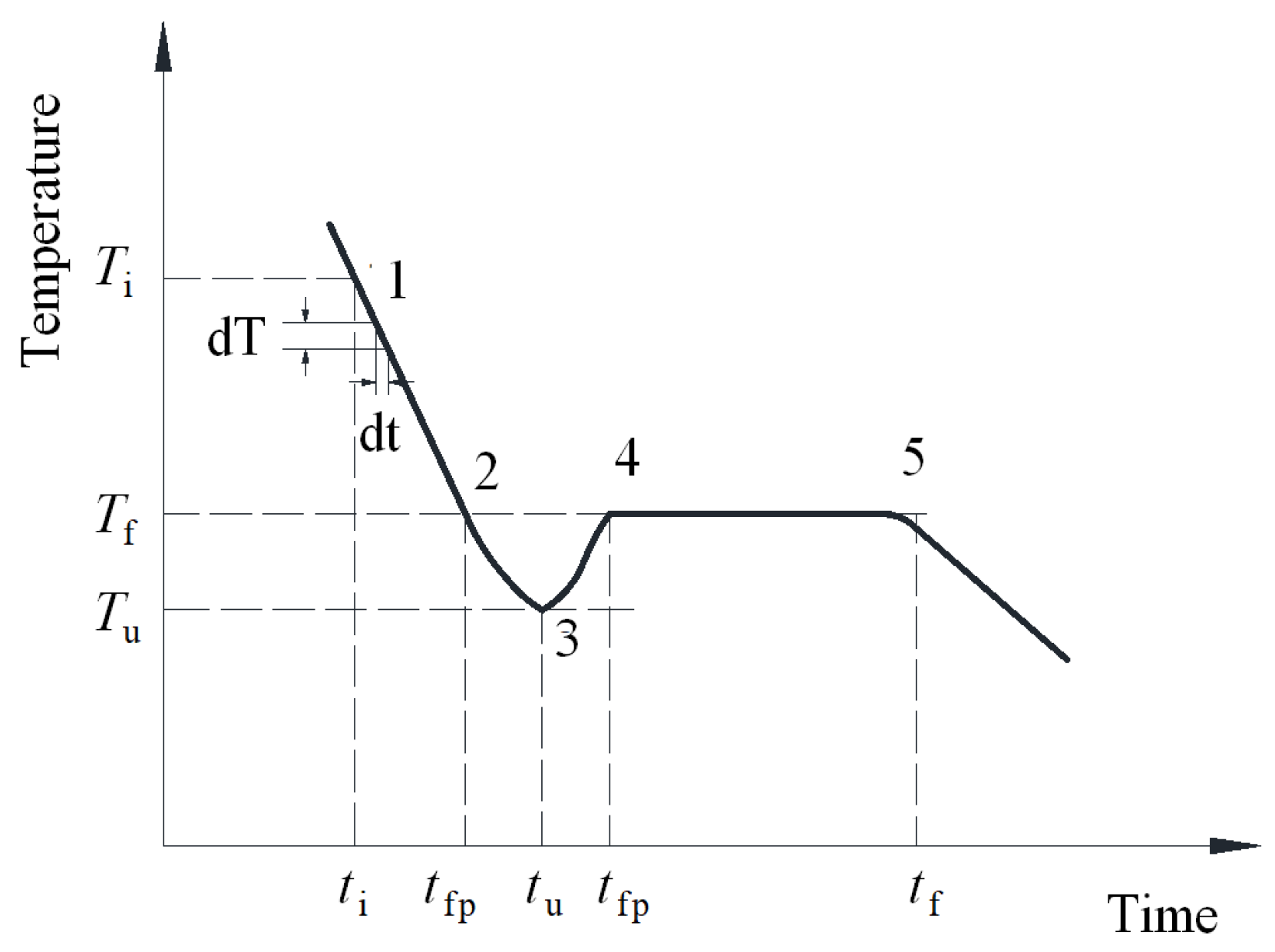
Factors influencing soil freezing temperature and unfrozen water content have been extensively investigated by numerous scholars. Liu et al. introduced an electrical potential transition method to determine the freezing temperature of wet soil, subsequently using it to investigate the relationships between freezing temperature and pressure, moisture content, and wet bulk density [20]. Yao et al. examined the influence of the freezing phase transition temperature on frozen wall thickness formation under varying strata, water contents, and external loading conditions [21,22,23]. Wan et al. developed and validated a calculation model for determining unfrozen and residual water content in freezing soil [17]. Leng et al. analyzed factors affecting unfrozen water content, including negative temperature, soil type, and initial water content [24]. Zhou et al. developed a novel experimental apparatus for determining soil freezing temperatures using ultrasonic nucleation induction technology and solid-state refrigeration technology. The study investigated the effects of size effects and supercooled states on freezing temperatures [25]. Li established a calculation model and testing method for determining the unfrozen water content of small-volume frozen soil samples [26]. Ying proposed a thermodynamically consistent equilibrium temperature formula that incorporates the effects of water activity and pore radius [27]. Experiments by Zhou and Xu on non-salinized soils indicated that the freezing characteristic curve is independent of initial water content, and that different cooling modes and rates exert no significant effect on the freezing temperature [28,29]. Chen et al. measured brine temperatures and surface subsidence, numerically modeled the freezing wall temperature field distribution using finite element analysis, and demonstrated the effectiveness of adding an inner circle of freezing holes for achieving lower temperatures, thereby facilitating subsequent shaft excavation [30]. Shan et al. analyzed the thermal characteristics of loamy silt with different initial moisture contents during freezing and thawing cycles using Differential Scanning Calorimetry (DSC) experiments [4]. Liu conducted NMR measurements on remolded loess during controlled cooling to obtain T₂ spectra at target temperatures, based on soil freezing characteristics [31]. Soil freezing point decreases with decreasing water content [32,33,34,35]. Additionally, while changes in the thaw front and soil moisture thaw period were synchronous, the moisture freezing period exhibited significant hysteresis relative to ground temperature changes [36]. Based on artificial ground freezing experiments, Tounsi reported that pore water expansion during freezing and the resulting pressure can induce ground movements in adjacent non-frozen areas [37]. Although the concept of supercooling has been mentioned in the literature, the supercooled state of soils remains poorly studied. Figure 1 and Figure 2 present temperature-time curves for soil freezing without and with supercooling, respectively. A distinct temperature jump is evident in the supercooling section of the curve. The onset of this temperature jump is defined as the limiting supercooling temperature, while its endpoint is identified as the freezing point. The presence of supercooling means that the freezing state of soil cannot be determined based on the freezing temperature alone. Ignoring the soil’s undercooled state can lead to misjudgment of its phase state and physico-mechanical properties. Therefore, a comparative study of soil supercooling temperature and freezing temperature is crucial, yet such research remains scarce.

In the design of infrastructure projects in cold regions, relying solely on empirical knowledge has significant limitations. Supercooling occurs only during the freezing stage and is absent during the thawing stage. Therefore, to determine hysteresis in the freeze–thaw cycle, an experimental assessment of supercooling is necessary. This study employs the lumped parameter method and continuous cooling method to systematically elucidate the combined effects of volumetric parameters and temperature gradients on freezing and supercooling temperatures [38,39]. Accordingly, a novel low-rate heat transfer method based on natural air convection is proposed. By measuring temperatures at key representative points within three types of small-volume soil samples of different specifications, the average soil temperature is approximated, enabling systematic observation of the entire supercooling and freezing processes. The temperature was controlled from −25 °C to 20 °C, covering the typical range of ground temperature variations in cold regions. Relevant test results are crucial for elucidating the mechanical and thermal response mechanisms of frozen ground during freezing and thawing cycles. This research is expected to provide theoretical support for “temperature-controlled design of frozen ground foundations,” “precise quantification of soil physical properties during the initial stage of artificial ground freezing,” and “the frost resistance characteristics of unsaturated soils in numerical calculation models for engineering projects in cold regions.”

2. Experimental Equipment and Methods

2.1. Experimental Equipment

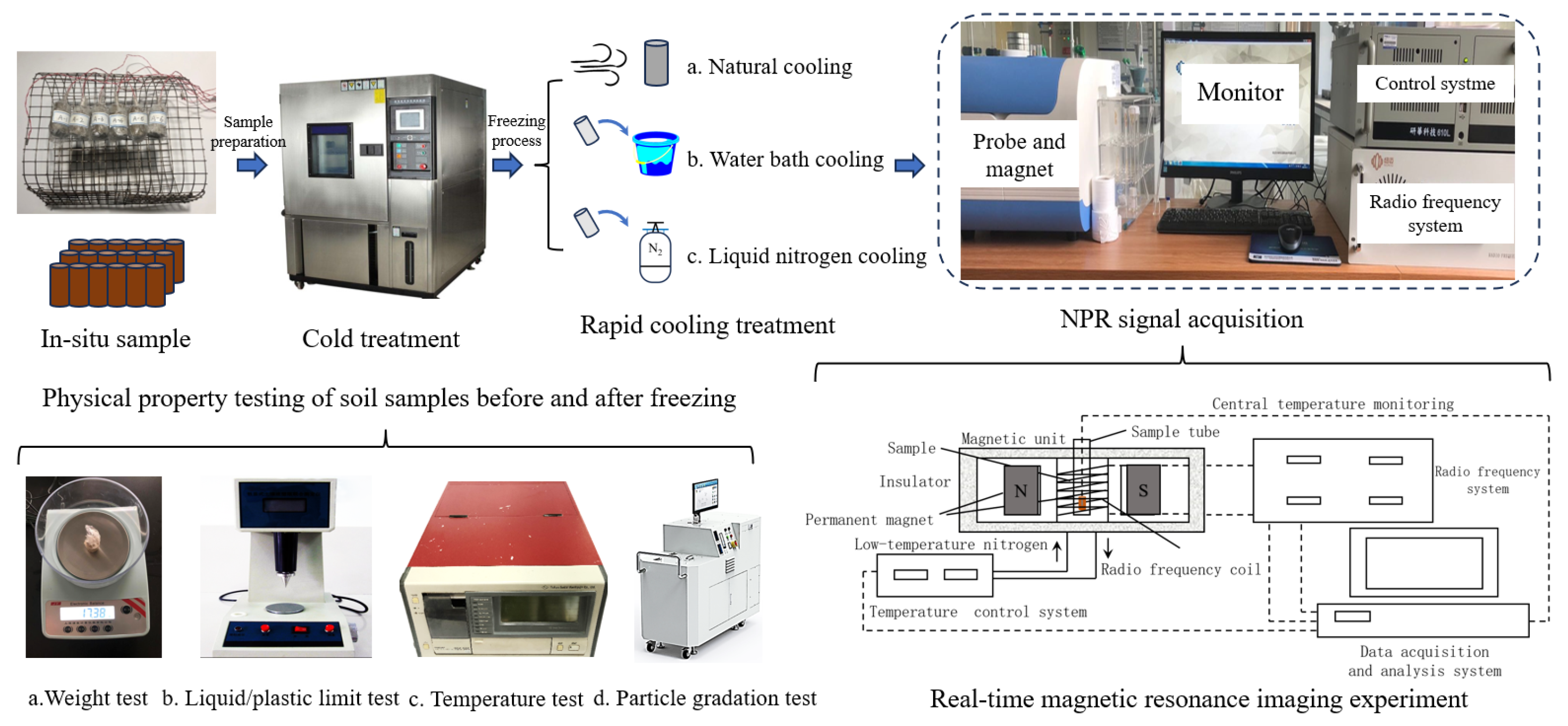
Standardized equipment and methods for measuring soil freezing temperature have been established [40,41,42]. A low-temperature, constant-temperature environment was traditionally created by mixing natural ice with a saline solution in a specific ratio. The soil sample temperature was measured using thermocouples at various time intervals, and the freezing temperature was determined from the inflection point of the resulting temperature-time curve. However, this conventional setup offers limited flexibility for precise ambient temperature control, making it difficult to investigate soil supercooling and freezing temperatures under continuous cooling conditions. In this study, a programmable constant temperature and humidity chamber was employed to provide a precisely controlled low-temperature environment. The temperatures of both the soil sample and the chamber air were measured in real time using temperature sensors connected to a data acquisition system. Cylindrical soil samples were prepared. A temperature sensor was inserted into the center of each sample, which was then sealed with plastic film and placed inside the climate chamber. The temperature sensors had an accuracy of ±0.05 °C. A separate sensor monitored the chamber air (ambient) temperature. All sensors were connected to a data acquisition unit, which transmitted the data to a computer. Acquisition software on the computer recorded both soil and ambient temperatures in real time. The unfrozen water content in soil at various temperatures was measured using nuclear magnetic resonance (NMR). The unfrozen water content-temperature curve obtained from NMR was then compared with the temperature-time curve from the freezing experiment to elucidate the influence of supercooling temperature on soil phase state. A schematic of the experimental setup is presented in Figure 3.

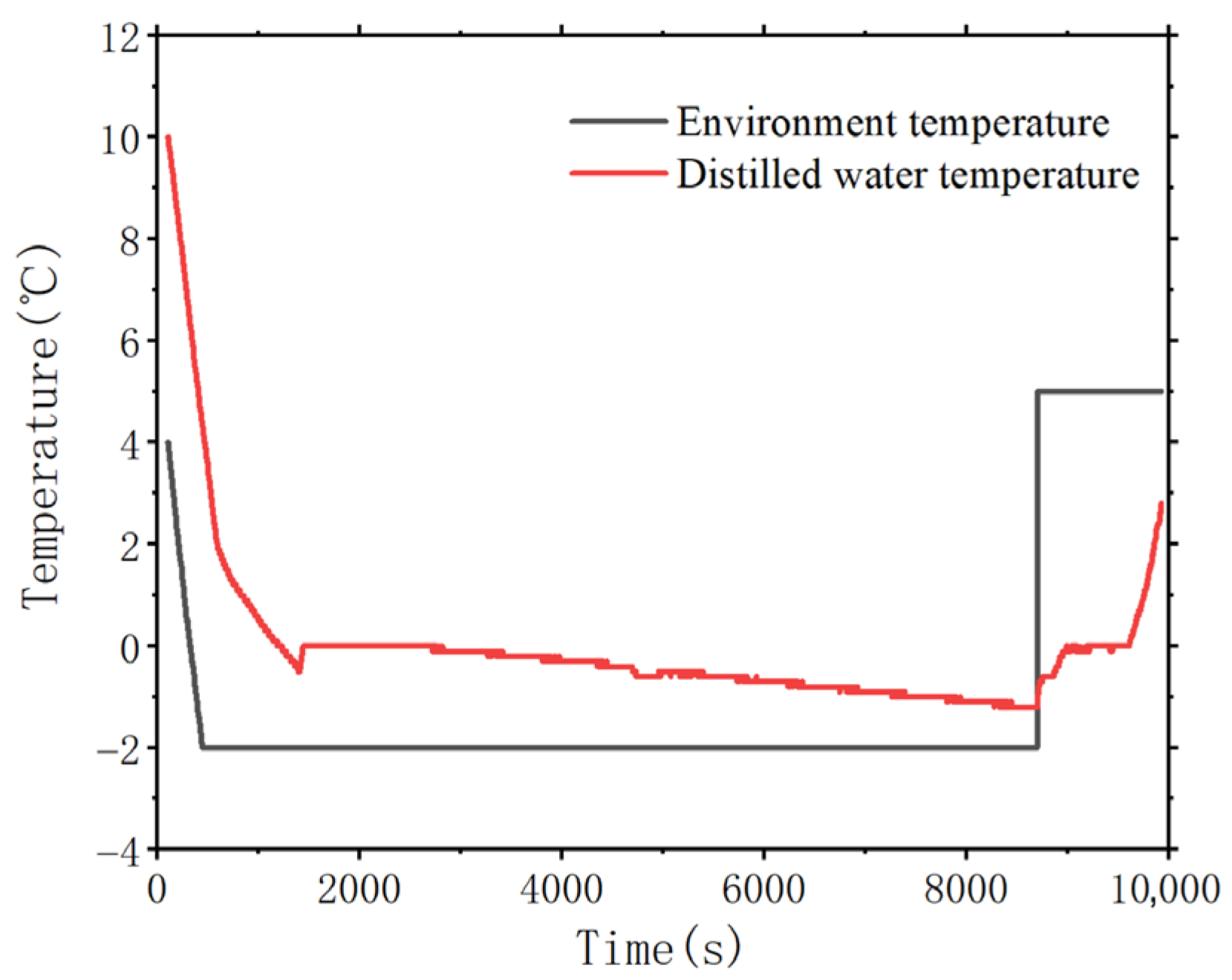
To verify sensor precision and test result accuracy, a freeze–thaw cycle was performed on distilled water within the programmable climate chamber. The resulting temperature-time curve is shown in Figure 4. The freezing curve of distilled water reveals a distinct supercooling phase. Following a sudden temperature increase, the curve stabilizes at a plateau of 0 °C, which is the equilibrium freezing point of pure water. This agreement with the theoretical value confirms the high reliability of the experimental apparatus. In contrast, the melting process shows no analogous sudden temperature change or “overheating” phenomenon, highlighting a fundamental thermodynamic asymmetry with the freezing process.

2.2. Specimen Preparation

Silty clay, red clay, and mudstone were selected for this study. The soil samples were oven-dried as an initial preparation step. To achieve target water contents of 22%, 28%, and 38%, deionized water was added to the dried soils. The mass of water required for each target moisture content was calculated based on the dry soil mass. After thorough mixing, each soil-water mixture was sealed in a plastic bag and cured at approximately 25 °C for 24 h to ensure uniform moisture distribution. Each soil mixture was compacted into a mold in three layers. For each soil type, seven specimens of varying dimensions were prepared (see

Table 1. Specimen dimensions.

Parameter	A	B	C	D	E	F	G
d/mm	32	32	32	32	20	20	20
h/mm	47	31.33	23.5	15.67	30	20	15
V/mm3	37,780	25,184	18,584	12,596	9420	6280	4710
A/mm2	6330	4755	3968	3181	2512	1884	1570
l/mm	5.9682	5.2956	4.7595	3.9570	3.75	3.33	3
B (<0.1)	0.0445	0.0395	0.0355	0.0295	0.0279	0.0248	0.0224
Quantity	4	4	4	4	4	4	4

). First, select specimens from Groups A and E with dimensions of 32 mm diameter × 47 mm height and 20 mm diameter × 30 mm height (aspect ratio 1.5), respectively. For other components, choose specimens with heights corresponding to 2/3, 1/2, and 1/3 of the 47 mm and 30 mm heights as distinct groups. Calculate parameters such as surface area and volume for each group.

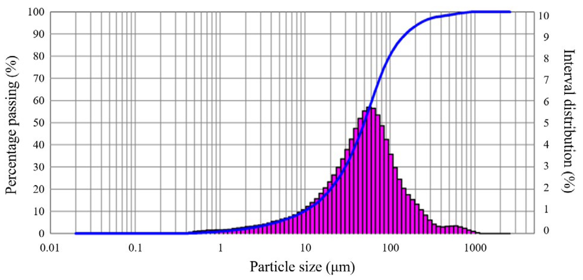
The particle size distribution of the silty clay is presented in Figure 5. Its liquid limit (W_L), plastic limit (W_P), and plasticity index (I_P) are 9.76%, 25.01%, and 15.25, respectively. The corresponding geotechnical parameters for the other soils are summarized in

Table 2. Geotechnical control parameters of test soils.

Soil	Plastic Limit (%)	Liquid Limit (%)	Plastic Index (Ip)	Grain-Size Distribution (%)
				<0.002	0.002~0.005	0.005~0.075	>0.075
Silty clay	9.87	24.01	14.14	3.45	9.04	69.29	18.22
Red clay	9.63	29.45	19.82	4.67	12.03	74.11	9.19
Mudstone	25.88	55.71	29.83	19.73	21.64	54.05	4.58

. The dry densities of the silty clay, red clay, and mudstone were maintained at 1.44 g/cm³, 1.38 g/cm³, and 1.25 g/cm³, respectively. In all experiments, the temperature sensors were positioned at the geometric center of each soil specimen, with the test duration lasting 40–45 min.

3. Experimental Results and Analysis

The existing freezing point ideas reveals that soil freezing is a gradual process occurring within a specific subzero temperature range, accompanied by the presence and migration of unfrozen water [1]. It serves as the theoretical foundation for understanding all geotechnical phenomena related to frozen ground, including frost heave, thaw settlement, and permafrost strength. The freezing point of soil water is typically below 0 °C due to complex interactions between soil particle adsorption, electrolytes, external pressure, gravity, and electrostatic forces. These factors allow the soil solution to remain liquid at temperatures below 0 °C, i.e., in a state of supercooling. This metastable state during phase transitions occurs because a lower temperature is required for the soil solution to transition to a stable state due to the thermodynamic potential barrier to nucleation. Reducing the ultimate supercooling temperature of soil and increasing the duration of supercooling can mitigate the effects of short-term freeze–thaw cycles caused by abrupt changes in meteorological conditions.

3.1. Analysis of Temperature Field Uniformity

Frozen soil is a four-phase system comprising soil particles, unfrozen water, ice, and air. Under subzero conditions, a portion of the pore water remains unfrozen. During the supercooling stage, the pore water persists in a liquid state despite temperatures falling below the equilibrium freezing point. Consequently, the unfrozen water content remains equivalent to the initial total water content. Therefore, accurately determining the soil’s freezing state throughout the freeze–thaw cycle is fundamental to this study. Achieving a uniform temperature field during the process is critical for this determination.

This study utilizes the lumped parameter method derived from heat transfer theory. The internal temperature evolution of small-volume soil specimens during freeze–thaw cycles was monitored to analyze the extent and mechanisms of soil freezing. This study employs the lumped parameter method from heat transfer theory. By monitoring the internal temperature evolution of small-volume soil specimens during freeze–thaw cycles, we analyze the extent and implications of soil freezing. The lumped parameter method applies when the internal temperature gradient within an object is negligible. This condition is met when the external convective thermal resistance significantly exceeds the internal conductive thermal resistance. Under such conditions during transient heat conduction, the entire sample can be considered isothermal at any given time. Consequently, the internal temperature distribution becomes a function of time alone, independent of spatial coordinates. Thus, the temperature field within the object is spatially uniform. This method enables rapid and accurate observation and analysis of the effects of temperature gradients on freezing and supercooling temperatures. The lumped parameter method treats the object as having a spatially uniform temperature. It assumes that physical properties, such as heat capacity, are lumped at a single point, allowing the temperature at any location to represent the overall temperature of the object [43]. Prior to experimentation, the applicability of the lumped parameter method must be validated. This is achieved by calculating the Biot number (Bi), a key dimensionless parameter defined as the ratio of internal conductive thermal resistance to external convective thermal resistance.

$$Bi={\displaystyle \frac{h{l}_e}{{\lambda }_s}}$$

(1)

where h is the convective heat transfer coefficient at the object surface (W·m⁻²·K⁻¹); l_e is the characteristic length (m): for an infinite plane wall, l_e = δ (the wall thickness); for an infinite cylinder or sphere, l_e = d/2 = R; and λ_s is the thermal conductivity of the solid (W·m⁻¹·K⁻¹).

When Bi approaches zero, it signifies that the external thermal resistance (r₀) is significantly greater than the internal conductive resistance (r_i). Consequently, the internal thermal resistance of the solid can be neglected. Under this condition, the temperature within the object remains spatially uniform at any given moment. Over time, the overall sample temperature approaches that of the cold source. Thus, the sample’s temperature distribution depends solely on time as a single variable and is independent of spatial position. Conversely, when Bi→∞, it indicates that r₀ << r_i. In this case, the external convective thermal resistance is negligible. Consequently, the surface temperature of the object instantaneously reaches the cold source temperature at the initial moment. As time progresses, the temperature at every point within the body converges toward the cold source temperature. For finite values of Bi, neither the external heat transfer resistance nor the internal conduction resistance can be neglected. The resulting temperature field within the sample exhibits characteristics intermediate to the two limiting cases described above. Therefore, a prerequisite for applying the lumped parameter method is that the internal thermal resistance of the solid must be negligible. In engineering practice, the lumped parameter method is typically considered applicable when the relative temperature variation within the object is less than 5%, which corresponds to a Biot number of Bi ≤ 0.1. As an example, the Biot number is calculated for a silty clay sample with a height (H) of 47 mm and a radius (R) of 16 mm.

During the initial cooling stage of the soil, when the internal water undergoes no phase change, the temperature (T) varies with time (t) as described below:

$$T(t)=T_a+(T_0-T_a)e^{-t/k_1}, k_1={\displaystyle \frac{m{c}_1}{h_{1}A}}$$

(2)

where T_a is the temperature of the cold air (°C); T₀ is the initial temperature of the sample (°C); m is the mass of the sample (g); c₁ is the specific heat capacity of the sample (J·kg⁻¹·K⁻¹), assumed constant over the experimental temperature range of 0 to 20 °C; h₁ is the convective heat transfer coefficient between the sample surface and the ambient air (W·m⁻²·K⁻¹), and A is the external surface area of the sample (m²).

Reference dimensions:

$$l_e={\displaystyle \frac{V}{A}}={\displaystyle \frac{3.78\times {10}^{-5}}{6.33\times {10}^{-3}}}=0.00597 \mathrm{m}$$

(3)

Based on empirical data, the convective heat transfer coefficient h between the soil sample and the ambient air ranges from 12 to 15 W·m⁻²·K⁻¹. The thermal conductivity of the soil sample at room temperature is 1.61 W·m⁻¹·K⁻¹.

Accordingly, the characteristic number for the sample can be calculated as follows:

$$Bi={\displaystyle \frac{h{l}_e}{{\lambda }_s}}={\displaystyle \frac{\frac{l_e}{{\lambda }_s}}{\frac{1}{h}}}={\displaystyle \frac{\mathrm{Heat} \mathrm{conduction} \mathrm{resistance} \mathrm{inside} \mathrm{the} \mathrm{solid}}{\mathrm{Extemal} \mathrm{heat} \mathrm{transfer} \mathrm{resistance} \mathrm{of} \mathrm{solid}}}=0.0556<0.1$$

(4)

Therefore, the internal conductive resistance of the soil mass is negligible compared to its external convective resistance. The sample’s volume design aligns with the lumped parameter theory, thereby satisfying its fundamental assumption of a uniform internal temperature field [44]. It can be concluded that the internal thermal conductivity resistance of the soil mass is far less than the external thermal transfer resistance. The volume design of the sample conforms to the lumped parameter theory and satisfies the basic assumption of uniform temperature field inside the sample.

3.2. Influence of Temperature Gradient on the Supercooling State

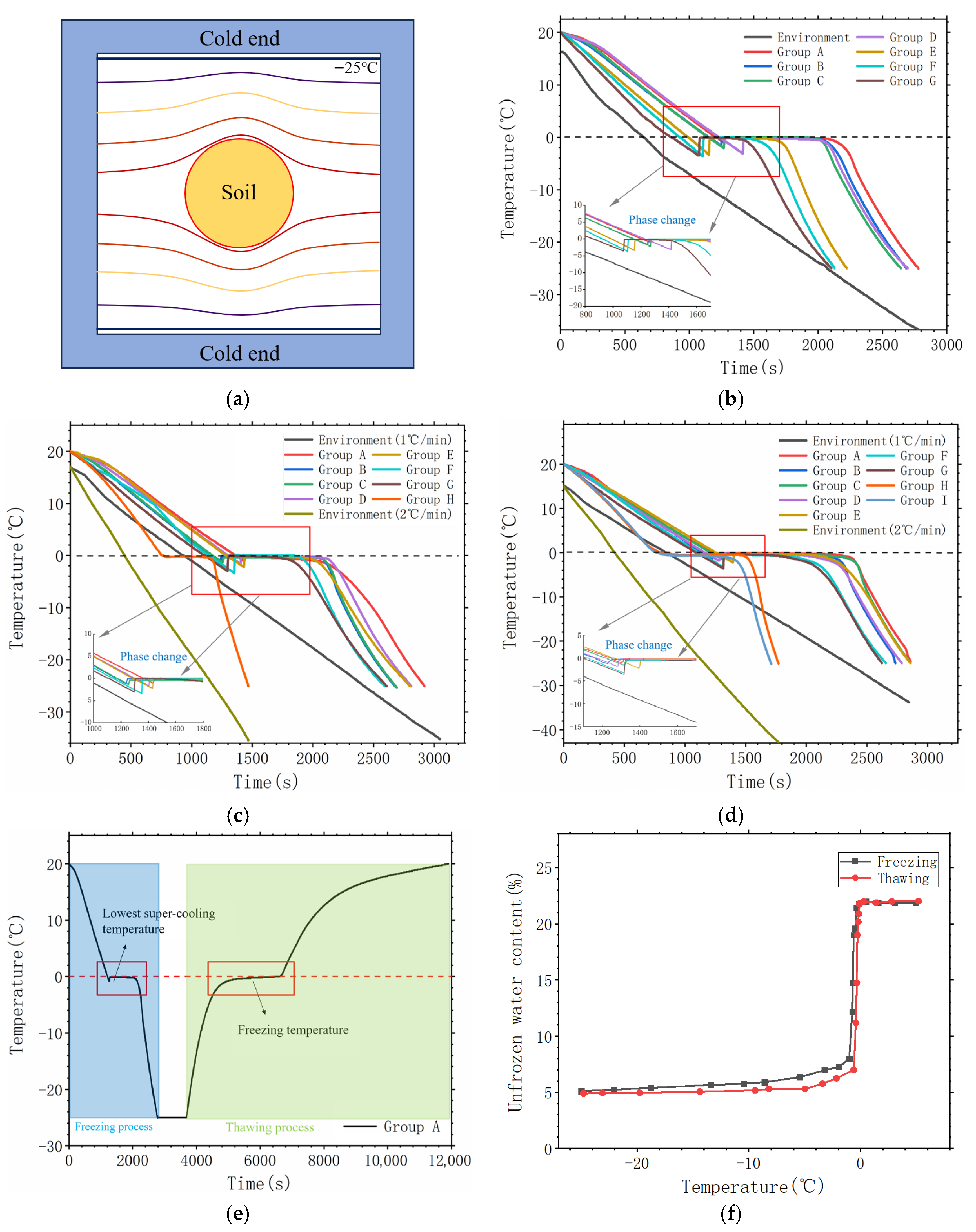
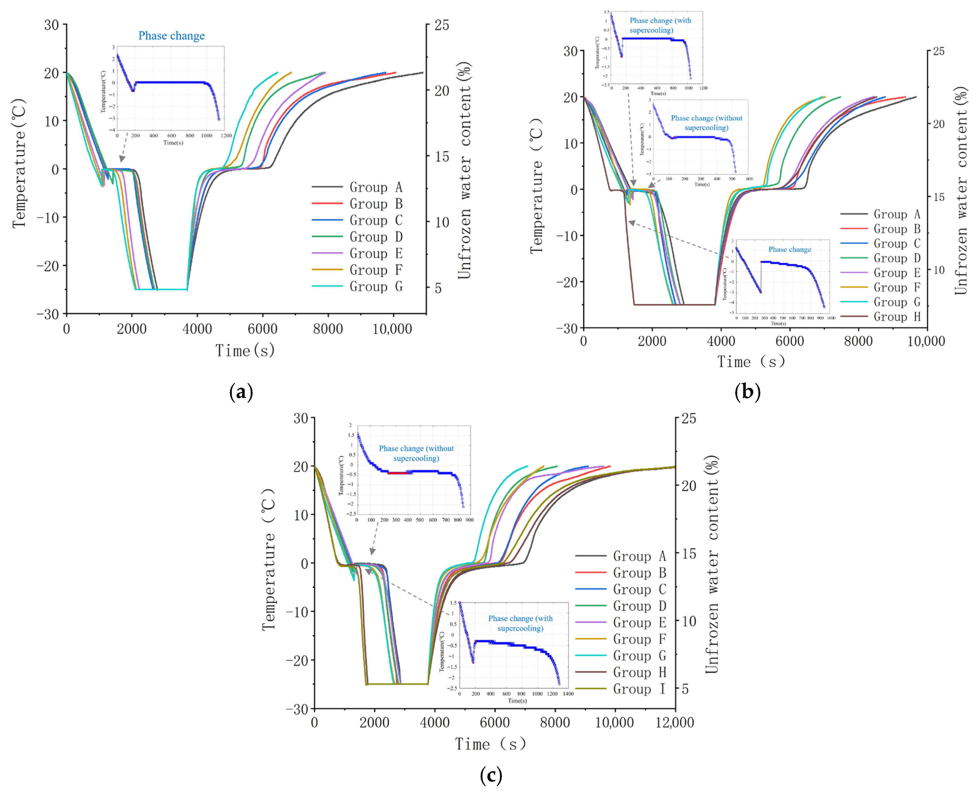
Figure 6 presents the temperature-time curves for silty soil, red clay, and mudstone under continuous cooling conditions. By comparing the ratio of environmental temperature and core temperature changes to diameter or height across sample groups, and analyzing the variation patterns of freezing temperature and supercooling temperature. Variations in sample volume across experimental groups primarily reflect differences in the temperature gradients established between the sample and its environment, as shown in Figure 6a.

$$\nabla T={\displaystyle \frac{\Delta T}{\Delta x}}$$

(5)

where ∇T is the temperature gradient, ΔT is the temperature difference, and Δx is the distance along the heat flow direction or the normal direction.

The ambient temperature was decreased at a constant rate of 1 °C/min, with the soil samples initiating cooling from a uniform initial temperature (T₀) of 25 °C. The limit temperature of supercooling for soil samples from groups A to G decreases progressively, while the supercooling duration increases progressively. During the freezing process, the samples exhibit a supercooling phenomenon. The freezing process exhibited supercooling, and the temperature at the sample center evolved through four stages: Positive temperature decline, Supercooling, Phase-change plateau, and Negative temperature decline. In Figure 6b, for the silty soil (Group G), a sudden jump occurred at 1076 s, indicating the onset of phase transformation (freezing). The temperature then rose to a freezing plateau at approximately −0.1 °C. This plateau, sustained by the release of latent heat during phase change, is characteristic of the stable freezing stage. Following the complete crystallization of free water, the stable freezing stage concludes, and the sample enters the stage of negative temperature cooling. However, the supercooling limit temperature and duration for Group G were slightly higher than those for Group F. This discrepancy is attributed to the smaller sample size in Group G, which promotes a larger temperature gradient (i.e., a greater difference between the surface and center temperatures). Furthermore, the curves suggest that a reduction in ambient temperature during the supercooling state can destabilize it, triggering rapid freezing.

Results for red clay, shown in Figure 6c: Group G exhibited slightly higher supercooling limit temperatures and longer durations compared to Group F. When the cooling rate was increased to 2 °C/min (Group H, identical in specifications to Group C), no supercooling was observed in red clay. The formation of ice crystals at the sample boundary, where the temperature drops first, can effectively suppress supercooling in the interior. In this scenario, phase change initiates at the edges while the center remains free of significant supercooling [45]. The freezing temperatures for red clay samples from the same batch were similar across different cooling rates.

For mudstone (see Figure 6d), a decrease in cooling rate from Group A to Group G corresponds to a lower supercooling limit temperature and a longer supercooling duration. In contrast, mudstone Groups H and I (specifications identical to Groups A and B, respectively) exhibited no supercooling, which is associated with a pronounced temperature gradient between the surface and interior. According to heat transfer principles, a large initial temperature difference between the sample and its environment induces a steep internal temperature gradient and a correspondingly high cooling rate. Under such rapid cooling conditions, moisture migration and aggregation within the soil are limited. Additionally, the high clay content, combined with variations in particle size and surface adsorption characteristics, results in a low overall thermal conductivity. This low thermal efficiency hinders the transfer of the latent heat of fusion and can prevent the sample from reaching the lower temperature threshold required for the nucleation of capillary water. This observation aligns with the findings of Wang et al. [46], who reported that excessively rapid cooling can delay crystallization onset and enhance the degree of supercooling.

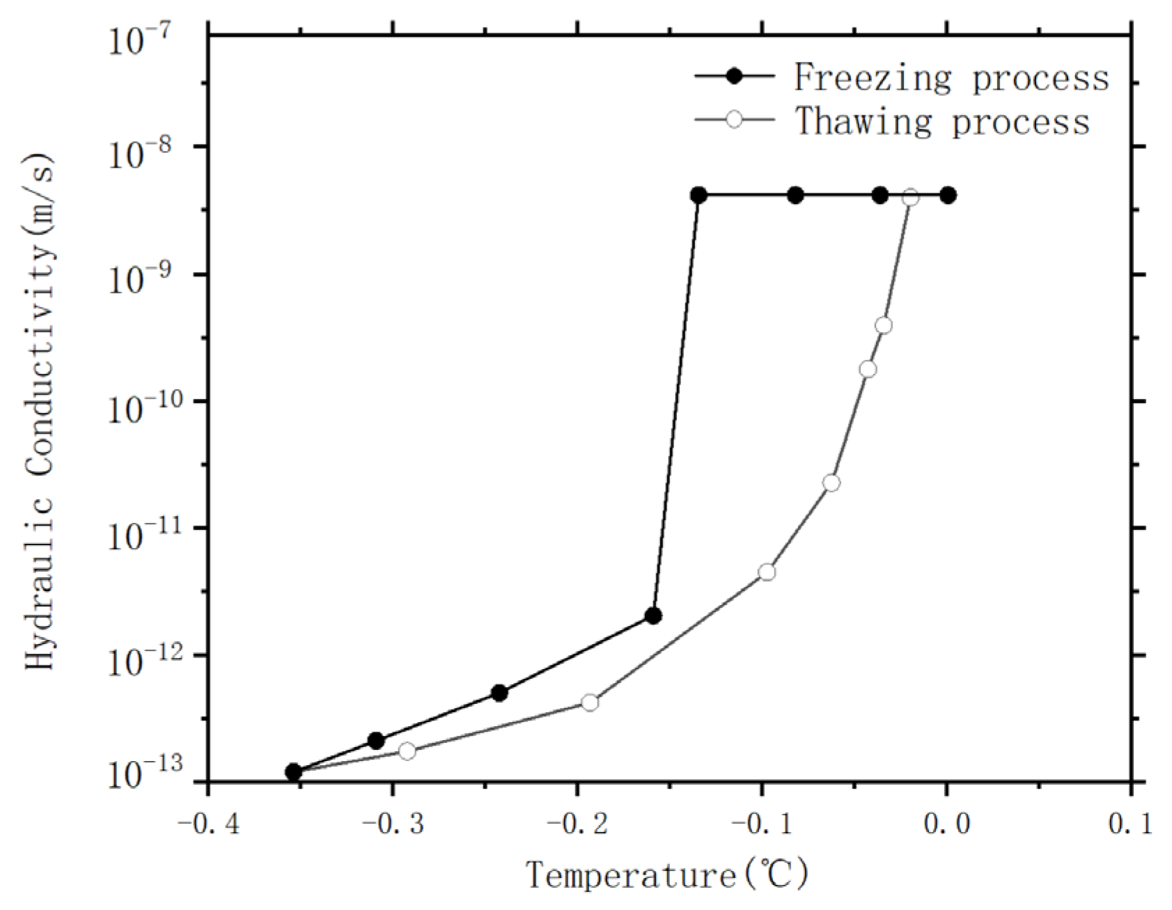
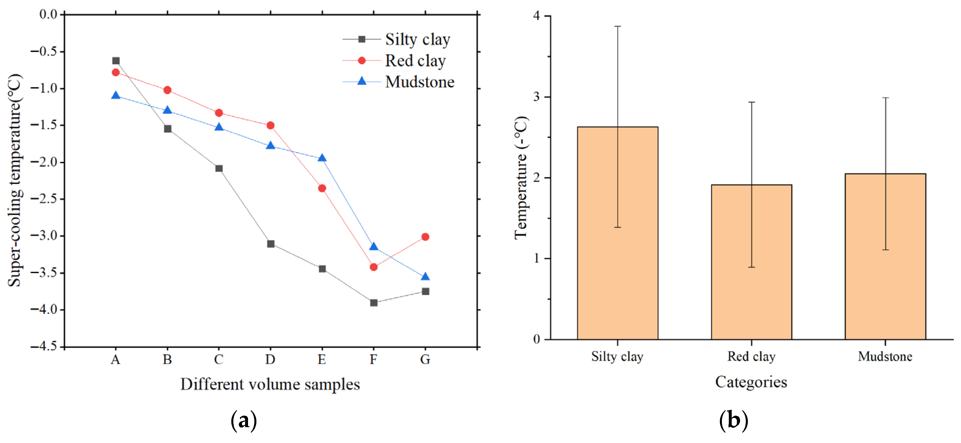
The supercooling phenomenon complicates the accurate determination of soil phase state and can consequently influence the assessment of its physical and mechanical properties. Figure 6e presents the temperature-time curve for silty clay during a freeze–thaw cycle. During continuous cooling, a supercooling limit of −0.8 °C was measured. In contrast, the warming process during thawing was gradual, exhibiting neither a sharp temperature changes analogous to the freezing plateau nor an “overheating” phenomenon. The melting phase-time curve lacks a distinct plateau at the freezing point. The variation in unfrozen water content with temperature for silty clay during a freeze–thaw cycle, as measured by nuclear magnetic resonance (NMR), is shown in Figure 6f. During freezing, a dramatic decrease in unfrozen water content occurs as the temperature reaches approximately −0.2 °C. During thawing, the unfrozen water content increases gradually, followed by a more abrupt rise at warmer temperatures. Upon warming to approximately −0.15 °C, all ice within the soil melts. At this temperature, the unfrozen water content equals the initial total water content. The inflection points on the freezing and thawing branches of the unfrozen water content curve correspond to the supercooling limit temperature and the freezing point, respectively. As shown in Figure 7, Horiguchi observed in Alaskan silt freeze–thaw experiments that the permeability coefficient exhibits a hysteretic loop during freeze–thaw cycles, analogous to the unfrozen water content curve [47]. This hysteresis is also attributed to soil supercooling effects. Figure 8 illustrates the influence of sample volume on the supercooling limit temperature. Failure to account for supercooling can lead to significant errors in estimating unfrozen water content based solely on the equilibrium water content-temperature curve, as this curve does not reflect the metastable undercooled state.

3.3. Effect of Temperature Gradient on the Freezing Temperature

The freezing temperatures of soil samples with varying dimensions were measured under continuous cooling. Representative segments of the corresponding temperature-time curves are presented in Figure 9. As shown in Figure 9a, freezing process of silty clay samples across different dimensions remained relatively stable despite variations in the imposed temperature gradient. Following the temperature jump associated with the release of latent heat (the end of supercooling), the temperature remained on a stable freezing plateau with minimal fluctuation; no stepwise decline was observed. Upon complete freezing of the free water, the samples entered the stage of sub-zero cooling. The measured freezing temperatures for silty clay predominantly fell within the range of −0.1 °C to −0.2 °C.

The freezing behavior of red clay is shown in Figure 9b. For Groups A–F, the process was stable, characterized by a well-defined freezing plateau. In contrast, Group G exhibited a stepwise temperature decline during what would typically be the stable freezing stage. This stepwise decline is attributed to a reduced temperature gradient in smaller samples (Group G), which leads to an excessively rapid cooling rate. Such rapid cooling limits moisture migration and aggregation within the soil matrix. Consequently, capillary water requires a lower ambient temperature to initiate freezing, creating the conditions for the observed stepwise cooling pattern. Although Group H samples did not exhibit a distinct supercooling state, a freezing temperature could still be inferred from the temperature plateau during phase change. Based on data from multiple groups, the statistically derived freezing temperature for red clay is approximately −0.25 °C. The freezing temperatures for red clay samples from the same batch showed little variation across different applied cooling rates, indicating that the cooling rate has a negligible effect on the freezing point.

Notably, the temperature profiles for all mudstone samples in Figure 9c are stable. When the cooling rate was increased to 2 °C/min, mudstone Groups H and I exhibited no supercooling phase. Consequently, their temperature curves lack a distinct freezing plateau and the associated temperature jump; the freezing process progressed in a stable, monotonic manner. The stable freezing plateau indicates that phase change in free water occurred at an internal sample temperature of −0.4 °C, which is therefore identified as the actual freezing temperature. In contrast, the temperature profile for mudstone Group D exhibited a stepwise decline during the (normally stable) freezing stage. This anomalous behavior is attributed to the sample’s low height-to-diameter (or aspect) ratio, which was less than 0.5. Therefore, samples with such a low aspect ratio should be avoided in future experimental designs to ensure more uniform freezing behavior. Mudstone samples F and G also display a monotonic (non-stepwise) freezing trend. This is consistent with the rapid cooling rates induced by their reduced sample volumes. Mudstone appears to be more sensitive to changes in temperature gradient (driven by volume changes) than to the gradient’s absolute magnitude, as the latter shows little influence on its freezing point. Based on the present experimental results, the freezing temperature of the tested mudstone is approximately −0.4 °C.

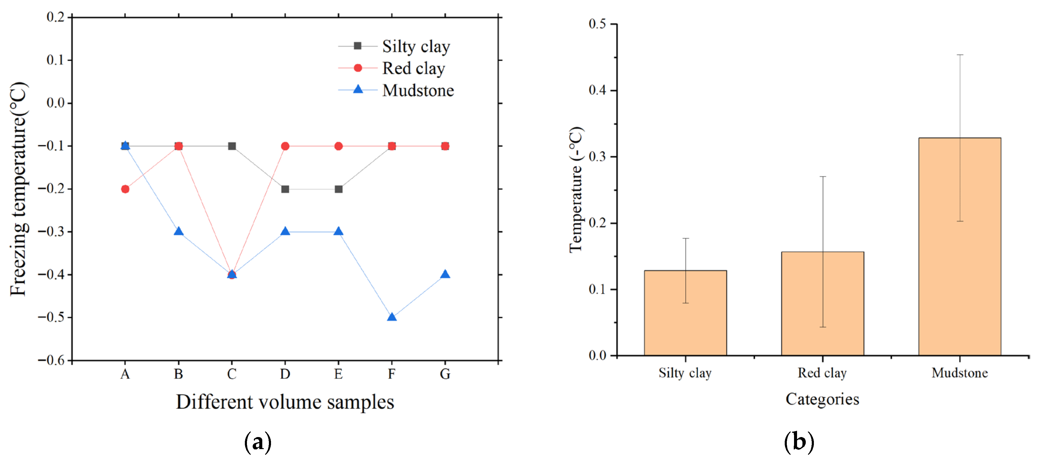
Soil water exists in various forms, primarily as free water, capillary water, and adsorbed water. Analysis of the temperature–time curves for the three soil types with varying dimensions allows for the construction of a relationship between freezing temperature and sample volume, as presented in Figure 10. The freezing temperature shows no obvious correlation with variations in the temperature gradient. In contrast, the supercooling limit temperature exhibits a clear inverse relationship with the gradient, decreasing as the gradient diminishes. Despite minor fluctuations, the overall trend is relatively gentle and displays a good linear fit.

3.4. Unfrozen Water Content Under Different Temperature Gradient Conditions

Nuclear magnetic resonance (NMR) is a powerful technique for characterizing porous media. It yields critical information regarding pore structure, including porosity, pore size distribution, permeability, and fluid saturation. In smaller pores, the higher surface-to-volume (S/V) ratio leads to more frequent collisions between hydrogen nuclei and pore walls. This accelerates energy dissipation, resulting in a shorter transverse relaxation time [48]. Consequently, the proportionality between the transverse relaxation time (T₂) and pore radius is leveraged in NMR measurements to infer the pore structure and connectivity within soil samples.

The transverse relaxation time, T₂, is described by the following relationship:

$${\displaystyle \frac{1}{T_2}}={\displaystyle \frac{1}{T_{2,\mathrm{f}}}}+{\displaystyle \frac{1}{T_{2,\mathrm{s}}}}+{\displaystyle \frac{1}{T_{2,\mathrm{d}}}}={\displaystyle \frac{1}{T_{2,\mathrm{f}}}}+{\rho }_2{\left({\displaystyle \frac{S}{V}}\right)}_{\mathrm{p}}+{\displaystyle \frac{D{\left(\gamma G{T}_E\right)}^2}{12}}$$

(6)

where T_2,f is the bulk relaxation time of the pore fluid, governed by its intrinsic properties; T_2,s is the surface relaxation time, dependent on the surface relaxivity (ρ₂) and the pore surface-area-to-volume ratio (S/V); and T_2,d is the diffusion relaxation time, influenced by the diffusion coefficient (D), the applied magnetic field gradient (G), the gyromagnetic ratio (γ), and the echo time (T_E).

For the analyzed soil samples, the contributions of T_2,f and T_2,d are negligible. Consequently, the observed transverse relaxation time (T₂) is dominated by the surface relaxation mechanism (T_2,s). Based on this simplification, the relationship between the pore size distribution and the transverse relaxation time (T₂) for the tested samples is derived from Equation (6) as follows:

$${\displaystyle \frac{1}{T_2}}={\rho }_2\left({\displaystyle \frac{S}{V}}\right)$$

(7)

where ρ₂ is the surface relaxivity (m·s⁻¹), a material-specific constant; and (S/V) is the pore surface-area-to-volume ratio (m). For idealized geometries, S/V equals 3/R for a spherical pore model and 2/R for a cylindrical pore model, where R is the pore radius.

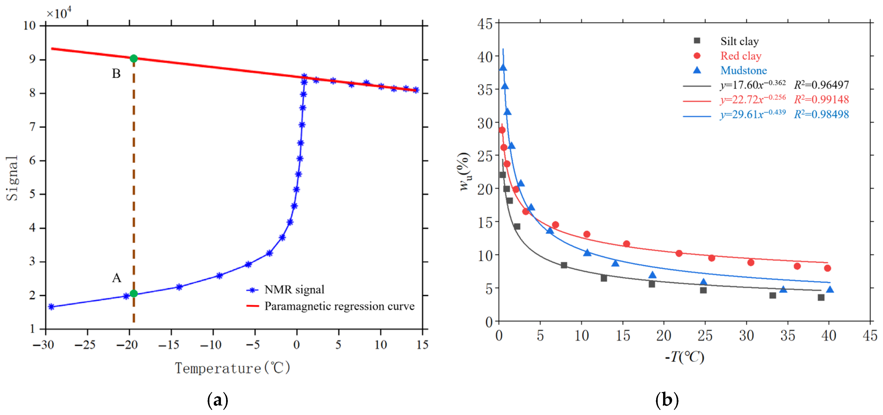
Above 0 °C, the NMR signal intensity from pore water exhibits a linear relationship with temperature. A linear regression line is therefore fitted to the data within this positive temperature range. When the temperature falls below 0 °C, a portion of the free pore water undergoes freezing. The signal from solid ice is not detectable by conventional NMR. Consequently, the total observed NMR signal begins to decrease. The rate of this decrease gradually diminishes until a stable residual signal level is reached. The unfrozen water content in the soil samples was quantified based on the reduction in the NMR signal intensity [49]. By extrapolating the linear regression line (established from the positive temperature data) into the sub-zero temperature range (see Figure 11a), the frozen water content at a given sub-zero temperature can be calculated as the difference between the extrapolated total water signal and the measured NMR signal. This relationship is expressed by the following equation:

$$w_u=A{\theta }^{-B}$$

(8)

where w_u is unfrozen water content (%), θ is the absolute value of the sub-zero temperature (°C), and A and B are soil-specific empirical coefficients. The functional relationship was validated by fitting the model to experimental data obtained from three distinct soil types (see Figure 11b). The close agreement between the model and the data demonstrates the reliability of the NMR technique for quantifying unfrozen water content.

4. Numerical Simulation

4.1. Modeling Process

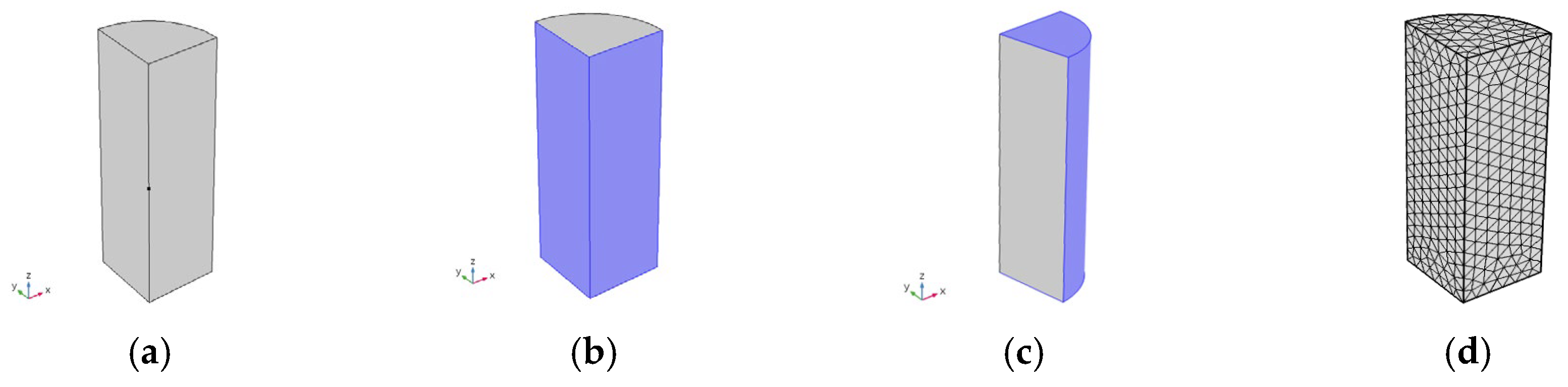
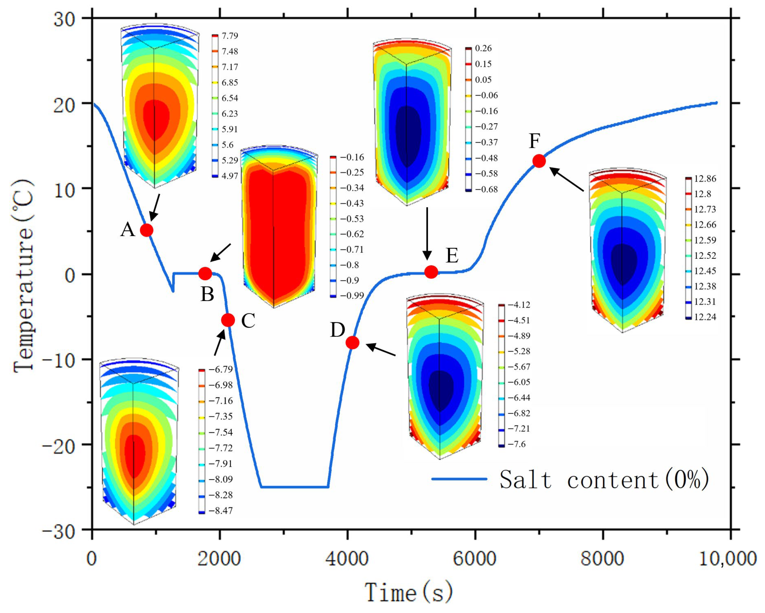
Numerical simulation programs incorporating thermal-hydraulic coupling serve as an effective means for investigating the hydraulic and thermal characteristics of unsaturated soils under freeze–thaw cycling conditions [50]. Quarter-symmetric models of the freeze–thaw process were developed using COMSOL Multiphysics^® software 6.1. The simulations considered a silty clay sample with a diameter (D) of 20 mm and a height (H) of 30 mm, at three different salt contents: 0%, 1.5%, and 2.5%. The model geometry and boundary conditions are illustrated in Figure 12, and the thermal properties are listed in

Table 3. Thermal parameters used in the numerical model.

Heat Transfer Coefficient, h (W/(m2•K))	Latent Heat of Water (kJ/kg)	Specific Heat of the Soil (kJ/(kg•K))	Specific Heat of Water (kJ/(kg•K))	Specific Heat of Ice (kJ/(kg•K))	Heat Conductivity Coefficient (W/(m•K))
					Before Freeze	After Freeze
12.0–15.0	336.0	0.77	4.2	2.0	1.924	1.389

. Convective heat flux boundaries were applied to the top, bottom, and cylindrical outer surfaces of the sample. The temperature dependence of the unfrozen water content was defined via an interpolation function. The external ambient temperature was set to 20 °C.

4.2. Data Analysis

Figure 13 shows the temporal evolution of temperature isosurfaces during freezing. The model exhibits a layered freezing front propagating from the exterior to the interior. Accordingly, the lowest temperatures occur at the outer surface, while the highest temperatures are maintained at the sample center. The simulation was initialized with a uniform temperature of 20 °C throughout the model. After 600 s of freezing, the radial temperature difference between the outer surface and the center was 2.82 °C. During this initial stage, the overall sample temperature decreased rapidly. By 1200 s, this radial temperature difference had reduced to 0.83 °C, indicating a more uniform temperature distribution within the sample. At this stage, the overall cooling rate increased. The evolution of the radial temperature difference was non-monotonic: it initially increased, then decreased, followed by another increase, before finally diminishing as the overall temperature stabilized. The magnitude of the radial temperature difference serves as an indicator of the freezing front propagation speed. In the later stages of freezing, the cooling rate decreased significantly.

The numerical simulation results indicate that during freezing, the sample temperature decreases with time, exhibiting a gradient from the cooler exterior to the warmer interior. Similar to the experimental observations, the freezing process can be delineated into three distinct stages:

Stage I: Positive Temperature Decline. In this initial stage before reaching 0 °C, the sample temperature declines rapidly. The cooling rate is high, and the temperature-time profile is approximately linear. Stage II: Freezing Plateau. Upon reaching the freezing point (approximately −0.2 °C), pore water begins to freeze, releasing latent heat. This release largely offsets the heat loss to the environment, resulting in a near-constant temperature—a characteristic freezing plateau—despite ongoing phase change. Stage III: Sub-zero Cooling. After the majority of free water has frozen, the rate of latent heat release diminishes and can no longer balance the environmental heat loss. Consequently, the soil temperature resumes declining below the freezing point.

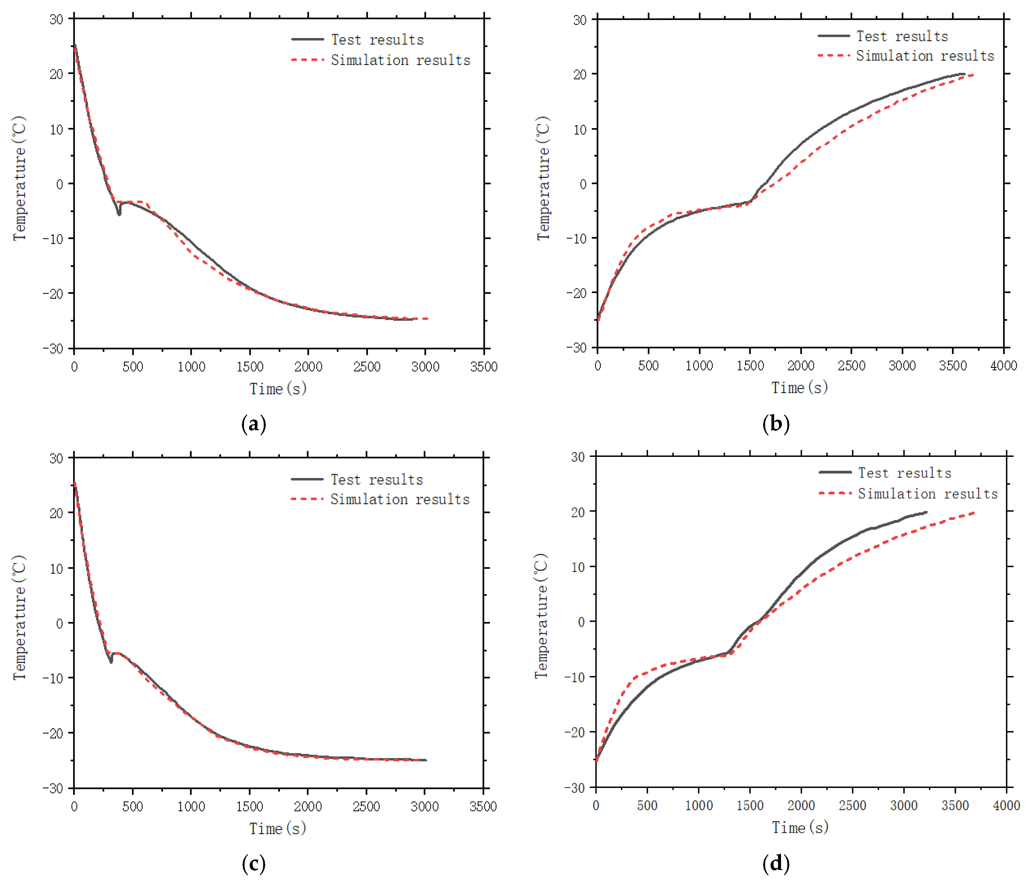
The supercooling phenomenon observed in experiments was transient and resulted in no significant ice formation. As its effect on the overall unfrozen water content calculation was negligible, it was omitted from the numerical model. A comparison of experimental and simulation results (Figure 14) shows good agreement in the overall trend. For the salt-free sample, both datasets exhibit a reduction in the cooling rate upon entering the freezing plateau, which minimizes the discrepancy between test and simulation.

During the thawing process, melting progresses from the exterior towards the interior. Consequently, the highest temperatures are at the outer surface, and the lowest temperatures remain at the core. The model was initialized at a uniform temperature of −25 °C. After 600 s of thawing, a radial temperature difference of 3.48 °C was measured between the surface and the core. This initial thawing phase was characterized by rapid warming. By 1200 s, the radial temperature difference had decreased to 0.94 °C, and the warming rate slowed compared to the initial phase, indicating a more uniform temperature distribution. At 1800 s and 2400 s, the radial temperature differences were 1.28 °C and 2.82 °C, respectively. The evolution of this difference during thawing was non-monotonic, initially increasing, then decreasing, before ultimately diminishing as the system approached thermal equilibrium. The magnitude of the radial temperature difference correlates with the thawing front propagation speed: a larger difference corresponds to faster thawing. The same simulation methodology was applied to samples with salt contents of 1.5% and 2.5%. The characteristic unfrozen water content curve for each salinity was incorporated into the model to simulate their freeze–thaw behavior.

Comparison of the simulated and experimental results leads to the following conclusions: (1) Overall Trend Agreement: The simulation captures the overall trend of the experimental temperature evolution. Any deviations in the warming/cooling rates are likely attributable to minor ambient temperature fluctuations in the lab, whereas a constant 20 °C boundary condition was used in the simulation. (2) Model Validation and Applicability: The consistency between the numerical and experimental results validates the simulation approach. This demonstrates the potential of the method for simulating soil freeze–thaw processes over a broader range of conditions.

5. Conclusions

To improve the efficiency of determining the supercooling and freezing temperatures of frozen soil compared to traditional thermocouple methods, this study proposes a continuous cooling test method with controllable boundary conditions. The research findings systematically reveal the intrinsic mechanisms underlying the supercooling and freezing processes in unsaturated frozen soil. Its conceptual innovation and broad significance are primarily manifested in the following four aspects:

(1)

Analysis of temperature–time curves for various soil types and sample volumes under continuous cooling revealed key supercooling characteristics, including the limit temperature and duration. The results demonstrate that a smaller temperature gradient between the sample and its environment leads to a lower supercooling limit temperature and a longer supercooling duration. Conversely, an excessively high cooling rate, driven by a large initial temperature difference, can suppress supercooling at the sample core due to dominant boundary effects. The temperature difference between the sample surface and the ambient environment is thus a key factor governing the supercooling state.

(2)

The initial freezing temperatures of silty clay, red clay, and mudstone across a range of sample dimensions were measured at a constant water content. It was found that neither the imposed temperature gradient nor the cooling rate significantly influenced the measured freezing point. The freezing process of silty clay was stable. Mudstone exhibited greater sensitivity to changes in temperature gradient induced by variations in sample volume.

(3)

During freezing, a layered freezing front propagated from the exterior to the interior. The overall cooling rate was initially high and then decreased until thermal equilibrium was approached upon completion of phase change. During thawing, melting progressed inward from the surface. The warming rate varied non-monotonically: initially rapid, then slower, before increasing again in the final stages. The close agreement between experimental observations and numerical simulations validates both the reliability of the numerical model and the accuracy of the input parameters.

(4)

The proposed continuous cooling method significantly reduces the time required to determine the soil supercooling limit temperature and initial freezing point. Theoretically, this method enables the measurement of a standard sample set within approximately one hour, representing a substantial time saving compared to traditional step-wise cooling or constant-temperature methods.

These findings demonstrate that regulating the cooling rate and the temperature difference between the sample center and its boundary allows for effective control over the supercooling and phase change behavior of frozen soil. This offers critical experimental evidence for predicting the in situ freezing progression and frost heave potential of frozen soil in cold regions. However, this study has limitations: The findings from controlled laboratory cooling experiments may not fully represent complex field conditions, which involve heterogeneous thermal boundaries, inherent soil structure, and long-term thermal fluctuations. It has not sufficiently considered the coupled effects of multiple physical fields such as salinity, pore water chemistry, and stress states. Future research should prioritize several directions. First, developing in situ monitoring methods for rapid cooling processes is essential. Integrating multi-parameter sensing (e.g., thermal, electrical, acoustic) can elucidate the spatiotemporal heterogeneity of soil freezing under natural thermal gradients. Additionally, the mechanisms through which salinity, contaminants, and soil-ice interface phenomena affect supercooling temperature and unfrozen water transport require systematic investigation to establish a coupled chemo-thermal theoretical model. Furthermore, a multiscale numerical simulation platform spanning from microscopic pores to macroscopic engineering scales is needed to predict the complete process from ice nucleation to frost heave development. Finally, systematic comparative experiments across diverse soil types and environmental conditions are recommended to quantify the sensitivity of freezing behavior to key factors. This will provide more generalized practical guidance for the design and risk mitigation of cold-regions infrastructure.

References

1. Wu, Y.D.; Wang, Y.J.; Hu, L.M. A unified soil freezing characteristic curve model incorporating supercooling, capillarity, adsorption, and solute effects. J. Hydrol. 2025, 662, 133899. [Google Scholar] [CrossRef]
2. Wang, X.W.; Gao, Y.C.; Hou, J.G.; Yang, J.H.; Smits, K.; He, H.L. Machine learning facilitates connections between soil thermal conductivity, soil water content, and soil matric potential. J. Hydrol. 2024, 633, 130950. [Google Scholar] [CrossRef]
3. Li, S.X.; Cheng, G.D.; Guo, D.X. The Future Thermal Regime of Numerical Simulating Permafrost on Qinghai-Xizang (Tibet) Plateau, China, under Climate Warming. Sci. China Ser. D Earth Sci. 1996, 39, 434–441. [Google Scholar]
4. Shan, W.; Wu, J.; Guo, Y. Establishment and Experimental Validation of a Temperature–Unfrozen Water Content Model for Frozen Soil. Water 2025, 17, 846. [Google Scholar] [CrossRef]
5. Ke, X.M.; Wang, W.; Niu, F.J.; Gao, Z.Y. Investigating soil properties and their effects on freeze-thaw processes in a thermokarst lake region of Qinghai-Tibet Plateau, China. Eng. Geol. 2024, 342, 107734. [Google Scholar] [CrossRef]
6. Wu, Q.B.; Li, X.; Li, W.J. The Response Model of Permafrost along the Qinghai—Tibetan Highway under Climate Change. J. Glaciol. Geocryol. 2001, 23, 1–6. [Google Scholar]
7. Liu, H.; Huang, S.B.; Xie, C.; Tian, B.S.; Chen, M.; Chang, Z.Q. Monitoring Roadbed Stability in Permafrost Area of Qinghai-Tibet Railway by MT-InSAR Technology. Land 2023, 12, 474. [Google Scholar] [CrossRef]
8. Cui, G. Determination of Freezing Temperature and Thickness of Frozen Wall in Wet Soil with Thick Topsoil. J. China Univ. Min. Technol. 1997, 3, 3–6. [Google Scholar]
9. Zhao, G.; Tao, X.X.; Liu, B. Experimental Research on Water Migration in Remolded Soil during Freezing and Thawing Process. J. Cent. South Univ. (Sci. Technol.) 2009, 40, 519–525. [Google Scholar]
10. Liu, Z.Y.; Liu, J.K.; Li, X.; Fang, J.H. Experimental Study on Freezing Point and Deformation Characteristics of Unsaturated Silty Clay Subjected to Freeze-thaw Cycles. Chin. J. Geotech. Eng. 2017, 39, 1381–1387. [Google Scholar] [CrossRef]
11. Morgenstern, N.R.; Tsytovich, N.A.; Swinzow, G.K. The mechanics of Frozen Ground. Am. J. Sci. 1976, 276, 7. [Google Scholar] [CrossRef]
12. Tice, A.; Anderson, D.; Banin, A. The Prediction of Unfrozen Water Contents in Frozen Soils from Liquid Limit Determinations. In Symposium on Frost Action on Roads (Paris: Transportation Research Board); Cold Regions Research Laboratory: Hanover, NH, USA, 1973; pp. 329–344. [Google Scholar]
13. Wei, P.C.; Yin, Z.Y.; Yao, C.; Ren, Z.F.; Zheng, Y.Y.; Ma, W. Atomistic origin of montmorillonite clay subjected to freeze-thaw hysteresis. J. Rock Mech. Geotech. Eng. 2024, 17, 5989–6006. [Google Scholar] [CrossRef]
14. Tomasz, K. A Semi-empirical Model for Phase Composition of Water in Clay-water Systems. Cold Reg. Sci. Technol. 2007, 49, 226–236. [Google Scholar] [CrossRef]
15. Wu, Y.D.; Wang, Y.J.; Hu, L.M. Molecular insights into the freezing process of water on the basal surface of muscovite mica. Appl. Clay Sci. 2024, 256, 107431. [Google Scholar] [CrossRef]
16. Yoshikawa, K.; Overduin, P. Comparing Unfrozen Water Content Measurements of Frozen Soil using Recently Developed Commercial Sensors. Cold Reg. Sci. Technol. 2005, 42, 250–256. [Google Scholar] [CrossRef]
17. Wan, X. Experimental Study on the Feezing Temperatures of Saline Silty Soils. Permafr. Periglac. Process. 2015, 26, 175–187. [Google Scholar] [CrossRef]
18. Dash, J. The Physics of Permeated Ice and its Geophysical Consequences. Rev. Mod. Phys. 2006, 78, 695–741. [Google Scholar] [CrossRef]
19. Wan, X.S.; Liu, E.L.; Qiu, E.X. Study on ice nucleation temperature and water freezing in saline soils. Permafr. Periglac. Process. 2021, 32, 119–138. [Google Scholar] [CrossRef]
20. Liu, Z. Freezing Points of Wet Soil and its Measurement. J. China Univ. Min. Technol. 1986, 3, 24–31. [Google Scholar]
21. Yao, Y.F.; Cheng, H.; Lin, J.; Ji, J.C.; Zhang, Z.M. Fuzzy random sensitivity analysis model for reliability of freezing shaft lining structure in deep alluvium. J. Min. Saf. Eng. 2022, 39, 107–117. [Google Scholar] [CrossRef]
22. Cui, G. The Study on Freezing Point of Wet Sand under Loads. J. Glaciol. Geocryol. 1994, 16, 320–326. [Google Scholar] [CrossRef]
23. Li, Y. A Study on Freezing Point of Wet Clay under Loading. J. Glaciol. Geocryol. 1996, 18, 43–46. [Google Scholar] [CrossRef]
24. Leng, Y. Experimental Research on the Unfrozen Water Content of Frozen Soils by Calorimetry. Rock Soil Mech. 2010, 31, 3758–3764. [Google Scholar]
25. Zhou, Y.Y.; Zhang, J.J.; Niu, J.Y.; Chen, F.Y.; Zhang, Q.; Yan, S.J.; Hu, J.L. Application of ultrasonic-induced nucleation technology in the freezing point test. Chin. J. Rock Mech. Eng. 2021, 40, 3052–3062. [Google Scholar] [CrossRef]
26. Li, D. The Experiment and Theoretical Research on a New Test Method to Measure Unfrozen Water Content in Frozen Soil. Doctoral Thesis, China University of Mining and Technology, Beijing, China, 2011; pp. 97–99. [Google Scholar]
27. Ying, S.; Zhou, F.X.; Wen, T. Study on Characteristic Temperatures of Cooling Saline Soil. Pol. J. Environ. Stud. 2021, 30, 1893–1901. [Google Scholar] [CrossRef]
28. Zhou, J. Unified Soil Freezing Characteristic for Variably-saturated Saline Soils. Water Resour. Res. 2020, 56, 1–14. [Google Scholar] [CrossRef]
29. Xu, X. Factors Affecting Water Migration in Frozen Soil. CRREL Rep. 1987, 9, 16. [Google Scholar]
30. Chen, W.; Wan, W.; He, H.; Liao, D.X.; Liu, J. Temperature Field Distribution and Numerical Simulation of Improved Freezing Scheme for Shafts in Loose and Soft Stratum. Rock Mech. Rock Eng. 2024, 57, 2695–2725. [Google Scholar] [CrossRef]
31. Liu, J.L.; Xu, Q.; Li, P.L.; Pu, C.H.; Zhao, K.Y.; Peng, D.L.; Lei, M.Y. Determination of Nuclear Magnetic Resonance T2 Cutoff in Remoulded Loess by the Freezing Point. Eur. J. Soil Sci. 2023, 74, e13406. [Google Scholar] [CrossRef]
32. Bing, H.; Ma, W. Laboratory Investigation of the Freezing Point of Saline Soil. Cold Reg. Sci. Technol. 2011, 67, 79–88. [Google Scholar] [CrossRef]
33. Kozlowski, T. Some Factors Affecting Supercooling and the Equilibrium Freezing Point in Soil-water Systems. Cold Reg. Sci. Technol. 2009, 59, 25–33. [Google Scholar] [CrossRef]
34. Kozlowski, T. A Simple Method of Obtaining the Soil Freezing Point Depression, the Unfrozen Water Content, and the Pore Size Distribution Curves from the DSC Peak Maximum Temperature. Cold Reg. Sci. Technol. 2016, 122, 18–25. [Google Scholar] [CrossRef]
35. Low, P.F.; Anderson, D.M.; Hoekstra, P. Some Thermodynamic Relationships for Soils at or below the Freezing Foint: 1. Freezing Point Depression and Heat Capacity. Water Resour. Res. 1968, 4, 379–394. [Google Scholar] [CrossRef]
36. Hu, G.J.; Zhao, L.; Li, R.; Wu, X.D.; Wu, T.H.; Zou, D.F.; Zhu, X.F.; Chen, J.; Su, Y.Q.; Hao, J.M.; et al. Dynamics of the Freeze–thaw Front of Active Layer on the Qinghai-Tibet Plateau. Geoderma 2023, 430, 116353. [Google Scholar] [CrossRef]
37. Tounsi, H.; Rouabhi, A.; Tijani, M.; Guérin, F. Thermo-hydro-mechanical Modeling of Artificial Ground Freezing: Application in Mining Engineering. Rock Mech. Rock Eng. 2019, 52, 3889–3907. [Google Scholar] [CrossRef]
38. Cengel, Y.A. Heat Transfer; Higher Education Press: Beijing, China, 2007; pp. 143–144. [Google Scholar]
39. Liu, B.; He, Y.Q.; Han, Y.H.; Li, T.; Li, D.Y.; Gao, R. An improved model assessing variation characteristics of pore structure of sandy soil thawing from extremely low temperature using NMR technique. Cold Reg. Sci. Technol. 2023, 205, 103717. [Google Scholar] [CrossRef]
40. Xu, X. Experimental Research on Water Migration in Frozen Soil; Beijing Science Press: Beijing, China, 1991. [Google Scholar]
41. Luo, H.L.; Teng, J.D.; Zhang, S.; Sheng, D.C. Study on the relationship between unfrozen water content and electrical conductivity in frozen soils. Chin. J. Rock Mech. Eng. 2021, 40, 1068–1079. [Google Scholar] [CrossRef]
42. GB/T50123; Standard for Geotechnical Test Methods. China Planning Press: Beijing, China, 2019; pp. 168–175.
43. Liu, B.; Li, D.Y. A Simple Test Method to Measure Unfrozen Water Content in Clay-water Systems. Cold Reg. Sci. Technol. 2012, 78, 97–106. [Google Scholar] [CrossRef]
44. Liu, B.; Li, D.Y. Test Study of Unfrozen Water Content in Artificial Frozen Silt. Chin. J. Rock Mech. Eng. 2012, 31, 3696–3702. [Google Scholar]
45. Zhou, J.Z.; Tan, L.; Wei, C.F.; Wei, H.Z. Experimental Research on Freezing Temperature and Super-cooling Temperature of Soil. Rock Soil Mech. 2015, 36, 777–785. [Google Scholar] [CrossRef]
46. Wang, C.; Li, K.Y.; Cai, H.H.; Wu, Y.M.; Lin, Z.K.; Li, S.Y. Study of Supercooling Phenomena in Soil-water Systems Based on Nucleation Theory: Quantifying Supercooling Degree. Water Resour. Res. 2023, 59, e2023WR035935. [Google Scholar] [CrossRef]
47. Horiguchi, K. Hydraulic conductivity functions of frozen materials. In Proceedings of 4th International Conference on Permafrost; National Academy Press: Washington, DC, USA, 1983; pp. 504–508. [Google Scholar]
48. Coates, G.; Xiao, L.; Prammer, M. NMR Logging: Principles & Applications; Halliburton Energy Services: Houston, TX, USA, 1999. [Google Scholar]
49. Yan, W.; Sun, J.; Sun, Y.; Golsanami, N. A Robust NMR Method to Measure Porosity of Low Porosity Rocks. Microporous Mesoporous Mater. 2018, 269, 113–117. [Google Scholar] [CrossRef]
50. Soltanpour, S.; Foriero, A. Numerical Modelling of Coupled Thermal–Hydraulic–Mechanical Processes in Unsaturated Soils During Freezing and Thawing. Water 2025, 17, 677. [Google Scholar] [CrossRef]
Figure 1. Standard freezing process. (Points 1, 2 and 3 respectively represent the positive temperature point, the beginning point of phase change and the end point of the freezing process.)
Applsci 16 02140 g001
Figure 2. Freezing process with supercooling. (Points 1, 2, 3, 4, and 5 respectively represent the positive temperature point, the beginning point of supercooling, the lowest supercooling temperature point, the end point of supercooling, and the end point of the freezing process.)
Applsci 16 02140 g002
Figure 3. Experimental setup.
Applsci 16 02140 g003
Figure 4. Temperature–time curves of distilled water and environment.
Applsci 16 02140 g004
Figure 5. Particle size distribution of the silty clay.
Applsci 16 02140 g005
Figure 6. Unfrozen volumetric water content-time curves. (a) Temperature Gradient Distribution Map. (b) Supercooling limit temperature–temperature gradient curve for silty clay. (c) Supercooling limit temperature–temperature gradient curve for red clay. (d) Supercooling limit temperature–temperature gradient curve for mudstone. (e) Freeze–thaw cycle curve. (f) Unfrozen water content–time curves.
Applsci 16 02140 g006
Figure 7. Hydraulic conductivity–temperature curves of Fairbanks silt during freezing and thawing.
Applsci 16 02140 g007
Figure 8. Diagram of supercooling limit temperature in soil particles: (a) Influence of sample volume on supercooling limit temperature. (b) Supercooling limit temperature error bar.
Applsci 16 02140 g008
Figure 9. Freezing temperature-temperature gradient curve. (a) Silty clay. (b) Red clay. (c) Mudstone.
Applsci 16 02140 g009
Figure 10. Diagram of freezing temperature in soil particles: (a) Freezing temperature–temperature gradient curve. (b) Freezing temperature error bar.
Applsci 16 02140 g010
Figure 11. Relationship between unfrozen water content and temperature. (a) Calculation of unfrozen water content. (b) Unfrozen water content–temperature curve.
Applsci 16 02140 g011
Figure 12. Numerical simulation model. (a) Quarter-symmetry specimen geometry. (b) Symmetry boundary. (c) Convective heat flux boundary. (d) Computational mesh.
Applsci 16 02140 g012
Figure 13. Results of numerical simulation.
Applsci 16 02140 g013
Figure 14. Comparison of simulation and experimental results. (a) Freezing process: Salt content 1.5%. (b) Thawing process: Salt content 1.5%. (c) Freezing process: Salt content 2.5%. (d) Thawing process: Salt content 2.5%.
Applsci 16 02140 g014