A Geological Modeling Workflow for Shale Reservoirs: A Case Study of the F2 Member in the Qintong Sag

Abstract

Shale reservoirs provide critical storage space for unconventional oil and gas, yet their frequent vertical facies alternations and complex spatial architectures make it difficult for conventional two-point geostatistical methods to reproduce thin interbedding and reservoir-scale continuity. Multiple-point geostatistics can incorporate structural information through training images (TIs), but practical 3D shale modeling is often hindered by the limited availability of representative 3D TIs. Using the F2 Member in the Qintong Sag, Subei Basin, eastern China, as a case study, we propose a hierarchical 2D-to-3D geological modeling workflow that combines mixed-point geostatistical simulation (MIXSIM) for generating vertical 2D facies sections and a sequential 2D simulation strategy with conditioning data (s2Dcd) for propagating section-based patterns into 3D space under hard well constraints. In the workflow, vertical sections serve as TI carriers to explicitly capture bedding-scale alternations, while well data are imposed as hard conditioning information during 3D simulation. Quantitative evaluation is performed in terms of (i) conditioning-data consistency, (ii) vertical facies-transition statistics quantified by transition counts and Markov transition probability matrices, (iii) global facies proportions summarized as the mean of 10 realizations, and (iv) connectivity characterized by connected geobody analysis. The realizations honor the conditioning data exactly, reproduce vertical transition behavior with a transition-matrix discrepancy of $D_{\mathrm{M}\mathrm{A}\mathrm{E}}=0.0396$, and maintain global facies proportions close to well-based estimates with a maximum deviation of 2.36%. These results demonstrate that the proposed MIXSIM–s2Dcd workflow provides a practical solution for well-data-driven, high-resolution 3D shale facies modeling when 3D training images are unavailable.

1. Introduction

Shale reservoirs, as critical storage spaces for unconventional hydrocarbons, exhibit stratified architectures and facies stacking patterns that govern the dominant scales and spatial expressions of reservoir heterogeneity [1,2,3,4,5]. In the development of unconventional oil and gas fields, geological modeling provides the foundation for reservoir evaluation, development planning, and uncertainty assessment [6,7,8,9]. However, shale reservoirs are commonly characterized by frequent vertical facies alternations, the coexistence of thin interbeds and laterally continuous bedding, and, in many cases, sparse well control and limited 3D constraints [10,11,12,13]. These factors jointly make practical 3D structural modeling challenging. Conventional two-point geostatistical methods rely on second-order statistics to quantify spatial correlation. They offer clear physical interpretability and operational simplicity for representing global-scale, stationary correlation structures, yet they have limited capability in describing bedding assemblages, nonlinear connectivity, and multiscale superposition. Multiple-point geostatistics (MPS), by contrast, incorporates higher-order structural information through training images (TIs), thereby providing geologically more consistent reconstructions of continuity and morphology [14,15,16,17]. Nevertheless, 3D MPS modeling depends strongly on high-quality 3D TIs, which are often unavailable or difficult to construct in data-limited field settings, directly restricting its practical deployment.

In parallel with geostatistical approaches, deep-learning methods have recently gained momentum in reservoir and facies modeling. In particular, deep generative models (e.g., GAN-based and diffusion-based frameworks) have been explored for conditional facies simulation, aiming to learn complex spatial patterns from training realizations and generate multiple plausible 3D outcomes under conditioning constraints [18]. Meanwhile, deep learning has also been used to assist geostatistical workflows by accelerating or enriching prior pattern information, such as constructing training-image libraries or providing data-driven priors for subsequent modeling [19]. Despite these advances, many AI-driven workflows still require abundant, representative training data and careful treatment of conditioning and uncertainty, which can be non-trivial in shale settings where well control is sparse and 3D constraints are limited. Therefore, a practical modeling strategy that remains interpretable and operational under data-limited conditions is still needed to complement modern AI-based approaches.

A common strategy in existing studies is to generate 3D TIs using object-based or process-based modeling methods so that depositional architectures and connectivity features are embedded in the TI itself [20]. However, the range of structures that such methods can represent is relatively limited [21], and the results depend heavily on predefined geometric rules and parameterizations. For example, Fluvsim is primarily tailored to fluvial architectural modeling [22]; when the target shifts to non-fluvial systems or reservoirs with more complex structural patterns, developing separate sets of geometric equations and parameter rules for diverse morphologies becomes labor-intensive and does not necessarily ensure that the resulting TIs adequately cover the structural variability observed in reality. Because 3D TIs are often difficult to obtain directly in field applications or may fail to meet representativeness requirements, increasing attention has been paid to workflows that drive 3D simulations directly from 2D sectional information [21,23,24]. In such approaches, interwell sections, interpreted seismic sections, or outcrop sections are used as 2D TIs or structural constraints, and 3D modeling is achieved by propagating 2D patterns into 3D space, thereby balancing feasibility and geological plausibility under limited data conditions.

Motivated by this perspective, this study takes the shale reservoir of the F2 Member in the Qintong Sag as a case study and develops a 3D modeling workflow tailored for data-limited settings. First, under well control, vertical 2D facies sections are constructed using the mixed-point geostatistical simulation algorithm (MIXSIM) [25] to encode vertical bedding assemblages and facies-belt variations. These vertical 2D sections are then used as TIs, with well data imposed as hard conditioning information, and a sequential 2D simulation strategy with conditioning data (s2Dcd) [23] is employed to propagate and extend the 2D patterns into 3D space. In this way, 3D structural modeling of shale reservoirs can be accomplished without relying on 3D TIs.

2. Materials and Methods

2.1. Geological Setting and Data

2.1.1. Study Area of the F2 Member

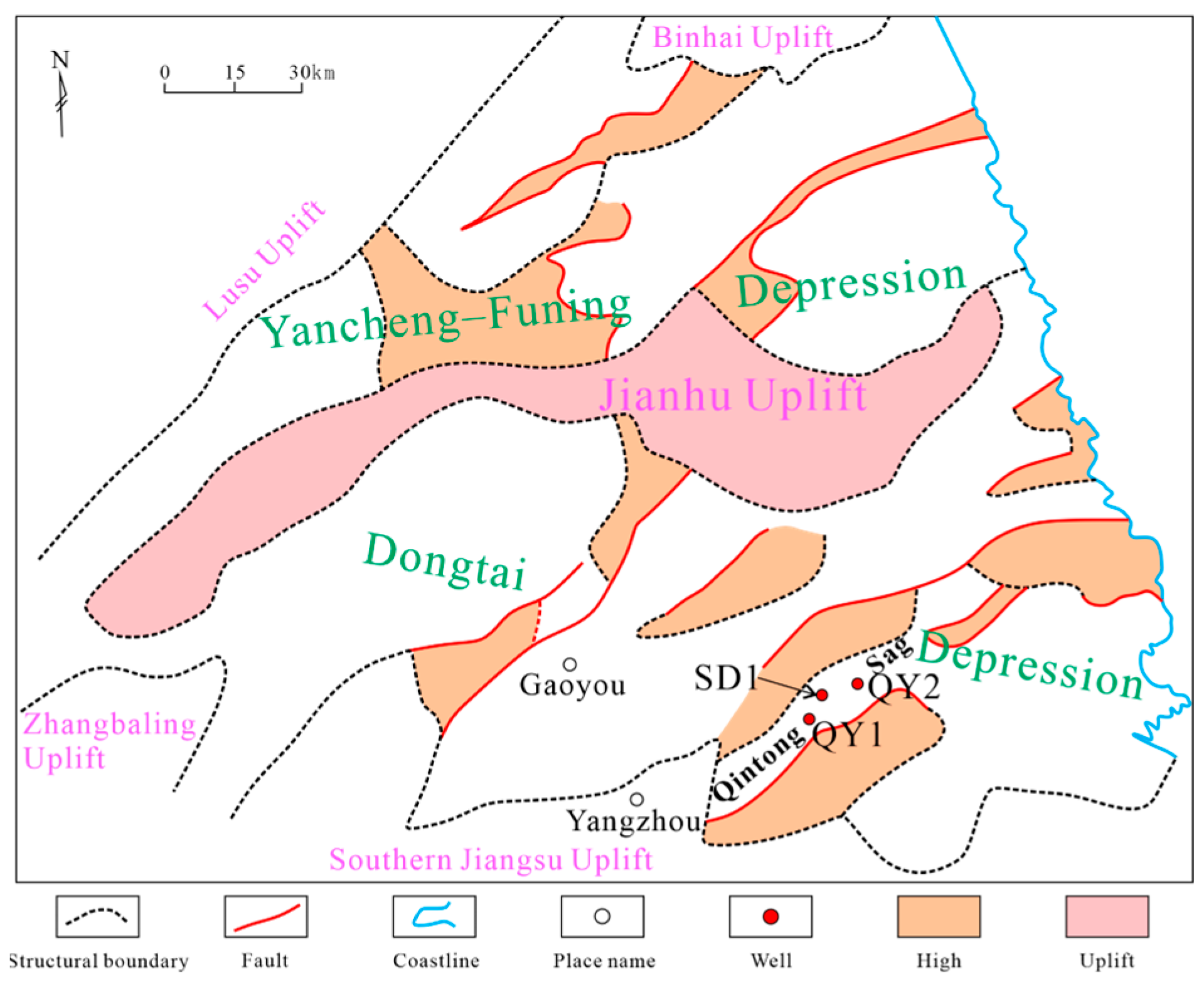
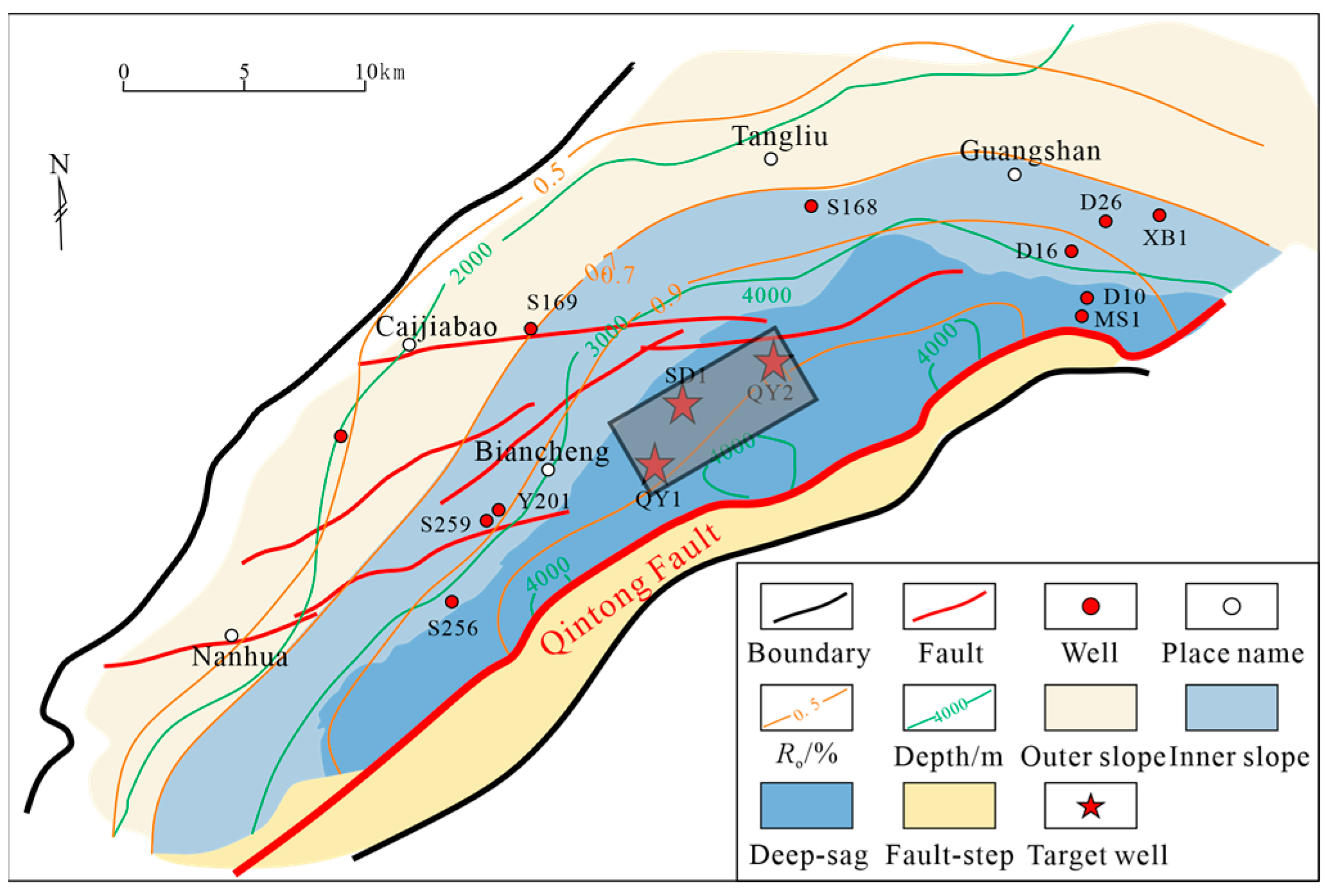
The Qintong Sag is located within the Yancheng–Funing Depression of the Subei Basin in eastern China and represents a key target for the development of deep-sag source rocks and shale-oil exploration in the basin [26] (Figure 1). The Subei Basin developed on the Paleozoic folded basement of the Yangtze Platform and is characterized by an overall “one uplift–two depressions” structural framework, comprising the Jianhu Uplift, the Yancheng–Funing Depression, and the Dongtai Depression. The Qintong Sag lies within the Yancheng–Funing Depression and forms a deep depocenter in the basin-scale sedimentary–tectonic architecture [27,28] (Figure 2). The target interval of this study is the F2 Member, deposited predominantly in a lacustrine setting. During F2 deposition, water depth generally increased from west to east, transitioning from shallow-lake to semi-deep–deep lake conditions, and forming a shale-dominated sedimentary succession with a thickness of approximately 250–450 m. The F2 Member is typified by mixed-lithology laminated shale, in which argillaceous laminae and felsic laminae commonly alternate vertically. Frequent variations in bedding assemblages and facies stacking make this member a key interval for shale-oil generation and enrichment in the study area. Based on sedimentary cycles, lithologic associations, and petrophysical responses, the F2 Member can be further subdivided into five sub-members. Among them, F2-1 and F2-2 exhibit relatively stronger gas-logging anomalies, indicating vertical heterogeneity and zonation of favorable intervals. Three representative wells (QY1, QY2, and SD1) were selected for facies interpretation. These wells are located, respectively, in the central deep-sag zone, the transitional area between the gentle-slope belt and the deep-sag zone, and a relatively uplifted position along the western margin of the sag. Together, they capture the major structural–sedimentary positional differences within the sag and provide the well control for subsequent 2D section construction and 3D modeling.

2.1.2. Well Data and Facies Classification Criteria

This chapter uses the F2 interval of the Qintong Sag as a case study to validate the proposed shale modeling workflow, namely “vertical-section construction followed by 2D-to-3D extension”. The study area is discretized using a regular 3D grid with a size of $73\times 31\times 1351$, corresponding to grid spacings of $\mathsf{\Delta }x=\mathsf{\Delta }y=100 \mathrm{m}$ and $\mathsf{\Delta }z=1 \mathrm{m}$. The model covers an area of approximately $7.3 \mathrm{k}\mathrm{m}\times 3.1 \mathrm{k}\mathrm{m}$ in plan view and about $1.35 \mathrm{k}\mathrm{m}$ in the vertical direction. Three wells (QY1, QY2, and SD1) are selected as sources of hard conditioning data. The well-based facies interpretations are consistently coded as a discrete facies variable $M\in \{1,\dots ,K\}$ with $K=6$. The six facies types are defined by jointly considering organic-matter richness (organic-rich vs. organic-lean) and structural style (bedded, laminated, or massive), as summarized in

Table 1. Facies classification for the F2 interval ($K=6$).

Facies Name	Code	Organic Richness Criterion	Bedding-Style Criterion	Well-Based Proportion
Organic-lean laminated mudstone	1	TOC < 2.0 wt.%	Laminated	34.79%
Organic-lean bedded mudstone	2	TOC < 2.0 wt.%	Bedded	36.98%
Organic-lean massive mudstone	3	TOC < 2.0 wt.%	Massive	2.95%
Organic-rich laminated mudstone	4	TOC ≥ 2.0 wt.%	Laminated	4.18%
Organic-rich bedded mudstone	5	TOC ≥ 2.0 wt.%	Bedded	17.91%
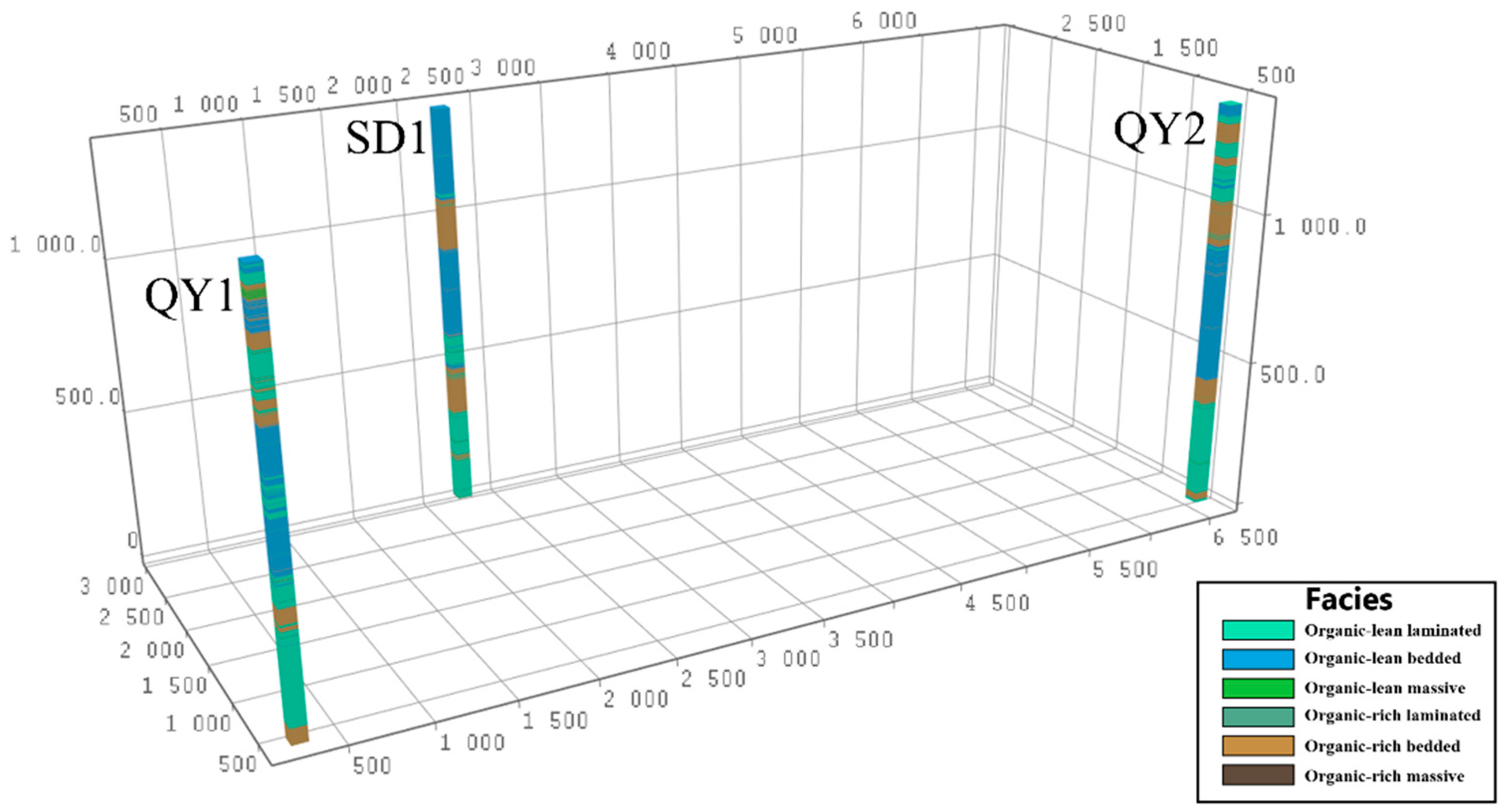
Organic-rich massive mudstone	6	TOC ≥ 2.0 wt.%	Massive	3.17%

. Well trajectories are mapped into the grid system, and cells intersected by the wells are assigned the corresponding facies values and kept fixed during subsequent simulations, as shown in Figure 3, whereas cells not constrained by well data constitute the target domain for stochastic simulation.

2.2. Modeling Workflow

2.2.1. Modeling Strategy and Overall Workflow

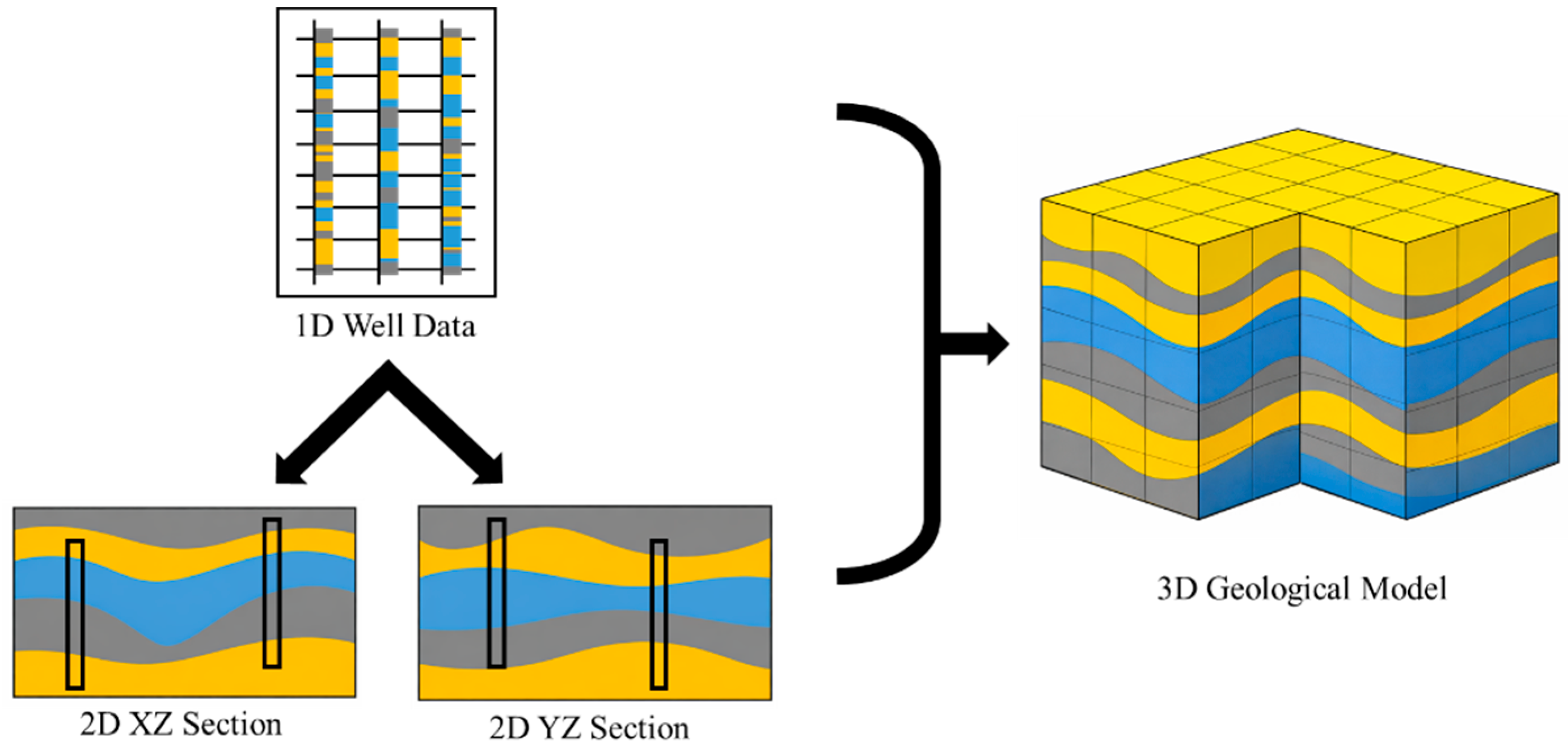
In the workflow proposed in this study, a two-step strategy is implemented, as shown in Figure 4. Under hard well constraints, vertical 2D facies sections are first constructed to capture bedding assemblages and stacking relationships and are treated as training-image (TI) carriers. These 2D sections are then used as TIs, with the well data imposed as hard conditioning information, to propagate sectional patterns into 3D and construct the 3D facies model.

2.2.2. Data Preparation

As shown in

Table 2. Functions of different data types within the 3D geological modeling workflow.

Data Type	Dimensionality	Acquisition	Role in the Modeling Workflow
Well data	1D	Drilling and well-logging data	Used to construct vertical 2D sections; incorporated as hard conditioning data during the 2D-to-3D modeling stage
XZ vertical section	2D	Generated from well data using multiple-point geostatistical modeling methods	Used as a 2D training image, providing vertical structural samples in the XZ direction
YZ vertical section	2D	Generated from well data using multiple-point geostatistical modeling methods	Used as a 2D training image, providing vertical structural samples in the YZ direction
3D simulation grid	3D	Discretized as a regular 3D grid over the study area	Acts as the spatial domain for 2D-to-3D reconstruction

, different data types play complementary roles in the proposed workflow. A set of representative wells in the study area was selected as sample wells for facies classification and 2D section construction. The facies sequences of each well were consistently coded by integrating log responses, core observations, and existing interpretation results, yielding a discrete facies variable $M\in \{1,\dots ,K\}$, where $K$denotes the number of facies categories. To ensure consistency with the subsequent 3D simulation grid, the well data were resampled according to the vertical discretization of the target grid, such that the wellbore facies sequence aligns with the number of vertical grid layers $n_z$. Meanwhile, well trajectories were mapped onto the regular 3D grid $\left(n_x,n_y,n_z\right)$. Facies values at well locations were written into the simulation domain as hard conditioning data and kept fixed during simulation. Grid cells not covered by well data remained unassigned and constituted the target region for stochastic simulation [23,25].

To ensure consistency between 2D section construction and 3D modeling, a unified facies coding scheme and grid resolution were adopted for both the 2D sections and the 3D grid, allowing the section results to be seamlessly used as training images in subsequent modeling. Section lines were arranged along well-to-well directions. Under the constraints of well distribution and geological understanding, typical interwell sections that best capture the major sedimentary–structural features of the study area were preferentially selected, so as to improve the representativeness of the 2D training images in terms of vertical bedding assemblages and facies stacking patterns.

2.2.3. Conceptual Basis for Vertical Section Modeling

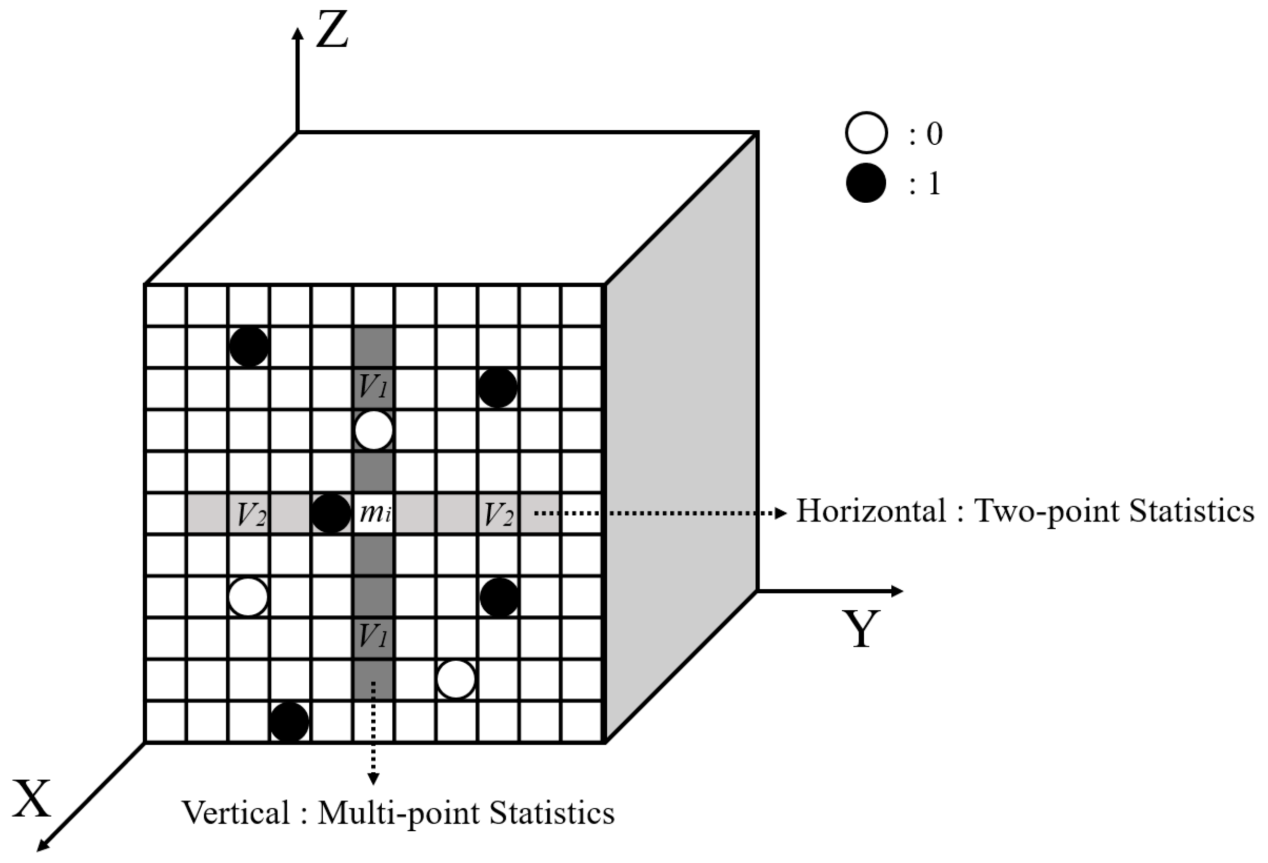
The objective of modeling vertical 2D sections is to generate, under hard conditioning to well data, facies architectures that reproduce the key characteristics of the F2 shale interval—namely, frequent bedding alternations and pronounced lamina stacking—while avoiding the oversmoothing that often arises when relying solely on two-point statistics. To this end, we adopt the mixed-point geostatistical simulation method (MIXSIM) proposed by Cordua et al. [25] to construct vertical 2D facies sections in the XZ and YZ planes, as illustrated in Figure 5. This procedure is not a simple interwell interpolation; instead, it performs geostatistical simulation by explicitly accounting for directional differences in information support within a section.

When constructing an XZ or YZ section, the well data are first inserted into the 2D section grid as hard conditioning data. Along the vertical direction, the 1D facies sequences derived from wells are used as TIs to provide multiple-point statistical constraints, thereby controlling stratigraphic stacking and facies-transition patterns associated with bedding assemblages. In contrast, information support in the horizontal direction within the section is relatively weak due to well spacing and sparse well density. Accordingly, two-point statistics are employed as the primary constraint to control the overall correlation scale and lateral continuity in interwell regions. By coupling vertical multiple-point constraints with horizontal two-point constraints within the same vertical section, the simulated sections inherit the well-implied vertical structural patterns while maintaining statistically plausible continuity between wells, providing stable structural inputs for propagating 2D training-image patterns into 3D space in subsequent modeling.

Specifically, given the above characteristics of information support, MIXSIM operates within a sequential simulation framework and constructs local conditional probability distributions provided by two-point and multiple-point statistics, respectively. Let $m_i$ denote the $i$-th target node to be simulated within a section. The conditional probability distribution inferred from multiple-point statistics (e.g., SNESIM) under the vertical neighborhood $V_1$ is denoted as $p_{\mathrm{M}\mathrm{P}}(m_i\mid V_1)$, whereas the conditional probability distribution inferred from two-point statistics (e.g., SISIM) under the horizontal neighborhood $V_2$ is denoted as $p_{\mathrm{T}\mathrm{P}}(m_i\mid V_2)$. In MIXSIM, these two conditional distributions are combined at the same simulation location, and the resulting joint distribution can be expressed as:

$$p\left(m_i∣V_1,V_2\right)={\displaystyle \frac{p_{\mathrm{M}\mathrm{P}}\left(m_i∣V_1\right)p_{TP}\left(m_i∣V_2\right)}{p\left(m_i\right)}}$$

(1)

where $p\left(m_i\right)$ is the prior marginal distribution of node $m_i$, which is used to normalize the combined probability distribution.

Through this probability-fusion mechanism, as defined in Equation (1), the vertical sections can faithfully inherit the bedding-stacking patterns implied by the well data in the vertical direction, while maintaining lateral continuity governed by two-point statistics in the horizontal direction. The resulting XZ and YZ sections honor the observations exactly at well locations and exhibit geologically plausible structural extensions in interwell areas. It should be emphasized that the objective of the vertical-section stage is not to recover a single, deterministic “true section”, but rather to generate a set of statistically plausible 2D vertical structural descriptions. These sections are subsequently used as 2D training images to drive the 2D-to-3D structural modeling in the following workflow.

2.2.4. 3D Model Construction Using 2D Training Images

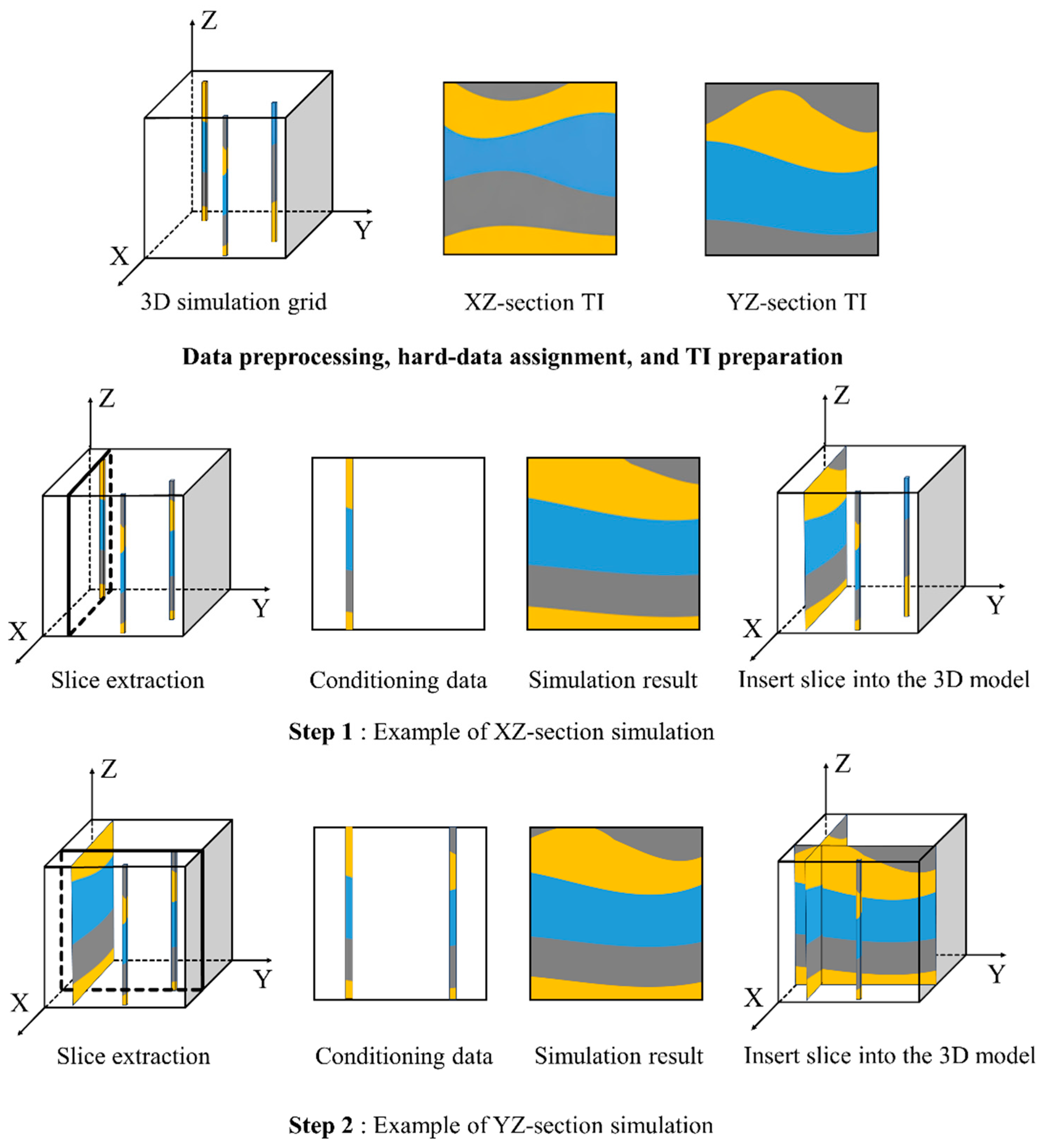
After obtaining the vertical 2D sections in the XZ and YZ directions, the central task of 3D modeling for the F2 shale interval can be reformulated as follows: how to jointly exploit these two 2D sections in a 3D domain, under hard conditioning to well data, to construct a model that reproduces the vertical bedding assemblages and lamina-stacking characteristics of the shale reservoir. Unlike conventional point-by-point 3D simulation, we adopt a 2D-to-3D modeling strategy inspired by the s2Dcd concept, as illustrated in Figure 6. Its key feature is that the 3D model is not generated directly through node-wise simulation driven by a 3D training image; instead, 2D multiple-point simulations are performed sequentially on a series of slices along different directions, and the simulated results from each directional set of slices are progressively transferred and fused as conditioning information to form the 3D structure [23]. This strategy is well aligned with the problem addressed in this study: the most critical structural information in the F2 shale interval is expressed by vertical bedding rhythms and facies stacking patterns, which, under the available data conditions, are reliably constrained mainly by well observations. Therefore, using vertical sections as training images and propagating them into 3D through slice-based simulation better matches the data characteristics of shale reservoirs, namely strong vertical constraints and relatively weak lateral constraints.

Within this framework, the 3D grid is decomposed into a series of 2D slices lying in the XZ and YZ planes. For each set of slices, the simulation follows the basic principle of 2D multiple-point statistics: the vertical section in the corresponding direction is used as the training image, and 2D structural simulation is performed within the slice so that the result inherits, in a statistical sense, the vertical bedding assemblages and transition rhythms expressed by the training image. Because the XZ and YZ sections capture vertical structural characteristics along different directions, they jointly serve as training images in the s2Dcd framework, enabling the 3D model to assimilate vertical structural information from multiple orientations during construction.

It should be emphasized that slices along different directions in the s2Dcd method are not simulated independently. Once the simulation of a slice in one direction is completed, its result is incorporated as conditioning information in the subsequent simulation of slices in other directions, thereby progressively establishing consistency among structural features across orientations in 3D space. This iterative “slice–condition–re-slice” procedure ensures that the model not only preserves training-image-like structures within individual slices, but also forms coherent bedding extensions and stacking relationships at the 3D scale, avoiding structural inconsistencies that would arise from simply superimposing results from different directions.

During the 2D-to-3D modeling process, well data participate continuously in the slice simulations as hard conditioning data. For slices intersecting the well trajectories, the 2D simulation must honor the observed well facies values exactly at the corresponding locations. For slices that do not directly pass through wells, well information is incorporated indirectly through the conditioning data provided by previously simulated slices. In this manner, well control is maintained throughout the iterative slice-updating process, ensuring that the final 3D model matches the observations strictly at well locations

Overall, the slice-based 2D simulation and conditioning-transfer mechanism of s2Dcd provides a practical route to construct 3D shale geological models in the absence of 3D training images. In the proposed workflow, this method naturally connects with the preceding strategy for vertical-section construction, allowing the 2D structural descriptions in both the XZ and YZ directions to work collaboratively within a unified framework and ultimately yielding a 3D model that captures shale bedding characteristics while exactly honoring well control.

2.2.5. Parameter Settings and Implementation Details

To ensure reproducibility, the key parameter settings used in both steps of the proposed workflow—vertical 2D section construction using MIXSIM and 3D facies modeling using the s2Dcd strategy—are summarized in

Table 3. Parameter settings for MIXSIM-based construction of well-constrained vertical 2D facies sections.

Parameter	Value	Description
Simulation grid size	(73, 1351), (31, 1351)	2D simulation grid dimensions
Number of 1D training images	3	Number of input well logs used
Conditioning enabled	1	Hard conditioning is activated
Covariance type	2	Type of covaraince function used, 2 = spherical
$\mathrm{Template}\mathrm{size}\mathrm{in}x$	30	$\mathrm{Template}\mathrm{extent}\mathrm{size}\mathrm{along}x$ direction
$\mathrm{Template}\mathrm{size}\mathrm{in}y$	150	$\mathrm{Template}\mathrm{extent}\mathrm{size}\mathrm{along}y$ direction
Range parameter	100	Range parameter used
Random seed	42	Random seed parameters

and

Table 4. Parameter settings for s2Dcd 3D facies simulation using vertical 2D sections as TI carriers.

Parameter	Value	Description
Simulation grid size	(73, 31, 1351)	3D simulation grid dimensions
Distance type	Proportion of mismatching nodes	Categorical distance used
Section types (TIs)	XZ and YZ	Two orthogonal vertical sections used as 2D training-image carriers
Max number of neighbors	50	Maximum number of conditioning nodes retained in the pattern
Acceptance threshold	0.02	Maximum allowed pattern distance
Max scan fraction	0.5	Maximum fraction of the TI scanned for simulating each cell
Random seed	42	Random seed parameters

. In this study, the workflow was implemented based on the published implementations provided in the original publications of MIXSIM and s2Dcd [23,25]. We used their released code as the computational backbone and adapted it to the present case by harmonizing the grid discretization and facies coding with the F2 dataset and enforcing hard well conditioning throughout the simulations. All simulations reported in this paper were generated using the parameter values listed in Table 3 and Table 4, so that the results can be reproduced under the same discretization and conditioning setup.

3. Results

3.1. Results of Vertical 2D Section Modeling

In the geological modeling of the F2 shale interval, vertical bedding assemblages and facies-stacking rhythms constitute the key structural information controlling reservoir heterogeneity, and well data provide the most direct and reliable observations of these vertical features. Based on the MIXSIM method described in Section 3.3, vertical 2D facies sections were constructed in both the XZ and YZ directions.

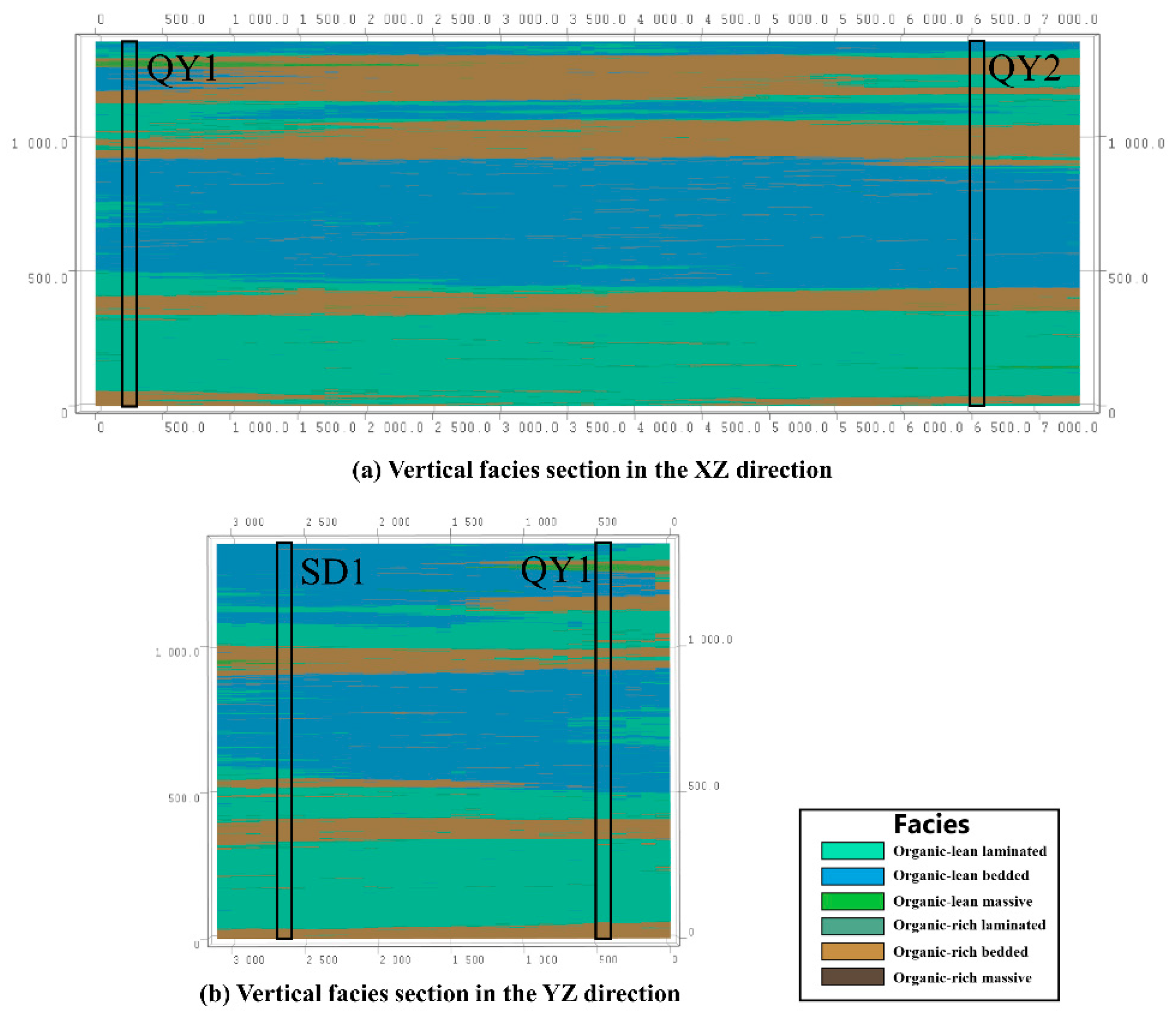
The results show that the generated XZ and YZ vertical sections honor the input facies sequences exactly at the well locations, with no violation of hard conditioning data (Figure 7). In the interwell areas, the sections effectively extend the bedding-assemblage characteristics revealed by the wells, manifested by continuous vertical stacking and frequent alternations of laminated/bedded facies, while massive facies tend to occur in relatively concentrated intervals. Overall, the simulated structures are consistent with the general geological understanding of the F2 shale interval, namely well-developed lamination and rapid vertical variability. Facies transitions exhibit clear stacking relationships on the sections, avoiding both the oversmoothing commonly produced by simple two-point interpolation and the unconstrained, fragmented patterns that may arise in interwell regions.

3.2. Results of 3D Geological Modeling

After obtaining the vertical 2D sections in the XZ and YZ directions, a 3D facies model of the F2 shale interval was constructed using the s2Dcd method described in Section 2.2.4. The key of this step is to progressively propagate the bedding assemblages and facies-stacking rhythms encoded in the vertical sections into 3D space and to form an overall consistent 3D architecture under hard conditioning. The regular grid model is taken as the simulation domain, and well data are imposed as hard constraints and kept fixed throughout the simulation, ensuring that the model matches the interpreted observations exactly at well locations.

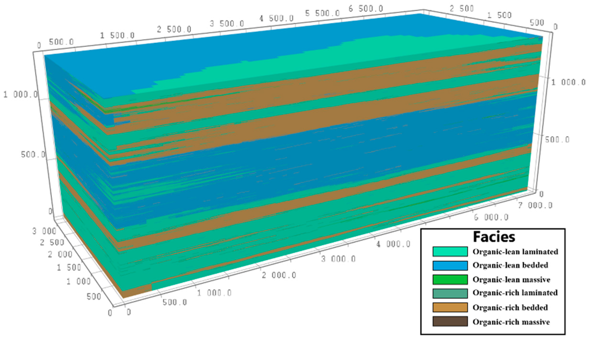
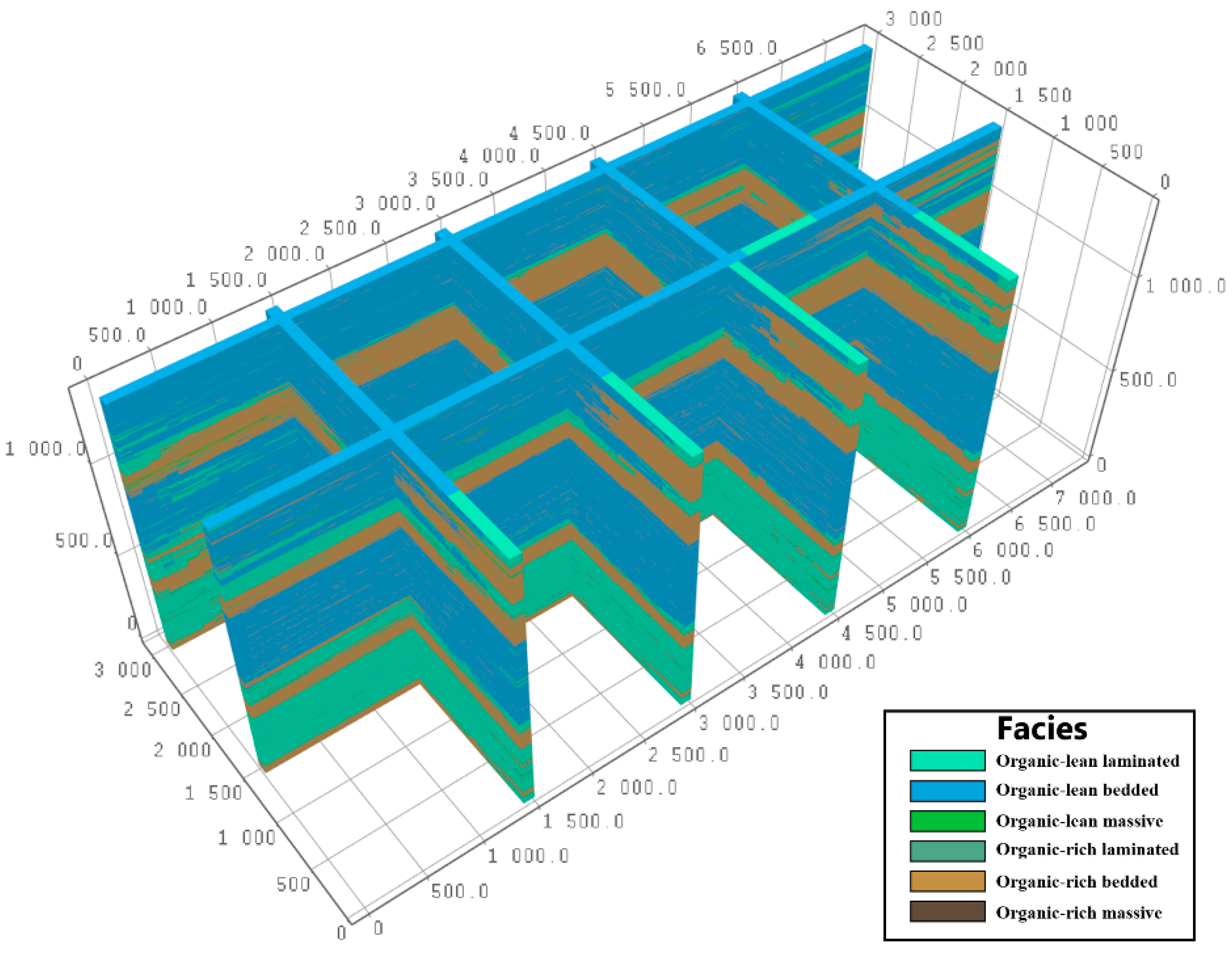
Figure 8 presents an overall view of the 3D facies model, in which the wells remain fixed as hard conditioning data. To illustrate the propagation of 2D structures into 3D space, several representative slices in the XZ and YZ directions are extracted and displayed (Figure 9). The slice comparisons show that the model achieves smooth transitions near the intersections of slices from different directions, and that conditioning information from previously simulated slices is effectively transferred to subsequent slices, enabling the structural patterns expressed by the 2D sections to propagate coherently throughout the 3D domain.

3.3. Statistical Validation

To assess the reliability and interpretability of the 3D modeling results under data-limited conditions, we conduct a quantitative evaluation based on four complementary aspects: (i) conditioning-data consistency, (ii) vertical facies-transition statistics, (iii) global facies proportions, and (iv) connectivity characteristics of the target facies. It should be noted that only three wells are available in the study area, and all of them are required to construct the orthogonal vertical sections that act as pattern carriers in the proposed workflow; therefore, a conventional blind-well test is not feasible without altering the workflow configuration. Consequently, the evaluation herein focuses on the statistical reproduction of key geological characteristics, rather than claiming predictive performance on unseen wells. Specifically, conditioning-data consistency is reported as a necessary condition to confirm strict honoring of well control; vertical transition behavior is quantified using transition counts together with Markov transition probability matrices to verify the frequent bedding-related variability of the F2 interval; global proportions are summarized over multiple realizations to avoid locally plausible but globally biased facies compositions; and connectivity is quantified using connected geobody analysis to determine whether sand-bearing layers form laterally continuous geobodies or remain isolated, which is critical for subsequent flow simulation and reservoir performance assessment [29,30,31,32].

3.3.1. Conditioning-Data Consistency

Well data are written into the 3D grid as hard constraints and kept fixed during the modeling process. To quantitatively evaluate the satisfaction of constraints at well locations, let ${\mathsf{\Omega }}_w$ denote the set of grid cells corresponding to the $w$-th well after mapping onto the grid, with the interpreted well facies denoted by $M^{\mathrm{w}\mathrm{e}\mathrm{l}\mathrm{l}}\left(x\right)$ and the 3D simulation result by $M^{\mathrm{s}\mathrm{i}\mathrm{m}}\left(x\right)$. The well-location consistency ratio, $A_w$, is defined in Equation (2) as:

$$A_w={\displaystyle \frac{1}{\mid {\mathsf{\Omega }}_w\mid }}\sum _{\mathbf{x}\in {\mathsf{\Omega }}_w}\mathbb{I} \left[M^{\mathrm{sim}}\left(\mathbf{x}\right)=M^{\mathrm{well}}\left(\mathbf{x}\right)\right]$$

(2)

where $I[·]$ is the indicator function. When hard constraints are strictly honored, the consistency ratio $A_w$ for each well should equal 1. In this study, the number of grid cells mapped to each well, $\mid {\mathsf{\Omega }}_w\mid$, and the corresponding consistency ratio $A_w$ are calculated for the three wells to quantify how well the model inherits the well control.

Because the proposed workflow directly assigns well data to the 3D grid as hard data and keeps them fixed throughout the subsequent slice-based simulation and conditioning-transfer process (i.e., they are not subject to stochastic updating), the simulated facies values are strictly identical to the well interpretations at grid cells intersected by the well trajectories. Therefore, $A_w$ is theoretically equal to 1 for all wells (and the computed values are also 1). This check confirms that the hard constraints are not violated in the numerical implementation, providing a prerequisite for further analysis of structural features in interwell regions.

3.3.2. Vertical Transition Statistics

Frequent bedding alternations and lamina stacking in the F2 shale interval lead to rapid vertical facies switching. If the modeling process becomes overly smoothed, this bedding-related transition rhythm would be weakened. To quantitatively evaluate whether the realizations preserve the characteristic vertical variability, we adopt a two-level transition assessment based on (i) transition counts and (ii) transition probability matrices (first-order Markov chains).

(1)

Transition counts:

We adopt the number of facies transitions, $N_{\mathrm{t}\mathrm{r}}$, to describe the variability intensity of a vertical sequence [30]. For an arbitrary vertical sequence $\left\{M\left(z_1\right),\dots ,M\left(z_{n_z}\right)\right\}$, the number of transitions $N_{\mathrm{tr}}$ is defined in Equation (3) as the count of adjacent depth intervals where the facies changes:

$$N_{\mathrm{tr}}=\sum _{k=1}^{n_z-1}\mathbb{I} \left[M\left(z_{k+1}\right)\ne M\left(z_k\right)\right]$$

(3)

where $\mathbb{I}[·]$ is the indicator function. At well locations, $N_{\mathrm{t}\mathrm{r}}^{\mathrm{W}\mathrm{e}\mathrm{l}\mathrm{l}}$ is computed directly from the interpreted facies logs. For the 3D realizations, $N_{\mathrm{t}\mathrm{r}}^{\mathrm{S}\mathrm{i}\mathrm{m}}$ is calculated for each vertical grid column in the model domain, and its statistical distribution is summarized to assess whether the modeled vertical variability is consistent with the well observations.

(2)

Transition probability matrices (Markov chains):

While transition counts measure how frequently facies change, they do not distinguish which facies-to-facies switches dominate. Therefore, we further quantify the vertical transition structure using a first-order Markov transition probability matrix (TPM). For $K$ facies classes, the TPM entry $P_{ij}$ denotes the probability of transitioning from facies $i$ to facies $j$ between adjacent vertical cells [32], which is estimated in Equation (4) as:

$$P_{ij}=\mathrm{Pr}\left(M\left(z_{k+1}\right)=j∣M\left(z_k\right)=i\right)={\displaystyle \frac{n_{ij}}{{\sum }_{j=1}^K{n}_{ij}}},i,j=1,\dots ,K$$

(4)

where $n_{ij}$ is the number of adjacent vertical transitions $i\to j$ counted along the vertical sequences. The well-based TPM $P^{\mathrm{W}\mathrm{e}\mathrm{l}\mathrm{l}}$ is estimated by merging the facies sequences from the three wells using the same vertical discretization as the simulation grid. The simulated TPM $P^{\mathrm{S}\mathrm{i}\mathrm{m}}$ is calculated from all vertical columns in the selected realization. The discrepancy between $P^{\mathrm{S}\mathrm{i}\mathrm{m}}$ and $P^{\mathrm{W}\mathrm{e}\mathrm{l}\mathrm{l}}$ is quantified using the mean absolute error (MAE) is defined as:

$$D_{MAE}={\displaystyle \frac{1}{K^2}}\sum _{i=1}^K\sum _{j=1}^K\mid P_{ij}^{Sim}-P_{ij}^{Well}\mid$$

(5)

A smaller $D_{\mathrm{M}\mathrm{A}\mathrm{E}}$ indicates closer agreement in facies-to-facies switching tendencies, providing a statistically explicit validation of thin interbedding reproduction beyond transition counts alone.

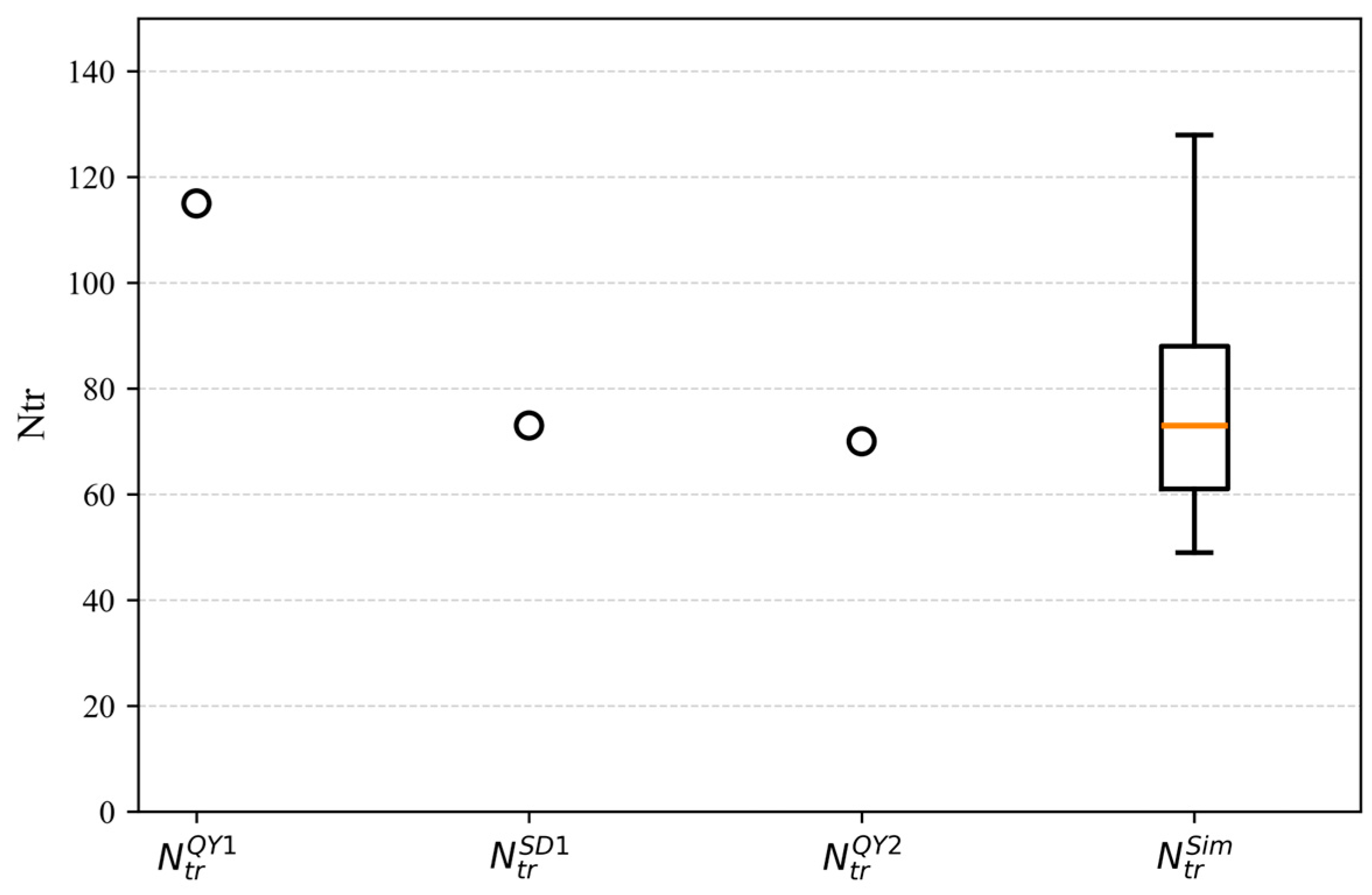
As shown in Figure 10, the distribution of $N_{\mathrm{t}\mathrm{r}}^{\mathrm{S}\mathrm{i}\mathrm{m}}$ computed from all vertical grid columns in the analyzed realization has a median of approximately 70, an interquartile range of about 60–90, and a spread of roughly 50–130. The well-based transition counts $N_{\mathrm{t}\mathrm{r}}^{\mathrm{W}\mathrm{e}\mathrm{l}\mathrm{l}}$ for SD1, QY2, and QY1 fall within this modeled distribution; SD1 and QY2 are close to the median, whereas QY1 is located in the upper part of the range but remains within the simulated variability. 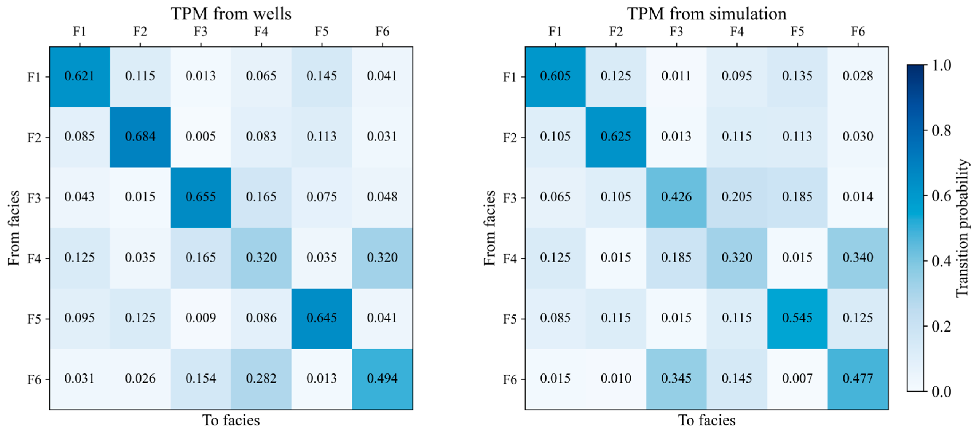Complementarily, the TPM comparison (Figure 11) evaluates the facies-to-facies switching tendencies in the same realization using a first-order Markov framework, yielding $D_{\mathrm{M}\mathrm{A}\mathrm{E}}=0.0396$ relative to the well-derived TPM. Taken together, the transition-count and TPM statistics indicate that the realization preserves the intensity of bedding-scale facies alternations without an artificially smoothed vertical rhythm.

3.3.3. Global Facies Proportions

To examine whether the 3D model yields a reasonable facies composition at the global scale, we generate 10 independent realizations and compute the volumetric fraction of each facies in every realization. For the $r$-th realization, the global proportion of facies $k$, $f_k^{\left(r\right)}$, is defined in Equation (6) as the ratio between the number of cells assigned to facies $k$ and the total number of cells in the counting domain:

$$f_k^{\left(r\right)}={\displaystyle \frac{N_k^{\left(r\right)}}{N}},k=1,\dots ,6,r=1,\dots ,10$$

(6)

Here, $N_k^{\left(r\right)}$ denotes the number of grid cells classified as the $k$-th facies in realization $r$, and $N$ is the total number of grid cells in the domain. The global facies proportions are then summarized across realizations by their ensemble mean, ${\bar{f}}_k$, computed according to Equation (7):

$${\bar{f}}_k={\displaystyle \frac{1}{10}}\sum _{r=1}^{10}{f}_k^{\left(r\right)},k=1,\dots ,6$$

(7)

The well-based proportion $f_k^{\mathrm{well}}$ is computed by merging the facies sequences from the three wells at the same vertical discretization and counting the corresponding facies frequencies. By comparing ${\bar{f}}_k$ with $f_k^{\mathrm{well}}$, we evaluate whether the simulations preserve a facies composition that is globally consistent with the well interpretations, and whether any facies has been systematically overrepresented or underrepresented during simulation.

As shown in

Table 5. Comparison of facies volumetric fractions between the 3D model and well data (${\bar{f}}_k$ vs. $f_k^{\mathrm{w}\mathrm{e}\mathrm{l}\mathrm{l}}$).

Facies	Model Volumetric Fraction (${\bar{\mathit{f}}}_{\mathit{k}}$)	Well-Based Proportion (${\mathit{f}}_{\mathit{k}}^{\mathbf{w}\mathbf{e}\mathbf{l}\mathbf{l}}$)	Difference ($\mathsf{\Delta }{\mathit{f}}_{\mathit{k}}={\bar{\mathit{f}}}_{\mathit{k}}-{\mathit{f}}_{\mathit{k}}^{\mathbf{well}}$)
1	0.3245	0.3479	−0.0234
2	0.3934	0.3698	+0.0236
3	0.0187	0.0295	−0.0108
4	0.0461	0.0418	+0.0043
5	0.1864	0.1791	+0.0073
6	0.0309	0.0317	−0.0008

, the volumetric-fraction comparison based on the mean proportions of 10 realizations indicates that the simulated global facies composition is broadly consistent with the well-derived proportions. The absolute differences $\mid \mathsf{\Delta }{f}_k\mid$ range from 0.0008 to 0.0236, with the maximum deviation observed for Facies 2. Such small discrepancies are expected to some extent due to an upscaling effect, because $f_k^{well}$ is estimated from three 1D well trajectories whereas ${\bar{f}}_k$ represents a 3D volumetric statistic over the entire grid. Overall, the results indicate that the workflow does not introduce a pronounced global bias in facies proportions, supporting the use of the realizations for subsequent structural interpretation and uncertainty analysis.

3.3.4. Connectivity Metrics

Connectivity is a key structural attribute for shale-reservoir interpretation because it indicates whether lithofacies bodies form laterally continuous units or occur as isolated patches, which is relevant for subsequent flow-related and geomechanical assessments [33]. To address this requirement, we quantify connected geobodies for the three volumetrically dominant lithofacies in the analyzed realization—Organic-lean laminated mudstone (Facies 1), Organic-lean bedded mudstone (Facies 2), and Organic-rich bedded mudstone (Facies 5)—on a simulation grid of $73\times 31\times 1351$ cells.

Connected geobodies are identified using 6-neighborhood (face) connectivity, which provides a conservative definition by considering only face-adjacent cells as connected. For each facies $k$, cells belonging to $k$ are grouped into connected components, and connectivity is summarized by the number of geobodies ($N_g$) and the largest connected fraction (LCF), defined as the ratio of the largest geobody volume to the total volume of the target facies. In addition, percolation is evaluated along the $x$, $y$, and $z$ directions and reported as True if at least one geobody connects the two opposite model boundaries in that direction.

As summarized in

Table 6. Connectivity metrics of connected geobodies for the dominant lithofacies (6-neighborhood). Connected geobodies are identified using 6-neighborhood connectivity. LCF denotes the largest connected fraction, defined as the voxel count of the largest geobody divided by the total voxel count of the corresponding facies. Percolation indicates boundary-to-boundary connectivity, i.e., whether at least one geobody spans the model domain between opposite.

Facies	Total Voxels (N)	Num of Geobodies (Ng)	Largest Geobody (Voxels)	LCF	Percolation (x/y/z)
1	987,181	8021	713,374	0.7226	True/True/False
2	1,345,425	3926	870,538	0.6470	True/True/False
5	715,475	15,037	288,879	0.4038	True/True/False

, Facies 1 (organic-lean laminated mudstone) and Facies 2 (organic-lean bedded mudstone) exhibit strong connectivity, with LCF values of 0.7226 and 0.6470, respectively. Both facies percolate laterally in the $x$ and $y$ directions but do not percolate vertically ($z=$ False), consistent with shale architectures where laminated and bedded units tend to extend along stratification while frequent vertical alternations interrupt vertical continuity. In contrast, Facies 5 (organic-rich bedded mudstone) shows a lower LCF (0.4038), indicating comparatively more segmented connectivity, although it still percolates laterally ($x$ and $y=$True). Meanwhile, the large numbers of connected geobodies ($N_g$) identified for these dominant facies (Table 6) indicate that, in addition to a laterally continuous connected framework, numerous small isolated patches are present, reflecting frequent bedding-scale lithofacies alternations and partitioning. This pattern is consistent with the thin interbedding and high-frequency vertical variability that typify shale successions in the F2 interval.

4. Discussion

The proposed workflow targets a practical difficulty frequently encountered in shale-reservoir modeling: high-frequency vertical facies alternations and stratified architectures must be reproduced under sparse well control, while representative 3D training images are typically unavailable. The quantitative evaluation in Section 3.3 provides insight into what aspects of shale heterogeneity are effectively captured by the workflow and why these metrics are meaningful beyond visual plausibility.

A key feature of the F2 shale interval is the frequent bedding-scale alternation of lithofacies, which manifests as rapid vertical switching and thin interbedding. In such settings, a 3D facies model can appear laterally coherent while still being unrealistic if the vertical rhythm is overly smoothed. The vertical transition count $N_{\mathrm{t}\mathrm{r}}$ therefore serves as a direct indicator of whether the realization maintains the intensity of bedding-scale variability observed in the wells. The fact that the well-based transition counts fall within the distribution of $N_{\mathrm{t}\mathrm{r}}^{\mathrm{S}\mathrm{i}\mathrm{m}}$ computed from the realization indicates that the workflow does not suppress vertical alternations during 2D-to-3D propagation. This matters because vertical alternations strongly control the effective thickness, continuity, and compartmentalization of facies packages, and consequently influence reservoir-scale interpretations derived from the model. In addition, transition counts alone do not reveal which facies-to-facies switches dominate; the transition probability matrix (TPM) complements $N_{\mathrm{t}\mathrm{r}}$ by quantifying the directional switching tendencies between facies classes. The relatively small TPM discrepancy ($D_{\mathrm{M}\mathrm{A}\mathrm{E}}=0.0396$) suggests that the realization reproduces not only the frequency of transitions but also the dominant alternation patterns inferred from the well sequences, providing a more stringent, statistics-based check on thin-interbedding reproduction.

The reliance on vertical 2D sections as TI carriers in this study should be understood as a feasibility-driven strategy rather than an assertion that 2D sections are universally superior to 3D TIs. In the present field setting, high-quality 3D TIs are not available, and constructing them artificially is particularly challenging for shale systems. Unlike fluvial or channelized reservoirs where object-based or process-based rules can generate plausible 3D architectures with relatively limited degrees of freedom, shale facies architectures are often governed by subtle bedding-scale stacking, frequent vertical alternations, and laterally extensive but internally heterogeneous stratification. These characteristics are difficult to encode reliably into a synthetic 3D TI without introducing subjective geometric assumptions or over-idealized structures. By contrast, well-constrained vertical sections can directly preserve the observed vertical rhythm and lithofacies stacking characteristics, and s2Dcd provides a mechanism to propagate these section-based patterns into 3D space while still honoring hard well constraints. In this sense, the workflow aims to reduce the dependence on subjective 3D TI design by leveraging the most reliable information available in data-limited shale settings: well-controlled vertical stacking patterns and section-scale stratified structures.

The connected-geobody results further support the stratified nature of the realizations. For the dominant lithofacies, lateral percolation in the $x$ and $y$ directions combined with the absence of vertical percolation is consistent with shale architectures where facies bodies extend preferentially along stratification and are vertically interrupted by frequent alternations. At the same time, the coexistence of a dominant connected component (as quantified by LCF) with a large number of smaller components reflects the expected partitioning induced by thin interbeds and stacking variability, complementing the TPM-based assessment from a geometric connectivity perspective.

In comparison with alternative facies-modeling options, a rigorous method-to-method benchmark is constrained by the available data. Conventional 3D MPS cannot be tested because it requires a representative 3D training image, which is unavailable for the study block and difficult to construct for shale successions without introducing subjective geometric assumptions. Under these constraints, the most meaningful baseline is a two-point variogram-based indicator approach derived from well statistics; however, two-point methods mainly reproduce covariance structure and therefore tend to yield overly smooth transitions, making it difficult to preserve the thinly layered, rhythmically alternating shale architectures observed in the wells [34,35]. Accordingly, our workflow provides a data-feasible yet high-fidelity solution for shale settings by consistently reproducing well-observed vertical rhythmicity and stratified architectures under strict hard conditioning, while maintaining realistic interbedding characteristics beyond what two-point baselines typically capture.

Several limitations should be noted. First, only three wells are available in the study area, and all of them are required to construct the orthogonal vertical sections that serve as TI carriers; therefore, an independent blind-well validation is not feasible in the present dataset. Second, rare facies classes may yield less stable transition statistics because of limited samples in the well data, which can affect individual TPM entries. Third, the workflow is designed for settings where vertical section information is meaningful; if the target reservoir exhibits strongly non-stratified 3D architectures, additional constraints (e.g., dense seismic-derived structures) may be required. Despite these limitations, the proposed workflow provides a reproducible and data-feasible solution for 3D shale facies modeling in the absence of representative 3D TIs, while explicitly quantifying the reproduction of bedding-scale alternations and stratified connectivity.

5. Conclusions

This study addresses the 3D shale facies modeling challenge posed by sparse well control and the lack of representative 3D training images (TIs) for the F2 Member in the Qintong Sag. A reproducible hierarchical workflow was developed, consisting of (i) constructing well-constrained vertical 2D facies sections as TI carriers using MIXSIM and (ii) propagating the sectional patterns into 3D space using an s2Dcd strategy with hard well conditioning. The workflow is designed to preserve a key shale characteristic—frequent bedding-scale facies alternations—while enabling practical 3D modeling when 3D TIs are unavailable or difficult to construct for stratified shale architectures.

The case study demonstrates that the proposed workflow generates 3D facies realizations that exactly honor conditioning data at well locations and reproduce shale-like vertical transition behavior in a statistically explicit manner. In particular, the first-order transition probability matrix derived from a representative realization shows close agreement with the well-derived TPM, with a mean absolute error of $D_{\mathrm{M}\mathrm{A}\mathrm{E}}=0.0396$, indicating that dominant facies-switching tendencies associated with thin interbedding are preserved beyond transition-count similarity alone. At the global scale, facies volumetric fractions averaged over 10 realizations remain close to the well-based proportions, with a maximum deviation of 2.36%, suggesting that no pronounced bias in overall facies composition was introduced during simulation. Connectivity analysis based on connected geobodies further indicates laterally extensive stratified architectures for the dominant facies, characterized by lateral percolation in the $x-y$ directions and interrupted vertical continuity, consistent with shale depositional layering.

From a reservoir-management perspective, this hierarchical “vertical-section-driven 2D-to-3D” strategy provides a practical route to build geologically interpretable 3D facies frameworks for data-limited shale intervals. By preserving bedding-scale alternations, global composition, and lateral connectivity trends, the resulting models offer an improved structural basis for subsequent tasks such as identifying laterally persistent target intervals, defining stratigraphic compartments, and evaluating scenario-based uncertainty using multiple realizations. The accuracy of the facies framework directly impacts these outcomes: biases in stratigraphic continuity and facies proportions can misidentify laterally persistent targets and compartments, while misrepresented connectivity and intra-layer heterogeneity propagate into downstream property modeling and engineering predictions by altering inferred pathways and uncertainty ranges. Future work should incorporate additional wells and seismic-derived constraints to strengthen interwell control and integrate soft conditioning information to further support engineering-oriented predictions.

References

- Jin, Z.; Wang, G.; Liu, G.; Gao, B.; Liu, Q.; Wang, H.; Liang, X.; Wang, R. Research Progress and Key Scientific Issues of Continental Shale Oil in China. Acta Pet. Sin. 2021, 42, 821–835. [Google Scholar] [CrossRef]
- Bai, B.; Dai, C.; Hou, X.; Yang, L.; Wang, R.; Wang, L.; Meng, S.; Dong, R.; Liu, Y. Geological Heterogeneity of Shale Sequence and Evaluation of Shale Oil Sweet Spots in the Qingshankou Formation, Songliao Basin. Oil Gas Geol. 2023, 44, 846–856. [Google Scholar] [CrossRef]
- Jiang, Z.; Zhang, J.; Kong, X.; Xie, H.; Cheng, H.; Wang, L. Research Progress and Development Direction of Continental Shale Oil and Gas Deposition and Reservoirs in China. Acta Pet. Sin. 2023, 44, 45–71. [Google Scholar] [CrossRef]
- Fang, Z.; Pu, X.; Chen, S.; Yan, J.; Yang, H.; Ma, B.; Dong, Q. Impact of Multi-Scale Laminae Characteristics on Lacustrine Shale Reservoir Quality: A Case Study from the Second Member of the Kongdian Formation in the Cangdong Sag, Bohai Bay Basin, China. Geol. J. 2025, 1, 1–22. [Google Scholar] [CrossRef] [Scilit]
- Liu, X.; Liu, J.; Wang, X.; Guo, Q.; Lv, Q.; Yang, Z.; Zhang, Y.; Zhang, Z.; Zhang, W.; Zhang, W. Mechanisms of Fine-Grained Sedimentation and Reservoir Characteristics of Shale Oil in a Continental Freshwater Lacustrine Basin: A Case Study from the Chang 73 Sub-Member of the Triassic Yanchang Formation in Southwestern Ordos Basin, NW China. Pet. Explor. Dev. 2025, 52, 95–111. [Google Scholar] [CrossRef] [Scilit]
- Zhao, L.; Hu, C.; Quaye, J.A.A.; Lu, N.; Peng, R.; Zhu, L. Comparative Analysis of 3D Reservoir Geologic Modeling: A Comprehensive Review and Perspectives. Geoenergy Sci. Eng. 2025, 244, 213440. [Google Scholar] [CrossRef] [Scilit]
- Shu, Z. Shale Reservoir 3D Structural Modeling Using Horizontal Well Data: Main Issues and an Improved Method. Front. Earth Sci. 2021, 9, 695502. [Google Scholar] [CrossRef] [Scilit]
- Liu, H. Characteristics of Lithofacies Combinations and Reservoir Property of Carbonate-Rich Shale in Dongying Depression, Eastern China. Front. Earth Sci. 2022, 10, 857729. [Google Scholar] [CrossRef] [Scilit]
- Dong, S.; Yang, X.; Xu, T.; Zeng, L.; Qu, K.; Chen, Q.; Wang, L.; Zhang, F.; Bai, X. Generative Adversarial Networks for Improved Three-Dimensional Reservoir Modeling: Image Processing-Inspired Approaches and Their Effects on Different Well Data Levels. Math. Geosci. 2026. [Google Scholar] [CrossRef] [Scilit]
- Staněk, F.; Franěk, J.; Jelínek, J.; Žáček, V. Estimating Relative Uncertainty of Geological 3D Models with Low Density of Input Data in Geologically Complex Regions. Earth Sci. Inform. 2025, 18, 259. [Google Scholar] [CrossRef] [Scilit]
- Li, N.; Feng, Z.; Wu, H.; Tian, H.; Liu, P.; Liu, Y.; Liu, Z.; Wang, K.; Xu, B. New Advances in Methods and Technologies for Well Logging Evaluation of Continental Shale Oil in China. Acta Pet. Sin. 2023, 44, 28–44. [Google Scholar] [CrossRef]
- Zhao, D. Considerations on Application Strategies of Geophysical Techniques for Lacustrine Shale Oil Exploration and Development. Geophys. Prospect. Pet. 2022, 61, 963–974. [Google Scholar] [CrossRef]
- Liu, X.; Wang, X.; Liu, Y.; Zhang, J.; Liu, J.; Liu, Q. Current Status and Development Direction of Seismic Prospecting Technology for Continental Shale Oil in China. Acta Pet. Sin. 2023, 44, 2270–2285. [Google Scholar] [CrossRef]
- Guardiano, F.B.; Srivastava, R.M. Multivariate Geostatistics: Beyond Bivariate Moments. In Geostatistics Troia ’92; Soares, A., Ed.; Springer: Dordrecht, The Netherlands, 1993; pp. 133–144. [Google Scholar] [CrossRef] [Scilit]
- Strebelle, S. Conditional Simulation of Complex Geological Structures Using Multiple-Point Statistics. Math. Geol. 2002, 34, 1–21. [Google Scholar] [CrossRef] [Scilit]
- Mariethoz, G.; Renard, P.; Straubhaar, J. The Direct Sampling Method to Perform Multiple-Point Geostatistical Simulations. Water Resour. Res. 2010, 46, W11536. [Google Scholar] [CrossRef] [Scilit]
- Mariethoz, G.; Caers, J. Multiple-Point Geostatistics: Stochastic Modeling with Training Images; Wiley: Hoboken, NJ, USA, 2014. [Google Scholar] [CrossRef] [Scilit]
- Bhavsar, F.; Desassis, N.; Ors, F.; Romary, T. A Stable Deep Adversarial Learning Approach for Geological Facies Generation. Comput. Geosci. 2024, 190, 105638. [Google Scholar] [CrossRef] [Scilit]
- Yao, J.; Liu, Y.; Pan, M. Research on the Construction Method of a Training Image Library Based on cDCGAN. Appl. Sci. 2023, 13, 9807. [Google Scholar] [CrossRef] [Scilit]
- Maharaja, A. TiGenerator: Object-Based Training Image Generator. Comput. Geosci. 2008, 34, 1753–1761. [Google Scholar] [CrossRef] [Scilit]
- Chen, Q.; Mariethoz, G.; Liu, G.; Comunian, A.; Ma, X. Locality-Based 3-D Multiple-Point Statistics Reconstruction Using 2-D Geological Cross Sections. Hydrol. Earth Syst. Sci. 2018, 22, 6547–6566. [Google Scholar] [CrossRef] [Scilit]
- Deutsch, C.V.; Tran, T.T. FLUVSIM: A Program for Object-Based Stochastic Modeling of Fluvial Depositional Systems. Comput. Geosci. 2002, 28, 525–535. [Google Scholar] [CrossRef] [Scilit]
- Comunian, A.; Renard, P.; Straubhaar, J. 3D Multiple-Point Statistics Simulation Using 2D Training Images. Comput. Geosci. 2012, 40, 49–65. [Google Scholar] [CrossRef] [Scilit]
- Hou, W.; Liu, H.; Zheng, T.; Chang, H.; Xiao, F. Extended GOSIM: MPS-Driven Simulation of 3D Geological Structure Using 2D Cross-Sections. Earth Space Sci. 2022, 9, e2021EA001801. [Google Scholar] [CrossRef] [Scilit]
- Cordua, K.S.; Hansen, T.M.; Gulbrandsen, M.L.; Mosegaard, K. Mixed-Point Geostatistical Simulation: A Combination of Two- and Multiple-Point Geostatistics. Geophys. Res. Lett. 2016, 43, 9030–9037. [Google Scholar] [CrossRef] [Scilit]
- Gao, Y.; Cai, X.; Xia, W.; Wu, Y.; Chen, Y. Characteristics of Reservoir Space and Sweet Spot Evaluation of Shale Oil in the Second Member of Paleogene Funing Formation in Subei Basin: A Case Study of Well QY1 in Qintong Sag. Pet. Geol. Exp. 2024, 46, 916–926. [Google Scholar] [CrossRef]
- Zan, L.; Luo, W.; Yin, Y.; Jing, X. Formation Conditions of Shale Oil and Favorable Targets in the Second Member of Paleogene Funing Formation in Qintong Sag, Subei Basin. Pet. Geol. Exp. 2021, 43, 233–241. [Google Scholar] [CrossRef]
- Xia, X.; Ma, X.; Hu, W.; Zang, S. Petrological Characteristics, Reservoir Property and Oil-Bearing Potential of Intrusive Rocks in Well Shaduo 1, Qintong Sag, Subei Basin. Pet. Geol. Exp. 2024, 46, 87–97. [Google Scholar] [CrossRef]
- Levy, S.; Friedli, L.; Mariéthoz, G.; Linde, N. Conditioning of Multiple-Point Statistics Simulations to Indirect Geophysical Data. Comput. Geosci. 2024, 187, 105581. [Google Scholar] [CrossRef] [Scilit]
- Manzocchi, T.; Walsh, D.A. Vertical Stacking Statistics of Multi-Facies Object-Based Models. Math. Geosci. 2023, 55, 461–496. [Google Scholar] [CrossRef] [Scilit] [PubMed]
- Hu, L.Y.; Chugunova, T. Multiple-Point Geostatistics for Modeling Subsurface Heterogeneity: A Comprehensive Review. Water Resour. Res. 2008, 44, W11413. [Google Scholar] [CrossRef] [Scilit]
- Feng, R.; Luthi, S.M.; Gisolf, D. Simulating Reservoir Lithologies by an Actively Conditioned Markov Chain Model. J. Geophys. Eng. 2018, 15, 800–815. [Google Scholar] [CrossRef] [Scilit]
- Pirot, G.; Joshi, R.; Giraud, J.; Lindsay, M.D.; Jessell, M.W. loopUI-0.1: Indicators to Support Needs and Practices in 3D Geological Modelling Uncertainty Quantification. Geosci. Model Dev. 2022, 15, 4689–4708. [Google Scholar] [CrossRef] [Scilit]
- Tahmasebi, P. Multiple Point Statistics: A Review. In Handbook of Mathematical Geosciences; Daya Sagar, B., Cheng, Q., Agterberg, F., Eds.; Springer: Cham, Switzerland, 2018; pp. 613–643. [Google Scholar] [CrossRef] [Scilit]
- Hashemi, S.; Javaherian, A.; Ataee-pour, M.; Khoshdel, H. Two-Point versus Multiple-Point Geostatistics: The Ability of Geostatistical Methods to Capture Complex Geobodies and Their Facies Associations—An Application to a Channelized Carbonate Reservoir, Southwest Iran. J. Geophys. Eng. 2014, 11, 065002. [Google Scholar] [CrossRef] [Scilit]
Figure 1.
Regional geological setting and structural location of the study area. Font colors indicate different geological features: uplift units are shown in purple, and structural or fault-related zones are shown in green.
Figure 2.
Regional structural framework and the distribution of the study area and wells. The gray shaded area indicates the modeling domain used in subsequent analyses. Font colors indicate different elements: place names and well are shown in black, and fault names are shown in red.
Figure 3.
3D modeling domain and well-data constraints in the study area (locations of wells QY1, QY2, and SD1 and their facies logs).
Figure 4.
Relationship among 1D well data, 2D sections, and 3D geological modeling. The figure illustrates the proposed workflow; the models shown are schematic and are not generated from real well data. Different colors represent different geological layers.
Figure 5.
Schematic illustration of the MIXSIM method (YZ section as an example). Circles denote conditioning nodes (hard data or previously simulated nodes). The vertical neighborhood provides a conditional distribution from multiple-point statistics, whereas the horizontal neighborhood provides a conditional distribution from two-point statistics. These two distributions are fused at the same location to obtain the final sampling probability.
Figure 6.
Schematic illustration of the s2Dcd method (using one XZ slice and one YZ slice as examples). Well data are first imposed in the 3D grid as hard conditioning information for subsequent simulation. Then, following a predefined slice path, conditional 2D simulations are performed sequentially on slices in the XZ and YZ directions, and the results of completed slices are propagated as conditioning information to the subsequent slices. By progressively traversing the XZ and YZ slice sequences and updating the conditioning data, a simulated realization that fills the entire 3D grid is ultimately obtained. The models shown are schematic and different colors represent different geological layers.
Figure 7.
Modeled vertical facies sections in the XZ and YZ directions constructed using the MIXSIM algorithm under hard conditioning to well data: (a) XZ section; (b) YZ section. Well columns are highlighted by black boxes and are preserved exactly during simulation because they are imposed as hard conditioning constraints.
Figure 8.
3D facies simulation results obtained using the s2Dcd method, with the XZ and YZ vertical sections as training images and well data imposed as hard conditioning.
Figure 9.
Representative slices in the XZ and YZ directions illustrating inter-slice continuity and 3D structural consistency across different orientations.
Figure 10.
Statistical distribution of the vertical transition counts in the 3D model and comparison with the well-based counts . The boxplot indicates a median (orange line) of approximately 70, an interquartile range of roughly 60–90, and an overall spread of about 50–130. The three wells fall within the modeled distribution; SD1 and QY2 are close to the median level, whereas QY1 shows a higher transition count but remains within the modeled range.
Figure 11.
Comparison of vertical transition probability matrices (TPMs) derived from (left) the merged facies sequences of the three wells and (right) a representative 3D realization. Each entry denotes the conditional probability of transitioning from facies to facies between adjacent vertical grid cells (first-order Markov chain). Matrix values are annotated in each cell, and the color intensity (light to dark blue) indicates increasing transition probability. The agreement between the two TPMs reflects how well the realization reproduces the directional facies-switching tendencies associated with thin interbedding in the F2 shale interval.