Article

An Engineering Framework for Adaptive Winglet Design: Identification of the Optimal Morphing Mode and Envelope


1
School of Air Transportation, Shanghai University of Engineering Science, Shanghai 201620, China
2
School of Civil, Aerospace and Design Engineering, Queen’s Building, University Walk, Bristol BS8 1TR, UK
3
School of Mechanical and Automotive Engineering, Shanghai University of Engineering Science, Shanghai 201620, China
*
Author to whom correspondence should be addressed.
Appl. Sci. 2026, 16(3), 1645; https://doi.org/10.3390/app16031645
Submission received: 27 December 2025 / Revised: 2 February 2026 / Accepted: 3 February 2026 / Published: 6 February 2026
(This article belongs to the Special Issue Morphing-Enabling Technologies for Aerospace Systems: 2nd Edition)

Featured Application

This work provides a practical framework for the preliminary design of adaptive winglets. The identified optimal morphing mode and corresponding morphing envelope provide direct guidance for the design of actuation mechanisms and control strategies for adaptive winglets.

Abstract

Adaptive winglets improve aerodynamic efficiency by enabling geometry adjustments tailored to flight conditions. In this study, an engineering-oriented optimization framework is developed and applied to numerical aerodynamic evaluations based on the wing–winglet configuration of a KC-135 aircraft, under representative takeoff, climb, and cruise conditions. A Plackett–Burman design is employed to screen the 10 kinds of winglet geometric parameters, from which the dominant variables affecting drag are identified. Subsequently, response surface methodology is used to construct surrogate models and determine optimal parameter combinations for each flight phase, thereby defining a feasible morphing envelope for adaptive winglet operation. The results indicate that a coupled morphing of winglet height and cant angle constitutes the most effective morphing mode. Across the takeoff, climb, and cruise phases, the optimal morphing envelope involves a continuous transition from Height = 0.20b/2 and Cant angle = 86.3° at takeoff, to Height = 0.192b/2 and Cant angle = 8.2° during climb, and finally approaching the baseline configuration (Height = 0.135b/2, Cant angle = 20°) at cruise, while achieving a maximum drag reduction efficiency improvement of up to 8.8% at the climb phase.

1. Introduction

Drag reduction is a key strategy in modern aviation for reducing fuel consumption, lowering operating costs, and minimizing pollutant emissions. Induced drag significantly impacts large aircraft, contributing approximately 40–50% of total drag during cruise and rising to 80–90% during takeoff and climb [1,2]. Therefore, reducing induced drag is critical for enhancing the performance of large aircraft. Although conventional fixed and blended winglets have been extensively studied and successfully applied to reduce induced drag, they are typically optimized for cruise conditions and are less effective during non-cruise phases such as takeoff and climb. This limitation is particularly notable for short-haul flights, where takeoff and climb constitute a significant portion of total flight time. In contrast, adaptive winglets can dynamically adjust their geometry, enabling optimal drag reduction across all flight phases [3,4,5,6].

1.1. Literature Review: Morphing Mode of the Adaptive Winglet

For adaptive winglets, the design problem differs fundamentally from that of conventional fixed or blended winglets. Instead of identifying a single optimal geometry, adaptive winglet design requires the selection of appropriate morphing modes and the definition of feasible morphing envelopes that can be implemented under different flight conditions.
From a geometric perspective, an adaptive winglet can be described by ten key parameters, including root chord, sweep angle, taper ratio, height, cant angle, toe angle, twist angle, area, aspect ratio, and airfoil, as illustrated in Figure 1. However, activating all parameters as morphing variables is neither practical nor necessary from an engineering standpoint. Determining which parameters should be selected as effective morphing variables to achieve meaningful drag reduction remains an open research question.
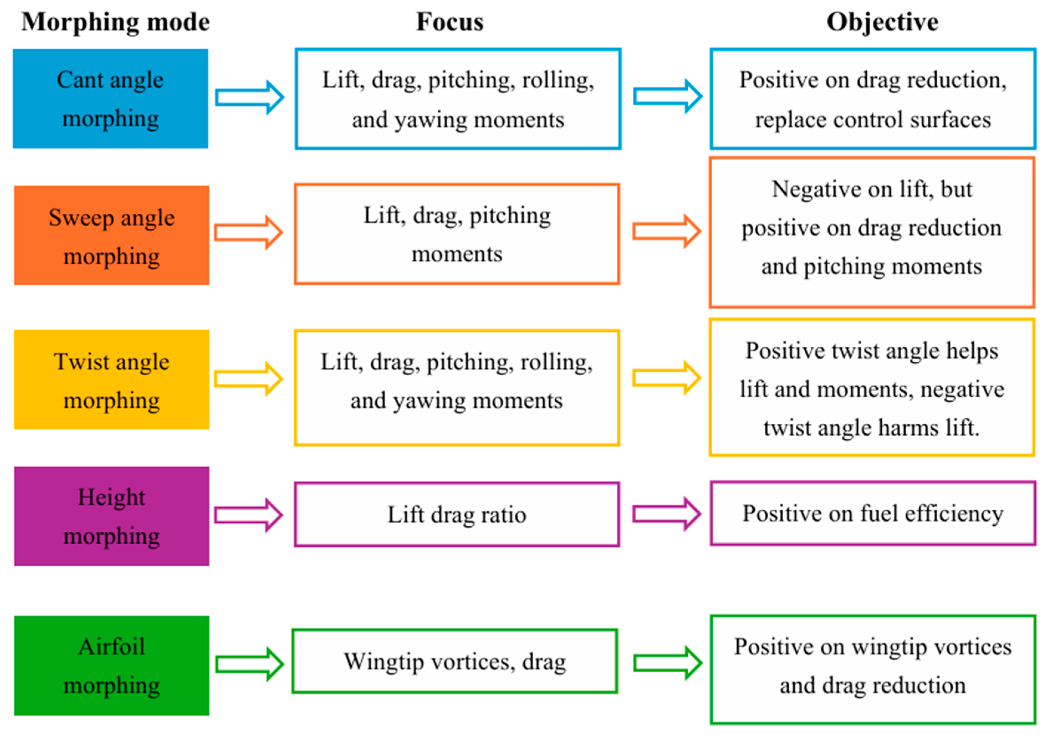
Based on published studies, existing research on adaptive winglets can be broadly categorized into five representative morphing modes, as summarized in Figure 2. These modes are reviewed below to highlight their aerodynamic characteristics and limitations, thereby motivating the need for a systematic comparison framework.
(a)
Cant angle morphing
Cant angle morphing has been implemented on the Boeing 777X; however, its application is currently restricted to ground operations for wingspan reduction and airport compatibility rather than in-flight aerodynamic optimization [7]. Nevertheless, several studies have explored the potential aerodynamic benefits of cant angle variation during flight. It has been reported that a moderate increase in cant angle during takeoff and climb can enhance lift, while further adjustment during cruise may improve drag reduction efficiency [8,9,10,11]. For example, a study on the CRJ700 aircraft with variable cant angle winglets demonstrated an improvement in lift-to-drag ratio of up to 6.10% and a reduction in drag coefficient of up to 2.65% [12]. In addition, morphing mechanisms enabling cant angle variation from −90° to 90° have been proposed [13], and applications on blended-wing-body UAVs have shown improvements in aerodynamic efficiency and stability [14].
Beyond aerodynamic performance, cant angle morphing has also been shown to generate pitching, rolling, and yawing moments, indicating its potential to supplement or partially replace conventional control surfaces [15,16]. A conceptual study was conducted on a morphing winglet with unsymmetrical stiffness, utilizing composite corrugation structures and finite element analysis to demonstrate that tailored stiffness distribution can optimize deformation under both aerodynamic and actuation loads [17]. However, existing studies typically focus on cant angle variation as an isolated morphing mode, without evaluating its relative effectiveness compared to other geometric parameters within a unified framework.
(b)
Sweep angle morphing
Sweep angle morphing has primarily been investigated as a means of improving aircraft control and aerodynamic performance, particularly for small-scale or unconventional aircraft configurations. Previous studies indicate that sweep variation can provide acceptable control authority and may serve as an alternative aircraft control methodology [18]. For large civil aircraft, sweep angle morphing has been reported to enhance aerodynamic performance during takeoff, cruise, and landing phases [19]. Nevertheless, the aerodynamic benefits of sweep angle morphing are often configuration-dependent, and its influence on induced drag reduction relative to other winglet parameters has not been systematically quantified.
(c)
Twist angle morphing
Twist angle morphing involves torsional deformation or geometric rotation along the winglet’s longitudinal axis, resulting in a relative change in airfoil orientation from root to tip. This morphing mode can alter the spanwise lift distribution and has been shown to enhance lift under certain conditions. However, the impact of twist angle morphing on drag reduction is more complex. While some studies report favorable aerodynamic effects, others indicate that excessive twist may lead to adverse drag penalties [20,21]. As a result, the effectiveness of twist angle morphing remains sensitive to both the magnitude of deformation and the operating condition, highlighting the need for quantitative optimization.
(d)
Height morphing
Height morphing directly modifies the effective wingspan and has been investigated on large transport aircraft such as the A380. Results indicate that height variation can lead to substantial reductions in fuel consumption, including approximately 3455 kg during cruise and 510 kg during climb, corresponding to a reduction of about 12,600 kg of CO2 emissions per flight [11,22]. Although height morphing is generally effective in reducing induced drag, increasing wingspan is subject to structural, weight, and airport compatibility constraints. Consequently, determining a feasible morphing envelope is critical for practical implementation.
(e)
Airfoil morphing
Airfoil morphing aims to modify the local aerodynamic characteristics and control wingtip vortex strength. Previous studies have shown that airfoil morphing can effectively reduce induced drag during climb and cruise, leading to fuel consumption and pollutant emission reductions of up to 6% [23,24,25]. Despite its demonstrated aerodynamic benefits, airfoil morphing often requires complex mechanisms and precise control, which may limit its applicability in large-scale transport aircraft. Furthermore, its effectiveness relative to other morphing modes has rarely been assessed within a comprehensive design framework.

1.2. Study Objectives

Despite the extensive investigations of individual morphing modes of adaptive winglets, two critical issues remain insufficiently addressed from an engineering design perspective. First, existing studies predominantly examine a single morphing parameter in isolation, making it difficult to identify which geometric variables should be selected as active morphing parameters when multiple candidates are available. Second, even when a morphing mode is identified, its feasible morphing envelope under different flight phases is rarely quantified systematically, limiting its practical applicability.
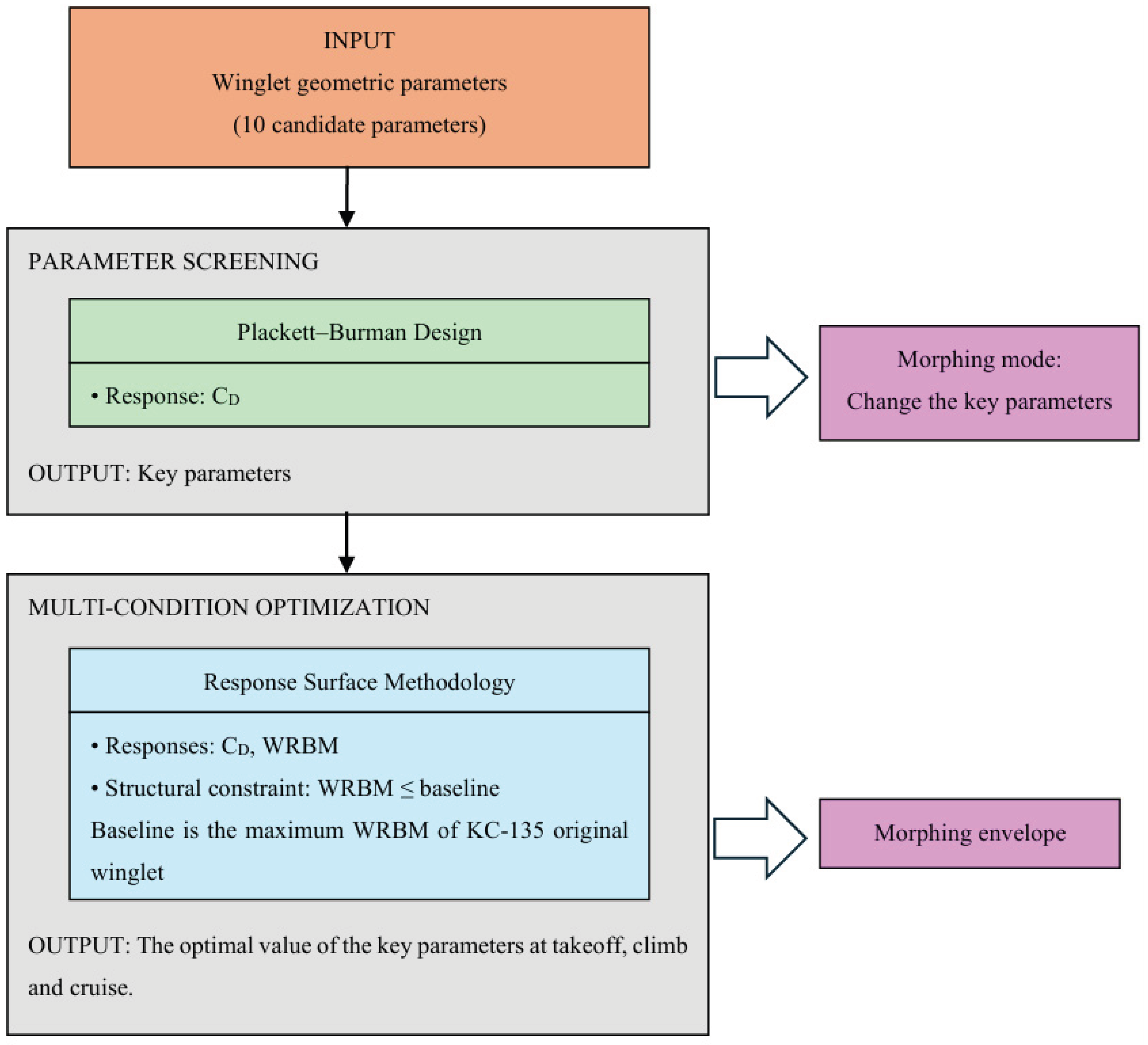
The objective of this study is to develop an engineering-oriented framework to address these issues by identifying both the optimal morphing mode and its corresponding morphing envelope for adaptive winglets. To achieve this objective, the study is conducted in three main steps. First, the Plackett–Burman design is employed to screen the geometric parameters of the winglet and identify the critical variables governing induced drag. Second, based on the selected parameters, response surface methodology is applied to determine the optimal parameter combinations for takeoff, climb, and cruise conditions. Finally, the results obtained for different flight phases are integrated to define a practical morphing envelope that can support adaptive winglet design and implementation. Figure 3 is the flowchart of this study. By providing a systematic comparison of morphing modes and a quantitative definition of feasible morphing envelopes, the proposed framework is intended to support preliminary aircraft design, morphing mode selection, and actuator constraint definition for adaptive winglets.

2. Materials and Methods

2.1. Wing and Winglet Configuration

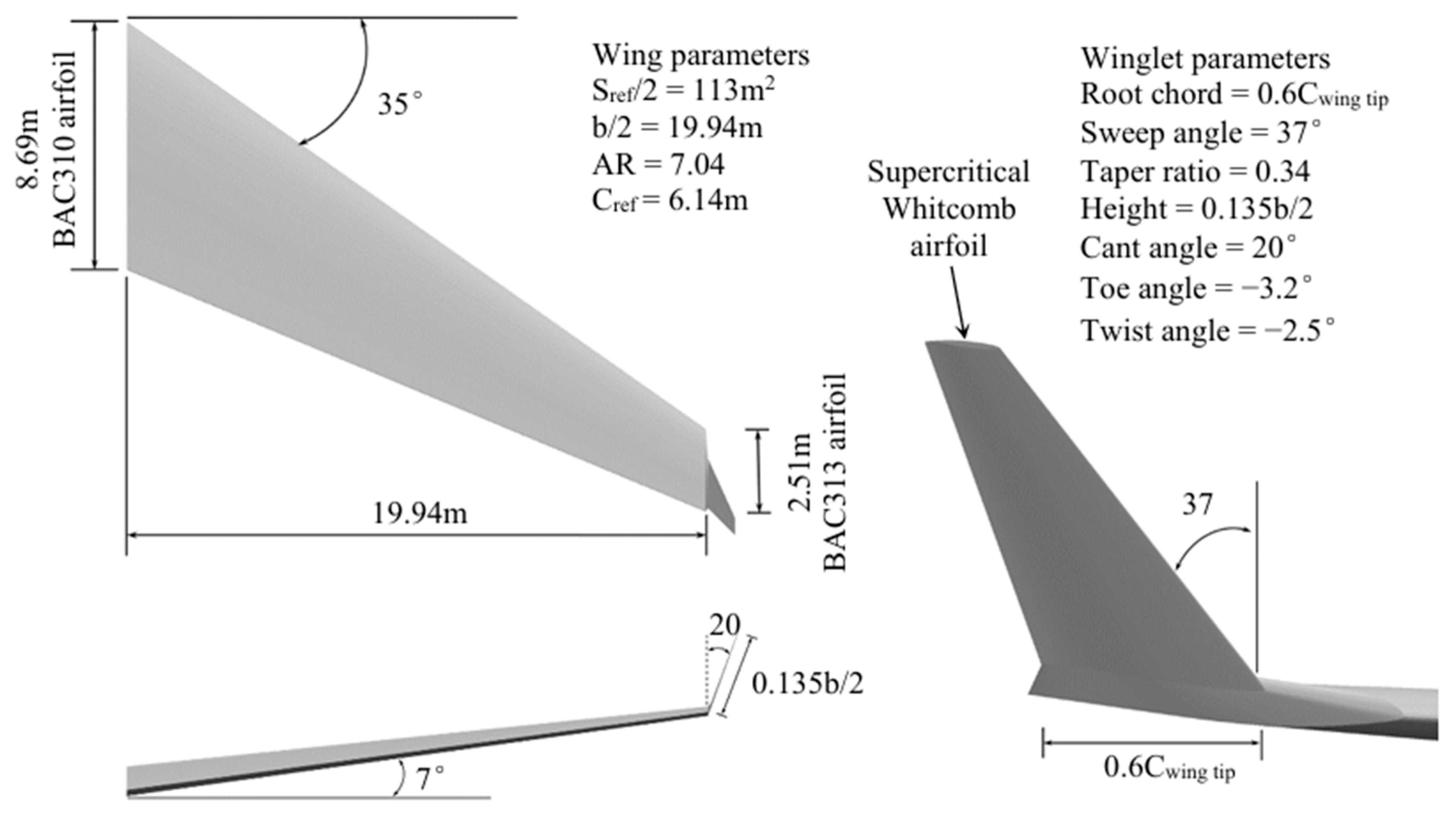
The KC-135 aircraft is selected as a benchmark configuration due to the availability of publicly documented geometric and aerodynamic data provided in Boeing technical reports [26]. These data enable independent verification of the aerodynamic modeling approach and provide a reliable reference for subsequent parametric studies. The KC-135 features a low-wing configuration equipped with an upward single-winglet design. The baseline winglet geometry is optimized for cruise conditions, corresponding to a free-stream Mach number of 0.78 and a lift coefficient of CL = 0.426. Under these conditions, the addition of winglets reduces the drag coefficient CD from 0.0240 to 0.0223, representing approximately a 7% drag reduction in cruise, as reported in Boeing documentation. The geometric parameters of the wing and winglet are illustrated in Figure 4.
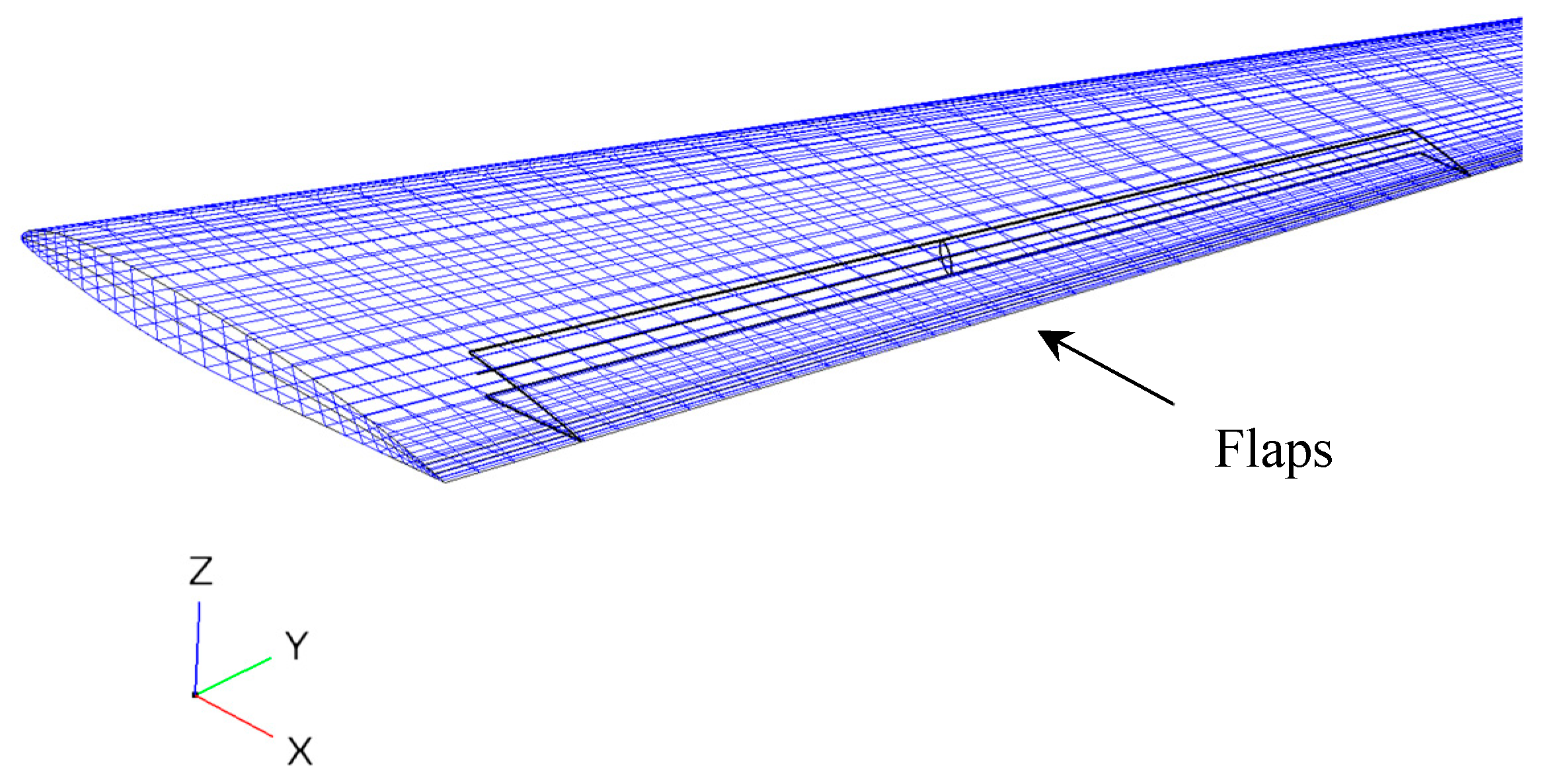
As the primary objective of this study is to evaluate the aerodynamic performance of adaptive winglets across different flight phases, the effects of high-lift devices are considered for low-speed conditions. In accordance with Boeing technical reports, trailing-edge flaps with deflection angles of 30° are applied for takeoff conditions, respectively, as shown in Figure 5. While the leading-edge slat is omitted from the analysis, its influence on winglet-induced drag trends is considered secondary relative to that of the trailing-edge flap and winglet geometry. This modeling approach enables a focused assessment of winglet morphing effects while ensuring consistency with the reference aerodynamic data.

2.2. Aerodynamic Modeling Approach

In this study, the aerodynamic performance of adaptive winglets is evaluated using a vortex lattice method (VLM) implemented in OpenVSP (version 3.40.1). In the vortex lattice method framework, lifting surfaces are represented by a distribution of horseshoe vortices, and the potential flow field is solved under the assumptions of inviscid, incompressible, and irrotational flow. Although viscous effects, flow separation, and shock-induced phenomena are not captured, the method offers high computational efficiency and reliably predicts lift distribution and induced drag trends. These characteristics make it well-suited for preliminary design and comparative analysis of winglet configurations.
To extend the applicability of the method to the transonic cruise conditions typical of the KC-135 aircraft, OpenVSP incorporates the Kármán–Tsien compressibility correction [27,28].
C P ( M a ,   α ,   c ,   f ) = C P ( 0 ,   α ,   c ,   f ) 1 M a 2 + M a 2 1 M a 2 + 1 C P ( 0 ,   α ,   c ,   f ) 2
where α represents the airfoil’s angle of attack, c represents the relative thickness of the airfoil, and f represents the relative camber of the airfoil.
This correction allows consistent aerodynamic evaluations across the takeoff, climb, and cruise phases while accounting for moderate compressibility effects. It should be noted that the present study does not aim to predict absolute drag values with high accuracy. Instead, the focus is on relative comparisons of drag reduction among different winglet morphing configurations, which is sufficient for identifying key design parameters, determining optimal morphing modes, and defining feasible morphing envelopes for adaptive winglets. The flow field boundary conditions are consistent with those in the Boeing report, as shown in Table 1.

2.3. Validation of the Aerodynamic Model

The validation strategy adopted in this study focuses on the ability of the aerodynamic model to predict relative drag variations induced by the installation of winglets, rather than absolute drag coefficients. This choice is motivated by the primary objective of the present work, which is to assess the aerodynamic benefits of adaptive winglet morphing through comparative analysis between different configurations. For such parametric studies, accurately capturing drag increments or reductions is more critical than achieving high-fidelity absolute drag predictions.
Accordingly, the validation is performed by comparing the predicted drag change between wing configurations with and without winglets under identical flight conditions. For the takeoff and cruise phases, OpenVSP results are compared with the corresponding drag increments reported in the Boeing KC-135 aerodynamic data [26], which provide a reliable reference for assessing the relative aerodynamic impact of winglet installation. For the climb phase, where no publicly available winglet drag increment data are reported, RANS CFD simulations are employed as an independent numerical reference. Prior to comparison, all aerodynamic models are calibrated to operate at the same prescribed lift coefficient by iteratively adjusting the angle of attack, ensuring that the evaluated drag differences are solely attributable to geometric effects rather than operating-point inconsistencies. Identical wing, winglet, and flap geometries, as well as consistent free-stream conditions, are maintained across OpenVSP and CFD simulations. The CFD Mesh and Solver Settings are listed in Appendix C.
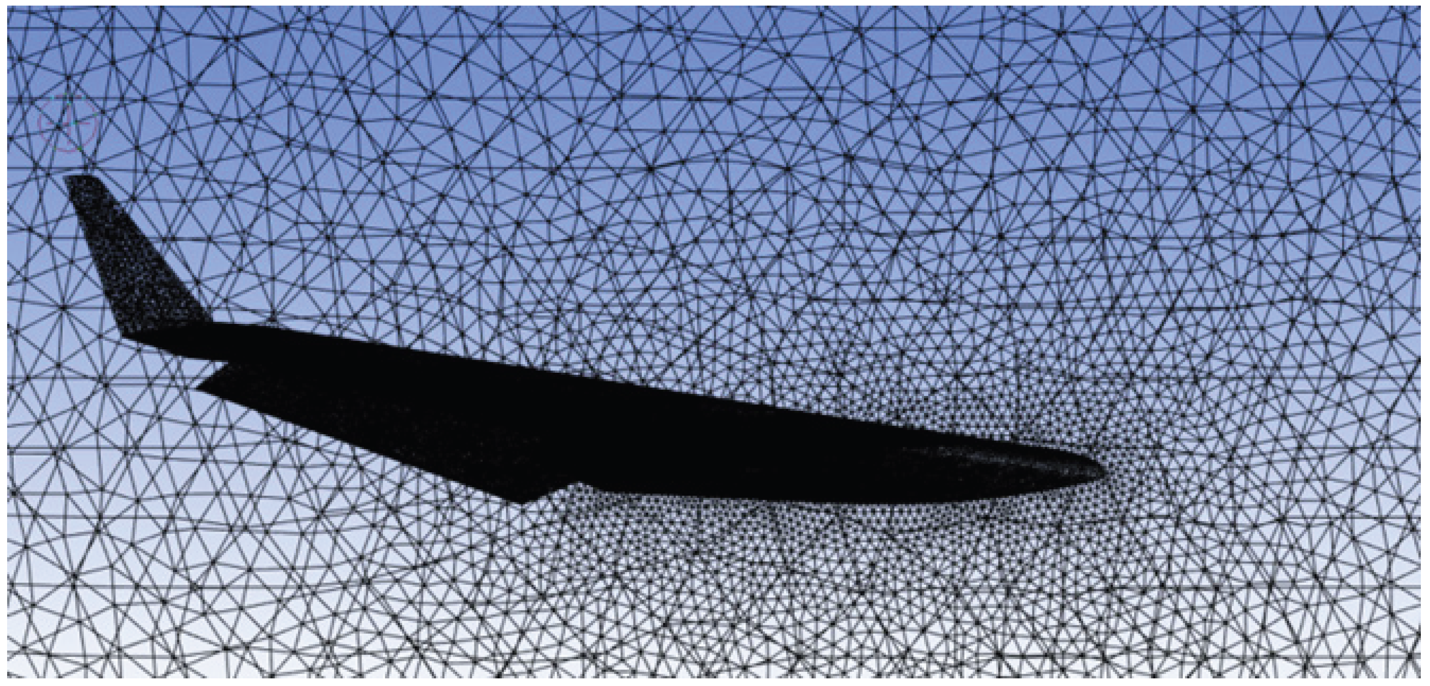
Figure 6 illustrates the CFD model, which includes the wing, winglet, and trailing-edge flap deflected downward by 30 degrees, configured consistently with the OpenVSP model. The CFD simulations are conducted at a free-stream Mach number of M = 0.40. Turbulence effects are modeled using the k–ω SST turbulence model, which is suitable for capturing global aerodynamic force trends for lifting surfaces under moderate-to-high lift conditions where localized flow separation may occur. A grid convergence study is performed to assess numerical robustness of the integrated aerodynamic coefficients. As summarized in Table 2, the variation in lift coefficient between the medium and fine meshes remains within 1.3%, indicating satisfactory grid convergence. Considering the marginal accuracy improvement obtained with further mesh refinement and the associated increase in computational cost, the medium-density mesh is therefore adopted for all subsequent CFD simulations, as it provides an appropriate balance between numerical accuracy and computational efficiency for the present validation study.
The validation results in Table 3 demonstrate that OpenVSP accurately captures the direction and magnitude of drag variation associated with winglet installation across the takeoff, climb, and cruise phases. Although discrepancies in absolute drag coefficients may exist due to differences in viscous modeling and geometric simplifications, the predicted relative drag changes remain consistent with the reference data, supporting the suitability of the OpenVSP-based aerodynamic model for comparative evaluation and parametric optimization of adaptive winglet configurations.

2.4. Identification of Key Parameters

Adaptive winglets involve multiple geometric parameters, many of which may influence induced drag in a coupled manner. However, simultaneous optimization of all parameters is neither computationally efficient nor physically necessary. Therefore, an initial parameter screening step is required to identify the key geometric variables that exert a dominant influence on drag reduction performance.
In this study, the Plackett–Burman design is employed as a screening tool to evaluate the relative importance of winglet geometric parameters. Plackett–Burman design is a two-level fractional factorial design method that enables efficient identification of significant main effects while neglecting higher-order interactions. This approach is well-suited for preliminary screening problems involving a large number of variables, where the objective is to reduce the dimensionality of the design space before detailed optimization. Based on the geometric definition of the winglet shown in Figure 1, ten parameters are initially considered, including root chord, sweep angle, taper ratio, height, cant angle, toe angle, twist angle, area, aspect ratio, and airfoil type. The high and low levels of each parameter are defined according to practical geometric constraints, existing winglet design practices, and ranges reported in the Boeing report, ensuring that all tested configurations remain physically feasible and aerodynamically meaningful.
The drag coefficient (CD) is selected as the primary response variable for the Plackett–Burman design, as induced drag reduction is the principal performance objective of adaptive winglets. For each Plackett–Burman design point, aerodynamic coefficients are computed using the validated aerodynamic model described in Section 2.2 and Section 2.3. The Plackett–Burman design assumes that main effects dominate the system response and that interaction effects are of secondary importance at this stage of analysis. Under this assumption, a linear regression model is constructed to quantify the influence of each geometric parameter on the drag coefficient [29], expressed as:
Y = β 0 + β i X i ( i = 1 ,   2 , ,   k )
where Y represents the response variable, Xi is the factors, β0 is the constant term of the regression equation, and βi is the regression coefficients.
The main effect level of the factor E(Xi) typically reflects Xi’s influence on Y.
E ( X i ) = 2 ( M i + M i ) N
where E(Xi) represents the main effect of Xi, Mi+, and Mi are the maximum and minimum values of Y observed in the experiment, respectively. N is the number of trials.
The significance of each parameter is evaluated based on the magnitude of its estimated main effect, which reflects the sensitivity of the drag coefficient to variations in that parameter. Parameters exhibiting negligible effects are excluded from further analysis, while those with dominant influence are retained as candidates for subsequent response surface optimization. Through this screening process, the dimensionality of the winglet morphing problem is substantially reduced, enabling a focused investigation of the most effective morphing modes and laying the foundation for the multi-condition optimization presented in the following section.

2.5. Optimization of Morphing Envelope

Following the identification of the dominant winglet parameters through the Plackett–Burman screening, response surface methodology is employed to determine the optimal morphing ranges of adaptive winglets under different flight conditions. Compared with direct multi-variable optimization methods, response surface methodology provides an efficient framework for modeling nonlinear relationships between design variables and aerodynamic responses while maintaining interpretability and computational efficiency. Based on the Plackett–Burman results, the winglet key parameters are selected as the independent design variables in the response surface analysis. The drag coefficient (CD) is selected as the primary response variable, while the wing root bending moment (WRBM) is introduced as a secondary response to ensure that aerodynamic improvements do not result in excessive structural loads.
Separate response surface methodology models are constructed for the takeoff, climb, and cruise flight conditions to account for the distinct aerodynamic characteristics associated with each phase. For each condition, a second-order polynomial regression model is fitted to describe the relationship between the design variables and the response variables [30], expressed as:
Y = β 0 + i = 1 k β i X i + i = 1 j 1 j = 1 k β i j X i X j + i = 1 k β i i X i 2
where Y represents the system response, β0, βi and βii are the intercept term, linear coefficient, and quadratic coefficient, respectively, βij is the interaction coefficient, Xi and Xj are the levels of the design variables.
Before modeling, all independent variables are transformed into dimensionless coded variables using linear normalization, mapping their physical ranges to the interval [ 1 ,   1 ] . This transformation ensures numerical stability of the regression process and allows for consistent comparison of variable sensitivities across different flight conditions. The statistical significance of the response surface models and regression coefficients is evaluated using analysis of variance (ANOVA). A response surface model is considered statistically acceptable when the overall model significance satisfies p 0.05 , while regression coefficients with p 0.25   are retained to preserve potentially influential terms, consistent with established response surface methodology practice in engineering optimization.
The optimal parameter combinations for each flight condition are obtained by minimizing the drag coefficient while maintaining the wing root bending moment within acceptable limits. By synthesizing the optimal solutions across takeoff, climb, and cruise conditions, a feasible morphing envelope is established, defining the allowable ranges of winglet height and cant angle that provide aerodynamic benefits throughout the entire flight profile. This response surface methodology-based optimization framework enables a quantitative definition of the optimal morphing mode and morphing envelope of adaptive winglets, providing practical design guidance for their implementation in real aircraft configurations.

3. Results

3.1. Definition of Winglet Parameter Space and Evaluation Metrics

This section defines the winglet parameter space adopted for the subsequent screening analysis and clarifies the aerodynamic evaluation metrics. Although a total of ten geometric parameters can be used to describe a winglet, as shown in Figure 1, not all of them are suitable as independent design variables in a screening study. The winglet airfoil is defined by discrete coordinate points and cannot be treated as a two-level factor within the Plackett–Burman design framework. In addition, the winglet area and aspect ratio are not independent parameters, as the combined effects of height, root chord, and taper ratio determine them. To avoid multicollinearity and ensure statistical independence among design factors, these parameters were excluded from the screening process. As a result, seven independent geometric parameters were retained for analysis: root chord, sweep angle, taper ratio, height, cant angle, toe angle, and twist angle. The parameter space was selected based on engineering feasibility and Boeing KC-135 aircraft winglet designs, ensuring that all configurations remain physically realizable. Following Boeing’s approach, the winglet height was normalized with respect to the half wingspan, as summarized in Table 4.
Using the Plackett–Burman design, the seven independent parameters were assigned numerical labels and evaluated at high and low levels. A total of twelve numerical experiments (N = 12) were conducted. The drag coefficient was adopted as the response variable and evaluated under a fixed lift coefficient condition of CL = 0.426, corresponding to the cruise lift requirement of the KC-135 aircraft. Under this controlled lift condition, the influence of individual geometric parameters on drag behavior could be isolated and assessed without interference from lift variations. For completeness and reproducibility, the detailed Plackett–Burman designs are provided in Appendix A.

3.2. Optimal Morphing Mode of Adaptive Winglets

3.2.1. Main Effects of Winglet Parameters on Drag Coefficient

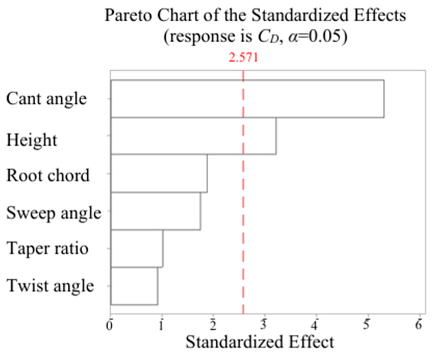
Figure 7 presents the Pareto chart of standardized effects from the Plackett–Burman design. Parameters with bars extending beyond the reference line (a = 0.05) are considered statistically significant. The response in the chart is the drag coefficient, and the design factors are the six parameters of the winglet. The cant angle and height of the winglet are key factors affecting the drag coefficient, while the other parameters are non-significant. Special note: The Pareto chart displays the significance of only six winglet parameters, whereas Section 3.1 explicitly states that seven parameters were included in the Plackett–Burman experiment. This discrepancy arises because the toe angle results in a p-value exceeding 0.05 in the regression model; the detailed explanation is provided in Appendix A.
The statistical significance levels of the winglet geometric parameters are summarized in Table 5. The results indicate that the cant angle and height exhibit a dominant influence on induced drag, while the remaining parameters show comparatively minor or negligible effects within the defined design space. This outcome confirms that drag reduction performance is governed primarily by a small number of key geometric features rather than by uniform contributions from all parameters. By reducing the original high-dimensional parameter space to a smaller set of influential variables, the Plackett–Burman analysis enables a focused investigation of adaptive winglet morphing mode without unnecessary design complexity.

3.2.2. Physical Interpretation of Key Parameters

According to the theoretical relationship given in Equation (8) [31], the induced drag coefficient is proportional to the square of the lift coefficient and inversely proportional to the wing aspect ratio. Among the seven independent winglet geometric parameters considered in this study, only increases in cant angle and winglet height can effectively enhance the wing’s effective aspect ratio, thereby achieving a reduction in the induced drag coefficient.
C D i = C L 2 π e A
where CDi is the induced drag coefficient, CL is the lift coefficient, A is the aspect ratio, and e is the Oswald efficiency factor accounting for deviations from the ideal elliptical lift distribution. For an ideal elliptical wing, e = 1, while for practical wings e < 1.
This aerodynamics-based physical interpretation not only corroborates the key parameters identified through the Plackett–Burman statistical screening, but also bridges the gap between statistical findings and practical winglet design. As a result, it provides a clear and robust theoretical justification for focusing subsequent optimization efforts on cant angle and height as the two key morphing variables.

3.2.3. Candidate Optimal Morphing Mode

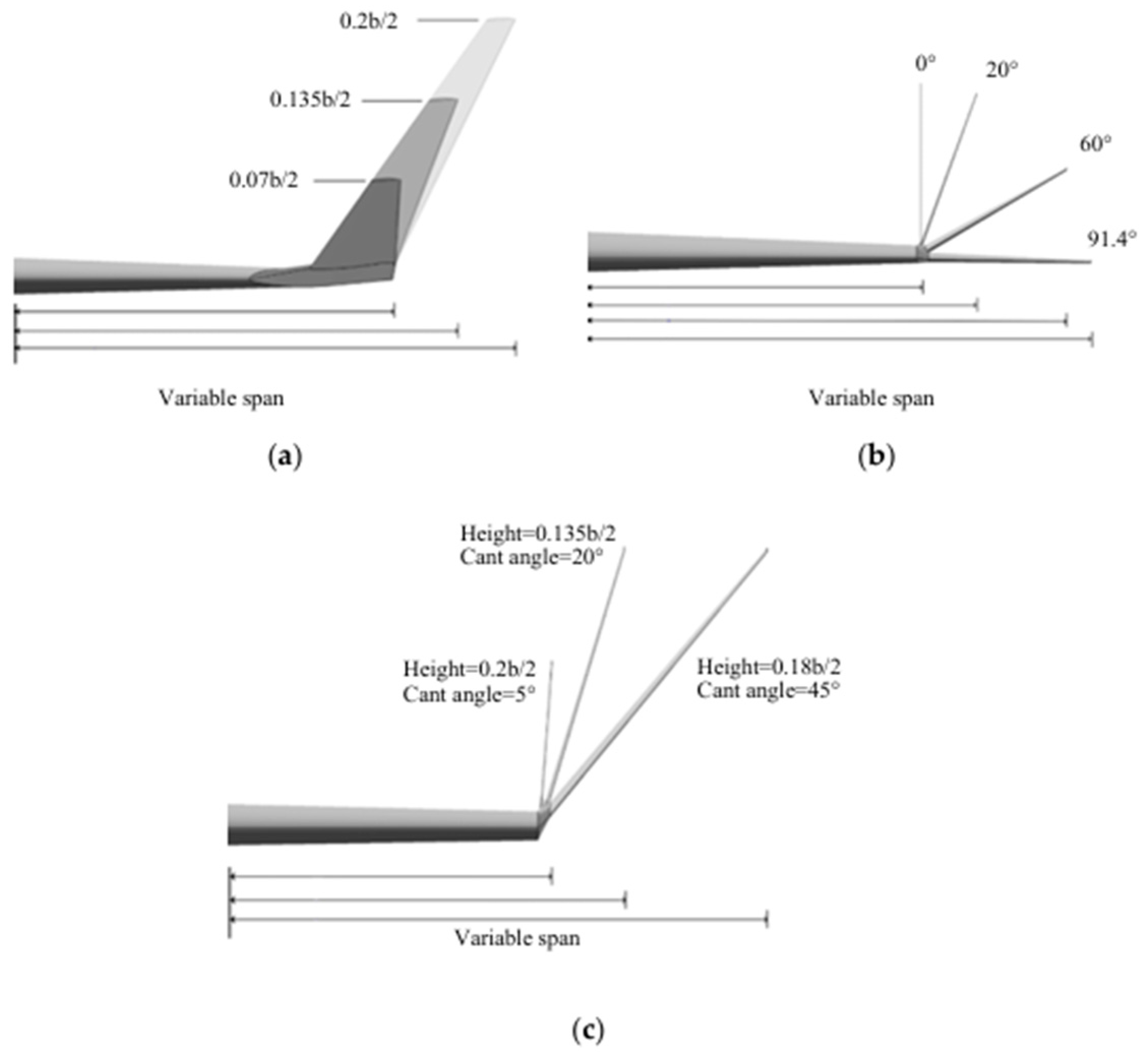
Adaptive winglets should adopt morphing strategies based on variations in cant angle and winglet height. Specifically, three morphing modes can be implemented: height-only morphing, cant-angle-only morphing, and combined morphing involving simultaneous adjustments of height and cant angle, as illustrated in Figure 8.
Under low-speed flight conditions where induced drag is dominant, increasing both the cant angle and winglet height enables the adaptive winglet to minimize induced drag while simultaneously generating additional lift. This enhanced lift capability allows the aircraft to climb more rapidly to cruise altitude with reduced thrust requirements, thereby improving fuel efficiency. In contrast, under high-speed flight conditions where parasitic drag becomes dominant, reducing the cant angle and winglet height decreases the effective frontal area of the wing, leading to a reduction in parasitic drag and improved aerodynamic efficiency during high-speed cruise.

3.3. Baseline Structural Constraint: Wing Root Bending Moment

While aerodynamic efficiency is the primary objective of adaptive winglet design, structural considerations impose essential constraints on feasible morphing modes. To account for structural loading effects, the wing root bending moment is evaluated as a secondary response variable. This study calculates the wing root bending moment by integrating the load at each spanwise station to obtain a specific value, according to Equation (6). At the same time, the effects of changes in winglet height and cant angle on the wing area and mean aerodynamic chord are also considered.
W R B M = 0 b / 2 ( 1 2 ρ v 2 × c l × C h o r d × Δ y × Y a v g )
where b/2 is the semi-span, v is the velocity, cl is the lift coefficient of a span station, Chord is the local chord of that station, Δy is the spanwise coordinate difference between that station and the adjacent station (the local span of that station), and Yavg is the span of that station.
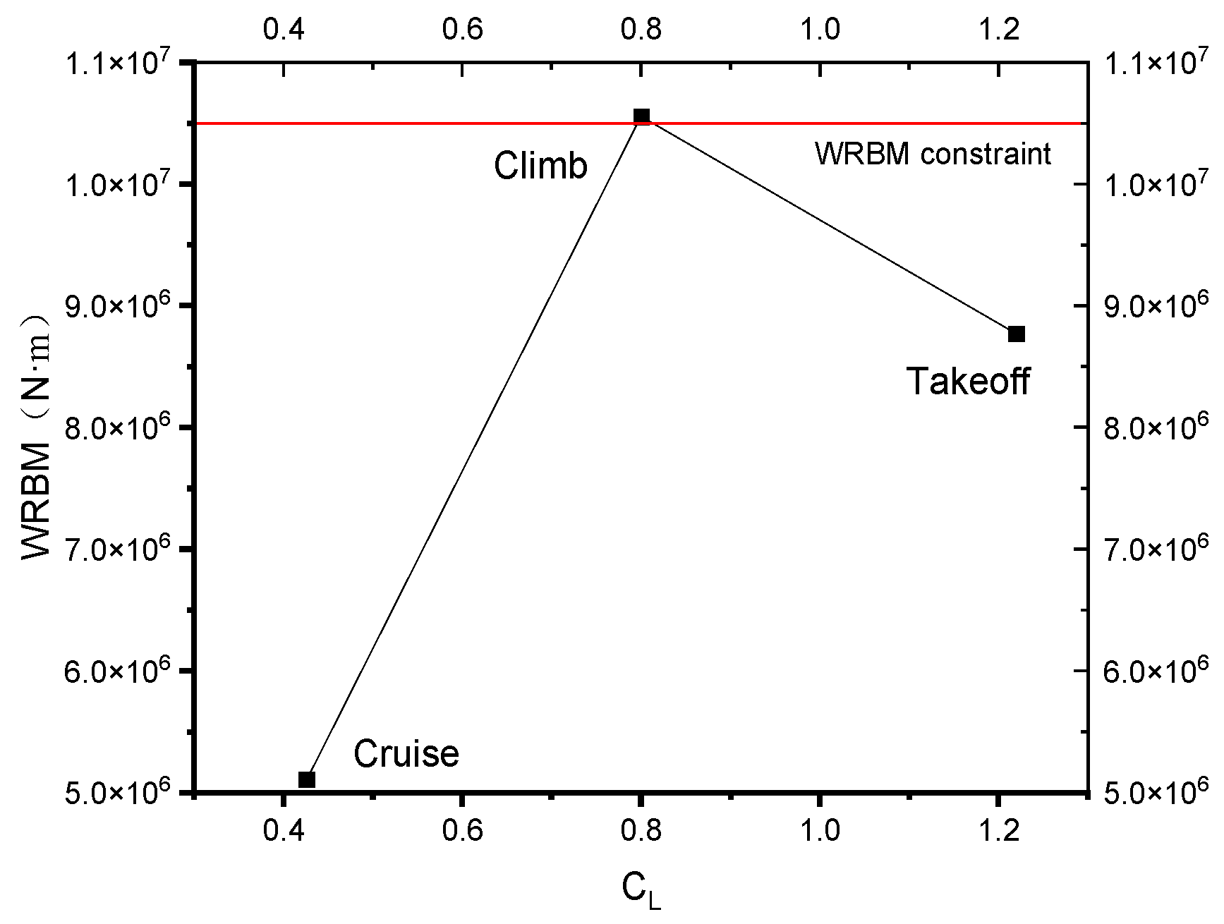
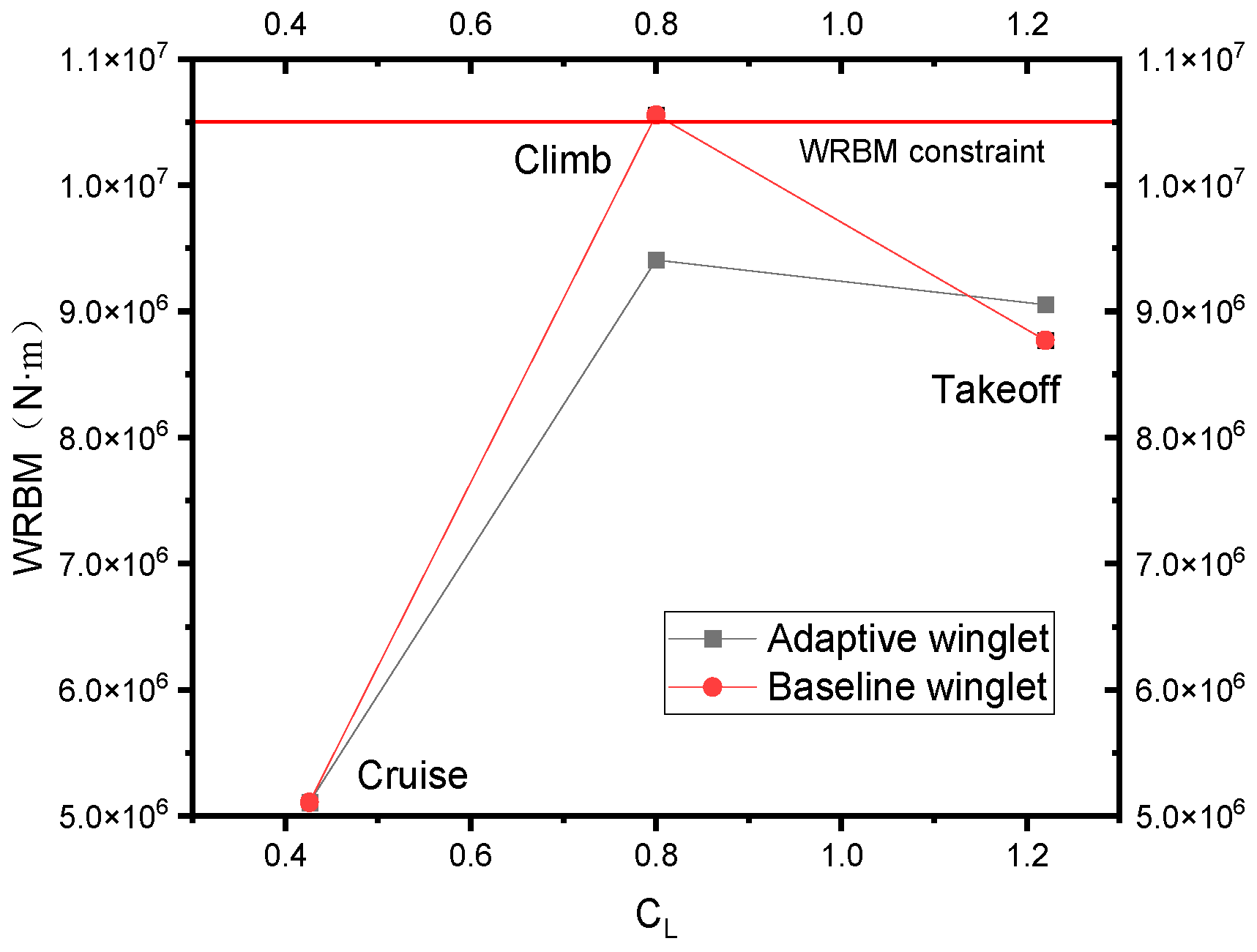
Figure 9 shows the variation in wing root bending moment for the KC-135 baseline winglet configuration under takeoff, climb, and cruise conditions. The results demonstrate that wing root bending moment increases significantly during low-speed, high-lift phases, particularly during takeoff and climb, where aerodynamic loads are elevated. The maximum wing root bending moment of the baseline winglet configuration is observed during the climb phase, reaching 1.05 × 10⁷ N·m. According to Boeing technical reports, the baseline winglet of the KC-135 aircraft was designed under a structural constraint that limited the increase in wing root bending moment relative to the clean wing configuration to within approximately 3%. To ensure structural feasibility and to introduce a conservative safety margin, the present study adopts the maximum WRBM of the baseline winglet as the reference upper bound.
This constraint is explicitly enforced in the response surface–based optimization, and the resulting optimal morphing envelope is subsequently verified to satisfy the wing root bending moment limit across the entire considered range of winglet height and cant angle variations and for all relevant flight phases.

3.4. Response Surface Optimization of Key Parameters Under Different Flight Phases

This study treats the winglet height and cant angle as design variables, with the drag coefficient and wing root bending moment taken as response quantities. A two-factor, two-level response surface methodology design of experiments is employed. Subject to the wing-root bending moment constraint, the optimal combinations of winglet height and cant angle for the takeoff and climb phases are obtained by minimizing the drag coefficient. It should be noted that the baseline winglet was optimized for the cruise condition. Therefore, its existing geometric parameters (height = 0.135b/2, cant angle = 20°) can be regarded as the baseline optimal solution for the cruise phase. A detailed description of the response surface model construction and optimization procedure is provided in Appendix B, while only the final optimization results are presented here.

3.4.1. Optimal Values of the Winglet’s Height and Cant Angle During the Takeoff Phase

Regression analysis of the experimental results is performed to derive the response surface equations for the CD and wing root bending moment during the takeoff phase, as shown in Equations (7) and (8). The analysis of variance (ANOVA) results presented in Table A5 and Table A6 of Appendix B indicate that the R2, adjusted R2, and predicted R2 values of both response surface models all exceed 90% and are in close agreement. This consistency demonstrates a good quality of fit and confirms that the models possess statistically significant predictive accuracy.
C D = 0.158705 0.000086 X 5 0.1033 X 4 + 0.000001 X 5 2 + 0.2163 X 4 2 0.000433 X 5 × X 4
W R B M = 8624894 + 6515 X 5 1416896 X 4 61.99 X 5 2 + 9229545 X 4 2 + 36783 X 5 × X 4
Based on the analysis of variance results, the relative contributions of the design variables to the responses were further quantified using the adjusted SS. For the drag coefficient during the takeoff phase, height is identified as the dominant factor, accounting for 56.38% of the total model variance, while cant angle contributes 31.38%. In contrast, the wing root bending moment exhibits a different sensitivity trend, with cant angle playing a more significant role and contributing 59.63% of the total variance, compared with 27.14% for height, as shown in Table 6. These results suggest that, during takeoff, height variation should be prioritized when the primary objective is drag reduction, whereas cant angle adjustment is more effective for controlling the wing root bending moment. The distinct sensitivity characteristics of CD and wing root bending moment to winglet geometry indicate that no single parameter can simultaneously dominate both objectives. Therefore, a coordinated morphing mode involving both height and cant angle is required, providing a clear basis for determining the optimal morphing mode and morphing envelope in the subsequent analysis.
Solving Equations (7) and (8) for the three morphing modes of adaptive winglets separately, the optimal values of winglet height and cant angle are defined as follows:
(1)
Height morphing mode: Since the adaptive winglet is based on the original KC-135 winglet, its initial cant angle is 20°, and its initial height is 0.135b/2. In the height morphing mode, the cant angle remains constant at 20°. Substituting the cant angle (X5 = 20°) into Equations (7) and (8), the optimal height during the takeoff phase is calculated to be 0.2b/2.
(2)
Cant Angle morphing mode: The height of the winglet remains at its initial value of 0.135b/2. Substituting the height (X4 = 0.135) into Equations (7) and (8), the optimal cant angle during the takeoff phase is calculated to be 72.2°
(3)
Combined morphing mode: This study employed MATLAB’s Sequential Quadratic Programming (SQP) algorithm to determine the optimal height and cant angle. Sequential quadratic programming is a powerful optimization algorithm commonly used to solve nonlinear optimization problems with constraints. The optimal height (X4 = 0.2) and cant angle (X5 = 86.3°) during the takeoff phase are obtained.

3.4.2. Optimal Values of the Winglet’s Height and Cant Angle During the Climb Phase

The response surface equations for the CD and wing root bending moment at the climb phase are shown in Equations (9) and (10). The R2, adjusted R2, and predicted R2 values of both response surface models all exceed 90% and are in close agreement, as shown in Table A8 and Table A9 of Appendix B.
C D = 0.068084 0.000028 X 5 0.07877 X 4 + 0.1899 X 4 2 0.000312 X 5 × X 4
W R B M = 10003740 + 9578 X 5 + 2664263 X 4 96.1 X 5 2 3477970 X 4 2 + 59964 X 5 × X 4
The contributions of variables to the responses during the climb phase is listed in Table 7. A consistent sensitivity pattern can be observed across the takeoff and climb phases. For both flight conditions, height is identified as the dominant parameter influencing the drag coefficient, whereas cant angle plays a more significant role in governing the wing root bending moment. This indicates that drag reduction during low-speed flight phases is primarily driven by variations in winglet height, while structural load control is more sensitive to cant angle adjustment.
Solve Equations (9) and (10) for the three morphing modes of adaptive winglets separately. The optimal cant angle in cant angle morphing mode is 15.8°, the optimal height in height morphing mode is 0.115b/2, and the optimal height and cant angle in combined morphing mode are 0.192b/2 and 8.2°, respectively.

3.5. Optimal Morphing Envelope of Adaptive Winglet

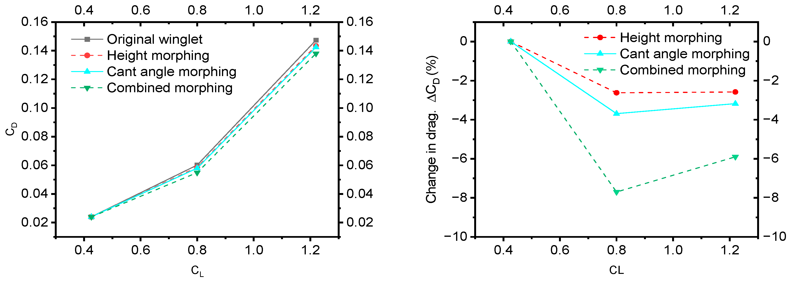
Figure 10 compares the drag reduction performance of the three winglet morphing modes relative to the original fixed winglet. The left panel illustrates the variation in the drag coefficient with lift coefficient for the original configuration and the morphing cases, while the right panel presents the corresponding percentage change in drag (ΔCD) achieved by each morphing mode.
As shown in the left panel, all morphing modes reduce the drag coefficient compared with the original winglet across the entire range of lift coefficient, with the combined morphing mode consistently yielding the lowest drag coefficient. This indicates that the adaptive winglet provides an additional aerodynamic benefit beyond that of a fixed geometry. The quantitative drag reduction efficiencies are further highlighted in the right panel. Among the three morphing modes, the height morphing mode exhibits the smallest improvement, with a maximum drag reduction of approximately 2.7%. The cant angle morphing mode performs moderately better, achieving maximum drag reductions of 3.7%. In contrast, the combined morphing mode delivers a substantially higher drag reduction, reaching up to 8.8%, which is more than twice that achieved by single-parameter morphing. This result demonstrates the strong synergistic effect between winglet height and cant angle, confirming that multi-degree-of-freedom morphing is significantly more effective for drag reduction than individual parameter adjustments.
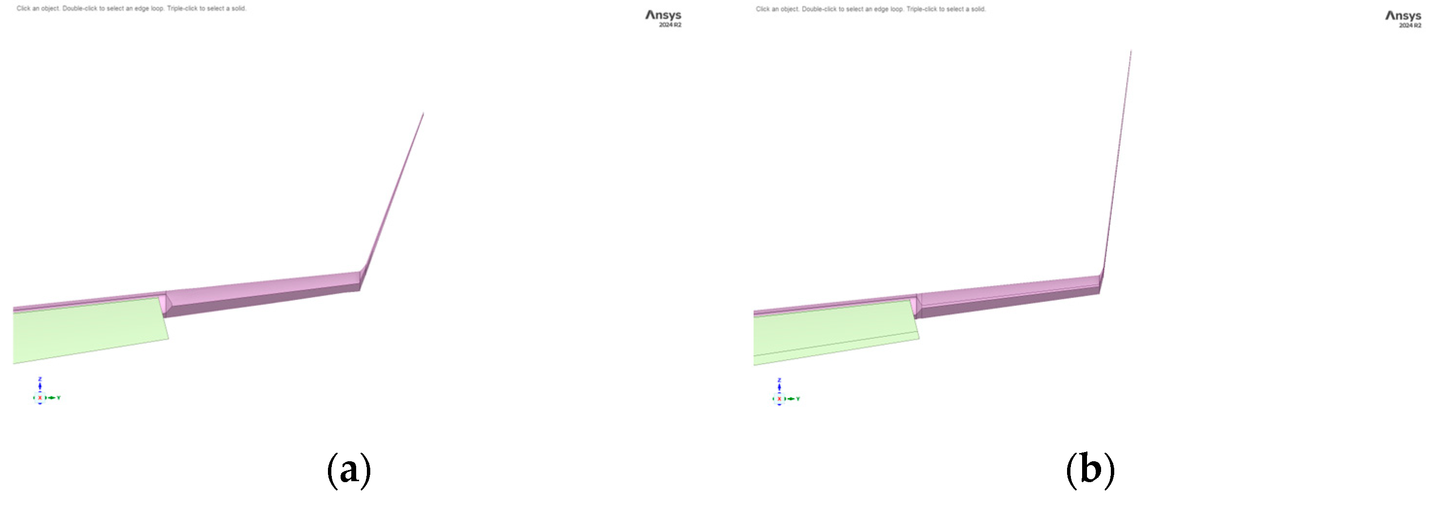
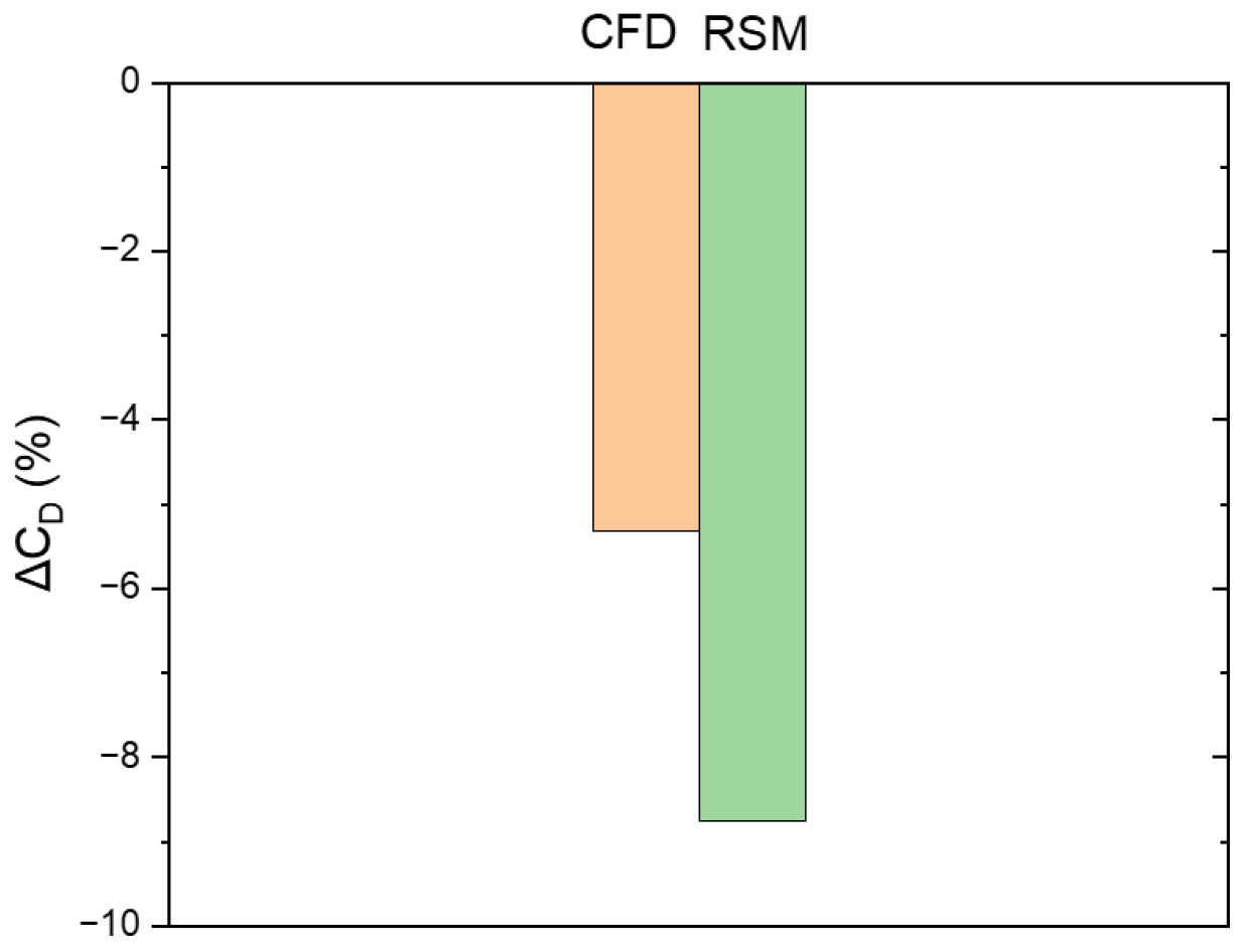
A CFD-based cross-validation was performed to evaluate the aerodynamic performance of the morphing winglet configurations at climb phases, in comparison with the original baseline winglet. The optimized morphing geometries were reconstructed in the CFD model, and the corresponding drag coefficient were computed under identical flow and boundary conditions, as shown in Figure 11. The CFD results confirm that the adapive winglet maintains a consistent drag reduction trend relative to the baseline configuration at climb phases, demonstrating effective drag control under realistic operating conditions, as shown in Figure 12. These findings provide independent numerical validation of the response surface predictions and indicate that the aerodynamic benefits of the proposed morphing strategy are not limited to the surrogate model but are also preserved in CFD simulations.
In addition, the variation in the wing root bending moment was evaluated throughout the entire morphing process of the adaptive winglet, and the corresponding results are illustrated in the accompanying Figure 13. The wing root bending moment remains consistently within the predefined constraint limits for all morphing configurations. This indicates that the proposed winglet morphing strategies do not induce excessive structural loads and that the structural safety of the wing is effectively maintained throughout the deformation process.
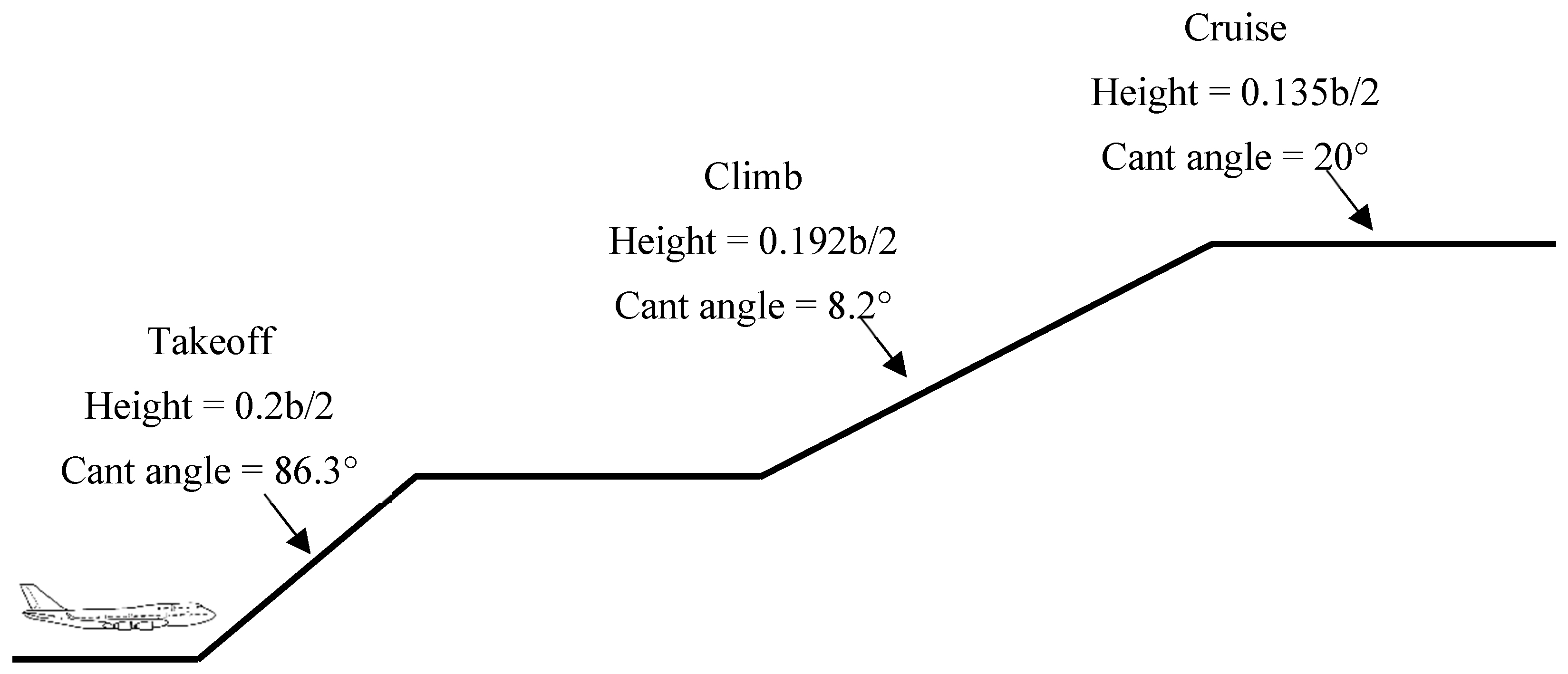
Based on the above analyses, it is evident that the combined morphing mode represents the most effective for drag reduction across different flight phases; meanwhile, it can control the root bending moment of the wing and reduce the structural load. Take the KC-135 aircraft for example, the optimal morphing envelope of the winglet is summarized in Figure 14, which illustrates the phase-dependent variations in the optimal winglet height and cant angle during takeoff, climb, and cruise.
To further substantiate the practical significance of the observed aerodynamic improvements, a mission-level benefit assessment is performed based on a simplified performance integration. Rather than relying solely on instantaneous drag reduction values, the potential fuel savings are estimated using a representative short-range mission profile. For a typical 1000 km mission of a representative narrow-body regional aircraft, the climb phase accounts for approximately 25% of the total fuel consumption. Assuming an average drag reduction of 8% during the climb segment, the corresponding fuel flow reduction is approximated to scale proportionally with drag. Under these assumptions, the estimated fuel saving amounts to approximately 60 kg per flight. When extrapolated to a conservative annual utilization of 200 flights, this corresponds to an annual fuel saving of about 12 tons per aircraft. Using a standard aviation fuel emission factor of 3.16 kg CO2 per kg of fuel, the associated reduction in CO2 emissions is approximately 38 tons per year. At a representative fuel price of 0.8 USD/kg, this translates into an annual operating cost reduction of roughly 9600 USD per aircraft. Although this analysis is based on simplified assumptions and intended as an order-of-magnitude estimate, it demonstrates that the aerodynamic benefits predicted by the present study can translate into meaningful mission-level performance gains. These results provide additional validation of the practical relevance of the proposed adaptive winglet concept beyond instantaneous aerodynamic metrics.

4. Discussion

This study presents an engineering-oriented framework for adaptive winglet design that aims to identify both the optimal morphing mode and its feasible morphing envelope across multiple flight phases. By integrating Plackett–Burman parameter screening with response surface methodology, the proposed approach enables an efficient reduction in the design space and a systematic assessment of morphing modes under combined aerodynamic and structural considerations.
The screening results indicate that winglet height and cant angle are the dominant geometric parameters influencing induced drag among the variables considered. Based on this finding, three representative morphing modes—height morphing, cant angle morphing, and combined morphing—are defined and evaluated in subsequent optimization analyses. The response surface results reveal a consistent sensitivity trend during the takeoff and climb phases. Winglet height primarily governs drag reduction, whereas cant angle exerts a stronger influence on the wing root bending moment. This distinction indicates that aerodynamic efficiency improvement and structural load control are driven by different geometric mechanisms. From an engineering perspective, drag reduction during these phases should therefore prioritize adjustments in winglet height, while cant angle variations are more effective for managing bending moment constraints. As a result, a single-parameter morphing mode is insufficient to achieve a balanced optimization of aerodynamic and structural objectives.
Among the evaluated morphing modes, the combined morphing of winglet height and cant angle exhibits a clear synergistic effect and delivers the best overall performance. Compared with the baseline fixed winglet configuration, the combined morphing mode achieves a maximum drag reduction of up to 8.8% while satisfying the wing root bending moment constraint. By synthesizing the optimal solutions obtained for takeoff, climb, and cruise conditions, a practical morphing envelope is established, providing quantitative guidance for adaptive winglet implementation throughout the flight profile.

5. Conclusions

Overall, the proposed framework offers a systematic and computationally efficient tool for preliminary and conceptual adaptive winglet design, supporting morphing mode selection and aerodynamic performance trade-off analysis. The present study primarily focuses on aerodynamic performance, with wing root bending moment introduced as a first-order structural proxy to constrain the design space at an early design stage, rather than as a comprehensive assessment of structural or aeroelastic feasibility. The resulting morphing envelope is therefore intended to represent a feasible conceptual design range, potentially implemented as discrete, phase-dependent configurations rather than continuous in-flight morphing.
Future work will extend the proposed framework to incorporate detailed structural stiffness modeling, actuator force and hinge load estimation, aeroelastic stability and flutter analysis, as well as experimental validation, in order to further refine and validate the proposed morphing envelope.

Author Contributions

Conceptualization, W.L.; methodology, W.L.; software, W.L.; validation, W.L.; formal analysis, W.L.; investigation, W.L.; resources, W.L.; data curation, W.L.; writing—original draft preparation, W.L.; writing—review and editing, B.K.S.W.; visualization, W.L.; supervision, D.W. All authors have read and agreed to the published version of the manuscript.

Funding

This research received no external funding.

Institutional Review Board Statement

Not applicable.

Data Availability Statement

Data will be made available on request.

Conflicts of Interest

The authors declare no conflicts of interest.

Abbreviations

The following abbreviations are used in this manuscript:
PBPlackett–Burman (Design)
RSMResponse Surface Methodology
VLMVortex Lattice Method
ANOVAAnalysis of Variance
WRBMWing Root Bending Moment
SQPSequential Quadratic Programming
CFDComputational Fluid Dynamics
UAVUnmanned Aerial Vehicle
CLLift coefficient
CDDrag coefficient
SSSums of squares
DFDegrees of Freedom
MSMean Squares
MSRMean Square Regression
MSEMean Square Error
SStandard Error of the Regression
RCoefficient of Determination

Appendix A

Commercial statistical software (Minitab Version 17) was employed solely as a convenient implementation of standard DOE, ANOVA, and response surface methodology procedures. All experimental designs and statistical analyses follow well-established formulations and can be readily reproduced using alternative statistical platforms (e.g., MATLAB, Python, or R) based on the information provided. The Plackett–Burman screening design was generated using Minitab, which applies randomization to the run order by default. This randomization minimizes the potential influence of systematic numerical or modeling biases on the estimated main effects. No blocking was introduced in the design, as all numerical experiments were conducted under identical computational settings and solver configurations. Consequently, no known nuisance factors were present that would require blocking.
The data in Table A1 were analyzed, yielding the regression coefficients and their significance for each factor, as shown in Table A2 The definitions of terms used in Table A2 are as follows:
  • The DF (Degrees of Freedom) represents the number of independent values that can vary in calculating a statistic.
  • The Adj SS (Adjusted Sums of Squares) are measures of variation for different model components.
  • The Adj MS (Adjusted Mean Squares) is defined as Adj SS divided by the DF.
    A d j   M S = A d j S S D F
  • The F-value is the test statistic used to determine whether the term is associated with the response. It is the ratio of the mean square for regression to the mean square for error.
    F = M S R M S E
    where MSR = Mean Square Regression, MSE = Mean Square Error.
  • The p-value is a probability that measures the evidence against the null hypothesis. Lower probabilities provide more substantial evidence against the null hypothesis. To determine whether the model explains variation in the response, compare the p-value for the model to your significance level to assess the null hypothesis. The null hypothesis for the overall regression is that the model does not explain any variation in the response. Usually, a significance level (denoted as α or alpha) of 0.05 works well. A significance level of 0.05 indicates a 5% risk of concluding that the model explains variation in the response when the model does not.
  • The S (Standard Error of the Regression) measures the average distance the observed values fall from the regression line. A smaller S indicates a better fit.
  • The R2 (Coefficient of Determination) represents the proportion of the variance in the response variable explained by the predictors.
  • Adjusts R2 for the number of predictors in the model, preventing overestimating the model’s explanatory power when adding unnecessary predictors.
  • Predicted R2 measures how well the model predicts new observations. A high predicted R2 indicates good predictive performance.

Table A1. The Plackett–Burman design result.
NX1X2/degX3X4/mX5/degX6/degX7/degCD
10.6140.150.291.40−50.020126
21600.150.20−5−50.023634
31140.680.070−500.023588
41600.680.0791.40−50.022778
50.6600.680.0791.4−5−50.022989
60.6600.150.070000.023436
70.6600.680.20000.023351
81140.680.200−50.023626
91140.150.0791.4000.022702
100.6140.680.291.4−500.020402
110.6140.150.070−5−50.023475
121600.150.291.4−500.021289
Table A2. Analysis of Variance.
SourceDFAdj SSAdj MSF-Valuep-Value
Model70.0000160.0000025.480.06
Linear70.0000160.0000025.480.06
Root chord10.0000010.0000012.890.164
Sweep angle/deg10.0000010.0000012.490.19
Taper ratio1000.840.41
Hight/m10.0000040.0000048.40.044
Cant angle/deg10.000010.00001230.009
Toe angle/deg1000.080.79
Twist angle/deg1000.680.456
Error40.0000020
Total110.000018
S0.0006514
R290.56%
Adjusted R274.05%
Predicted R215.08%
Table A2 shows that the regression model is not statistically significant because the p-value exceeds 0.05. Since the toe angle has the highest p-value of 0.79, it should be removed from the model. A new regression analysis should be conducted without the toe angle variable, and the results are shown in Table A3. The regression model’s p-value was below 0.05, indicating that it is statistically significant.
Table A3. Analysis of Variance after toe angle was excluded.
SourceDFAdj SSAdj MSF-Valuep-Value
Model60.0000160.0000037.820.020
Linear60.0000160.0000037.820.020
Root chord10.0000010.0000013.540.118
Sweep angle/deg10.0000010.0000013.050.141
Taper ratio1001.040.356
Hight/m10.0000040.00000410.300.024
Cant angle/deg10.000010.0000128.190.003
Twist angle/deg1000.830.403
Error50.0000020
Total110.000018
S0.0005885
R290.37%
Adjusted R278.82%
Predicted R244.55%
As mentioned above, Minitab software offers powerful visualization tools for data analysis. The Pareto charts are commonly used to compare the statistical significance of different factors visually. Minitab plots the Pareto charts of the factors’ absolute values in descending order. The red vertical line in the chart is drawn based on a p-value of 0.05. It can be considered statistically significant only if a factor’s bar extends beyond the red line.

Appendix B

Using Minitab software to perform response surface design, 13 experiments are required for two factors at two levels. Winglets with different combinations of height and cant angle generate the experimental matrix. The CD and wing root bending moment of the wing are calculated at the conditions of Ma = 0.3 and CL = 1.22. The results are shown in Table A4. Replication was introduced through repeated evaluations at the center point of the response surface design. As shown in Table A4 and Table A7, five identical center-point runs were performed, enabling direct estimation of pure error and assessment of numerical repeatability. The uncertainty of the estimated effects is quantified through the residual variance obtained from replicated center points. Based on the standard error of regression and the corresponding error degrees of freedom, 95% confidence intervals for the main and interaction effects can be established following standard RSM procedures.
Table A4. Response surface methodology experimental matrix at the takeoff phase.
NX5/degX4/mCDWRBM
10.00.0700.1521818, 581, 139
291.40.0700.1487388, 908, 170
30.00.2000.1468268, 678, 241
491.40.2000.1382439, 442, 323
50.00.1350.1489078, 624, 072
691.40.1350.1421359, 127, 314
745.70.0700.1493868, 822, 355
845.70.2000.1400029, 265, 958
945.70.1350.1438388, 993, 805
1045.70.1350.1438398, 993, 650
1145.70.1350.1438388, 993, 783
1245.70.1350.1438378, 993, 747
1345.70.1350.1438388, 993, 795
Table A5. Analysis of variance for CD at takeoff phase.
SourceDFAdj SSAdj MSF-Valuep-Value
Model50.0001880.000038288.50
Linear20.0001650.0000836330
Cant angle/deg10.0000590.000059451.790
Height/m10.0001060.000106814.210
Square20.0000160.00000862.930
Cant angle × Cant angle10.0000080.00000864.210
Height × Height10.0000020.00000217.70.004
2-Way Interaction10.0000070.00000750.650
Cant angle × Height10.0000070.00000750.650
Error70.0000010
Lack-of-Fit30.0000010721,3590
Pure Error400
Total120.000189
S0.0003610
R299.52%
Adjusted R299.17%
Predicted R295.10%
Table A6. Analysis of variance for wing root bending moment at takeoff phase.
SourceDFAdj SSAdj MSF-Valuep-Value
Model57.11 × 10111.42 × 1011154.460
Linear26.16 × 10113.08 × 1011334.850
Cant angle/deg14.24 × 10114.24 × 1011460.430
Height/m11.93 × 10111.93 × 1011209.270
Square24.66 × 10102.33 × 101025.340.001
Cant angle × Cant angle14.63 × 10104.63 × 101050.310
Height × Height14.2 × 1094.2 × 1094.560.07
2-Way Interaction14.78 × 10104.78 × 101051.90
Cant angle × Height14.78 × 10104.78 × 101051.90
Error76.44 × 1099.2 × 108
Lack-of-Fit36.44 × 1092.15 × 109536,877.40
Pure Error415,9963999
Total127.17 × 1011
S30,333.7
R299.10%
Adjusted R298.46%
Predicted R291.04%
Table A7. Response surface methodology experimental matrix at climb phase.
NX5/degX4/mCDWRBM
10.00.0700.06333610, 203, 839
291.40.0700.06188010, 662, 090
30.00.2000.06007310, 366, 393
491.40.2000.05491411, 537, 141
50.00.1350.06092410, 300, 466
691.40.1350.05762111, 108, 532
745.70.0700.06231810, 538, 553
845.70.2000.05626711, 242, 524
945.70.1350.05846610, 907, 649
1045.70.1350.05846910, 907, 548
1145.70.1350.05846910, 907, 552
1245.70.1350.05846710, 907, 729
1345.70.1350.05847010, 907, 639
Table A8. Analysis of variance for CD at climb phase.
SourceDFAdj SSAdj MSF-Valuep-Value
Model50.000070.000014331.590
Linear20.0000610.00003721.460
Cant angle/deg10.0000160.000016390.550
Height/m10.0000440.0000441052.380
Square20.0000060.00000366.670
Cant angle × Cant angle10.0000020.00000240.210
Height × Height10.0000020.00000242.340
2-Way Interaction10.0000030.00000381.660
Cant angle × Height10.0000030.00000381.660
Error700
Lack-of-Fit30050,276.080
Pure Error400
Total120.00007
S0.0002049
R299.58%
Adjusted R299.28%
Predicted R295.73%
Table A9. Analysis of variance for wing root bending moment at climb phase.
SourceDFAdj SSAdj MSF-Valuep-Value
Model51.76 × 10123.52 × 1011215.060
Linear21.50 × 10127.48 × 1011456.710
Cant angle/deg19.90 × 10119.90 × 1011604.640
Height/m15.06 × 10115.06 × 1011308.780
Square21.38 × 10116.91 × 101042.190
Cant angle × Cant angle11.11 × 10111.11 × 101167.980
Height × Height15.96 × 1085.96 × 1080.360.565
2-Way Interaction11.27 × 10111.27 × 101177.520
Cant angle × Height11.27 × 10111.27 × 101177.520
Error71.15 × 10101.64 × 109
Lack-of-Fit31.15 × 10103.82 × 109672,307.30
Pure Error422,7285682
Total121.77 × 1012
S40,461.6
R299.35%
Adjusted R298.89%
Predicted R293.42%

Appendix C. CFD Mesh and Solver Settings

CFD were performed using a Reynolds-averaged Navier–Stokes (RANS) framework to cross-validate the OpenVSP results. The computational domain consisted of a far-field enclosure extending 10 chord lengths upstream, downstream, and in the spanwise directions to minimize boundary effects. An unstructured mesh was employed. The total cell count ranged from approximately 0.8 to 1.7 million, depending on the specific winglet configuration and morphing state. Near-wall mesh refinement was applied to ensure adequate resolution for turbulence modeling. A mesh independence study was conducted by systematically refining the grid until variations in the lift and drag coefficients were below 2%, confirming numerical robustness.
A pressure-based transient solver was employed. Turbulence effects were modeled using the k–ω SST turbulence model, selected for its proven capability in capturing adverse pressure gradients and wing–winglet junction flows. Air was treated as an incompressible, Newtonian fluid, consistent with the low Mach number regime of the investigated flight conditions. Second-order spatial discretization schemes were applied to all governing equations to reduce numerical diffusion. Pressure–velocity coupling was handled using a coupled algorithm. Velocity inlet and pressure outlet boundary conditions were prescribed at the far-field boundaries, corresponding to the freestream conditions of the investigated flight phases. No-slip wall boundary conditions were applied to all solid surfaces. Convergence was considered achieved when the normalized residuals of all governing equations decreased below 10−5, and the integrated aerodynamic forces (lift and drag) exhibited negligible variation with further iterations.
The wing and winglet model in OpenVSP was discretized using a 62 × 40 surface mesh. VSPAERO was employed to compute the lift and drag coefficients, utilizing the Vortex Lattice Method (VLM) as the underlying aerodynamic solver, with the Kármán–Tsien compressibility correction enabled.

References

  1. Yohanes, A.; Irwansyah, R. Modification of Wingtip Devices Configuration to Increase Aerodynamic Efficiency of Aircraft. J. Phys. Conf. Ser. 2025, 3103, 012019. [Google Scholar] [CrossRef]
  2. Maughmer, M.D. Design of Winglets for High-Performance Sailplanes. J. Aircr. 2003, 40, 1099–1106. [Google Scholar] [CrossRef]
  3. Wang, W.; Yuan, G. Review on the Structure Design of Morphing Winglets. Aerospace 2024, 11, 1004. [Google Scholar] [CrossRef]
  4. Li, B.; Zhang, Z.; Jia, F.; Sun, J.; Liu, Y.; Leng, J. Research status and development trend of morphing wingtip technology. Acta Aeronaut. Astronaut. Sin. 2024, 45, 30042. [Google Scholar] [CrossRef]
  5. Barbarino, S.; Bilgen, O.; Ajaj, R.M.; Friswell, M.I.; Inman, D.J. A Review of Morphing Aircraft. J. Intell. Mater. Syst. Struct. 2011, 22, 823–877. [Google Scholar] [CrossRef]
  6. Vasista, S.; Tong, L.; Wong, K.C. Realization of Morphing Wings: A Multidisciplinary Challenge. J. Aircr. 2012, 49, 11–28. [Google Scholar] [CrossRef]
  7. Meyer, P. In-Flight Folding Wingtips. In Pressure-Actuated Cellular Structures for Adaptive Wingtips; Springer Nature: Cham, Switzerland, 2025; pp. 9–26. [Google Scholar]
  8. Ursache, N.; Melin, T.; Isikveren, A.; Friswell, M. Morphing winglets for aircraft multi-phase improvement. In Proceedings of the 7th AIAAAviation Technology, Integration and Operation (ATIO) Conference, Belfast, Ireland, 18–20 September 2007; AIAA: Reston, VA, USA, 2012; p. 7813. [Google Scholar]
  9. Guerrero, J.E.; Sanguineti, M.; Wittkowski, K. Variable cant angle winglets for improvement of aircraft flight performance. Meccanica 2020, 55, 1917–1947. [Google Scholar] [CrossRef]
  10. Zhang, L.; Ma, D.L.; Yang, M.Q.; Wang, S.Q. Optimization and analysis of winglet configuration for solar aircraft. Chin. J. Aeronaut. 2020, 33, 3238–3252. [Google Scholar] [CrossRef]
  11. Rajabi, M.; Jahangirian, A. Design optimization of a morphing winglet for all flight missions of a civil aircraft. Proc. Inst. Mech. Eng. Part G J. Aerosp. Eng. 2024, 239, 09544100241287653. [Google Scholar] [CrossRef]
  12. Segui, M.; Abel, F.R.; Botez, R.M.; Ceruti, A. New Aerodynamic Studies of an Adaptive Winglet Application on the Regional Jet CRJ700. Biomimetics 2021, 6, 54. [Google Scholar] [CrossRef]
  13. Meyran, P.; Pain, H.; Botez, R.M.; Laliberté, J.J.I.B. Morphing winglet design for aerodynamic performance optimization of the CRJ-700 Aircraft. Part 1-Structural design. INCAS Bull. 2021, 13, 113–128. [Google Scholar] [CrossRef]
  14. Panagiotou, P.; Antoniou, S.; Yakinthos, K. Cant angle morphing winglets investigation for the enhancement of the aerodynamic, stability and performance characteristics of a tactical Blended-Wing-Body UAV. Aerosp. Sci. Technol. 2022, 123, 107467. [Google Scholar] [CrossRef]
  15. Bourdin, P.; Gatto, A.; Friswell, M.I. Aircraft Control via Variable Cant-Angle Winglets. J. Aircr. 2008, 45, 414–423. [Google Scholar] [CrossRef]
  16. Gatto, A.; Mattioni, F.; Friswell, M.I. Experimental Investigation of Bistable Winglets to Enhance Aircraft Wing Lift Takeoff Capability. J. Aircr. 2009, 46, 647–655. [Google Scholar] [CrossRef]
  17. Wang, C.; Khodaparast, H.H.; Friswell, M.I. Conceptual study of a morphing winglet based on unsymmetrical stiffness. Aerosp. Sci. Technol. 2016, 58, 546–558. [Google Scholar] [CrossRef]
  18. Kaygan, E.; Gatto, A.J.I.J.o.A.; Engineering, M. Investigation of adaptable winglets for improved UAV control and performance. Int. J. Mech. Aerosp. Ind. Mechatron. Eng. 2014, 8, 1289–1294. [Google Scholar]
  19. Zhang, W.; Zhang, C.; Liu, B.; Zhang, B.; Wang, L. Research on Variable Sweepback Angle of Winglet Driven by Shape Memory Alloy. IOP Conf. Ser. Mater. Sci. Eng. 2020, 926, 012014. [Google Scholar] [CrossRef]
  20. Kaygan, E.; Gatto, A.J.I.J.o.A.; Engineering, M. Computational Analysis of Adaptable Winglets for Improved Morphing Aircraft Performance. Int. J. Mech. Aerosp. Ind. Mechatron. Manuf. Eng. 2015, 9, 1205–1211. [Google Scholar]
  21. Falcão, L.; Gomes, A.A.; Suleman, A. Aero-structural Design Optimization of a Morphing Wingtip. J. Intell. Mater. Syst. Struct. 2011, 22, 1113–1124. [Google Scholar] [CrossRef]
  22. Daniele, E.; De Fenza, A.; Vecchia, P.D. Conceptual adaptive wing-tip design for pollution reductions. J. Intell. Mater. Syst. Struct. 2012, 23, 1197–1212. [Google Scholar] [CrossRef]
  23. Eguea, J.P.; Bravo-Mosquera, P.D.; Catalano, F.M. Camber morphing winglet influence on aircraft drag breakdown and tip vortex structure. Aerosp. Sci. Technol. 2021, 119, 107148. [Google Scholar] [CrossRef]
  24. Eguea, J.P.; Pereira Gouveia da Silva, G.; Martini Catalano, F. Fuel efficiency improvement on a business jet using a camber morphing winglet concept. Aerosp. Sci. Technol. 2020, 96, 105542. [Google Scholar] [CrossRef]
  25. Dimino, I.; Gallorini, F.; Palmieri, M.; Pispola, G. Electromechanical Actuation for Morphing Winglets. Actuators 2019, 8, 42. [Google Scholar] [CrossRef]
  26. Ishimitsu, K.; Zanton, D. Boeing commercial airplane co seattle wa. In Design and Analysis of Winglets for Military Aircraft. Phase 2; DTIC: Fort Belvoir, VA, USA, 1977. [Google Scholar]
  27. Mariën, F. Software Testing: VSPAERO; Aircraft Design and Systems Group (AERO), Department of Automotive and Aeronautical Engineering, Hamburg University of Applied Sciences: Hamburg, Germany, 2021. [Google Scholar] [CrossRef]
  28. Tsien, H.S. Similarity laws of hypersonic flows. J. Math. 1946, 25, 247–251. [Google Scholar] [CrossRef]
  29. Plackett, R.L.; Burman, J.P. The Design of Optimum Multifactorial Experiments. Biometrika 1946, 33, 305–325. [Google Scholar] [CrossRef]
  30. Box, G.E.P.; Hunter, J.S. Multi-Factor Experimental Designs for Exploring Response Surfaces. Ann. Math. Stat. 1957, 28, 195–241. [Google Scholar] [CrossRef]
  31. Houghton, E.L.; Carpenter, P.W. Aerodynamics for Engineering Students; Elsevier: Amsterdam, The Netherlands, 2003. [Google Scholar]
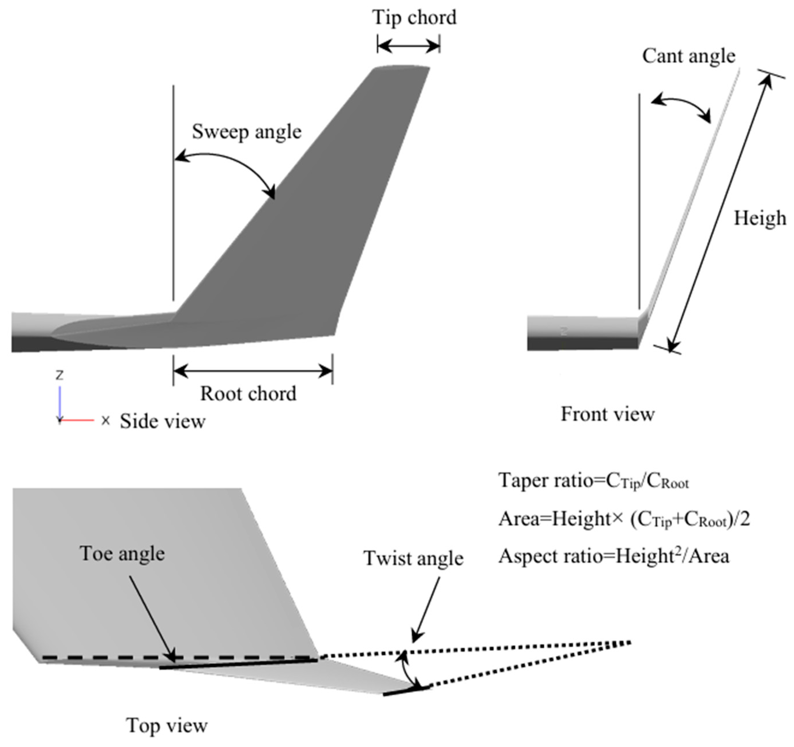
Figure 1. Schematic diagram of winglet parameters.
Applsci 16 01645 g001
Figure 2. Published morphing mode of the adaptive winglet.
Applsci 16 01645 g002
Figure 3. Flowchart of this study.
Applsci 16 01645 g003
Figure 4. KC-135 wing and winglet model.
Applsci 16 01645 g004
Figure 5. Wing model with high-lift devices.
Applsci 16 01645 g005
Figure 6. CFD model with trailing-edge flap.
Applsci 16 01645 g006
Figure 7. Pareto chart.
Applsci 16 01645 g007
Figure 8. Optimal morphing mode of the adaptive winglets. (a) Height morphing; (b) Cant angle morphing; (c) Combined morphing.
Applsci 16 01645 g008
Figure 9. WRBM of KC-135 with fixed winglet during takeoff, climb, and cruise phase.
Applsci 16 01645 g009
Figure 10. Drag reduction efficiency among the three morphing modes.
Applsci 16 01645 g010
Figure 11. Configuration comparison of adaptive and baseline winglet. (a) baseline winglet; (b) adaptive winglet at climb phase.
Applsci 16 01645 g011
Figure 12. The drag reduction in the adaptive winglet in climb phase.
Applsci 16 01645 g012
Figure 13. The impact of morphing winglets on wing root bending moment.
Applsci 16 01645 g013
Figure 14. Optimal morphing envelope during takeoff, climb, and cruise.
Applsci 16 01645 g014
Table 1. Flow field boundary conditions in OpenVSP.
Flight ConditionSpeedLift Coefficient
Takeoff0.31.22
Climb0.40.8
Cruise0.780.426
Table 2. Grid convergence study results.
Mesh LevelTotal Cell CountLift CoefficientRelative Change vs. Previous Mesh (%)
Coarse5.5 × 1050.794-
Medium8.7 × 1050.8122.2%
Fine1.7 × 1060.8231.3%
Table 3. Comparison of drag change rates between configurations with and without winglets predicted by OpenVSP, Boeing reports, and CFD simulations.
Flight PhaseReferenceCLΔCD (Ref.)ΔCD (OpenVSP)Error (%)
TakeoffBoeing1.2204.1%3.5%−0.6%
ClimbRANS CFD0.8006.9%5.7%−1.2%
CruiseBoeing0.4267%8.9%1.9%
Table 4. The winglet geometric parameter range.
ParametersSerial NumberLevel
−1+1
Root chordX10.61
Sweep angle/degX214°60°
Taper ratioX30.150.68
Height/mX40.07b/20.20b/2
Cant angle/degX591.4°
Toe angle/degX6−5°
Twist angle/degX7−5°
Table 5. Significance levels of winglet geometric parameters.
Levelp-ValueParameters
Significantp < 0.05Cant angle, height
Non-significantp > 0.05Root chord, sweep angle, taper ratio, toe and twist angle
Table 6. Contributions of variables to the responses during the takeoff phase.
ResponseCant Angle ContributionHeight ContributionDominant Factor
CD31.38%56.38%Height
WRBM59.63%27.14%Cant angle
Table 7. Contributions of variables to the responses during the climb phase.
ResponseCant Angle ContributionHeight ContributionDominant Factor
CD22.86%62.86%Height
WRBM56.25%28.75%Cant angle
Disclaimer/Publisher’s Note: The statements, opinions and data contained in all publications are solely those of the individual author(s) and contributor(s) and not of MDPI and/or the editor(s). MDPI and/or the editor(s) disclaim responsibility for any injury to people or property resulting from any ideas, methods, instructions or products referred to in the content.