Risk Identification and Chaotic Synchronization Control for Spent Fuel Road Transportation Based on Complex Network Evolution Models

Abstract

To improve the safety of road transportation of Spent Nuclear Fuel (SNF), this paper proposes a novel approach for risk identification and chaotic synchronous control in SNF road transportation systems. Firstly, a dynamic risk evolution model for the road transportation of SNF is developed by analyzing the nonlinear interactions among vehicles, environmental conditions, and human factors using complex network analysis and nonlinear dynamics. Secondly, an enhanced K-shell decomposition method is applied to identify key risk nodes and assess the relative importance of different risk factors, providing a basis for targeted risk control. Finally, a chaotic synchronization control strategy based on Lyapunov stability is proposed to suppress risk divergence and restore system stability. Three targeted control schemes are evaluated by varying the control gain coefficients across the ‘Vehicle–Environment–Human’ dimensions. Simulation results indicate that the strategy prioritizing environmental and human risk control yields the fastest convergence, significantly outperforming vehicle-centric approaches. The results show that prioritizing both environmental and human-factor control is most effective for suppressing chaotic divergence. This provides a solid quantitative basis for the strategic shift from passive defense to active environmental warning, thereby significantly optimizing the dynamic risk management of the SNF transportation system.

1. Introduction

Driven by the global transition toward carbon neutrality, nuclear power has emerged as a cornerstone of national energy strategies worldwide due to its efficiency and low emissions [1,2,3,4,5,6]. However, this rapid expansion of generation capacity has inevitably accelerated the accumulation of high-level radioactive waste, specifically SNF. Consequently, As on-site spent fuel pool storage capacities at nuclear power plants approach saturation, the road transport of spent fuel to centralized interim storage facilities or reprocessing plants has become an indispensable and increasingly frequent critical step in the back-end of the nuclear fuel cycle [7,8]. Unlike the transport of conventional hazardous chemicals, spent nuclear fuel transport involves mobile sources of intense radioactivity, including radionuclides such as Cs-137 and Sr-90, as well as substantial residual heat. Its transport system exhibits extreme sensitivity to disturbances and high structural and behavioral complexity, arising from the tight coupling between vehicle dynamics, cask integrity, environmental conditions, and human decision-making. In the event of a serious traffic accident, such as a collision, rollover, or fire, the transport container may be damaged or its sealing integrity compromised. Any release of radioactive material would cause long-term and potentially irreversible harm to the surrounding environment and public health, while also likely provoking significant public anxiety and political consequences [9,10]. As a radioactive material, the safe transport of SNF has been explicitly included by the International Atomic Energy Agency (IAEA) within the five major categories of its definition of ‘nuclear safety’ (namely, safety of nuclear facilities, radiation safety, safety of radioactive waste management, and safety of radioactive material transport). Although severe accidents involving SNF transport are rare, their potential environmental and social consequences are extremely high, and even minor incidents can trigger significant public concern. China has established comprehensive regulatory frameworks and technical standards for radioactive material transport, including route planning, escort protocols, and emergency preparedness. The present work does not imply a lack of such procedures; rather, it seeks to provide a quantitative, dynamic risk analysis and control tool that can support and enhance these existing protocols, especially for long-distance, high-risk road segments.

Therefore, studying the evolution of risks in spent fuel transport systems is crucial for the safety and sustainable development of nuclear energy. A substantial body of academic work has examined risk assessment in hazardous materials transportation, using approaches such as probabilistic safety analysis, fuzzy evaluation methods, and machine learning techniques [11,12]. However, dynamic risk analysis focused specifically on the road transportation of spent nuclear fuel remains limited. From a methodological standpoint, most existing studies adopt a static framework in which risk factors such as driver fatigue, vehicle malfunction, and adverse weather are treated as independent or merely additive influences [13,14,15]. This approach neglects how these factors evolve and interact over the course of transportation. In reality, spent nuclear fuel transportation operates as an open and highly complex system when examined dynamically. Even small disturbances, such as minor road defects or momentary driver inattention, can be amplified by interactions within the system, causing sudden shifts from safe operation to accidents and demonstrating pronounced nonlinear behavior. Secondly, existing research on risk factors within the ‘vehicle–environment–human’ system predominantly employs linear coupling relationships for quantitative analysis [16], However, a systematic nonlinear dynamical analysis of these coupled subsystems in the specific context of SNF road transport has not yet been reported. As a result, static risk and traditional linear assessment models are no longer sufficient to address the safety management challenges of spent fuel transportation, which involves high levels of risk and operational complexity.

In response to these methodological limitations, to address the static limitations of traditional methods, this paper proposes a novel dynamic approach. The primary improvement lies in shifting the perspective from static probability estimation to dynamic stability control. Unlike existing models that treat risk as a fixed value, this approach models risk as a time-evolving state, allowing for the active suppression of cascading failures through chaotic synchronization. Complex networks and chaos theory provide complementary tools for analyzing complex systems. Complex network theory is well suited to describing the static structure of interactions among risk factors. It offers a way to visualize and quantify how different components or risk factors are linked, and how they depend on one another. Chaos theory, by contrast, focuses on the dynamic behavior of such systems [17]. It explains how their evolution over time can be highly sensitive to small disturbances and may become unpredictable. Together, these two perspectives form an integrated approach that has proved valuable in many fields, including financial risk management, epidemiology and industrial safety [18,19,20,21]. In a complex network model, a system is represented as a set of nodes, which denote entities such as components or risk factors, and edges, which denote the relationships or interactions between them [22]. Applying complex network theory in this context allows researchers to identify the elements involved in such accidents, classify risk event nodes such as system, equipment, personnel, environment and accident types, and study their interconnections. This, in turn, supports the design of more effective prevention and mitigation strategies. Thus, the primary objective of this study is to construct a dynamic evolution model for the SNF road transportation system and to identify the most effective control dimension for suppressing chaotic risk divergence. Firstly, a complex network association model of spent fuel transportation risk factors is constructed based on the ‘vehicle–environment–human’ multidimensional system. An enhanced K-shell algorithm is applied to accurately identify key risk nodes within the network. Secondly, chaotic dynamics theory is introduced to establish dynamic evolution equations for the transport risk system. The Lyapunov exponent is employed to validate the system’s chaotic properties, revealing the nonlinear patterns of risk evolution over time. Finally, based on Lyapunov stability theory, a synchronization control strategy is developed to stabilize the risk system. Simulation validation demonstrates the effectiveness of multi-dimensional control strategies in suppressing system divergence and achieving risk control, providing theoretical foundations for emergency management and proactive prevention in real-world spent fuel transportation.

The subsequent structure of this paper is as follows: Section 2 reviews relevant literature; Section 3 analyzes the characteristics of spent fuel transportation and constructs a dynamic risk evolution model; Section 4 verifies the chaotic properties of the system and the effectiveness of the control strategy through numerical simulation; Section 5 summarizes the conclusions regarding the SNF transportation risk system and proposes corresponding management recommendations.

2. Literature Review

For many years, probabilistic safety analysis and consequence assessment have formed the foundation of research on risks in spent fuel transportation. To quantify the complexity of transportation risks, Tao et al. [23] developed a six-dimensional indicator method covering human, vehicle, container, road, environmental, and regulatory factors. By combining event tree and fault tree methods, they systematically estimated the frequency of accidents in road transportation of spent nuclear fuel. Mheidat et al. [24] assessed the risks associated with spent fuel transport routes in Jordan and evaluated compliance along selected routes. These studies primarily treated risk as static probabilities or linear event chains, which is appropriate and computationally efficient for regulatory decision-making and routine safety assessments. However, this does not capture how transportation systems dynamically shift from safe operation to accidents in response to ongoing and evolving disturbances over time. This is precisely the dimension addressed by the complex-network-based chaotic model and synchronization control proposed in this paper.

Due to these transportation systems involving tightly coupled factors, researchers have increasingly adopted a systems perspective for risk identification. Hong et al. [25] showed that accidents more often arise from interactions among system components than from isolated failures. Building on this insight, complex network analysis has emerged as an effective approach for identifying critical sources of risk. Wang et al. [26] and He et al. [27] constructed risk networks for urban rail transit, successfully identifying critical causal risks using topological metrics such as degree centrality. However, existing network analyses predominantly focus on describing static topological structures, with limited research incorporating dynamic behaviors. In reality, a node that appears ordinary in topology (e.g., a minor mechanical defect in a vehicle) can become a super-spreader of risk under specific dynamic mechanisms, triggering cascading failures in the system.

Given the prevalence of ambiguous and uncertain information in transportation environments (such as driver mental states and sudden weather changes), traditional deterministic models are often insufficient. Marseguerra et al. [28] proposed a fuzzy reasoning modeling approach, establishing nonlinear mapping relationships between traffic flow, precipitation rates, vehicle speeds, and accident rates. This method effectively addresses challenges associated with limited data and uncertain parameters in spent fuel transportation. While fuzzy logic captures static parameter uncertainty, it does not account for the system’s dynamic memory effects. In spent fuel transport, accumulated driver fatigue or minor wear on vehicle components similarly exhibit such memory traits. Traditional fuzzy models struggle to characterize this chaotic evolution from quantitative to qualitative changes. Even if the probability of accidents caused by each risk is small, the consequences produced by multiple risk factors intertwined together are serious and the system is very unstable.

Therefore, to address the limitations of linear models, catastrophe theory and chaos theory have been introduced to explain sudden behavioral changes in complex systems. Mutation theory, as a study of the evolutionary process of a system, describes a system that can maintain its original state under the action of small perturbations in the steady state and, once subjected to a slight perturbation, quickly leaves its initial state [29]. Huang et al. [30], using a cusp catastrophe model for railway hazardous goods transportation, showed that when the trajectory of the system’s control parameters enters the bifurcation region, the system can suddenly jump from a safe state to a risky state.

Chaos theory, related to mutation theory, can be used to explore the evolutionary problems in complex risk systems. By adding a controller to the system, the system can take appropriate measures based on the controller’s data to achieve a safe and stable state [31]. Currently, research on the evolution of risk factors is mainly applied to software project risk [32], engineering and construction project risk [33], transportation project risk [34], and medical disease risk [35]. Although chaos theory has shown promise in various engineering applications, its use for active risk control in the highway transportation of spent nuclear fuel remains largely uninvestigated.

In summary, despite improvements in risk quantification achieved by methods such as PSA [23,24], fuzzy logic, and static networks, many accidents are driven by the gradual build-up of small deviations, so a key concern is how quickly the system can be restored to a stable state after it is disturbed. Thus, this paper proposes a novel method integrating complex network evolution with chaotic synchronization control, meaning the first introduction of chaotic synchronization control into the field of spent fuel transport. Different from traditional PSA methods that merely provide accident probabilities, we constructed a dynamic evolution equation for the ‘vehicle–environment–human’ integrated system, revealing its chaotic characteristics and shifting the focus from accident probability to system stability. This research enables the design of specific control laws that actively manage chaotic divergence by adjusting environmental, personnel, or vehicle parameters. The model is especially applicable to high-risk, long-distance, and strictly regulated radioactive material transportation operations. It provides decision-makers with real-time feedback to dynamically adjust control weights during transport, offering algorithmic support for SNF emergency response systems.

The subsequent structure of this paper is as follows: Section 2 analyzes the characteristics of spent fuel transportation and constructs a dynamic risk evolution model; Section 3 verifies the chaotic properties of the system and the effectiveness of the control strategy through numerical simulation; Section 4 summarizes the entire paper and proposes management recommendations.

3. Methodology

The road transportation of SNF is characterized by long-duration operations, varying environmental conditions, and strong couplings among driver behavior, vehicle status, and road environment. Small perturbations (e.g., a brief lapse of attention, minor road defects, sudden rainfall) may be amplified through feedback loops and interactions, eventually resulting in abrupt transitions from safe operation to accidents. Such phenomena cannot be captured adequately by static or purely linear models. Therefore, a dynamic nonlinear risk evolution model is required to:

(i)

Describe how risk levels in the vehicle, environment, and human subsystems co-evolve over time;

(ii)

Capture threshold effects, bifurcations, and possible chaotic behavior;

(iii)

Provide a basis for designing time-dependent control strategies that stabilize the overall system.

3.1. Modeling of SNF Transport Risk Network

The SNF transport risk system is an undirected complex network G = (V,E) where each node v ∈ V represents a distinct risk factor and each edge (v_i,v_j)∈E denotes a causal or triggering relationship indicating that the occurrence or escalation of factor ii can directly increase the likelihood or severity of factor j. The network structure is encoded by an adjacency matrix A = [a_ij], where a_ij = 1 if there is a mutual influence from v_i to v_j, and a_ij = 0 otherwise. Self-loops are not considered, so the main diagonal entries of A are zero. In this study, the identification process assumes that the causal topological structure of the risk network remains static during the transport mission. Nodes are used to abstract the various risk factors that lead to transportation accidents, and the edges between the nodes represent the accident-triggering relationships or causal dependencies between them. For instance, if a traffic accident caused by vehicle collision leads to the damage of an SNF cask, a directed edge connects the corresponding risk nodes. The expression of the adjacency matrix A of the graph G is shown below:

$$A={(a_{ij})}_{m\times n}=\left\{\begin{array}{l}1,v_i,v_j\in E,\\ 0,(v_i,v_j)\notin E.\end{array}\right.$$

(1)

where $(v_i,v_j)\in E$ denotes that there is a connected edge from node v_i to node v_j, $(v_i,v_j)\notin E$ denotes that there is no connected edge from node v_i to node v_j. The matrix form of A is shown below:

$$A=\left[\begin{array}{cccc}0& a_{12}& \dots & a_{1n}\\ a_{21}& 0& \dots & a_{2n}\\ \begin{array}{l}.\\ .\end{array}& \begin{array}{l}.\\ .\end{array}& \begin{array}{l}.\\ .\end{array}& \begin{array}{l}.\\ .\end{array}\\ a_{i1}& a_{i2}& \dots & 0\end{array}\right]$$

(2)

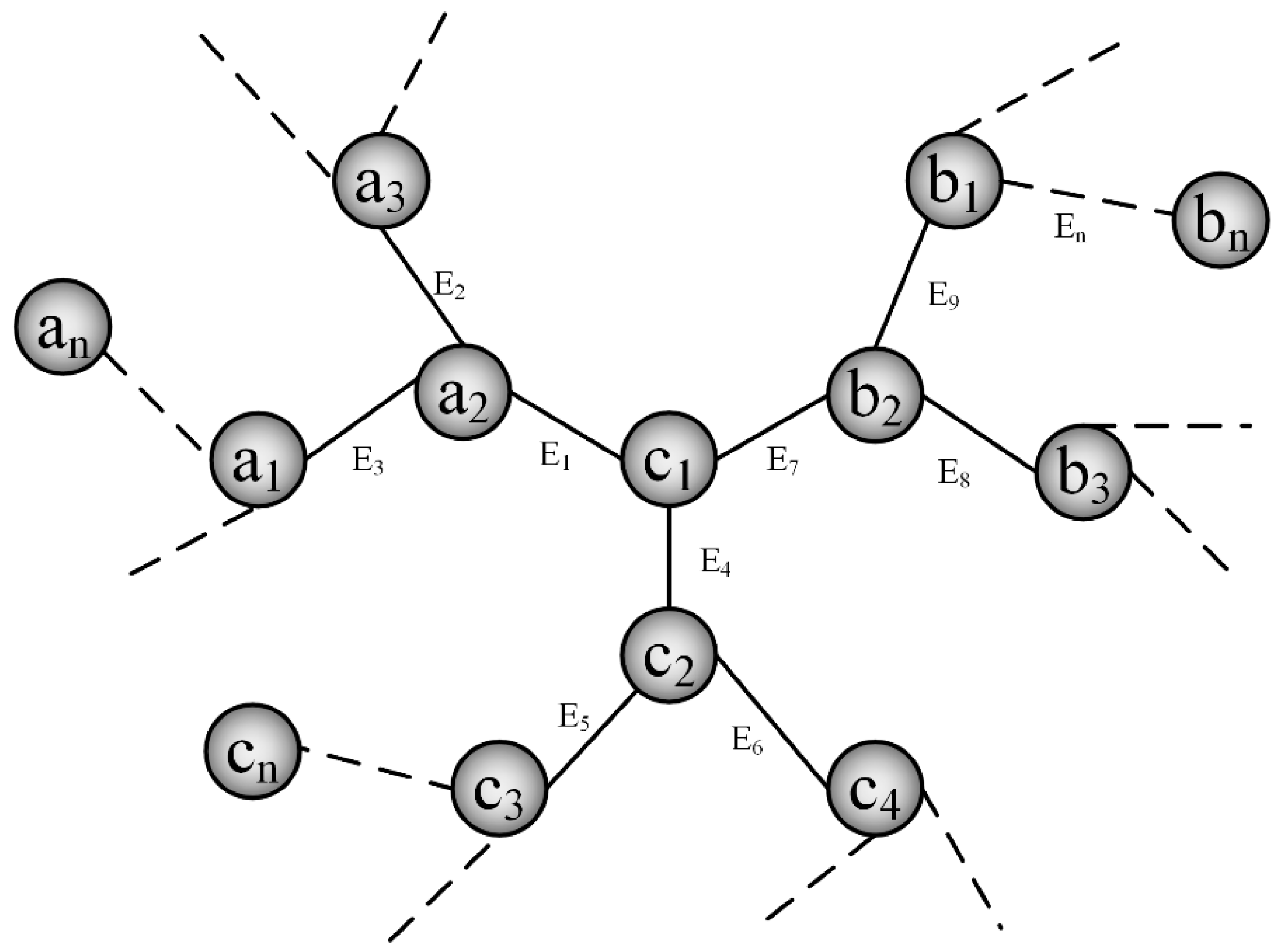
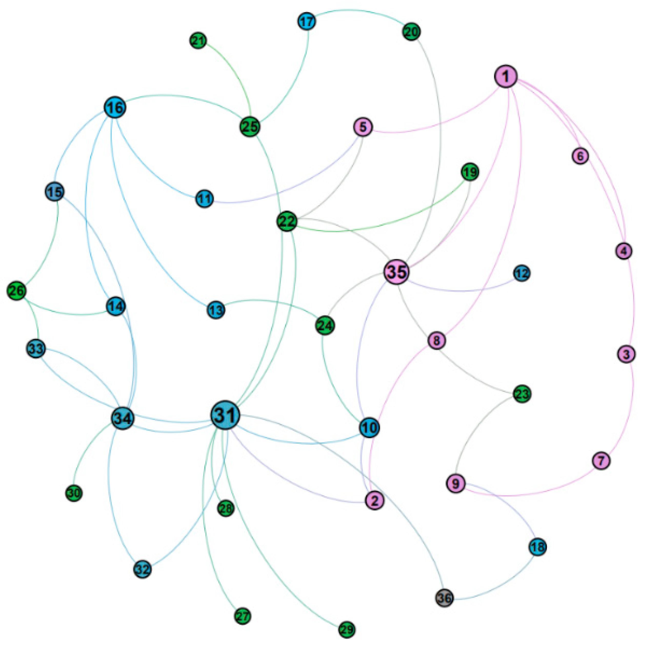
The main diagonal in the A matrix represents the edge connecting the node itself to itself, so it is 0. Figure 1 presents a network topology graph illustrating the structure of correlations among risk factors in SNF transportation.

In Figure 1, $V=\left\{V_1+V_2+V_3\right\}$ is the set of ‘vehicle, environment, human’ risk factors in the road transport network. $V_1=\left\{a_1,a_1,\cdots a_i,\cdots ,a_n,1<i<n\right\}$ is the set of risk factors related to the driver. $V_2=\left\{b_1,b_1,\cdots b_i,\cdots ,b_n,1<i<n\right\}$ is the set of risk factors of the vehicle itself. $V_3=\left\{c_1,c_1,\cdots c_i,\cdots ,c_n,1<i<n\right\}$ is the set of road environment risks. $E=\left\{E_1,E_2,\dots ,E_n\right\}$ is the correlation between the nodes of each factor in the network.

3.2. Construction of a Dynamic Risk Evolution Model for Road Transportation of SNF

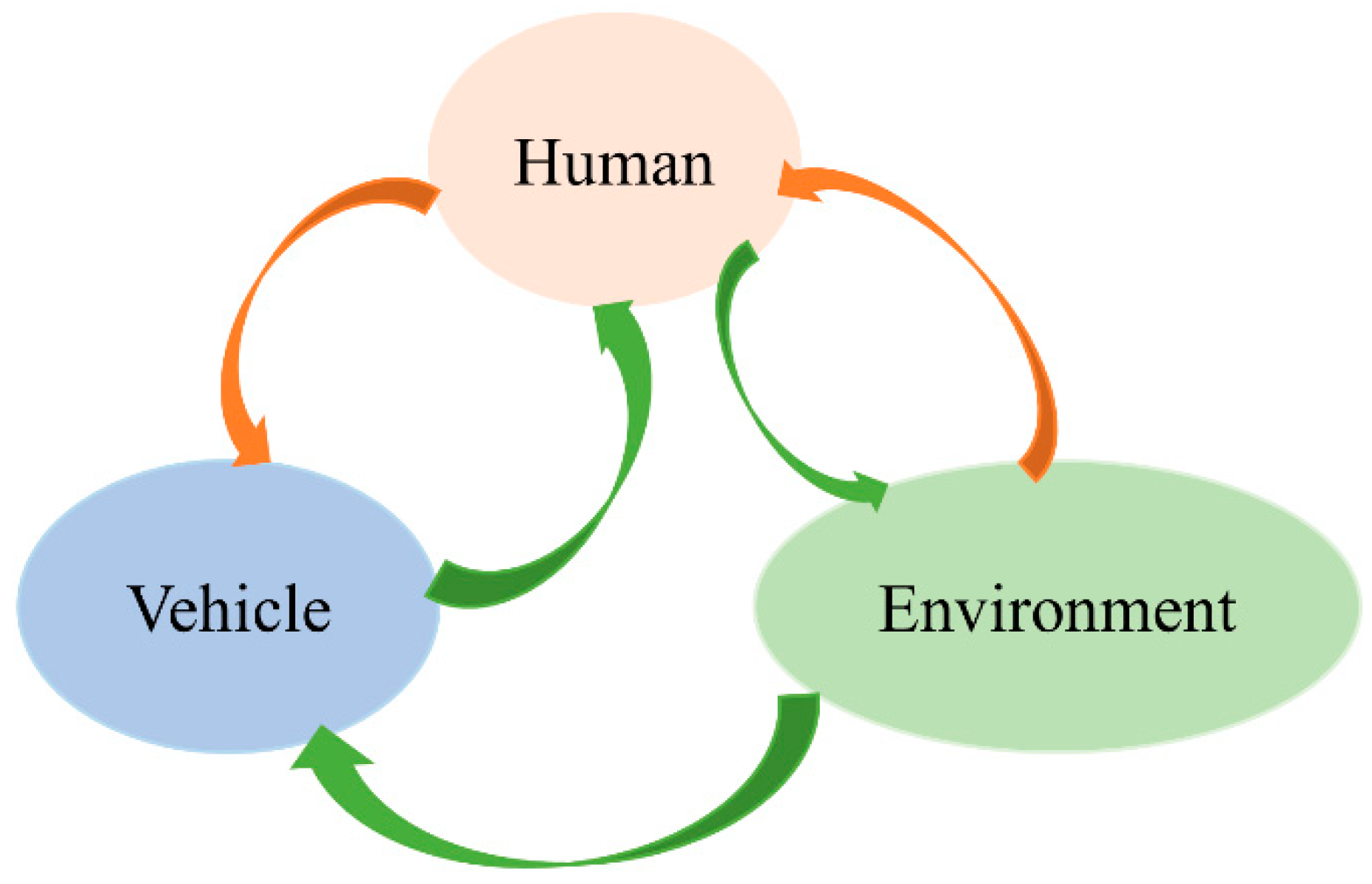
The risk factors of the SNF transportation accident are obtained based on the detailed analysis of the transportation system. This system mainly consists of three core elements: vehicle, environment and human. When an SNF transport accident occurs, the accident may result in transport cask damage or cause radioactive materials leakage. Such accidents are caused by the complex coupling and interaction of factors related to human errors, mechanical failures, and environmental conditions. In this study, the ‘vehicle–Environment–Human’ three-dimensional comprehensive risk indicator system is constructed to systematically identify and classify contributing factors in SNF transportation accidents. The risk relationship diagram between them is shown in Figure 2. This “vehicle–environment–human” structure is consistent with the man–machine–environment system safety engineering framework, in which accidents arise from the coupled behavior of human, technical, and environmental elements, rather than from isolated defects in a single component [36].

Risks stemming from the road environment exert a significant impact on the transport system, leading to corresponding changes in the driving conditions of the vehicles and in the management and driving risks of personnel [37,38]. The qualitative risk relationship diagram in Figure 2 is grounded in the well-established “human–vehicle–environment” framework in traffic safety research and in the interrelations among collision risk factors reported by Elyasi et al. [39] and Tao et al. [23]. It synthesizes findings from accident reports and expert elicitation for SNF and hazardous materials transport, capturing the main feedback loops, whereby environmental conditions affect vehicle dynamics and driver workload, vehicle malfunctions feed back into environmental and human risks, and human behavior modifies both vehicle operation and exposure to environmental hazards. The following are the relevant descriptions between the risk factors of the transportation of SNF system [39]:

(1)

Risk $f(x_i,y_i,z_i)$ in the current period is affected by the vehicle risk system $x_{i-1}$, the road environment risk system $y_{i-1}$, and the human risk system $z_{i-1}$ from the previous period.

(2)

The current risk (x_i) associated with the vehicle stems from environmental risks passed onto humans and subsequently to the vehicle in the prior period (y_i−1,z_i−1), along with the vehicle’s previous risk (ax_i−1) and the independent impact of environmental risk (y_i−1) on the vehicle.

(3)

The risk of the environment in the current period (y_i) is derived from the risk that people acted on the environment in the previous period (z_i−1) and the environmental risk level from the previous period (by_i−1).

(4)

The human’s current risk level (z_i) is influenced by their own risk in the preceding period (cz_i−1) and the risk of exposure to environmental influences from the previous period, which are transmitted from the vehicle to the person (x_i−1,y_i−1), along with the risk of direct exposure to the vehicle’s actions alone (x_i−1).

The three state variables represent aggregated risk levels in the vehicle, environment, and human subsystems. The variable $x_i$ reflects the combined effect of brake performance, steering reliability and cask integrity; $y_i$ reflects road friction, geometric design and weather and visibility; and $z_i$ reflects driver fatigue, workload and compliance with procedures. The nonlinear coupling terms describe how a change in one subsystem, such as worsening weather, feeds back into the others by reducing braking margins and increasing the driver’s cognitive load.

Based on the above descriptions, the evolutionary differential equations for the risk system of SNP transportation are shown below:

$$\left\{\begin{array}{l}{x}_i=z_{i-1}{y}_{i-1}-a{x}_{i-1}+y_{i-1}\hfill \\ y_i=z_{i-1}-b{y}_{i-1}\hfill \\ z_i=c{z}_{i-1}-x_{i-1}{y}_{i-1}+x_{i-1}\hfill \end{array}\right.$$

(3)

Equation (3) is then transformed into the following:

$$\left\{\begin{array}{l}\stackrel{·}{x}=zy-(a+1)x+y\hfill \\ \stackrel{·}{y}=z-(b+1)y\hfill \\ \stackrel{·}{z}=(c-1)z-xy+x\hfill \end{array}\right.$$

(4)

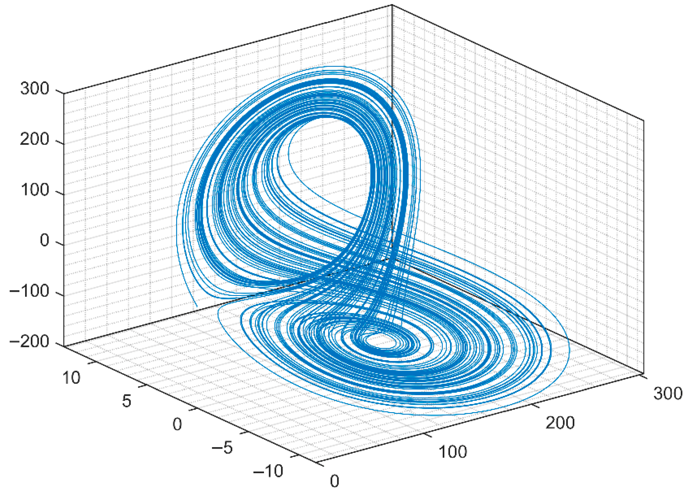
In Equation (4), when a = 3, b = 10, and c = 14, the system exhibits chaotic behavior as shown in Figure 3. Chaotic attractors have emerged, indicating that the system is unstable and in a chaotic state.

3.3. Dynamical Evolution and Chaotic Behavior Analysis

To reveal the mechanism of risk transmission within the SNF transportation system, this section investigates the system’s dynamic evolution under varying coupling parameters. Small changes in environmental conditions, in the driver’s state or in the vehicle’s condition can, through nonlinear feedback, produce disproportionately large changes in the overall risk level, particularly when operations are already close to safety margins. The nonlinear coupling terms are capable of capturing these feedback effects, and the bifurcations and positive Lyapunov exponents observed in the simulations demonstrate how such effects can drive the system from a stable to a chaotic regime.

3.3.1. Parameter Sensitivity and Bifurcation Mechanism

Models of SNF transportation risk often display complex dynamic behavior. System stability depends on the coupled interactions among the vehicle, environment, and human components. As operating conditions change, the system may evolve from a stable equilibrium to instability and eventually to chaotic behavior. In particular, the occurrence of a Hopf bifurcation marks a qualitative shift in equilibrium stability, giving rise to periodic oscillations. Accordingly, bifurcation analysis of the key risk factors a, b and c is used to identify critical thresholds associated with the onset of elevated risk.

(1)

Bifurcation analysis of parameter a

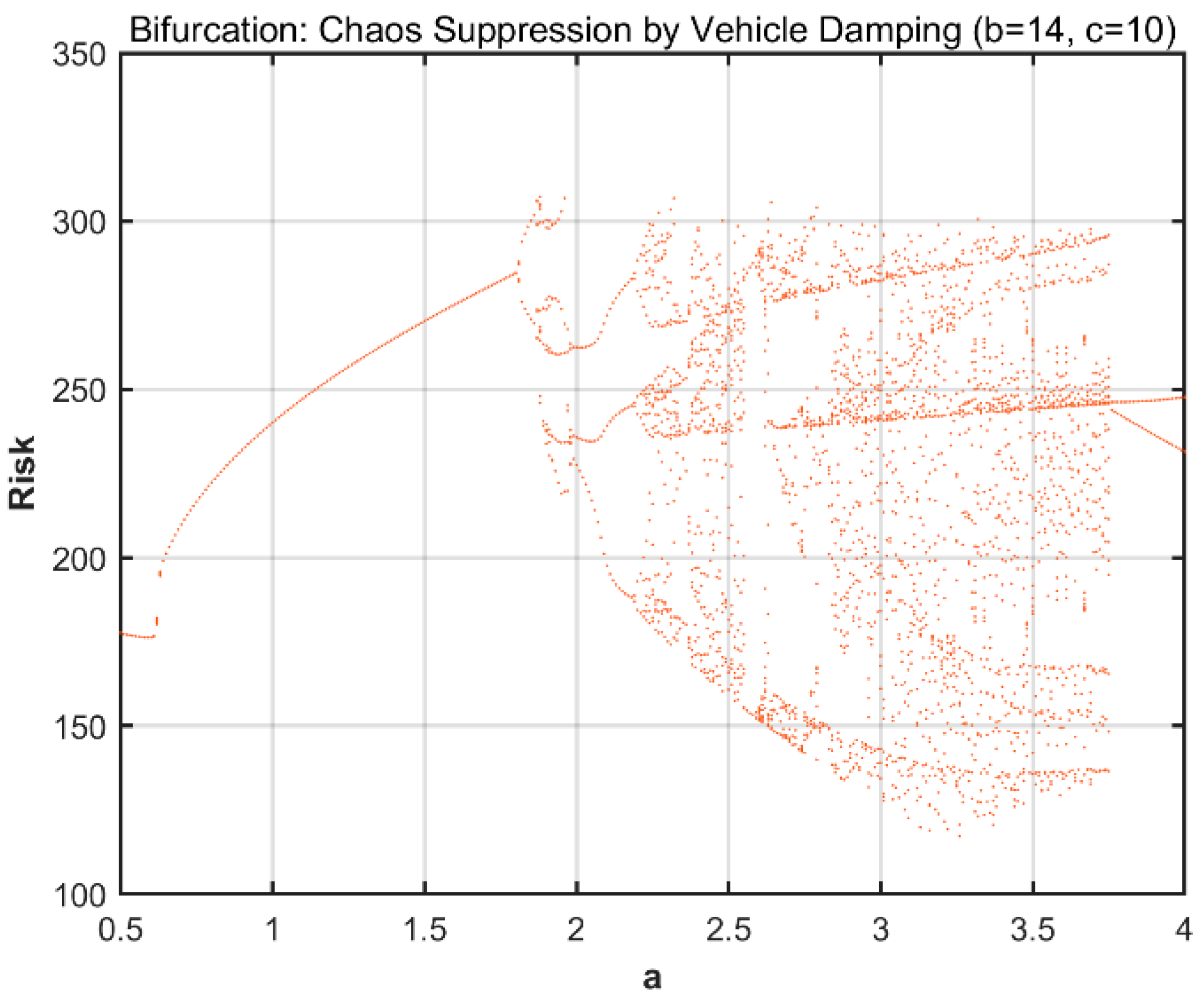
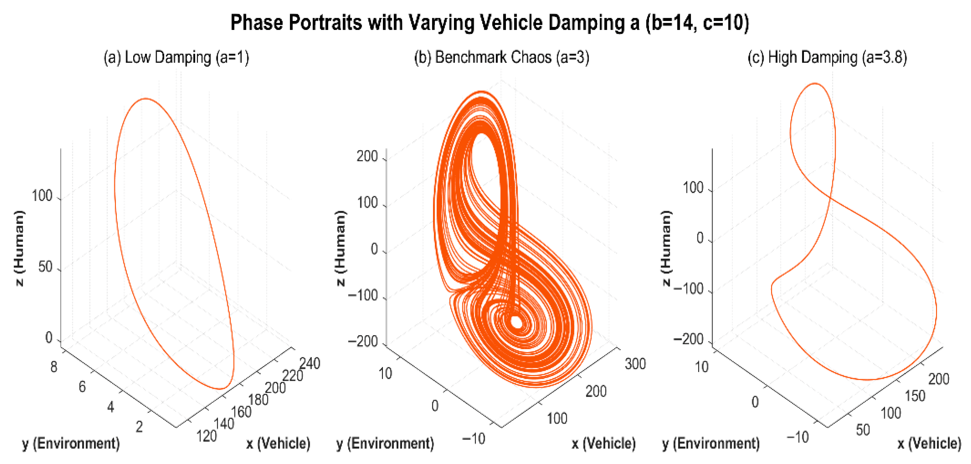
When b = 14, c = 10, and a is uncertain, simulations yielded the bifurcation diagram of $a\in [0.5,4]$, as shown in Figure 4. The corresponding phase portrait is depicted in Figure 5.

Figure 4 and Figure 5 reveal that the system evolves toward chaos via a double-period bifurcation. When the system enters an unstable chaotic state, violent disordered fluctuations pose a severe threat to the safety and stability of the SNF transport system. Therefore, regulatory strategies must be introduced at the appropriate time to suppress the system’s long-term violent oscillations and ensure transport safety.

(2)

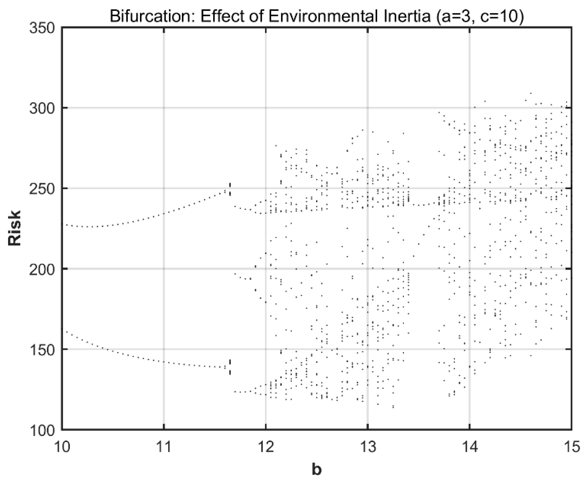
Bifurcation analysis of parameter b

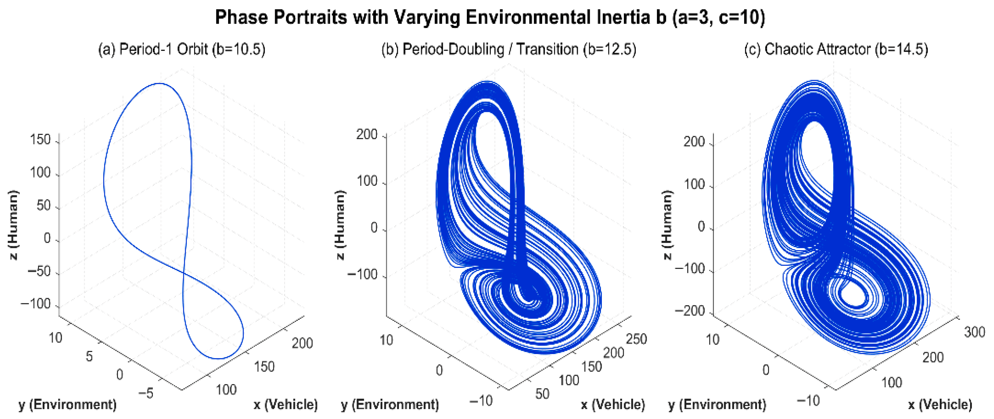
When a = 3, c = 1, and b is uncertain, simulations yielded the bifurcation diagram of $b\in [10,15]$, as shown in Figure 6. The corresponding phase portrait is depicted in Figure 7.

Figure 6 and Figure 7 clearly reveal the mechanism by which parameter b influences the dynamical behavior of the SNF transport risk system. As b gradually increases from 10 to 15, the system exhibits a classic bifurcation path from periodicity to chaos: when b lies within the interval [10, 11.6], the system operates stably on a periodic-2 orbit, with risk values oscillating rhythmically between predetermined high and low levels. As b continues to increase and surpasses the critical threshold, the system undergoes successive bifurcations, rapidly multiplying oscillation periods. Ultimately, when b > 12, the system fully evolves into a chaotic state, where risk values lose periodic regularity. This significantly increases the uncertainty and management difficulty of transport risks.

(3)

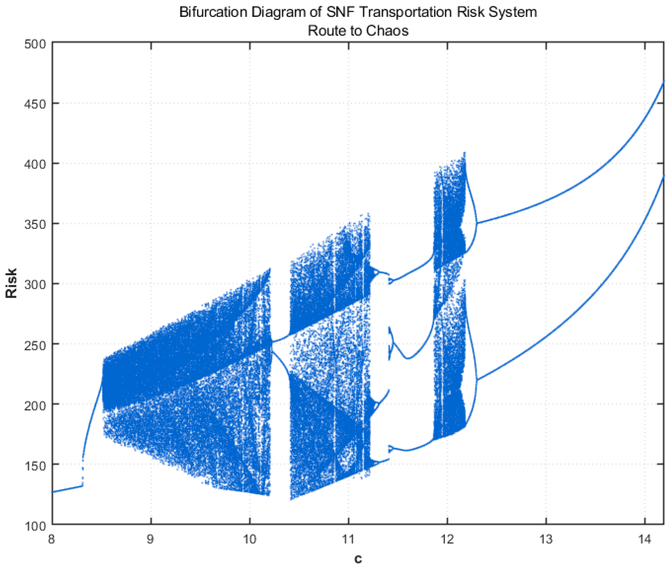
Bifurcation analysis of parameter c

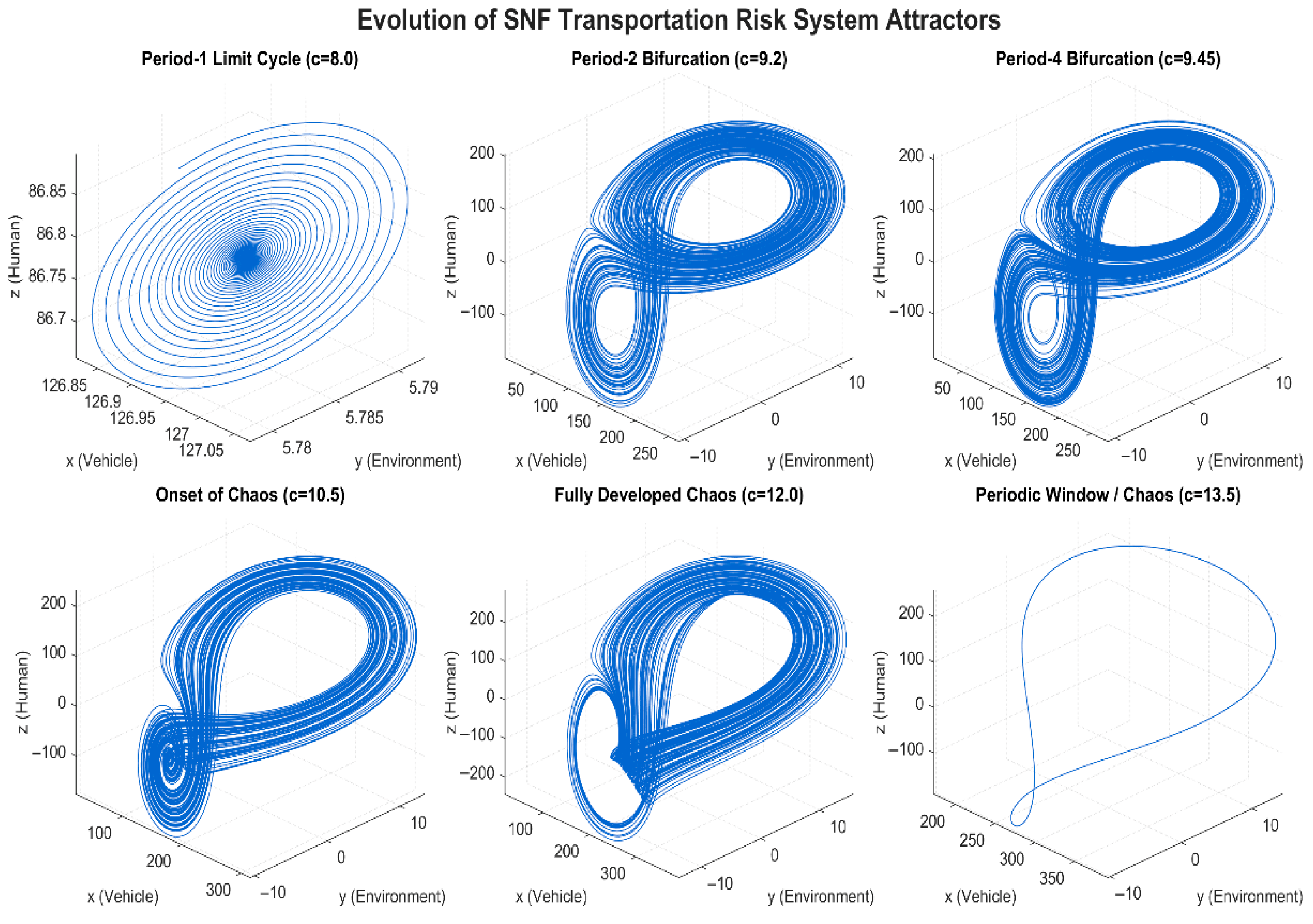
When a = 3, b = 14, and c is uncertain, simulations yielded the bifurcation diagram of $c\in [8,14]$, as shown in Figure 8. The corresponding phase portrait is depicted in Figure 9.

Figure 8 and Figure 9 reveal that parameter c exerts a significant nonlinear regulatory effect on the evolutionary trajectory of the SNF transport risk system, which exhibits a complex topological structure characterized by alternating chaotic bands and periodic windows. As c increases, the system first enters the chaotic region $c\in [8.5, 12.2]$ via bifurcation. Within this interval, risk evolution exhibits high sensitivity to initial conditions and ergodicity, yet simultaneously embeds multiple distinct stability windows at 10.3 and 11.3, revealing paroxysmal characteristics in the risk oscillation process.

3.3.2. Chaotic Attractor and Quantitative Verification

To definitively confirm the existence of chaos, we focus on the representative parameter set [a, b, c] = [3, 10, 14], located within the chaotic region identified above. In this context, the Lyapunov exponent serves as a critical indicator for quantitatively verifying the system’s dynamic behavior. Theoretically, this exponent describes the rate of separation of infinitesimal trajectories: a negative exponent implies that the system stabilizes regardless of the initial state; a zero exponent indicates a critically stable state; A positive Lyapunov exponent indicates that adjacent trajectories diverge exponentially, signifying the presence of chaotic behavior in the system. Compared to simple phase space plots, the Lyapunov exponent provides a clearer observation of the system’s sensitivity to initial conditions and its dissipative properties [40]. If a system is in a chaotic state, it will inevitably have a Lyapunov exponent greater than zero. Therefore, the value of the Lyapunov exponent acts as a criterion in determining whether the system is in chaos. As the dynamical system evolves, the point’s trajectory expands or contracts in all directions within the phase space. The rate of increase of $f\left(x_i\right)$ for the i-th Lyapunov index running trajectory at time i is defined as follows:

$$\lambda \left(x_0\right)=\underset{n\to \infty }{\lim }{\displaystyle \frac{1}{n}}\sum _{i=0}^{n-1}\ln \left|F^{\prime }\left(x_i\right)\right|$$

(5)

$\lambda \left(x_0\right)$ denotes the n-dimensional Lyapunov exponent when the base approaches zero. Sorting these n Lyapunov exponents from largest to smallest gives a spectrum of Lyapunov exponents shown below:

$${\lambda }_1\ge {\lambda }_2\ge \cdots \ge {\lambda }_n$$

(6)

Through Equation (4), the equation of the constant state of the system is assumed to be expressed as follows:

$$\begin{array}{l}z\mathrm{y}-(a+1)x+y=0\hfill \\ z-(b+1)y=0\hfill \\ (c-1)z-xy+x=0\hfill \end{array}$$

(7)

The above equation is linearized to obtain the corresponding Jacobian matrix, expressed as follows:

$$\left[\begin{array}{ccc}-a-1& z+1& y\\ 0& -b-1& 1\\ 1-y& -x& c-1\end{array}\right]$$

(8)

The eigenvalue determinant is given as follows:

$$\left|\begin{array}{ccc}-a-1-\lambda & z+1& y\\ 0& -b-1-\lambda & 1\\ 1-y& -x& c-1-\lambda \end{array}\right|=0$$

(9)

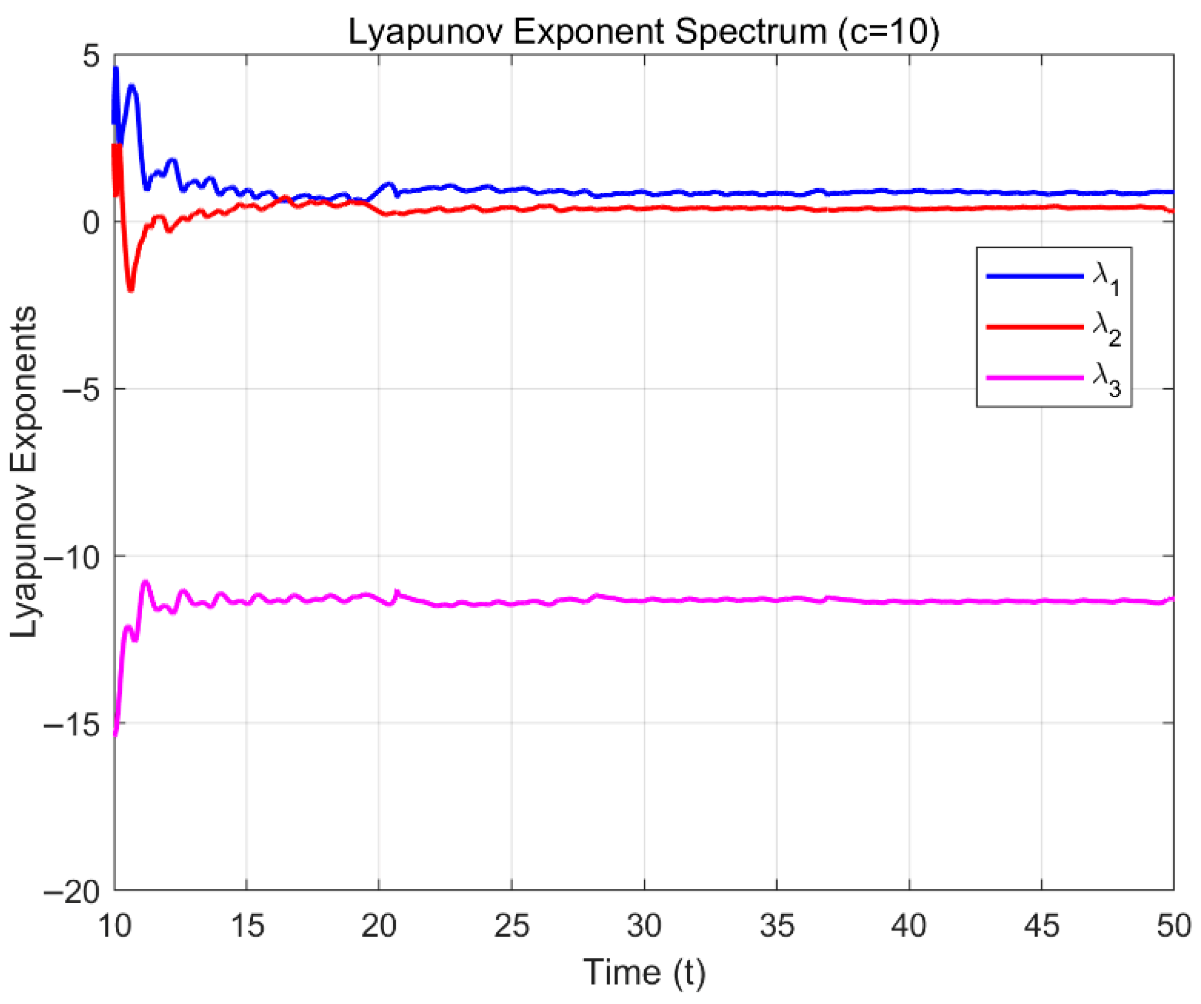
Substituting (x,y,z) = [0,0,0] into the Jacobian matrix yields the eigenvalue A, indicating that this equilibrium point is unstable in the SNF transport risk system. The existence of an unstable equilibrium reflects inherent system instability, which provides the conditions for chaotic behavior that can undermine transport safety. For the parameter values a = 3, b = 10, and c = 14, the corresponding Lyapunov exponent spectrum is presented in Figure 10.

As shown in Figure 10, the system exhibits a distinct positive maximum Lyapunov exponent, indicating that risk evolution is sensitive to initial conditions. Furthermore, the sum of the Lyapunov exponents converges to a negative value, signifying that the system is dissipative. This implies that while local trajectories diverge chaotically, the global phase space volume contracts, ultimately confining the risk state within a bounded singular attractor.

3.4. Design of Chaotic Controllers

From a control perspective, we use Lyapunov-based synchronization because it offers a strict and transparent way to ensure that the difference between the driver and responder systems steadily decreases to zero, even when their interactions are nonlinear.

Chaotic synchronization control is implemented using a driver–responder system method. In this method, an active controller is applied to the responder system to guide its state toward that of the driver system over time. As a result, the difference between the two system states becomes stable and gradually diminishes to zero. This process effectively suppresses the system’s sensitivity to initial conditions by eliminating deviations between system states through control measures, the system recovers and maintains stability on a synchronous manifold. In this method, the driver system represents the system’s natural dynamic behavior in the absence of control and provides the reference trajectory for synchronization. The responder system represents the actual operating system, which is subject to safety constraints and external control. The controller embodies the specific control strategy, including active safety measures such as real-time route adjustment or emergency braking.

The design of the driving system, response system, and controller is expressed by the following equations:

Drive system:

$$\left\{\begin{array}{l}\stackrel{·}{x_1}=z_1{y}_1-(a+1)x_1+y_1\hfill \\ \stackrel{·}{y_1}=z_1-(b+1)y_1\hfill \\ \stackrel{·}{z_1}=(c-1)z_1-x_1{y}_1+x_1\hfill \end{array}\right.$$

(10)

Response system:

$$\left\{\begin{array}{l}\stackrel{·}{x_2}=z_2{y}_2-(a+1)x_2+y_2-u_1\hfill \\ \stackrel{·}{y_2}=z_2-(b+1)y_2-u_2\hfill \\ \stackrel{·}{z_2}=(c-1)z_2-x_2{y}_2+x_2-u_3\hfill \end{array}\right.$$

(11)

Here, $u_1$, $u_2$, $u_3$ are the controllers to be designed. In practice, the control inputs k_i correspond to adjustable safety actions in the vehicle, environmental, and human domains, such as applying dynamic speed limits, diverting traffic to safer routes, or issuing real-time warnings about fatigue and poor visibility. The gain coefficients ki determine how strongly each of these actions is applied in response to the current risk level.

Setting the error system $e(t)=(11)-(10)$, the dynamical system for the error equation is obtained as follows:

$$\left\{\begin{array}{l}\stackrel{·}{e_1}=y_2{e}_3+z_1{e}_2-e_1(a+1)+e_2-u_1\\ \stackrel{·}{e_2}=e_3-(b+1)e_2-u_2\\ \stackrel{·}{e_3}=(c-1)e_3-x_1{e}_2-y_2{e}_1+e_1-u_3\end{array}\right.$$

(12)

where $e_1=x_2-x_1,e_2=y_2-y_1,e_3=z_2-z_1$ is the state error in Equations (10) and (11).

The above description transforms the synchronization problem of the response system (11) and the drive system (10) into an asymptotic stability problem at the origin in the error dynamics system, and by adding the control gains $f_i$ (i = 1, 2, 3) > 0, the expression for the controller is determined to be:

$$\left\{\begin{array}{l}{u}_1=y_2{e}_3+z_2{e}_2-e_1(a+1)+e_2+k_1{e}_1\\ u_2=e_3-(b+1)e_2+k_2{e}_2\\ u_3=(c-1)e_3-x_1{e}_2-y_2{e}_1+e_1+k_3{e}_3\end{array}\right.$$

(13)

where k_i (i = 1, 2, 3) denotes the increment control coefficients.

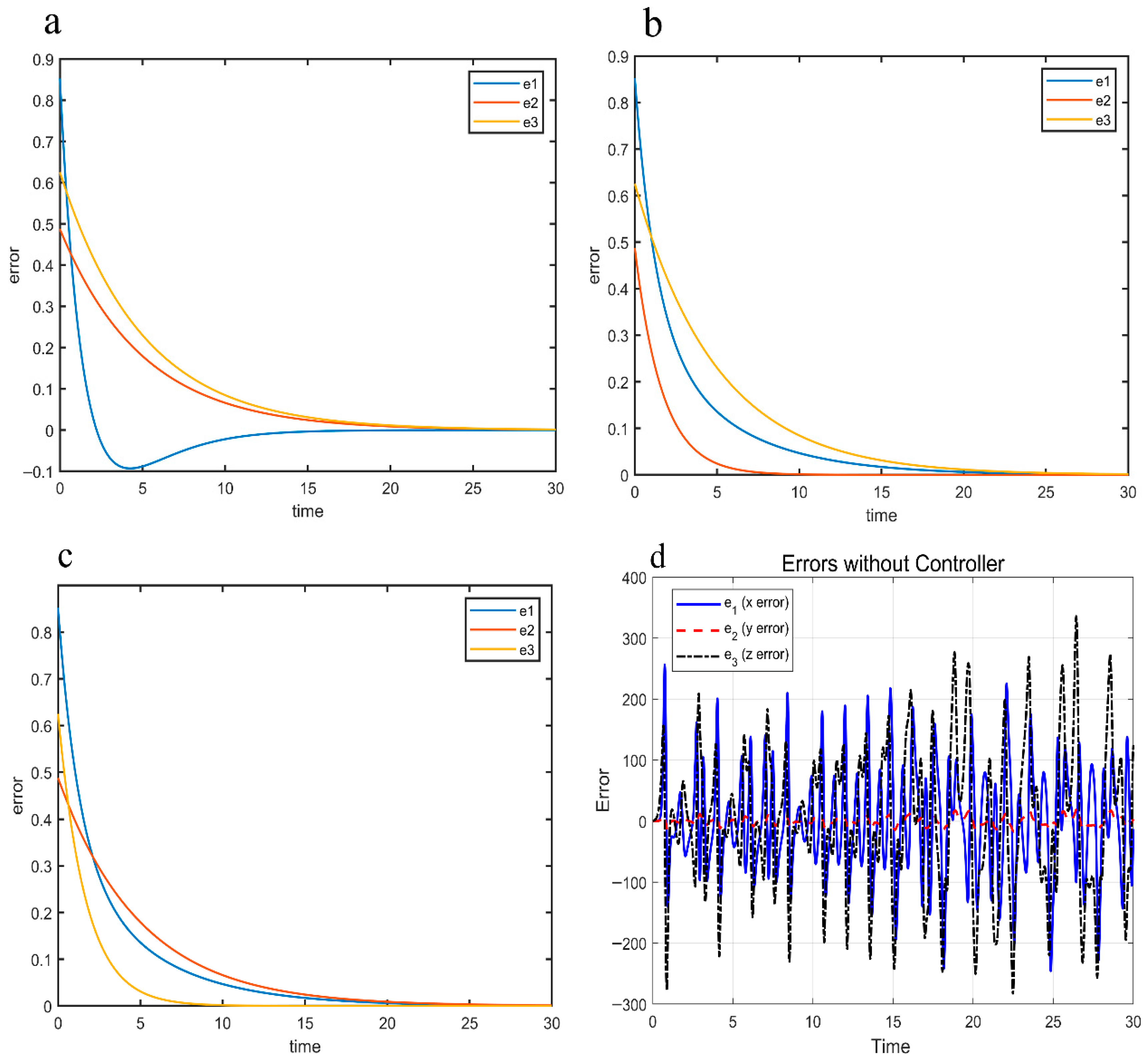
Equations (10) and (11) are given arbitrary initial values under the action of the controller (13), and the error system risk slowly stabilizes with the evolution of time. The expressions are as follows:

$$\underset{t\to 0}{\lim }\left|e_i(t)\right|=0,i=1, 2, 3$$

(14)

The design of the above controller is demonstrated as follows:

First, construct a Lyapunov function:

$$V(t)={\displaystyle \frac{1}{2}}(e_1^2+e_2^2+e_3^2)$$

(15)

Next, the derivation of Equation (15) gives the following result:

$$\stackrel{·}{V}=-k_1{e}_1^2-k_2{e}_2^2-k_3{e}_3^2$$

(16)

when $k_i>0$, it can be shown that $\stackrel{·}{V}<0$. The risk error system (12) equation is asymptotically stabilized under the controller Equation (13) and converges to the origin. The risk system gradually approaches chaotic synchronization, and the risk transport system reaches a steady state.

4. Numerical Simulation

4.1. Risk Factor Identification

In many countries, including those in Europe, rail is commonly used for transporting spent fuel because of its lower degrees of freedom and strict operational rules. In China, SNF is also transported using multimodal road–rail systems. The present study focuses on the road segment which connects nuclear power plants to rail freight stations and final destinations. This segment remains a critical source of operational risk even when rail is used for the long-distance portion of the route. To evaluate the applicability of the proposed model, this study considers a representative scenario in which spent fuel assemblies from a pressurized water reactor are transported from the Daya Bay Nuclear Power Base to the spent fuel reprocessing facility of China National Nuclear Corporation’s 404 Plant. The Daya Bay Nuclear Power Base is one of the world’s largest pressurized water reactor facilities, with a total installed capacity of 6.12 GW. Over nearly three decades of operation, it has generated approximately 1 trillion kWh of electricity, primarily serving the Guangdong–Hong Kong–Macao Greater Bay Area. Approximately 70–80% of this electricity is supplied to Hong Kong, and the facility produces about 40–50 tons of spent fuel each year. Spent fuel is transported to the CNNC 404 Plant using a road–rail intermodal system, with a total transport distance of approximately 4120 km. The road transport segment, which connects the plant to the rail freight station, covers roughly 80 km. For the road transport segment, the relevant “vehicle–environment–personnel” system risk factors are shown in

Table 1. Risk factors for road transport of SNF.

Risk Categories		Node	Risk Factors
Categories of Human Management Risks		1	Fatigued driving
		2	Speeding
		3	Careless operation
		4	Illegal operation
		5	Operation error
		6	Poor mental state
		7	Inadequate knowledge and experience
		8	Other violations
		9	Mismanagement
		35	Unsafe distance between cars
Categories of Vehicle Risk Management Factors		10	Vehicle brake failure
		11	Steering wheel malfunction
		12	Flat tire
		13	Engine stalled
		14	Tire fire
		15	Fuel tank fire
		16	Other vehicle braking failures
		17	Monitoring equipment failure
		18	Failure of spent fuel transportation containers
		31	Vehicle collisions
		32	Squeeze
		33	catch fire
		34	blast
Environmental Risk Management	Climate Risk Factors	24	Severe weather
		25	Geological hazards
	Road Risk Factors	19	Road slippery
		20	Poor lighting conditions
		21	Uneven road surface
		22	Poor line design (steep slopes, sharp turns, long descents)
		23	Lack of safety warning signs
		26	Malicious social environment
		27	Nearby traffic accidents
		28	Pedestrians crossing the road
		29	Animals crossing the road
		30	Major hazards in the vicinity
		36	Nearby vehicles

.

Table 1 summarizes the risk factors identified through a systematic statistical analysis of traffic accident data [41,42,43,44]. They cover multiple dimensions, including vehicle-related conditions, environmental factors, and human behavior, such as driver actions, vehicle status, road quality, and weather and lighting conditions. The set of factors for human management risk in Table 1 is $T_1=\left\{1,2,3,4,5,6,7,8,9,35\right\}$. The set of vehicle risk management factors is $T_2=\left\{10,11,12,13,14,15,16,17,18,31,32,33,34\right\}$. The collection of factors for road environmental risk management is $T_3=\left\{19,20,21,22,23,24,25,26,27,28,29,30,36\right\}$. The numbers assigned to each factor are for reference and citation purposes only and do not indicate any order of priority or causal sequence.

4.2. Calculate the Importance of Risk Factors

The higher the importance of a triggered risk factor, the more pronounced the cascade of risks, escalating the likelihood of system vulnerability and increasing the risk of traffic accidents. Thus, based on the correlation between the risk factors of SNF, a risk-related factor association diagram is established, as shown in Figure 11, where each risk factor represents a node V and the edge E is the risk correlation between the nodes, indicating that factor i is related to factor j. For example, in the context of SNF transportation: Environmental–Vehicle Coupling: “Severe weather” V₂₄ leads to “ road slippery” V₁₉, which significantly degrades the braking efficiency of the heavy-duty SNF truck, effectively triggering “Vehicle brake failure” V₁₀. Human–System Coupling: “Fatigued driving”V₁ directly increases the probability of “Operation error” V₅, which serves as a direct precursor to “Vehicle collisions” V₃₁.

In Figure 11, the purple nodes denote human-related risk factors, the blue nodes represent vehicle-related risks, and the green nodes correspond to environmental risks. The network structure shows that these risk factors are interconnected and influence one another.

The correlation value of significance serves as a metric for the importance of each risk factor within the system. To further quantify and identify high-influence diffusion nodes associated with these risk factors, this study employs an improved K-shell algorithm integrated with node information entropy (IKS) [45]. This algorithm overcomes the limitation of the traditional K-shell method in neglecting node topological position information, enabling it to accurately identify critical diffusion nodes in both high and low shell layers while enhancing the precision of diffusion risk assessment. The influence capacity of a network node is determined by introducing information entropy. The calculation steps of the method are as follows:

Step 1. Let the degree of the node $v_i$ be $k_i$, the node importance be $I_i$, and the node information entropy be $e_i$. The expressions are as follows:

$$I_i={\displaystyle \frac{k_i}{{\displaystyle \sum _{j=1}^N}{k}_j}}$$

(17)

$$e_i=-\sum _{j\in \mathsf{\Gamma }(i)}{I}_j\cdot \ln I_j$$

(18)

Step 2. The network is layered using a typical K-shell algorithm to obtain the K-value of each node.

Step 3 calculates the information entropy of each node and numbers in increasing order.

Step 4. Select the node in the next layer of the shell with the highest entropy of node information until the node is selected in the K-shell and the first iteration is complete.

Step 5. Repeat Step 4 to select the remaining nodes until all nodes are selected, ignoring the shells of all nodes selected. Nodes are selected randomly in a given shell layer when the node information entropy values are equal.

Based on the above K-shell method, the importance of each risk factor in the transportation of SNF by road are computed and detailed in

Table 2. The importance of each risk factor.

Categories	Node	Value of Importance of Risk Factors	Categories	Node	Value of Importance of Risk Factors	Categories	Node	Value of Importance of Risk Factors
Human	1	0.5409	Vehicle	10	0.6395	Environment	19	0.3226
	2	0.4389		11	0.2482		20	0.2733
	3	0.2406		12	0.1973		21	0.1253
	4	0.1646		13	0.2482		22	0.6132
	5	0.3659		14	0.4128		23	0.2996
	6	0.1646		15	0.4128		24	0.3986
	7	0.1783		16	0.4818		25	0.5042
	8	0.2669		17	0.2013		26	0.3068
	9	0.2280		18	0.1783		27	0.2376
	35	0.7901		31	1.000		28	0.2376
				32	0.4022		29	0.2376
				33	0.5045		30	0.1646
							36	0.3136

.

Table 2 shows that, for the vehicle, environment and human dimensions, the minimum importance values are 0.1783 for node 18, failure of spent fuel transportation containers, 0.1253 for node 21, uneven road surface, and 0.1646 for node 6, poor mental state. The corresponding maximum values are 1.000 for node 31, vehicle collisions, 0.6132 for node 22, poor line design with steep slopes, sharp turns and long descents, and 0.7901 for node 35, unsafe distance between vehicles. These normalized importance scores, all lying between 0 and 1, indicate the relative influence of each factor on risk propagation within the network.

4.3. Verification of the Controller

In order to validate the effectiveness of the proposed chaotic synchronization controller, we simulate the process of guiding the system from a high-risk chaotic state to a low-risk stable state. The drive system is initialized using the minimum importance values of the risk factors derived from the K-shell analysis (Table 2). These correspond to Node 18 (Failure of spent fuel transportation containers, 0.1783) for the vehicle dimension, Node 21 (Uneven road surface, 0.1253) for the environmental dimension, and Node 4 (Illegal operation, 0.1646) for the human dimension. Consequently, the initial condition of the drive system is set as $(x_1,y_1,z_1)=(0.1782,0.1253,0.1645)$. Conversely, the response system (representing the initial uncontrolled state) is initialized using the maximum importance values, simulating a worst-case scenario. These correspond to Node 31 (Vehicle collisions, 1.000), Node 22 (Poor line design, 0.6132), and Node 35 (Safe distance between cars, 0.7901), respectively. Thus, the initial condition of the response system is set as $(x_2,y_2,z_2)=(1,0.613,0.79)$. Based on these initial conditions, three distinct control scenarios are designed to evaluate system convergence, as outlined in

Table 3. Options for systematic control of risks in the transportation of SNF.

	K1	K2	K3
Programs control of the main vehicle risks (Scenario a)	0.6	0.2	0.2
Programs for the control of the main environment risks (Scenario b)	0.2	0.6	0.2
Programs for the control of the main human risks (Scenario c)	0.2	0.2	0.6

.

The increment control coefficients k_i (i = 1, 2, 3) in Table 3 were used for the control ratios in ‘vehicle–environment–human’ to measure the degree of control in each risk dimension. According to Equations (10)–(13), the initial value of Equation (10) is set as the minimum importance value of each dimension of the transportation risk system, which is 0.1782, 0.1253, and 0.1645, respectively; meanwhile, the initial value of Equation (11) is set as the maximum importance value of each dimension of the transportation risk system, which is 1, 0.613, and 0.79, respectively. On the basis of the three scenarios in Table 3, the calculated risk control results of the transportation risk system are shown in Figure 12.

As shown in Figure 12, introducing the transportation risk controller gradually stabilizes the error dynamics by synchronizing the states of the driver and responder systems, thereby achieving effective control of the chaotic risk process. Using the proposed synchronization control method, we examine how different categories of risk affect system stability under three targeted strategies listed in Table 3: a vehicle-focused strategy, Scenario a with gain K₁ = 0.6; an environment-focused strategy, Scenario b with gain K₂ = 0.6; and a human-focused strategy, Scenario c with gain K₃ = 0.6. The simulation results show that both the environment-focused strategy and the human-focused strategy lead to faster convergence of the system than the vehicle-focused strategy. In particular, assigning a gain of 0.6 to either environmental control or human-related management, which corresponds to allocating about 60 percent of the control effort to the environment or to personnel, effectively suppresses risk divergence and drives the system rapidly toward a stable state. By contrast, when no control input is applied, the system error, as illustrated in Figure 12d, remains in a persistent chaotic oscillatory state and does not converge, indicating that the uncontrolled transport risk system is inherently unstable. Overall, these results suggest that prioritizing environmental management or human-factor management, rather than focusing mainly on the vehicle, is more effective for achieving timely stabilization of transport risk. Although our study evaluates these control rules through numerical simulations, they can be integrated into real-time decision support systems that translate the abstract control signals into concrete operational measures, including automated dispatch recommendations, adjustments to driver assistance systems, or temporary road closures. These results provide a clear theoretical basis for SNF transportation management, indicating that real-time environmental monitoring and response mechanisms are the most effective means of suppressing instability when resources are limited.

5. Conclusions

This paper constructs a dynamic evolution model of the SNF transportation risk system based on chaos theory, revealing the nonlinear coupling mechanism between risk factors and the system’s chaotic characteristics. The main conclusions drawn from this study are as follows:

(1)

Chaotic Modeling: A chaotic dynamics model for the SNF highway transportation system is developed based on the “Human–Vehicle–Environment” coupling relationship. By designing a chaotic synchronization controller, the transition of the transport risk system from a divergent chaotic state to a stable synchronized state is successfully achieved, providing a mathematical method for dynamic risk evolution analysis.

(2)

Risk Identification: Based on graph theory, the topological relationship of SNF transport risk factors is established. An improved K-shell decomposition algorithm is utilized to calculate the global influence of risk nodes, effectively identifying critical risk factors. These relative importance values serve as the quantitative basis for determining the initial parameters of the drive and response systems.

(3)

Control Strategy Evaluation: The effects of different risk control dimensions on system stability are evaluated using a chaotic synchronization method. Specifically, three targeted control strategies listed in Table 3 are examined: a vehicle/cask-focused strategy (Scenario a), an environment-focused strategy (Scenario b), and a human-focused strategy (Scenario c). Numerical simulations demonstrate that the environment-focused strategy (Scenario b) performs best, reducing system errors to zero within approximately 12 time steps. By comparison, the human-focused strategy (Scenario c) and the vehicle/cask-focused strategy (Scenario a) require about 20 and 30 time steps, respectively, to achieve synchronization. As a result, prioritizing environmental risk mitigation improves convergence efficiency by approximately 40% and 60% relative to the other two strategies. These findings provide a clear theoretical basis for SNF transportation management, indicating that real-time environmental monitoring and response mechanisms are the most effective means of controlling system instability under limited resources.

To ensure the safety and robustness of radioactive material transport, operators must establish a multi-tiered, proactive risk prevention and control system. The core of this system lies in dynamically optimizing and adjusting transport routes based on real-time meteorological data and road network monitoring information, prioritizing avoidance of extreme weather zones and densely populated areas to systematically reduce potential collective dose risks. Given the heavy weight and high inertia of high-level radioactive waste transport containers, specialized structural load-bearing capacity and slope safety assessments must be conducted for critical infrastructure such as bridges and tunnels along the planned route. This prevents instability or failure caused by vehicle–environment dynamic coupling. Additionally, chaotic synchronous control mechanisms should be deeply integrated into the transport monitoring platform. By continuously collecting and analyzing critical environmental parameters like road friction coefficients and visibility, the system enables proactive early warnings. It actively alerts drivers to risks while simultaneously triggering vehicle stability control systems, establishing a coordinated ‘machine–environment–human’ proactive defense model rather than relying on reactive post-event responses. Although this study focuses on SNF, the proposed ‘network-chaos’ framework possesses general applicability. It can be extended to other hazardous materials, such as hydrogen or LNG transportation, by recalibrating the risk nodes and adjusting the coupling parameters. The present study is mainly methodological and simulation-based, and does not yet include a full benchmark against PSA, Bayesian networks or machine learning models. In future work, we will calibrate the model with historical SNF or hazardous-materials accident data and compare it with data-driven and traditional static methods in terms of predictive accuracy, computational cost and interpretability.