Efficient and Spatially Aware 3D Gaussian Splatting for Compact Large-Scale Scene Reconstruction

Abstract

While 3D Gaussian Splatting (3DGS) has significantly advanced large-scale 3D reconstruction and novel view synthesis, it still suffers from high memory consumption and slow training speed. To address these issues without compromising reconstruction quality, we propose a novel 3DGS-based framework tailored for large-scale scenes. Specifically, we introduce a visibility-aware camera selection strategy within a divide-and-conquer training approach to dynamically adjust the number of input views for each sub-region. During training, a spatially aware densification strategy is employed to improve the reconstruction of distant objects, complemented by depth regularization to refine geometric details. Moreover, we apply an enhanced Gaussian pruning method to re-evaluate the importance of each Gaussian, prune redundant Gaussians with low contributions, and improve efficiency while reducing memory usage. Experiments on multiple large-scale scene datasets demonstrate that our approach achieves superior performance in both quality and efficiency. With its robustness and scalability, our method shows great potential for real-world applications such as autonomous driving, digital twins, urban mapping, and virtual reality content creation.

1. Introduction

Reconstructing large-scale 3D scenes, which typically span over 1.5 km², with high fidelity is a fundamental challenge in computer vision and graphics, with broad applications in fields such as autonomous driving [1,2,3,4], virtual reality [5], and aerial surveying [6]. Many methods [7,8,9,10] have attempted to extend Neural Radiance Fields (NeRF) [11] to large-scale scene reconstruction, but they often suffer from poor quality and slow rendering.

Recent advancements in 3D Gaussian Splatting [12] have demonstrated remarkable performance in photorealistic novel view synthesis and high-quality 3D reconstruction. However, given that 3DGS often requires millions or even tens of millions of Gaussians to depict scene details during training, especially for large-scale scenes, many methods [13,14,15,16] use a divide-and-conquer strategy to divide the scene into multiple blocks and deploy them on multiple GPUs for training to alleviate the problems of insufficient memory and excessive time requirements. Nevertheless, parallel training introduces a new problem, namely how to balance the training time of multiple blocks and the consistency between block boundaries. Additionally, large-scale scenes often contain diverse objects with complex geometric structures that require a large number of Gaussians to describe, such as vegetation, high-rise buildings, and roads. The adaptive densification strategy proposed by vanilla 3DGS can alleviate the above problem to a certain extent, but it is overly dependent on the initial point cloud quality and is prone to blurring and artifacts in areas where the point cloud is sparse. At the same time, Gaussian pruning based only on opacity is insufficient to accurately assess the contribution of each Gaussian to the reconstruction quality, often resulting in the erroneous deletion of important Gaussians while leaving behind persistent floaters—an issue that is particularly pronounced in large scenes.

To address aforementioned issues, we propose a brand new framework tailored for large-scale scene reconstruction. Following the previous methods [7,13,15], we split the scene into multiple blocks to train in parallel using multiple GPUs. We adopted a visibility-based camera selection to evaluate the importance of all cameras for each block, and introduced an adaptive parameter based on point cloud density to control the number of registered cameras, which can both eliminate artifacts caused by insufficient training and balance the VRAM burden of each block. To improve rendering fidelity, we proposed spatial-aware density control to mitigate the lack of densification of distant objects caused by the sparse initial point cloud and prevent the growth of floating objects near the lens. In view of the massive computing resource requirements faced by large-scale scene reconstruction, we re-evaluated the importance of each Gaussian and prune redundant Gaussians with low contributions while ensuring rendering quality. Additionally, we introduced a depth regularization loss based on Pearson correlation, which emphasizes relative depth consistency over absolute accuracy, making it well-suited for handling the scale ambiguity of monocular depth priors.

Our contributions are summarized as follows:

• We propose a novel large-scale scene reconstruction method based on 3DGS, which can achieve better rendering quality than state-of-the-art methods.
• We present a balanced data partitioning strategy to evenly manage memory consumption and training time across blocks, and modify the densification scheme to enhance the details of faraway objects in the scene.
• We optimize the Gaussian pruning step and introduce the depth regularization to improve the geometric details of the scene.

2. Related Work

2.1. Novel View Synthesis

Novel view synthesis (NVS) aims to synthesize a target image with an arbitrary target camera pose from given source images and their camera poses. As one of the most influential works in this field, Neural Radiance Fields (NeRF) [11] implicitly models various scenes through multi-layer perceptions (MLPs). Despite its remarkable ability to generate photorealistic novel views, NeRF faces significant challenges in terms of scalability and training efficiency, particularly when applied to large-scale or complex outdoor environments. These limitations have motivated a wide range of extensions aimed at improving its representational power, accelerating its rendering speed, and enhancing its adaptability to diverse and unconstrained real-world scenarios. Plenoxels [17] represents a scene as a sparse 3D grid with spherical harmonics, optimized from calibrated images using gradient methods and regularization, without neural components. Various strategies [18,19,20,21] have been proposed to enhance rendering efficiency and minimize memory consumption. More recently, 3DGS [12] achieved impressive NVS performance, excelling in both rendering quality and speed, by leveraging anisotropic 3D Gaussians for efficient scene representation. Mip-Splatting [22] uses 3D smoothing and 2D Mip filters to eliminate aliasing and artifacts, while Scaffold-GS [23] leverages anchor layouts to dynamically predict view-dependent properties. To mitigate the computational resource demands imposed by the large number of Gaussians, some methods [24,25,26,27,28] focus on changing the original representation and pruning the Gaussians.

2.2. Large Scene Reconstruction

In recent decades, significant progress has been made in generating large-scale 3D scenes from large image collections. BlockNeRF [9] divides city-scale scenes into different blocks and utilizes appearance embedding in NeRF-W [10] to correct appearance discrepancies under different environmental conditions. To address the depth ambiguity in outdoor scenes, Urban-NeRF [29] introduces lidar-based supervision into NeRF training. Switch-NeRF [8] facilitates an end-to-end model for scene decomposition without pre-defined rules, promoting adaptability across different scene complexities. Mega-NeRF [7] uses grid-based division and Grid-NeRF [30] combines the strengths of traditional NeRF with a feature grid representation to efficiently render large urban scenes with high visual fidelity. With the advance of 3DGS, VastGaussian [13] explores its potential for large-scale 3D reconstruction by proposing a progressive data-partitioning strategy and using decoupled appearance modeling to reduce appearance variations. CityGaussian [15] applies Level-of-Detail (LoD) techniques in HierarchicalGS [31] to enable the efficient rendering of a large scene. DOGS [14] introduces a distributed training method based on the ADMM algorithm. Momentum-GS [16] designed a novel method that leverages momentum-based self-distillation to ensure consistency across the blocks. Recent 3DGS-based methods showcase the promise of 3D Gaussian representations in achieving scalable and high-fidelity reconstructions of large-scale scenes, yet challenges persist in preserving detailed effects and optimizing memory efficiency.

3. Our Method

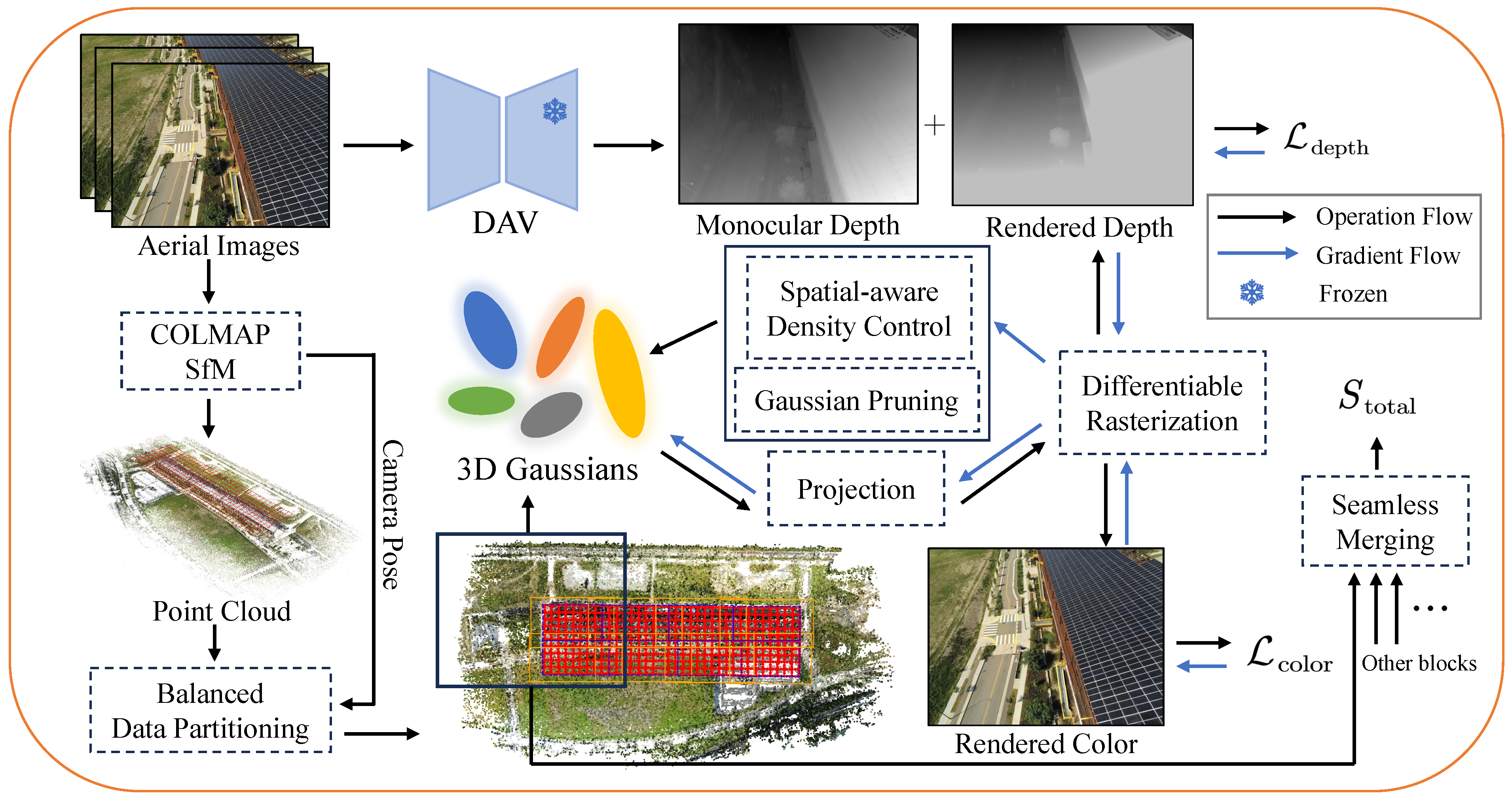
Our pipeline processes aerial images through COLMAP [32] reconstruction, scene partitioning with Balanced Data Partitioning, depth supervision from a frozen monocular depth network, Spatial-aware Density Control, and Gaussian Pruning, ultimately merging partitions for a unified, efficient scene representation. The overview of the entire framework is shown in Figure 1.

3.1. Preliminary

3D Gaussian Splatting (3DGS). 3DGS represents a 3D scene as a set of ellipsoidal Gaussians $\mathcal{G}=\left\{{\mathit{G}}_n\mid n=1,\dots ,N\right\}$. Each Gaussian ${\mathit{G}}_n$ is defined by a central point ${\mathit{\mu }}_{\mathit{n}}\in {\mathbb{R}}^{3\times 1}$, covariance ${\mathit{\Sigma }}_{\mathit{n}}\in {\mathbb{R}}^{3\times 3}$, opacity ${\sigma }_n\in \left[0,1\right]$, and spherical harmonic (SH) features ${\mathit{f}}_{\mathit{n}}\in {\mathbb{R}}^{3\times 16}$ for view-dependent rendering. The covariance matrix ${\mathit{\Sigma }}_{\mathit{n}}$ is factorized into a scaling matrix ${\mathit{R}}_{\mathit{n}}$ and a rotation matrix ${\mathit{S}}_{\mathit{n}}$, such that ${\mathit{\Sigma }}_{\mathit{n}}={\mathit{R}}_{\mathit{n}}{\mathit{S}}_{\mathit{n}}{\mathit{S}}_{\mathit{n}}^T{\mathit{R}}_{\mathit{n}}^T$.

For rendering, the color at a pixel p is calculated through alpha blending, where the contribution from each intersecting Gaussian ${\mathit{G}}_i$ is computed as follows:

$${\mathit{c}}_p=\sum _{i\in r\left(p\right)}{\mathit{c}}_i{\alpha }_i\prod _{j=1}^{i-1}(1-{\alpha }_j).$$

(1)

Here, $r\left(p\right)$ denotes the Gaussians along the ray passing through pixel p, and ${\alpha }_i$ is the opacity of each Gaussian, which depends on the query point x and the Gaussian parameters:

$${\alpha }_i={\sigma }_{i}exp\left(-{\displaystyle \frac{1}{2}}{(\mathit{x}-{\mathit{\mu }}_i)}^T{\mathit{\Sigma }}_{\mathit{i}}^{-1}(\mathit{x}-{\mathit{\mu }}_i)\right).$$

(2)

The optimization of the Gaussians is supervised by a combined loss function, which includes $L_1$ and D-SSIM losses, guiding the model to minimize the reconstruction error between the rendered and target images:

$$\mathcal{L}=(1-\lambda ){\mathcal{L}}_1(I_r,I_t)+\lambda {\mathcal{L}}_{\mathrm{D}-\mathrm{SSIM}}(I_r,I_t),$$

(3)

where $I_r$ is the rendered image, $I_t$ is the target image, and $\lambda$ is a hyperparameter that controls the weighting between the $L_1$ and D-SSIM losses.

3.2. Balanced Data Partitioning

Vanilla 3DGS uses millions of explicit 3D Gaussian ellipsoids as primitives to depict a large-scale 3D scene, which can consume a large amount of GPU memory (VRAM). To address this issue, we adopt a block-wise partitioning strategy similar to that in References [13,15] to divide the scene into smaller overlapping regions for parallel optimization.

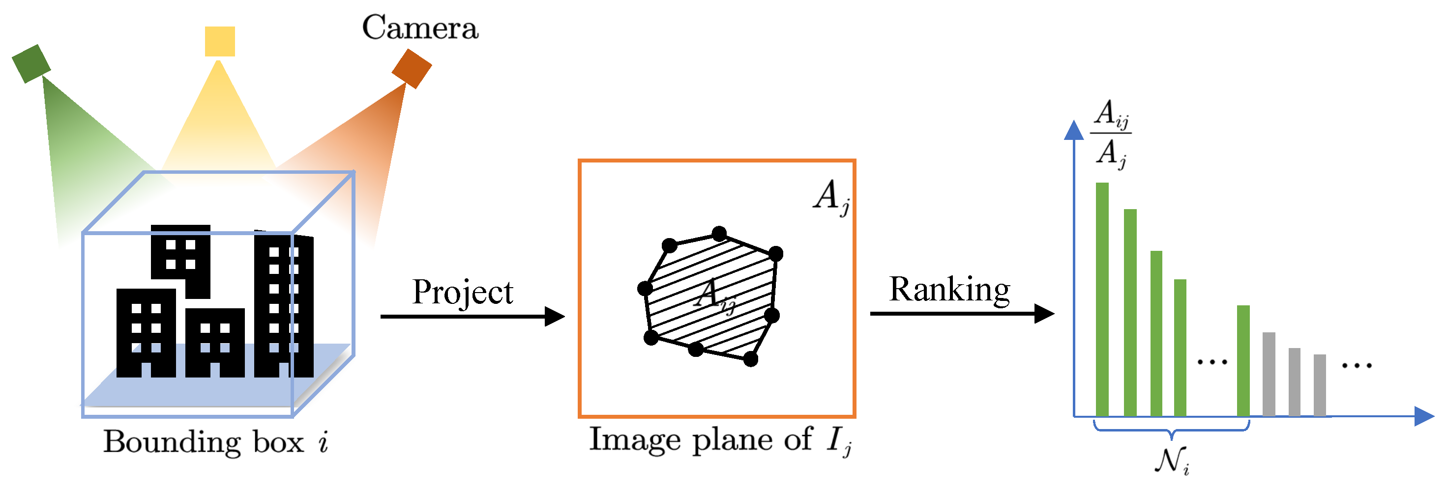
Given a sparse point cloud P and camera poses $\mathcal{T}=\left\{T_i\mid i\in 1,2\dots N\right\}$, which are generated by COLMAP [32] from a collection of images $\mathcal{I}=\left\{I_i\mid i\in 1,2\dots N\right\}$, we divide the scene into $m\times n$ blocks based on camera positions. In order to increase the overlap between adjacent blocks and minimize artifacts across the scene, we extend the boundaries of each block by a certain proportion (default 0.2). To further improve the reconstruction fidelity of each block, we introduce the visibility-based camera selection in [13] to add more relevant cameras for each block. The visibility score of the block i with respect to the camera j is defined as $A_{ij}/A_j$, where $A_{ij}$ represents the convex hull area of the block i projected onto the image $I_j$, and $A_j$ is the area of image $I_j$. Only cameras with visibility scores greater than the threshold ${\tau }_s$ will be selected.

However, this selection strategy will increase the imbalance in the number of cameras between blocks, resulting in larger blocks requiring greater VRAM consumption and a longer training time during parallel training, affecting the final training efficiency. Therefore, we develop a balanced data strategy to solve this problem, as shown in Figure 2. Specifically, we compute the visibility scores of block i for cameras in all other blocks and introduce a variable parameter ${\mathcal{N}}_i$ to control the number of selected cameras based on the number of point cloud points $P_i$ in the current block:

$${\mathcal{N}}_i={\mathcal{N}}_{min}+\left({\mathcal{N}}_{max}-{\mathcal{N}}_{min}\right)·\left(1-{\displaystyle \frac{log\left(P_i+1\right)}{log\left(P_{max}+1\right)}}\right),$$

(4)

where ${\mathcal{N}}_{min}$ and ${\mathcal{N}}_{max}$ are hyperparameters adjusted based on the total number of cameras, and $P_{max}$ represents the maximum number of point clouds in all blocks. For each block, the top ${\mathcal{N}}_i$ images with the highest scores are selected as viewpoints to optimize the data block.

3.3. Spatially Aware Density Control

To address the issue of blur and artifacts that are prone to occur during large-scene rendering, mainly due to the sparse initial point cloud in some regions, we propose a spatially aware densification strategy for large scenes. 3DGS [12] applies adaptive density control to prevent under- or over-reconstruction, which is guided by the average magnitude of view-space positional gradients. Specifically, for Gaussian ${\mathit{G}}_i$, under viewpoint k, the pixel-space coordinates of the projection point are ${\mu }^{i,k}=\left({\mu }_x^{i,k},{\mu }_y^{i,k}\right)$ and the corresponding loss is $L_k$. Thus, the average view-space positional gradients can be computed as follows:

$${\nabla }_{densify}={\displaystyle \frac{{\sum }_{k=1}^M\sqrt{{\left(\frac{\partial L_k}{\partial {\mu }_x^{i,k}}\right)}^2+{\left(\frac{\partial L_k}{\partial {\mu }_y^{i,k}}\right)}^2}}{M}},$$

(5)

when ${\nabla }_{densify}>{\tau }_g$, where ${\tau }_g$ is the gradient threshold (set to 0.002 by default), the Gaussian ${\mathit{G}}_i$ will be transformed into two Gaussians to populate empty areas.

AbsGS [34] proposed the theory of gradient collision to prove that the above strategy ignores that the per-pixel gradient ${\displaystyle \frac{\partial L_k}{\partial {\mu }_x^{i,k}}}$ (as well as ${\displaystyle \frac{\partial L_k}{\partial {\mu }_y^{i,k}}}$) may have different directions for different view-space pixels covered by ${\mathit{G}}_i$, causing the accumulated gradient to fail to reach the threshold. To solve this, we adopt the homodirectional gradient put forward by AbsGS, which is calculated by the following:

$${\displaystyle \frac{\partial L_k}{\partial {\mu }_x^{i,k}}}=\sum _{j=1}^m\left|{\displaystyle \frac{\partial L_k^j}{\partial {\mu }_x^{i,k}}}\right|,{\displaystyle \frac{\partial L_k}{\partial {\mu }_y^{i,k}}}=\sum _{j=1}^m\left|{\displaystyle \frac{\partial L_k^j}{\partial {\mu }_y^{i,k}}}\right|.$$

(6)

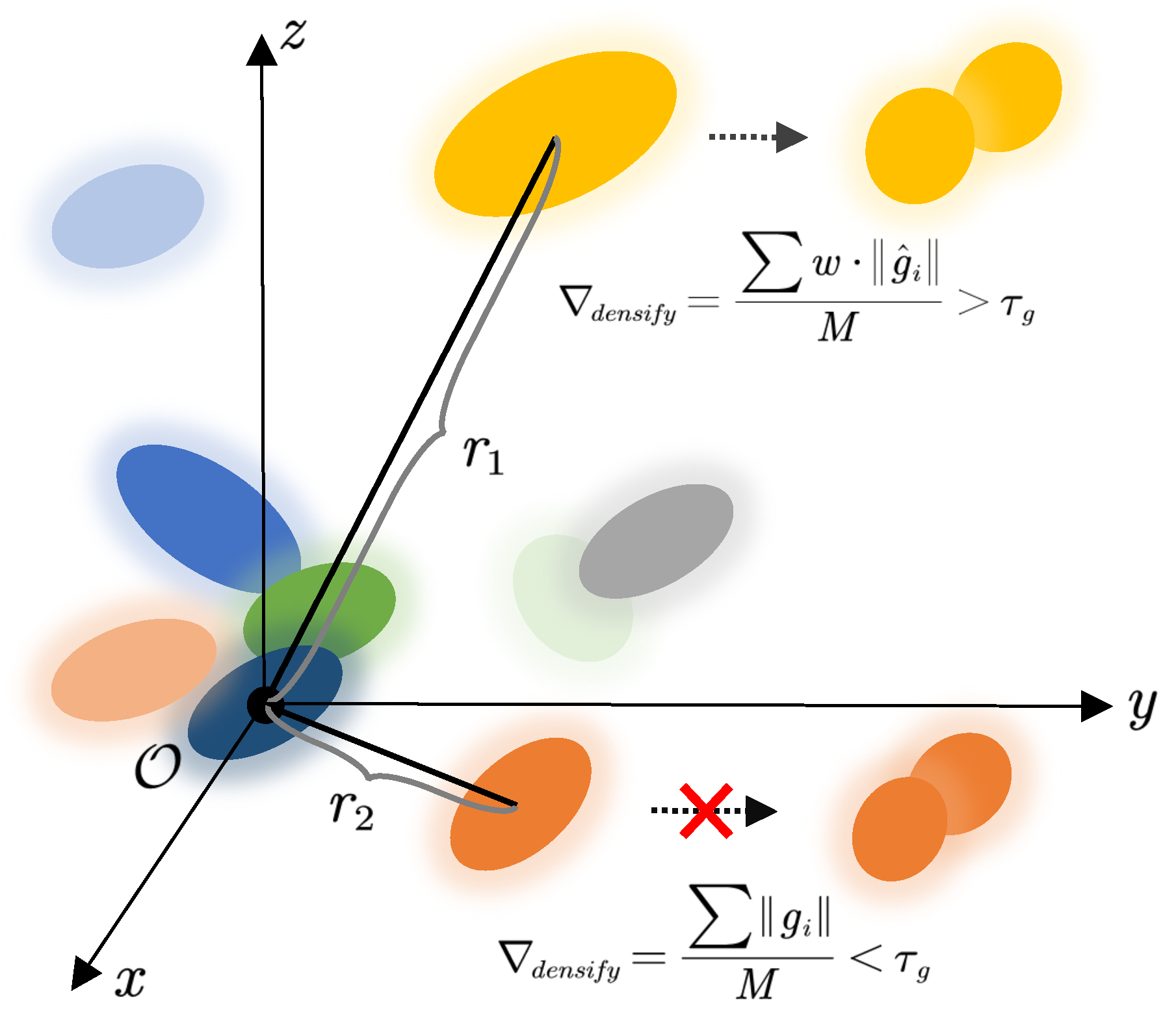
But, for large-scale scene reconstruction, we are more concerned with the quality of faraway objects, which are more prone to blurring artifacts, rather than over-abusing the densification strategy, which can easily lead to out-of-memory problems. Additionally, Gaussian growth will accelerate the generation of floaters near the camera, affecting rendering quality. Inspired by [35,36], we assign a weight w to the average view-space positional gradients:

$$w(i,k)=\left\{\begin{array}{cc}1\hfill & \mathrm{if}{∥{\mu }_{i,k}∥}_2<2r\hfill \\ {∥{\mu }_{i,k}∥}_2/\mathrm{r}-1\hfill & \mathrm{if}{∥{\mu }_{i,k}∥}_2⩾2r,\hfill \end{array}\right.$$

(7)

where ${\mu }_{i,k}$ is the mean vecter(position) for Gaussian ${\mathit{G}}_i$ under viewpoint k, indicating the distance between the point and the center of the scene, and r denotes the scene radius, which is calculated by the following:

$$r=1.1·\underset{i}{max}\left\{{∥{\mathit{C}}_i-{\displaystyle \frac{1}{N}}\sum _{j=1}^N{\mathit{C}}_i∥}_2\right\},$$

(8)

where N and ${\mathit{C}}_i$ represent the total number of training viewpoints and the world coordinates of the j-th viewpoint’s camera. Therefore, our spatially aware density control is determined by the following:

$${\nabla }_{densify}={\displaystyle \frac{{\sum }_{k=1}^{M}w\left(i,k\right)·\sqrt{{\left(\frac{\partial L_k}{\partial {\mu }_x^{i,k}}\right)}^2+{\left(\frac{\partial L_k}{\partial {\mu }_y^{i,k}}\right)}^2}}{M}}>{\tau }_g.$$

(9)

It should be noted that the homodirectional gradient in this formula is used only when ${∥{\mu }_{i,k}∥}_2⩾2r$. In this way, we can control distant points to be more easily densified without increasing the memory consumption caused by the densification of nearby Gaussian spheres, as illustrated in Figure 3.

3.4. Gaussian Pruning

Vanilla 3DGS reduces the density of Gaussians by pruning and resetting the opacity, specifically removing Gaussians with low opacity values based on a threshold ${ϵ}_{\alpha }$ during optimization. However, using opacity alone to estimate Gaussian importance might mistakenly remove a considerable number of significant Gaussians, especially for large scenes, resulting in poor reconstruction. Inspired by Equation (1), we use the blending weight ${\alpha }_i{\prod }_{j=1}^{i-1}\left(1-{\alpha }_j\right)$ to evaluate the Gaussian’s contribution to a pixel along the ray r. The total contribution of a Gaussian to the k-th rendered image can be calculated as follows:

$$\begin{array}{cc}\hfill & {\mathit{S}}_i=\sum _{r\in {\mathbb{R}}_k}{\alpha }_{i\left(r\right)}·\left(\prod _{j=1}^{i\left(r\right)-1}\left(1-{\alpha }_j\right)\right)·\gamma \left(\mathit{\Sigma }\right),\hfill \\ \hfill & \gamma \left(\mathit{\Sigma }\right)={\left(V_{\mathrm{norm}}\right)}^{\beta },\hfill \\ \hfill & V_{\mathrm{norm}}=min\left({\displaystyle \frac{V\left(\mathit{\Sigma }\right)}{V_{max90}}},1\right),\hfill \end{array}$$

(10)

where ${\mathbb{R}}_k$ denotes the set of rays that intersect the corresponding Gaussian from certain pixels. The important score also uses the adjusted 3D Gaussian volume $\gamma \left(\mathit{\Sigma }\right)$ [25] as the weight in order to prune Gaussians more flexibly for different volumes. The Gaussian volume is normalized by the largest $90\%$ of all sorted Gaussians, and the range is clamped between 0 and 1. Hyperparameter $\beta$ is introduced to control the weight.

In this way, we select several images with the highest Gaussian contribution score as the final score:

$$\mathit{S}={\displaystyle \frac{1}{\mathbb{V}}}\sum _{k\in \mathbb{V}}{\mathit{S}}_k,$$

(11)

where $\mathbb{V}$ is the set of images with the highest score. During training, we sort the final contribution values of all Gaussians and remove a specific percentage of Gaussians with the lowest contribution values, which can significantly reduce VRAM consumption and model storage.

3.5. Training Procedure

For large scenes, it is not realistic to use the photometric loss over full resolution images to learn the complex details of the environment early in the training, since the Gaussians are coarsely initialized from the sparse point cloud. In the early training stage, we adopt the Coarse-to-Fine strategy used in EAGLES [26], which progressively increases the image resolution to help to learn finer details of the scene and shorten the training time. To enhance the structural consistency of the reconstructed scene geometry, we use the depth priors generated by a scale-aligned pretrained monocular depth model during optimization with each input image. We introduce a depth regularization loss based on Pearson correlation. In contrast to conventional pixel-wise losses, this approach emphasizes the preservation of relative depth relationships rather than absolute value matching. This property makes it particularly effective when leveraging monocular depth priors, which often suffer from global scale ambiguity. The loss function of depth regularization is defined as follows:

$${\mathcal{L}}_{\mathrm{depth}}={\lambda }_d\sum {∥{\displaystyle \frac{\mathrm{Cov}\left(D,\widehat{D}\right)}{\sqrt{\mathrm{Var}\left(D\right)\mathrm{Var}\left(\widehat{D}\right)}}}∥}_1,$$

(12)

where ${\lambda }_d$ is the loss weight that continuously decays with the number of iterations, $\widehat{D}$ is the rendered inverse depth map, and D is the monocular depth. $\mathrm{Cov}\left(·\right)$ and $\mathrm{Var}\left(·\right)$ denote the covariance and variance operators respectively. Finally, the total training loss can be summarized as follows:

$$\mathcal{L}=(1-\lambda ){\mathcal{L}}_1(I_r,I_t)+\lambda {\mathcal{L}}_{\mathrm{D}-\mathrm{SSIM}}(I_r,I_t)+{\mathcal{L}}_{\mathrm{depth}}.$$

(13)

4. Experiments

4.1. Experimental Setup

Dataset and Metrics. We evaluated our proposed method on five large-scale scenes: Building and Rubble from Mill19 [7], Residence and Sci-Art from UrbanScene3D [37], and Aerial from a small city within the MatrixCity [38] dataset. Each of these datasets was collected using drones, with every scene containing thousands of high-resolution images. We downsampled all the images by 4 times from the original resolution during training and evaluation, except for the MatrixCity dataset, following previous work [13,15,16] for fair comparison. We evaluated the quality of novel view synthesis using PSNR, SSIM [39] and LPIPS [40] metrics.

Implementations and Baselines. We compared our method with NeRF-based methods: Mega-NeRF [7], Switch-NeRF [8], and 3DGS-based methods: 3DGS [12], VastGaussian [13], CityGaussian [15], DOGS [14], Momentum-GS [16]. We divided all scenes into 8 blocks and increased the total number of training iterations to 60,000. To provide a trade off between densification and VRAM requirements, Spatial-aware Density Control startsed at 10,000 iterations and ended at 40,000 iterations, with an interval of 200 iterations, the same as that described in [13]. We performed the proposed pruning operation at fixed intervals of 4000 training iterations. During the first 30,000 training iterations, we employed a cosine annealing schedule to progressively adjust the image resolution, gradually increasing the downsampling rate from 0.3 to 1.0. We adopted Depth-Anything-V2 [33] as the monocular depth estimation model. All experiments were conducted on 8 NVIDIA RTX 4090 GPUs (manufactured by NVIDIA, Santa Clara, CA, USA).

4.2. Results Analysis

In

Table 1. Quantitative comparison of our method with previous work on five large-scale scenes. We present metrics for PSNR ↑, SSIM ↑, and LPIPS ↓ on test views. ^† denotes without applying the decoupled appearance encoding, ‘-’ symbol indicates that Mega-NeRF and Switch-NeRF are not evaluated on MatrixCity due to the difficulty of training them under different configurations.

Method	Building			Rubble			Residence			Sci-Art			MatrixCity
	PSNR ↑	SSIM ↑	LPIPS ↓	PSNR ↑	SSIM ↑	LPIPS ↓	PSNR ↑	SSIM ↑	LPIPS ↓	PSNR ↑	SSIM ↑	LPIPS ↓	PSNR ↑	SSIM ↑	LPIPS ↓
Mega-NeRF [7]	20.93	0.547	0.504	24.06	0.553	0.516	22.08	0.628	0.489	25.60	0.770	0.390	-	-	-
Switch-NeRF [8]	21.54	0.579	0.474	24.31	0.562	0.496	22.57	0.654	0.457	26.52	0.795	0.360	-	-	-
3D-GS [12]	20.46	0.720	0.305	25.47	0.777	0.277	21.44	0.791	0.236	21.05	0.830	0.242	23.67	0.735	0.384
VastGaussian † [13]	21.80	0.728	0.225	25.20	0.742	0.264	21.01	0.699	0.261	22.64	0.761	0.261	28.33	0.835	0.220
CityGaussian [15]	21.55	0.778	0.246	25.77	0.813	0.228	22.00	0.813	0.211	21.39	0.837	0.230	27.46	0.865	0.204
DOGS [14]	22.73	0.759	0.204	25.78	0.765	0.257	21.94	0.740	0.244	24.42	0.804	0.219	28.58	0.847	0.219
Momentum-GS [16]	23.23	0.815	0.194	25.93	0.827	0.201	22.21	0.818	0.197	23.02	0.856	0.205	28.01	0.880	0.179
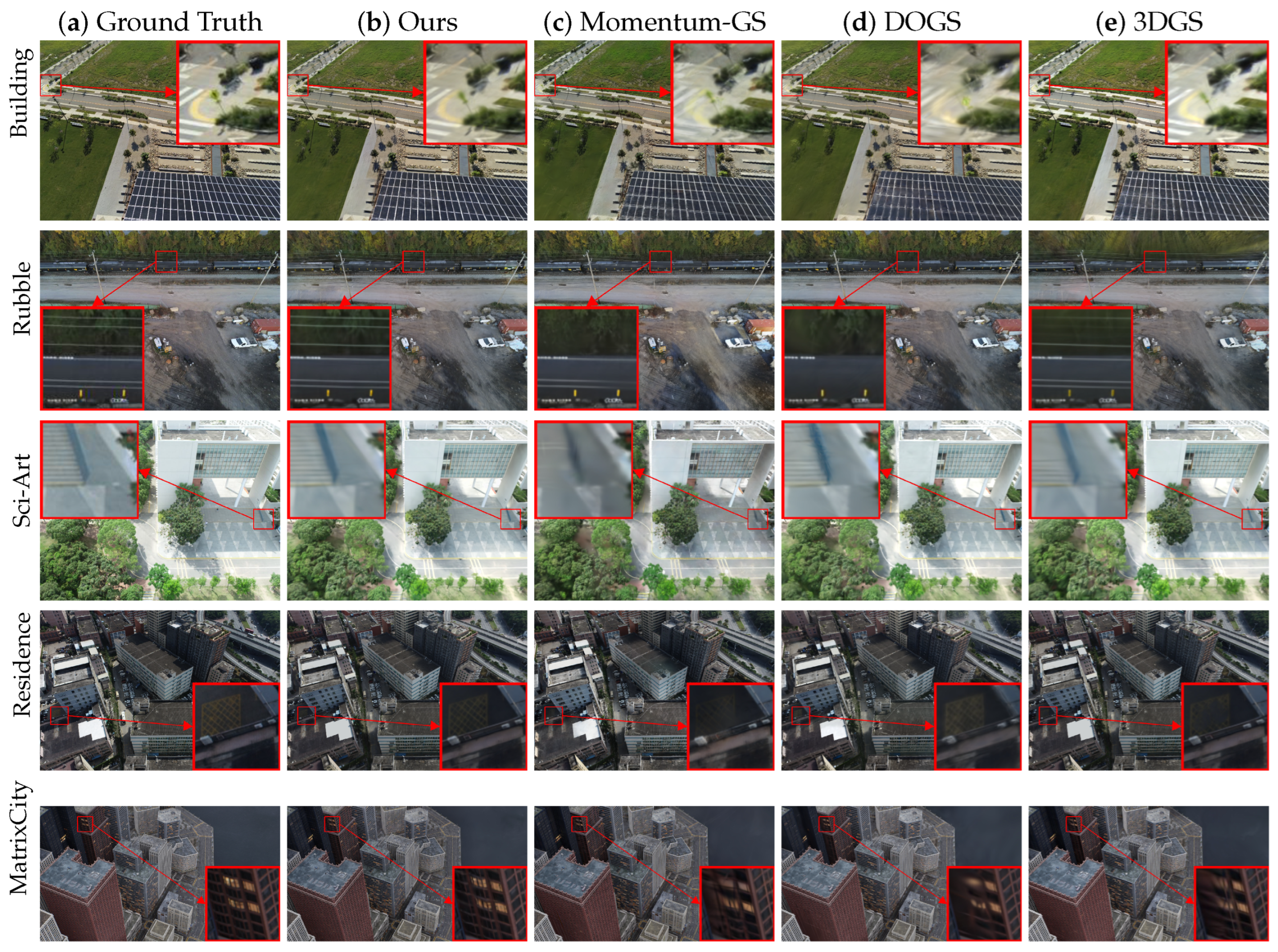
Ours	25.51	0.834	0.174	27.22	0.814	0.178	23.43	0.820	0.169	24.74	0.842	0.170	28.42	0.849	0.174

, we report the PSNR, SSIM, and LPIPS metrics across all large-scale scenes. The results demonstrate that our method achieves the best performance in almost all scenes. Notably, our method significantly outperforms several 3DGS-based methods on PSNR and LPIPS, highlighting the superior accuracy of our rendering strategy in capturing fine details and maintaining color consistency across complex scenes. However, on the Sci-Art dataset, NeRF-based methods achieve higher PSNR values compared to 3DGS-based methods. This can be attributed to the presence of overexposure and blur in many images within the dataset, which negatively impacts the reconstruction quality of 3DGS-based approaches. In Figure 4, we present visual comparisons that further validate the fidelity of our rendering quality. The visual results demonstrate that our method produces sharper textures, more accurate color reproduction, and better preservation of fine details compared to other methods. Notably, other methods tend to produce noticeable blurring and loss of detail in distant and complex regions, which further validates the effectiveness of our spatially aware densification strategy.

In

Table 2. Quantitative comparison of our method against previous work on four large-scale scenes. We report the training time (hh:mm), the number of final points (${10}^6$), and the storage size (GB).

Scenes	Building			Rubble			Residence			Sci-Art
	Times ↓	Points	Mem ↓	Times ↓	Points	Mem ↓	Times ↓	Points	Mem ↓	Times ↓	Points	Mem ↓
Mega-NeRF [7]	19:49	-	5.84	30:48	-	5.88	27:20	-	5.99	27:39	-	5.97
Switch-NeRF [8]	24:46	-	5.84	38.30	-	5.87	35:11	-	5.94	34:34	-	5.92
3D-GS [12]	21:37	7.99	4.62	18:40	3.85	2.18	23:13	5.35	3.23	21:33	2.31	1.61
DOGS [14]	03:51	6.89	3.39	02:25	4.74	2.54	04:33	7.64	6.11	04:23	5.67	3.53
Momentum-GS [16]	03:32	8.33	2.45	02:49	5.09	1.50	04:11	6.79	2.00	03:45	3.30	0.97
Ours	00:52	6.49	1.51	00:43	4.85	1.23	01:23	7.54	1.87	01:21	5.51	1.34

The arrow ↓ indicates that lower values are better. The symbol ‘-’ denotes that the metric is not applicable.

, we further compare the training time and model storage size across four representative datasets to assess the efficiency and compactness of our method. The results indicate that our method achieves superior rendering quality while simultaneously requiring less training time and producing a more compact model.

4.3. Ablation Study

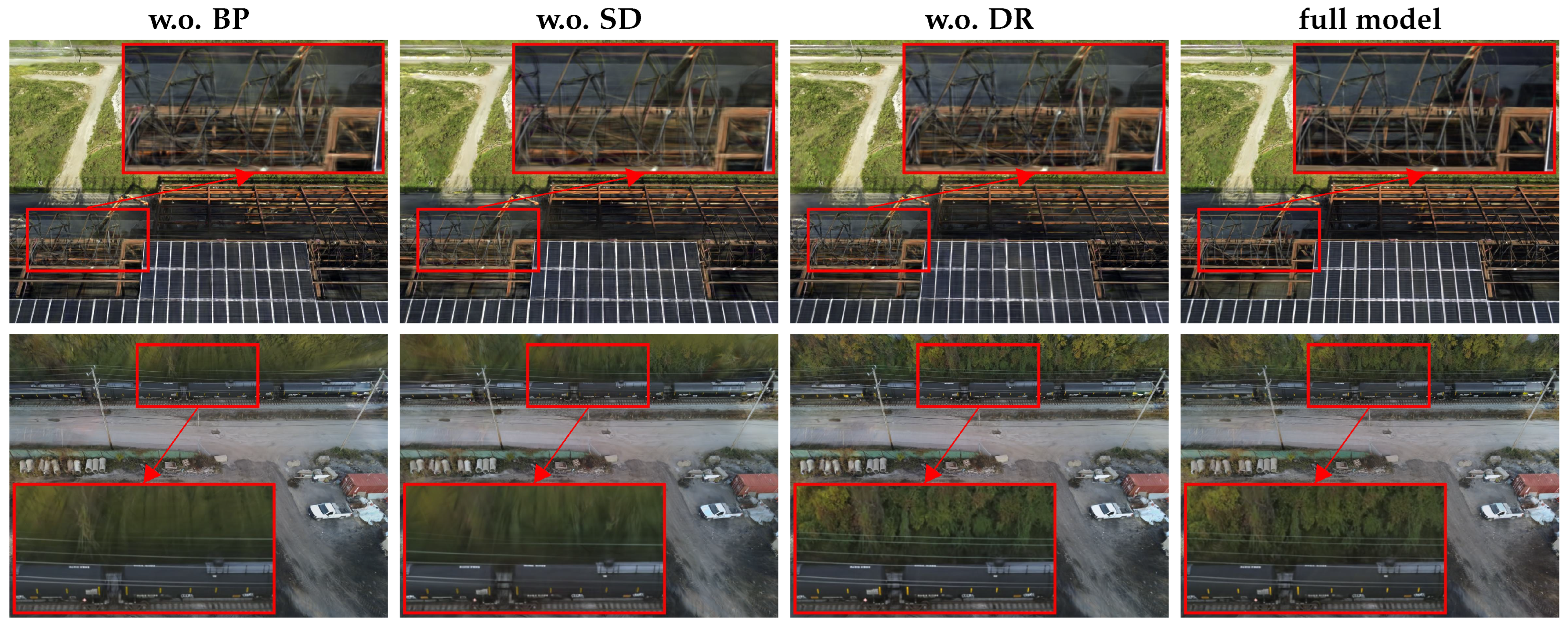
We conducted ablation experiments on the Building and Rubble datasets to evaluate the impact of each component in our method. Our method without balanced data partition is denoted as w.o. BP, the method without spatial-aware density control as w.o. SD, and the method without depth regularization as w.o. DR. The quantitative results in

Table 3. Ablation study of our method.

Scenes	Building			Rubble
	PSNR ↑	SSIM ↑	LPIPS ↓	PSNR ↑	SSIM ↑	LPIPS ↓
w.o. BP	21.74	0.732	0.223	24.72	0.745	0.237
w.o. SD	23.08	0.770	0.194	25.43	0.761	0.201
w.o. DR	25.31	0.816	0.186	26.81	0.792	0.182
full model	25.51	0.834	0.174	27.22	0.814	0.178

The arrow ↑ indicates that higher values are better, and ↓ indicates that lower values are better.

demonstrate the contribution of each module. As presented in the table, removing balanced data partition leads to incomplete training of individual scene blocks, leading to a substantial decline in performance metrics. Similarly, the performance without spatially aware densification deviates significantly from the full model, mainly due to the insufficient densification of distant objects, which results in noticeable blurring artifacts. We also provide quantitative results in Figure 5 to further illustrate this effect. The absence of depth regularization shows a minimal difference compared to the full model. However, as observed in the figure, the full model achieves superior rendering quality and preserves finer geometric details.

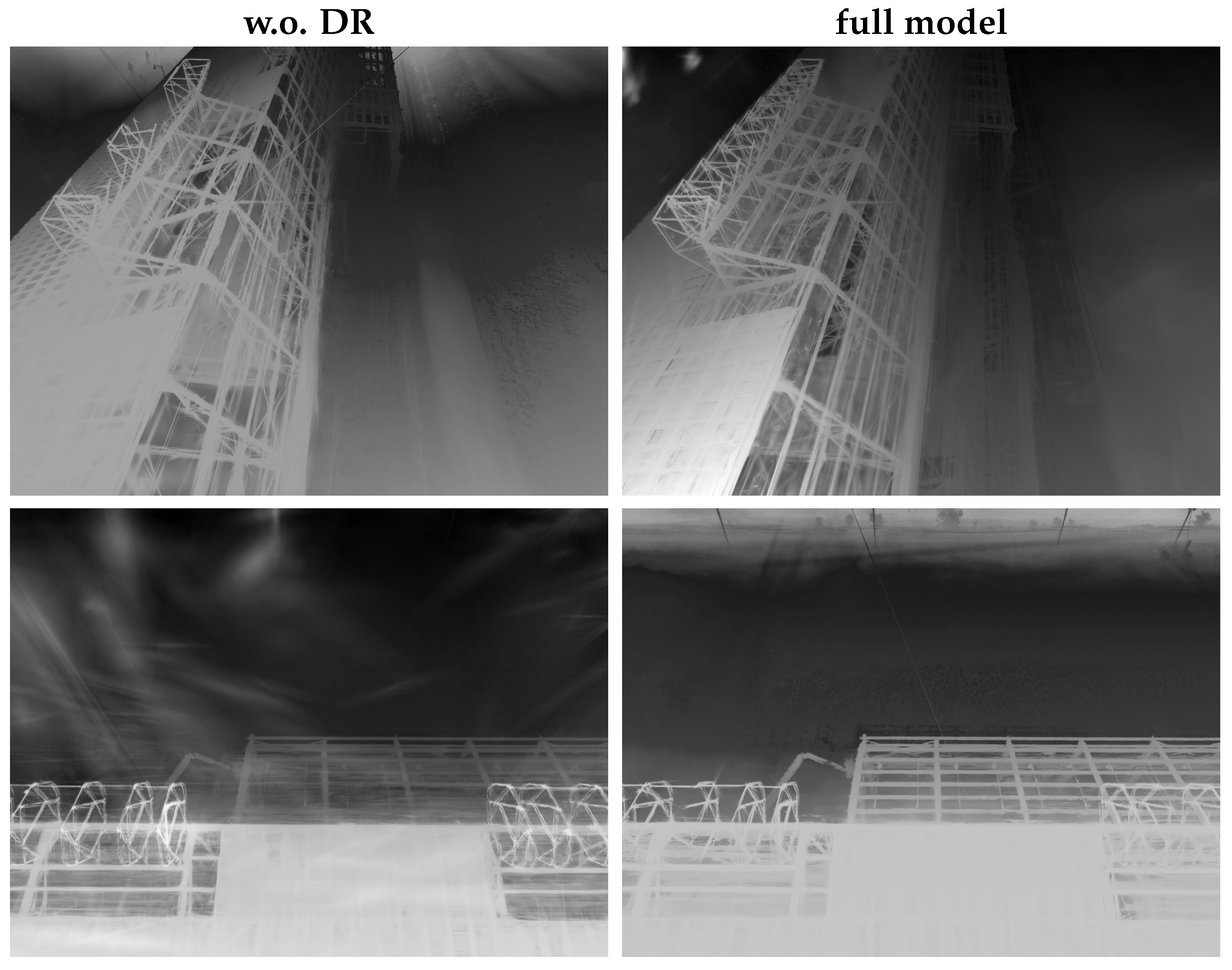
Furthermore, we visualize the specific impact of Depth Regularization (DR) in Figure 6. As illustrated, the rendered depth maps in the w.o. DR setting exhibit significant degradation compared to the full model, lacking geometric consistency. This geometric inaccuracy hinders the effective optimization of appearance, resulting in under-trained textures on building surfaces. In contrast, the inclusion of DR guides the geometry to be more plausible, thereby allowing the model to capture sharper and more accurate surface details. To validate dynamic weight scheduling for depth, we conducted a sensitivity analysis by comparing our exponential decay strategy against constant weighting schemes (Fixed-High and Fixed-Low). As shown in

Table 4. Ablation study of depth loss scheduling in our method.

	PSNR ↑	SSIM ↑	LPIPS ↓
Fixed High (1.0)	23.71	0.783	0.207
Fixed Low (0.01)	25.30	0.812	0.191
Decay	25.51	0.834	0.174

The arrow ↑ indicates that higher values are better, and ↓ indicates that lower values are better.

, our strategy yields the best trade-off between geometric accuracy and rendering quality. The results support our design rationale: in the early training phase, a stronger depth constraint is essential to accelerate geometric convergence and resolve scale ambiguities. However, since the depth maps from monocular estimators often contain noise or inaccuracies, enforcing a strong constraint throughout the entire optimization process restricts the model from refining high-frequency details and may introduce artifacts. Our proposed decay schedule successfully utilizes depth priors for initial guidance while mitigating the negative impact of depth inconsistencies during the fine-tuning stage, resulting in sharper rendering details.

Moreover, we present the pruning percentage in

Table 5. Ablation study of the pruning ratio in our method. We report the training time (hh:mm), the number of final points (${10}^6$), and the storage size (GB).

	PSNR ↑	SSIM ↑	LPIPS ↓	Times ↓	Points	Mem ↓
0	25.42	0.827	0.180	01:19	7.71	1.78
0.1	25.48	0.830	0.173	01:10	7.09	1.64
0.2	25.51	0.834	0.174	00:58	6.49	1.51
0.3	25.21	0.813	0.191	00:52	5.92	1.37

The arrow ↑ indicates that higher values are better, and ↓ indicates that lower values are better.

. When the pruning ratio is set to 0.2, our method achieves the best overall performance. In contrast, lower pruning ratios (e.g., 0 or 0.1) lead to suboptimal results, possibly due to the excessive density of low-contributing Gaussians, which may hinder the effective learning of a scene. Considering both reconstruction quality and resource efficiency, we adopted a pruning ratio of 0.2 in our experiments, as this offers the best trade-off.

5. Conclusions

In this paper, we propose an efficient and scalable framework for high-fidelity large-scale scene reconstruction based on 3D Gaussian Splatting. Our method introduces a visibility-based camera selection strategy with adaptive control to balance memory usage and reduce artifacts, a spatially aware densification scheme to enhance reconstruction quality for distant regions, and an improved pruning mechanism that accurately evaluates the contribution of each Gaussian. In addition, we incorporate a depth regularization loss based on Pearson correlation to enhance geometric consistency under scale ambiguity. Extensive experiments demonstrate that our approach achieves state-of-the-art results, offering superior rendering quality and training efficiency across diverse scenes.

Beyond quantitative improvements, our framework also exhibits strong practicality and adaptability, making it well-suited for real-world applications such as autonomous driving, digital twin construction, large-scale urban modeling, and immersive virtual reality content generation. In future work, we aim to further accelerate both training and novel view synthesis by adopting more compact model compression strategies and optimized parallelization techniques. Moreover, we plan to integrate our method into downstream tasks such as large-scale orthophoto generation and scene understanding for autonomous driving, bridging high-fidelity 3D reconstruction with broader practical utility.

References

1. Yang, Z.; Chai, Y.; Anguelov, D.; Zhou, Y.; Sun, P.; Erhan, D.; Rafferty, S.; Kretzschmar, H. Surfelgan: Synthesizing realistic sensor data for autonomous driving. In Proceedings of the IEEE/CVF Conference on Computer Vision and Pattern Recognition, Seattle, WA, USA, 14–19 June 2020; pp. 11118–11127. [Google Scholar]
2. Ost, J.; Mannan, F.; Thuerey, N.; Knodt, J.; Heide, F. Neural scene graphs for dynamic scenes. In Proceedings of the IEEE/CVF Conference on Computer Vision and Pattern Recognition, Nashville, TN, USA, 19–25 June 2021; pp. 2856–2865. [Google Scholar]
3. Yan, Y.; Lin, H.; Zhou, C.; Wang, W.; Sun, H.; Zhan, K.; Lang, X.; Zhou, X.; Peng, S. Street gaussians: Modeling dynamic urban scenes with gaussian splatting. In European Conference on Computer Vision; Springer: Berlin/Heidelberg, Germany, 2024; pp. 156–173. [Google Scholar]
4. Zhou, X.; Lin, Z.; Shan, X.; Wang, Y.; Sun, D.; Yang, M.H. Drivinggaussian: Composite gaussian splatting for surrounding dynamic autonomous driving scenes. In Proceedings of the IEEE/CVF Conference on Computer Vision and Pattern Recognition, Seattle, WA, USA, 17–18 June 2024; pp. 21634–21643. [Google Scholar]
5. Jiang, Y.; Yu, C.; Xie, T.; Li, X.; Feng, Y.; Wang, H.; Li, M.; Lau, H.; Gao, F.; Yang, Y.; et al. Vr-gs: A physical dynamics-aware interactive gaussian splatting system in virtual reality. In ACM SIGGRAPH 2024 Conference Papers; ACM: New York, NY, USA, 2024; pp. 1–11. [Google Scholar]
6. Bozcan, I.; Kayacan, E. Au-air: A multi-modal unmanned aerial vehicle dataset for low altitude traffic surveillance. In Proceedings of the 2020 IEEE International Conference on Robotics and Automation (ICRA), Paris, France, 31 May–31 August 2020; pp. 8504–8510. [Google Scholar]
7. Turki, H.; Ramanan, D.; Satyanarayanan, M. Mega-NERF: Scalable Construction of Large-Scale NeRFs for Virtual Fly-Throughs. In Proceedings of the IEEE/CVF Conference on Computer Vision and Pattern Recognition (CVPR), New Orleans, LA, USA, 18–24 June 2022; pp. 12922–12931. [Google Scholar]
8. Mi, Z.; Xu, D. Switch-NeRF: Learning Scene Decomposition with Mixture of Experts for Large-scale Neural Radiance Fields. In Proceedings of the International Conference on Learning Representations (ICLR), Kigali, Rwanda, 1–5 May 2023. [Google Scholar]
9. Tancik, M.; Casser, V.; Yan, X.; Pradhan, S.; Mildenhall, B.; Srinivasan, P.P.; Barron, J.T.; Kretzschmar, H. Block-nerf: Scalable large scene neural view synthesis. In Proceedings of the IEEE/CVF Conference on Computer Vision and Pattern Recognition, New Orleans, LA, USA, 18–24 June 2022; pp. 8248–8258. [Google Scholar]
10. Martin-Brualla, R.; Radwan, N.; Sajjadi, M.S.M.; Barron, J.T.; Dosovitskiy, A.; Duckworth, D. NeRF in the Wild: Neural Radiance Fields for Unconstrained Photo Collections. In Proceedings of the IEEE/CVF Conference on Computer Vision and Pattern Recognition, Nashville, TN, USA, 19–25 June 2021. [Google Scholar]
11. Mildenhall, B.; Srinivasan, P.P.; Tancik, M.; Barron, J.T.; Ramamoorthi, R.; Ng, R. Nerf: Representing scenes as neural radiance fields for view synthesis. Commun. ACM 2021, 65, 99–106. [Google Scholar] [CrossRef] [Scilit]
12. Kerbl, B.; Kopanas, G.; Leimkühler, T.; Drettakis, G. 3d gaussian splatting for real-time radiance field rendering. ACM Trans. Graph. 2023, 42, 139:1–139:15. [Google Scholar] [CrossRef] [Scilit]
13. Lin, J.; Li, Z.; Tang, X.; Liu, J.; Liu, S.; Liu, J.; Lu, Y.; Wu, X.; Xu, S.; Yan, Y.; et al. VastGaussian: Vast 3D Gaussians for Large Scene Reconstruction. In Proceedings of the IEEE/CVF Conference on Computer Vision and Pattern Recognition, Seattle, WA, USA, 17–18 June 2024. [Google Scholar]
14. Chen, Y.; Lee, G.H. DOGS: Distributed-Oriented Gaussian Splatting for Large-Scale 3D Reconstruction Via Gaussian Consensus. arXiv 2024, arXiv:2400.00000. [Google Scholar]
15. Liu, Y.; Luo, C.; Fan, L.; Wang, N.; Peng, J.; Zhang, Z. Citygaussian: Real-time high-quality large-scale scene rendering with gaussians. In European Conference on Computer Vision; Springer: Berlin/Heidelberg, Germany, 2024; pp. 265–282. [Google Scholar]
16. Fan, J.; Li, W.; Han, Y.; Tang, Y. Momentum-GS: Momentum Gaussian Self-Distillation for High-Quality Large Scene Reconstruction. arXiv 2024, arXiv:2412.04887. [Google Scholar]
17. Fridovich-Keil, S.; Yu, A.; Tancik, M.; Chen, Q.; Recht, B.; Kanazawa, A. Plenoxels: Radiance Fields without Neural Networks. In Proceedings of the IEEE/CVF Conference on Computer Vision and Pattern Recognition, New Orleans, LA, USA, 18–24 June 2022. [Google Scholar]
18. Müller, T.; Evans, A.; Schied, C.; Keller, A. Instant neural graphics primitives with a multiresolution hash encoding. ACM Trans. Graph. 2022, 41, 1–15. [Google Scholar] [CrossRef] [Scilit]
19. Yariv, L.; Hedman, P.; Reiser, C.; Verbin, D.; Srinivasan, P.P.; Szeliski, R.; Barron, J.T.; Mildenhall, B. Bakedsdf: Meshing neural sdfs for real-time view synthesis. In ACM SIGGRAPH 2023 Conference Proceedings; ACM: New York, NY, USA, 2023; pp. 1–9. [Google Scholar]
20. Sun, C.; Sun, M.; Chen, H.-T. Direct voxel grid optimization: Super-fast convergence for radiance fields reconstruction. In Proceedings of the IEEE/CVF Conference on Computer Vision and Pattern Recognition, New Orleans, LA, USA, 18–24 June 2022; pp. 5459–5469. [Google Scholar]
21. Reiser, C.; Peng, S.; Liao, Y.; Geiger, A. Kilonerf: Speeding up neural radiance fields with thousands of tiny mlps. In Proceedings of the IEEE/CVF International Conference on Computer Vision, Montreal, BC, Canada, 11–17 October 2021; pp. 14335–14345. [Google Scholar]
22. Yu, Z.; Chen, A.; Huang, B.; Sattler, T.; Geiger, A. Mip-splatting: Alias-free 3d gaussian splatting. In Proceedings of the IEEE/CVF Conference on Computer Vision and Pattern Recognition, Seattle, WA, USA, 16–22 June 2024; pp. 19447–19456. [Google Scholar]
23. Lu, T.; Yu, M.; Xu, L.; Xiangli, Y.; Wang, L.; Lin, D.; Dai, B. Scaffold-gs: Structured 3d gaussians for view-adaptive rendering. In Proceedings of the IEEE/CVF Conference on Computer Vision and Pattern Recognition, Seattle, WA, USA, 17–18 June 2024; pp. 20654–20664. [Google Scholar]
24. Navaneet, K.L.; Meibodi, K.P.; Koohpayegani, S.A.; Pirsiavash, H. CompGS: Smaller and Faster Gaussian Splatting with Vector Quantization. In European Conference on Computer Vision; Springer: Berlin/Heidelberg, Germany, 2024. [Google Scholar]
25. Fan, Z.; Wang, K.; Wen, K.; Zhu, Z.; Xu, D.; Wang, Z. LightGaussian: Unbounded 3D Gaussian Compression with 15x Reduction and 200+ FPS. arXiv 2023, arXiv:2311.17245. [Google Scholar]
26. Girish, S.; Gupta, K.; Shrivastava, A. Eagles: Efficient accelerated 3d gaussians with lightweight encodings. In European Conference on Computer Vision; Springer: Berlin/Heidelberg, Germany, 2024; pp. 54–71. [Google Scholar]
27. Lee, J.C.; Rho, D.; Sun, X.; Ko, J.H.; Park, E. Compact 3D Gaussian Representation for Radiance Field. In Proceedings of the IEEE/CVF Conference on Computer Vision and Pattern Recognition (CVPR), Seattle, WA, USA, 16–22 June 2024; pp. 21719–21728. [Google Scholar]
28. Fan, L.; Yang, Y.; Li, M.; Li, H.; Zhang, Z. Trim 3D Gaussian Splatting for Accurate Geometry Representation. arXiv 2024, arXiv:2406.07499. [Google Scholar] [CrossRef] [Scilit]
29. Rematas, K.; Liu, A.; Srinivasan, P.P.; Barron, J.T.; Tagliasacchi, A.; Funkhouser, T.; Ferrari, V. Urban radiance fields. In Proceedings of the IEEE/CVF Conference on Computer Vision and Pattern Recognition, New Orleans, LA, USA, 18–24 June 2022; pp. 12932–12942. [Google Scholar]
30. Xu, L.; Xiangli, Y.; Peng, S.; Pan, X.; Zhao, N.; Theobalt, C.; Dai, B.; Lin, D. Grid-guided neural radiance fields for large urban scenes. In Proceedings of the IEEE/CVF Conference on Computer Vision and Pattern Recognition, Vancouver, BC, Canada, 18–22 June 2023; pp. 8296–8306. [Google Scholar]
31. Kerbl, B.; Meuleman, A.; Kopanas, G.; Wimmer, M.; Lanvin, A.; Drettakis, G. A hierarchical 3d gaussian representation for real-time rendering of very large datasets. ACM Trans. Graph. (TOG) 2024, 43, 1–15. [Google Scholar] [CrossRef] [Scilit]
32. Schönberger, J.L.; Frahm, J.-M. Structure-from-Motion Revisited. In Proceedings of the IEEE Conference on Computer Vision and Pattern Recognition, Las Vegas, NV, USA, 27–30 June 2016. [Google Scholar]
33. Yang, L.; Kang, B.; Huang, Z.; Zhao, Z.; Xu, X.; Feng, J.; Zhao, H. Depth anything v2. Adv. Neural Inf. Process. Syst. 2025, 37, 21875–21911. [Google Scholar]
34. Ye, Z.; Li, W.; Liu, S.; Qiao, P.; Dou, Y. Absgs: Recovering fine details in 3d gaussian splatting. In Proceedings of the 32nd ACM International Conference on Multimedia, Melbourne, VIC, Australia, 28 October–1 November 2024; pp. 1053–1061. [Google Scholar]
35. Chen, Y.; Gu, C.; Jiang, J.; Zhu, X.; Zhang, L. Periodic vibration gaussian: Dynamic urban scene reconstruction and real-time rendering. arXiv 2023, arXiv:2311.18561. [Google Scholar]
36. Zhang, Z.; Hu, W.; Lao, Y.; He, T.; Zhao, H. Pixel-gs: Density control with pixel-aware gradient for 3d gaussian splatting. In European Conference on Computer Vision; Springer: Berlin/Heidelberg, Germany, 2024; pp. 326–342. [Google Scholar]
37. Lin, L.; Liu, Y.; Hu, Y.; Yan, X.; Xie, K.; Huang, H. Capturing, Reconstructing, and Simulating: The UrbanScene3D Dataset. In European Conference on Computer Vision; Springer: Berlin/Heidelberg, Germany, 2022; pp. 93–109. [Google Scholar]
38. Li, Y.; Jiang, L.; Xu, L.; Xiangli, Y.; Wang, Z.; Lin, D.; Dai, B. Matrixcity: A large-scale city dataset for city-scale neural rendering and beyond. In Proceedings of the IEEE/CVF International Conference on Computer Vision, Paris, France, 2–6 October 2023; pp. 3205–3215. [Google Scholar]
39. Wang, Z.; Bovik, A.C.; Sheikh, H.R.; Simoncelli, E.P. Image quality assessment: From error visibility to structural similarity. IEEE Trans. Image Process. 2004, 13, 600–612. [Google Scholar] [CrossRef] [Scilit] [PubMed]
40. Zhang, R.; Isola, P.; Efros, A.A.; Shechtman, E.; Wang, O. The unreasonable effectiveness of deep features as a perceptual metric. In Proceedings of the IEEE Conference on Computer Vision and Pattern Recognition, Salt Lake City, UT, USA, 18–22 June 2018; pp. 586–595. [Google Scholar]
Figure 1. Overview of our framework. Our pipeline begins with aerial images, from which COLMAP [32] reconstructs a sparse point cloud and estimates camera poses. We apply Manhattan alignment to the point cloud and partition the scene based on camera poses using a Balanced Data Partitioning strategy that ensures uniform division for efficient parallel training. A frozen monocular depth network (DAV [33]) provides predicted depth maps, which are used to introduce a depth supervision loss for better geometric consistency. Three-dimensional Gaussians are optimized via differentiable rasterization, guided by both color and depth losses, while Spatial-aware Density Control and Gaussian Pruning are applied simultaneously to enhance scene details and manage computational cost. Finally, we seamlessly merge all partitions into a unified scene representation.
Applsci 16 00965 g001
Figure 2. Balanced camera selection strategy in a block. For each block, the visibility score is computed as the ratio between the projected area and the image area. The top N i images with the highest scores are selected as candidate viewpoints for that region.
Applsci 16 00965 g002
Figure 3. Illustration of our spatially aware densification strategy. In the original 3DGS method, densification is triggered based on the average view-space gradient g i = j L k j μ x i , k , j L k j μ y i , k , which may be suppressed due to conflicting gradient directions. To address this, we introduce a spatially weighted scheme where distant Gaussians are assigned higher weights, encouraging densification in regions prone to blur. Additionally, for points beyond 2 r , we apply homodirectional gradients g ^ i = j L k j μ x i , k , j L k j μ y i , k as proposed in AbsGS [34], ensuring that conflicting gradients do not cancel each other out. This approach enables detail-preserving densification for faraway objects while suppressing the excessive growth of nearby Gaussians to improve memory efficiency and reduce floaters.
Applsci 16 00965 g003
Figure 4. Qualitative comparisons of our method and prior methods across five large-scale scenes. The red insets mark regions where the visual differences between the methods are most pronounced.
Applsci 16 00965 g004
Figure 5. Ablation study of our method. (Top): the building dataset; (bottom): the rubble dataset.
Applsci 16 00965 g005
Figure 6. Ablation study of the depth regularization in our method.
Applsci 16 00965 g006