Pareto Local Search Guided by Archive Entropy

Abstract

Pareto local search (PLS) serves as an important component in multi-objective combinatorial optimization. Nevertheless, achieving a balance between convergence and diversity remains a challenge, as few studies have leveraged knowledge from the search archive to effectively guide the PLS process. This paper proposes an archive entropy-guided Pareto local search algorithm (AEG-PLS). In the proposed method, the objective space is partitioned into subregions using a set of reference vectors. The archive entropy is then computed for each subregion to assess population diversity. To enhance diversity in less explored areas, a PLS is initiated using a well-performing solution selected from the subregion with the lowest entropy, thus indicating the weakest diversity. This approach promotes a more balanced trade-off between convergence and diversity throughout the optimization process. Experimental results on 25 multi-objective combinatorial optimization benchmark instances demonstrate that the proposed AEG-PLS achieves competitive performance in terms of both Inverted Generational Distance and Hypervolume metrics when compared to nine state-of-the-art multi-objective evolutionary algorithms.

1. Introduction

Multi-objective combinatorial optimization problem (MCOP), a significant research topic within operations research, has broad applications in logistics scheduling, financial investment, and power systems [1,2]. These problems are characterized by a finite, discrete solution space and the need to simultaneously optimize multiple conflicting objectives [3,4]. Given the inherent conflicts between objectives, no single solution is optimal for all objectives, making the identification of the Pareto optimal set the primary goal [5,6,7]. Due to the exponential growth of the solution space with problem scale, these problems are typically NP-hard, and exact algorithms are only suitable for small-scale instances [8]. Therefore, solving practical problems largely relies on heuristic or meta-heuristic algorithms, particularly efficient approximation methods specifically designed for multi-objective optimization [9].

Given this context, heuristic and meta-heuristic methods have emerged as promising alternatives such that a key strategy they employ is the incorporation of local search mechanisms [10]. In single-objective combinatorial optimization, high-quality solutions are typically selected as the primary targets for local search exploration [11]. When extending this strategy to the multi-objective combinatorial optimization domain, a common approach is to focus the search on solutions stored within an archive, leading to the development of Pareto local search (PLS) [12], where exploration refers to the process of updating the archive by considering the neighboring solutions of the archived individuals.

However, traditional PLS and most of its variants struggle to dynamically guide the search direction using the information accumulated in the archive during the search process. This may cause the algorithm to prematurely converge to a local Pareto front or fail to achieve a uniform distribution along complex Pareto fronts. Therefore, the challenge of effectively extracting diversity-reflecting knowledge from the archive to dynamically steer the PLS search process, thereby achieving a better balance between convergence and diversity throughout the optimization, remains an open question worthy of in-depth research.

Inspired by the concept of entropy in information theory [13], this paper proposes an archive entropy-guided Pareto local search algorithm within the decomposition-based multi-objective evolutionary algorithm framework [14,15]. The core idea of the proposed algorithm is to identify regions with insufficient diversity as the most promising search directions. Specifically, the algorithm first divides the objective space into several subregions using a set of reference vectors. It then calculates the archive entropy of the solutions within each subregion, which serves as a quantitative indicator of the diversity richness in that area. The subregion with the lowest entropy value, that is, the region with the most deficient diversity, is prioritized as the next search direction. Finally, the algorithm selects a solution with good convergence from this region as a starting point to initiate a Pareto local search. This mechanism ensures that computational resources are dynamically and adaptively allocated to the areas most in need, thereby achieving a better trade-off between convergence and diversity throughout the optimization process.

The remainder of this paper is structured as follows. Section 2 reviews related work. Section 3 elaborates on the algorithmic framework and implementation details of AEG-PLS. Section 4 presents and discusses the experimental results. Finally, Section 5 concludes the paper and outlines directions for future research.

2. Preliminaries

Pareto local search (PLS) is a classic meta-heuristic algorithm [12,16,17] that progressively improves the quality of a solution set by exploring the neighborhood of each unexplored solution in an archive. It has been widely used to solve MCOPs [18,19,20]. In recent years, a growing body of research has focused on extending and enhancing PLS for complex MCOPs. For instance, Lust and Teghem [21] introduced a two-phase PLS approach that first constructs a high-quality initial population using prior techniques to better leverage the advantages of PLS. Building on the idea of two-phase local search, Dubois-Lacoste et al. [22] developed a hybrid PLS-based algorithm to address bi-objective flow-shop scheduling problems.

Despite these successful applications, a key challenge lies in the early-stage performance of PLS. Addressing this, Dubois-Lacoste et al. [18] argued that PLS is not always competitive before the termination condition is triggered and proposed some alternative replacements of the components in PLS to improve robustness. Based on the decomposition strategy, Dong et al. [23] proposed a dynamic local search based on the benefits brought by the optimization process of each subproblem. In a similar vein, Shi et al. [24,25] proposed a decomposition-based parallel PLS framework. To further improve information exchange and convergence speed across subregions, they incorporated a cooperative search mechanism and a dynamic subregion adjustment strategy that balances computational load by reallocating search areas [16]. Along another line of research, Cai et al. [26,27] proposed a constrained decomposition with grids method, which confines each subproblem to an independent grid cell, thereby ensuring the preservation of diverse solutions from different regions of the objective space and enabling their use as initial points for local search. Nevertheless, Cai et al. [28] integrated the NSGA-II [29] and MOEA/D [14] algorithms to propose an external archive-guided multi-objective evolutionary algorithm based on decomposition.

While these studies contribute to improving PLS performance, a more specific challenge in guiding PLS lies in the design of effective solution selection mechanisms. Although Jaszkiewicz [19,30] proposed a quality indicator based on the weighted Chebyshev function to address the issue of which solutions to explore within the PLS framework, the method remains limited by its lack of a search direction prioritization mechanism. This limitation may lead to the neglect of solutions that promote diversity, ultimately hindering the convergence to a well-distributed Pareto front. Previous studies [31,32,33,34] have emphasized that search-related information can play a critical role in guiding the optimization process. Nevertheless, while PLS deeply exploits high-quality solutions, that is, focusing primarily on convergence, few studies have explored how to explicitly use diversity as a form of search-related information to steer the PLS search trajectory.

3. Proposed Algorithm

The AEG-PLS algorithm proposed in this paper is built around a Pareto local search framework, incorporating an external archive entropy-driven adaptive region selection mechanism to dynamically balance exploration and exploitation in multi-objective optimization. As shown in Algorithm 1, the inputs include an MCOP, an optional initial external archive ${\mathcal{A}}_0$ of feasible non-dominated solutions (if not provided, for example, in the traveling salesman problem, it is constructed by extracting the non-dominated set from a randomly generated initial population of N permutations, each representing a feasible Hamiltonian tour), a set of predefined reference directions $\{{\mathbf{r}}_1,\dots ,{\mathbf{r}}_N\}$ for partitioning the objective space, the maximum number of iterations U, and the region update frequency f.

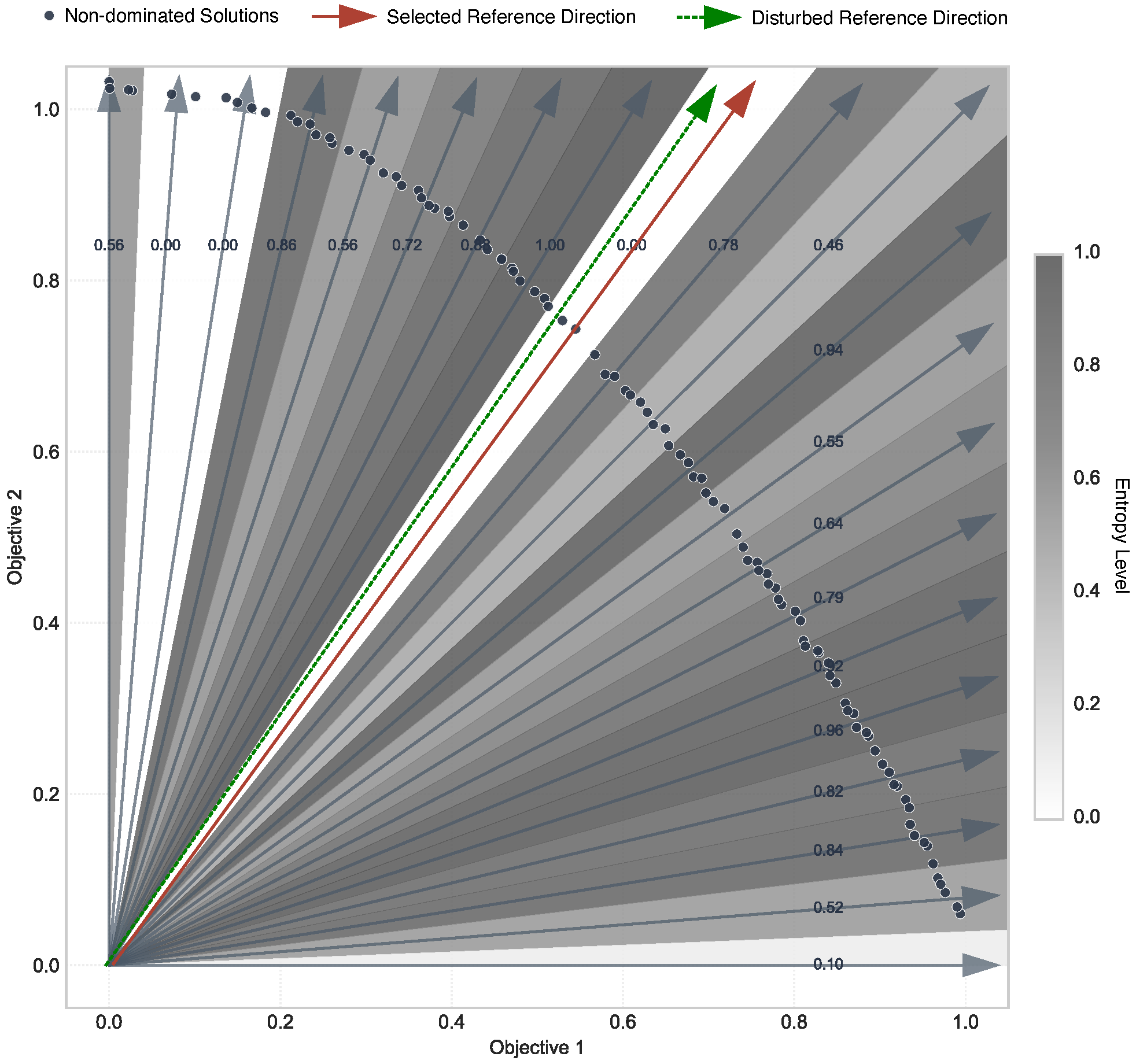
The algorithm begins by initializing key components in lines 1–3, including the external archive $\mathcal{A}$, the ideal point ${\mathbf{z}}^{*}$, the nadir point ${\mathbf{z}}^{nad}$, and the region archive $\mathcal{R}$ based on the provided reference directions. Subsequently, the main loop iteratively executes five key operations. The first step selects the region to be developed based on archive entropy by invoking Algorithm 2. A perturbation is then applied to the reference direction of the selected region through Algorithm 3. This process is further illustrated in Figure 1. Elite solutions within the region are subsequently selected using the Chebyshev scalarization method via Algorithm 4. Neighborhood solutions are generated, and the external archive is updated based on Pareto dominance relations in lines 9–14. With every f iteration, the region archive structure is reconstructed by triggering Algorithm 5. Finally, the algorithm returns a high-quality non-dominated solution set $\mathcal{A}$ in line 19.

It should be supplemented that the objective space is partitioned into N subregions using a pre-defined set of direction vectors $\{{\mathbf{r}}_1,{\mathbf{r}}_2,\dots ,{\mathbf{r}}_N\}$. All individuals in set $\mathcal{A}$ are assigned to these subregions based on the acute angle between their objective vectors and the direction vectors. Each subregion serves as a regional archive, collectively denoted as $\mathcal{R}=\{R_1,R_2,\dots ,R_N\}$. The i-th regional archive $R_i$ is mathematically defined as

$$\begin{array}{c}\hfill R_i=\left\{\mathbf{F}\in {\mathbb{R}}^m|d(\mathbf{F},{\mathbf{r}}_i)\le d(\mathbf{F},{\mathbf{r}}_j),\forall j\ne i\right\}\end{array}$$

where $d(·,·)$ denotes the cosine similarity metric that measures the closeness between a point $\mathbf{F}$ from set $\mathcal{A}$ in the objective space and a direction vector $\mathbf{r}$.

The following subsections provide a detailed description of the five core steps within the main loop of the overall framework.

Algorithm 1: AEG-PLS Framework

Algorithm 2: Select Exploration Region by Archive Entropy

Algorithm 3: Perturb Reference Direction

3.1. Region Exploration Selection by Archive Entropy

To adaptively identify regions with high exploitation potential, this paper proposes an entropy-guided tournament selection mechanism. The procedure is outlined in Algorithm 2.

The process begins at line 1 of Algorithm 2, where the number of candidate regions, $\mathrm{num}=max\left(1,\lfloor (1-s/U)·N\rfloor \right)$, is first determined based on the current iteration. This design encourages a broad search early on and a more focused effort later. Next, line 2 shuffles all region indices randomly. From the first $\mathrm{num}$ of these shuffled candidates, lines 3–10 select the region with the smallest entropy value as the target. Letting $S\left(R\right)$ represent the solution set in region R, its entropy $H\left(R\right)$ is estimated from $S\left(R\right)$. A lower $H\left(R\right)$ indicates a poorer uniformity of solutions within the region in the objective space, signaling higher potential for local exploitation.

Algorithm 4: Select Best Solution by Chebyshev Scalarization

Algorithm 5: Update Region Archive

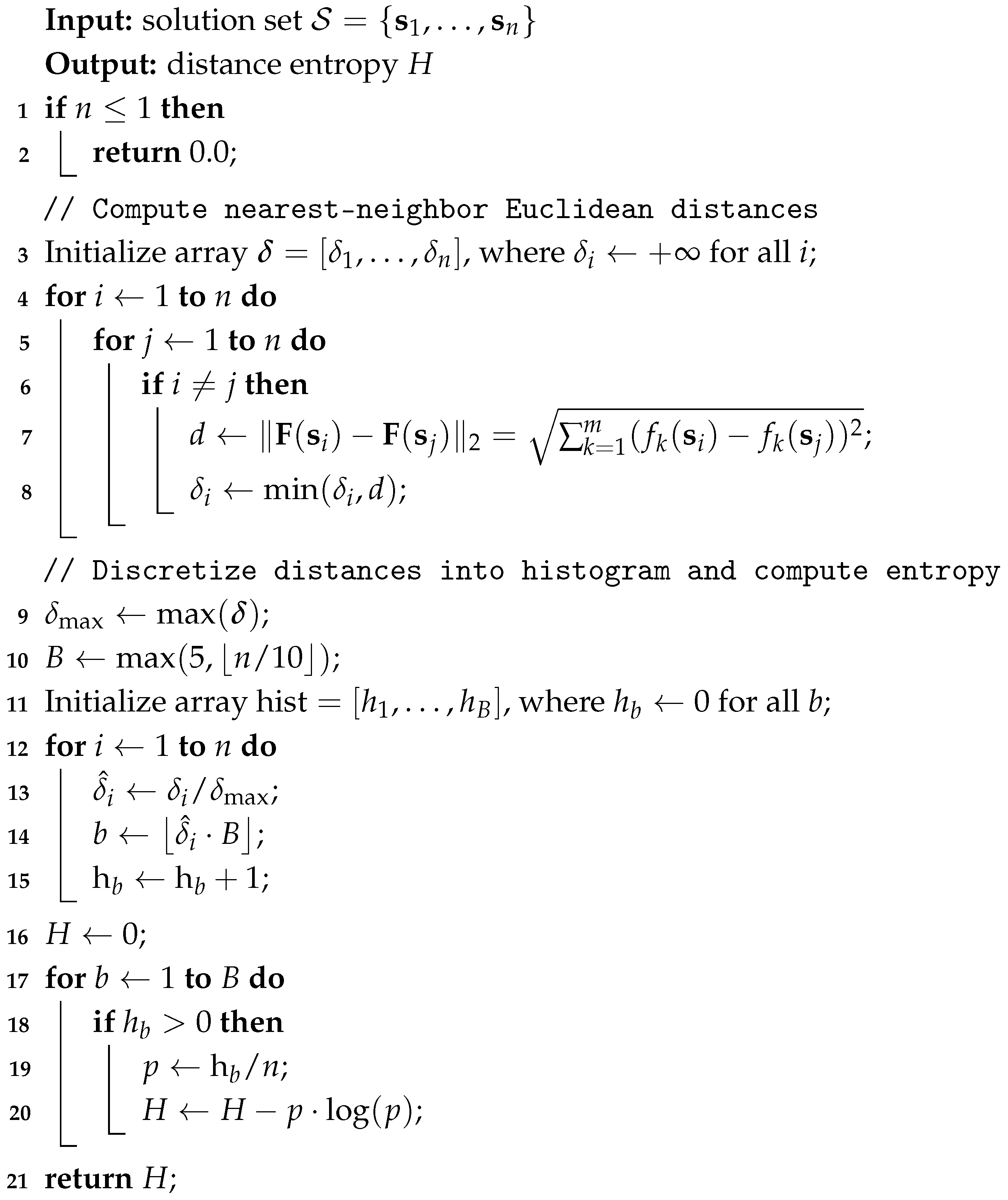
Algorithm 6: Compute Distance Entropy

3.2. Reference Direction Perturbation Mechanism

To enhance the local search capability for complex Pareto fronts, an adaptive perturbation is applied to the reference direction $\mathbf{r}$ of the selected region. The specific procedure is outlined in Algorithm 3. First, a relative Gaussian perturbation $w_j·\mathcal{N}(0,\eta )$ is applied to each weight component $w_j$ of the direction vector (lines 1–4), with the results truncated to the interval $[0,1]$ to ensure the validity of the weights. Here, $\eta ={\displaystyle \frac{1}{N}}{\sum }_{i=1}^N{min}_{\begin{array}{c}j=1,j\ne i\end{array}}^N\parallel {\mathbf{r}}_i-{\mathbf{r}}_j\parallel$, which controls the perturbation strength. Subsequently, the perturbed vector is $L_2$-normalized to yield the new reference direction ${\mathbf{r}}^{\prime }$ (lines 5–7). This strategy introduces controlled adjustments while preserving the original directional characteristics, effectively preventing the search process from converging to local preferences.

3.3. Exploratory Solution Selection Based on Chebyshev Scalarization

Within the selected region $R_{r^{*}}$, the quality of solutions is evaluated using the Chebyshev scalarization method. The specific procedure is outlined in Algorithm 4.

For a region that is non-empty, as defined in line 2, every solution is evaluated by its Chebyshev value, $T\left(\mathbf{x}\right)={max}_i\left\{w_i(f_i\left(\mathbf{x}\right)-z_i^{*})\right\}$, with the process detailed in lines 3–9. The solution yielding the smallest value is selected as the exploratory solution. Conversely, if the region is empty, a solution is randomly chosen from the external archive to allow the search to continue.

3.4. Neighborhood Solutions Generation and External Archive Update

The procedures for neighborhood solution generation and external archive update are described in lines 9–14 of Algorithm 1, which operate as follows.

A neighborhood set $\mathcal{N}$ is first constructed around the elite solution ${\mathbf{x}}^{*}$, as shown in line 9. The definition of this neighborhood is problem-specific; for example, the 2-opt operator can be used for the multi-objective traveling salesman problem (mTSP) [11]. The 2-opt operator is a standard and well-studied neighborhood structure in the mTSP domain, which directly corresponds to the permutation-based encoding and efficiently explores the solution space. Each new solution ${\mathbf{x}}^{\prime }$ is then evaluated in line 12. If it is non-dominated within the external archive, all archive solutions $\mathcal{D}$ dominated by ${\mathbf{x}}^{\prime }$ are removed (lines 13–14), and ${\mathbf{x}}^{\prime }$ itself is added to the archive. Finally, the ideal and nadir points are updated in line 15.

3.5. Region Archive Update and Entropy Estimation

The regional archive structure is reconstructed periodically by invoking Algorithm 5 every f iterations. The existing regional archives are first cleared, as described in lines 1–2. Each solution in the external archive is then normalized and assigned to its most appropriate region according to the cosine distance from the reference directions, with this assignment process covered in lines 5–13. The distance entropy value for each region is subsequently calculated by calling the Algorithm 6, as indicated in line 15 of Algorithm 5.

The computation of distance entropy is described in Algorithm 6. By constructing a histogram of the nearest-neighbor distances among solutions and computing the Shannon entropy based on this distribution, the method effectively quantifies the diversity level within each region.

4. Experiments and Results

4.1. Test Instances

To validate the performance of the proposed algorithm, the mTSP is adopted as a benchmark problem. The mTSP extends the classical Traveling Salesman Problem to scenarios where multiple criteria, such as total travel distance and overall cost, must be optimized simultaneously.

Formally, the mTSP considers a set of n cities and m cost types. For a tour permutation $\pi$ and for each objective $k(k=1,2,\dots ,m)$, the cost function $y_k\left(\pi \right)$ is given by

$$\begin{array}{c}\hfill y_k\left(\pi \right)=\sum _{i=1}^{n-1}{c}_k(v_{\pi \left(i\right)},v_{\pi (i+1)})+c_k(v_{\pi \left(n\right)},v_{\pi \left(1\right)})\end{array}$$

(1)

where $c_k(v_i,v_j)$ denotes the k-th cost of traveling from city $v_i$ to city $v_j$.

The benchmark instances for the mTSP are constructed by combining single-objective TSP instances obtained from public repositories. Here, we adopt two sets of benchmark instances: the Euclidean instances from TSPLIB provided on the website https://eden.dei.uc.pt/~paquete/tsp (accessed on 13 January 2026) and those generated using the DIMACS code. Specifically, we construct 20 test instances by forming all pairwise and triple-wise combinations from the datasets kroA100 through kroE100. Additionally, we include kroAB150, kroAB200, and the DIMACS-generated instances euclidAB100, euclidCD100, and euclidEF100, resulting in a total of 25 test instances.

4.2. Comparative Algorithms

We compared the proposed AEG-PLS with nine baseline algorithms, including PLS [12], NSGA-II [29], and MPLS [19]. Additionally, we considered three conventional variants of the decomposition-based multi-objective evolutionary algorithm [14], MOEA/D-WS, MOEA/D-PBI, and MOEA/D-ASF, along with their enhanced version, EAG-MOEA/D [28]. We also incorporated MOEA/D-DLS [23], a decomposition-based algorithm integrating dynamic local search specifically for multi-objective combinatorial optimization, and AGE-MOEA-II [35], a modern multi-objective evolutionary algorithm recognized for its high performance. The selected algorithms have demonstrated state-of-the-art performance across various benchmark problems.

4.3. Performance Metrics

Evaluating the solution set of an MOP is more complex than in single-objective optimization, as there is no single criterion for directly judging quality. Typically, comprehensive assessment relies on a set of performance indicators. Among these, the Inverted Generational Distance (IGD) [36] and Hypervolume (HV) [37] are two widely adopted metrics. However, since no single indicator can fully capture all aspects of solution set quality [23], this study employs both IGD and HV to facilitate a more robust analysis from different perspectives.

Given the true Pareto front $P{F}^{*}$ of a multi-objective problem, an approximate Pareto front $PF$ obtained using an algorithm, the IGD metric, is calculated as follows:

$$\begin{array}{c}\hfill \begin{array}{c}\hfill \mathrm{IGD}(PF,P{F}^{*})={\displaystyle \frac{1}{|P{F}^{*}|}}\sum _{\mathbf{v}\in P{F}^{*}}\underset{\mathbf{x}\in PF}{min}d(\mathbf{v},\mathbf{x})\end{array}\end{array}$$

(2)

where $d(\mathbf{v},\mathbf{x})$ denotes the Euclidean distance between points $\mathbf{v}$ and $\mathbf{x}$ in the objective space. A smaller IGD value indicates that the approximate front $PF$ is closer to the true Pareto front $P{F}^{*}$, signifying better performance.

The HV metric measures the volume of the objective space dominated by the solution set $PF$ and bounded by a user-defined reference point $\mathbf{r}$. It is defined as

$$\begin{array}{c}\hfill \begin{array}{c}\hfill \mathrm{HV}(PF,\mathbf{r})=\Lambda \left(\bigcup _{\mathbf{x}\in PF}\left[x_1,r_1\right]\times \left[x_2,r_2\right]\times \cdots \times \left[x_m,r_m\right]\right)\end{array}\end{array}$$

(3)

where $\Lambda$ denotes the Lebesgue measure. A larger HV value implies better overall performance of the solution set, reflecting superior convergence and diversity.

It should be noted that in multi-objective optimization, evaluating solution sets requires a true Pareto front. However, for the combinatorial optimization problem studied in this paper, obtaining the exact Pareto front is computationally prohibitive. Therefore, we adopt the method described in [38] to construct a reference set. Specifically, all non-dominated solutions from multiple independent runs of all algorithms are pooled, and the final non-dominated set extracted from this aggregate serves as a proxy for the true Pareto front.

4.4. Experimental Settings

To ensure a fair comparison, all algorithms start from the same initial solution set, and we design two initialization methods for the experimental comparison of algorithms:

The first is a completely random initialization. Without introducing any prior knowledge, we first generate a random population of 100 individuals (N = 100), where each individual is constructed by a random permutation of all cities (i.e., a random Hamiltonian path). Then, the non-dominated solution set is extracted from this population to form the initial external archive ${\mathcal{A}}_0$. Although the initial solutions generated using this method are of poor quality, they provide a fair and unbiased starting point for all algorithms, allowing a direct comparison of their inherent ability to converge to a high-quality Pareto front.

The second is an initialization based on the Lin–Kernighan heuristic [39]. Following the approach used in reference [40], for a multi-objective instance, we randomly select a TSP problem corresponding to one of the objectives and apply the Lin–Kernighan heuristic to generate a high-quality solution. This process is repeated 100 times, and the non-dominated solutions are extracted to construct the initial external archive ${\mathcal{A}}_0$.

All baseline algorithms were configured using the parameter values recommended in their respective original papers. The crossover operator employed Partially Matched Crossover (PMX Crossover) with a crossover probability set to 0.9. The mutation operator utilized Permutation Swap Mutation with a mutation probability of 1.0/n to ensure an average of one mutation per chromosome. Specifically, for non-decomposition-based algorithms, including NSGA-II and AGE-MOEA-II, only the aforementioned basic genetic operator configurations were applied. For decomposition-based MOEA/D algorithms, additional neighborhood search parameters were set: MOEA/D-DLS, MOEA/D-WS, MOEA/D-PBI, and MOEA/D-ASF all adopted a neighborhood size of 20 and a neighborhood selection probability of 0.9, with MOEA/D-DLS executing local search every 100 generations. Among them, as an enhanced algorithm, EAG-MOEA/D employed a distinct neighborhood strategy, with its neighborhood size set to $0.1\times N$ and the neighborhood selection probability set to 1.0.

For the proposed algorithm and other decomposition-based algorithms, the predefined set of direction vectors was generated using the method described in [41], with the number of vectors set to 100. During the local search phase, all algorithms used the 2-opt exchange operator, a standard neighborhood exploration method in the mTSP domain, to explore the neighborhood of selected individuals. The neighborhood depth was uniformly set to 10, and the influence of this parameter will be discussed later in the hyperparameter analysis. The proposed algorithm introduces two additional parameters, the regional archive update frequency and the size limit per regional archive, which were set to 100 and 100, respectively. The sensitivity of these hyperparameters will also be analyzed subsequently.

The execution of each algorithm was terminated upon reaching the maximum number of function evaluations, set at 3000 $\times m\times n$, where m and n represent the number of objectives and the problem size (number of cities), respectively. Each algorithm was independently executed 21 times using distinct random seeds. Furthermore, to obtain a robust overall comparison across all test problems, we applied the Friedman test [42]. This non-parametric method independently ranks the algorithms for each problem and then compares their average rankings. It is particularly suitable for comparing evolutionary optimization algorithms as it does not require assumptions about the distribution of performance data.

The experimental environment consisted of a computer with an 11th Gen Intel® Core™ i7-11700KF processor (16 threads @ 5.0 GHz) under Garuda Linux x86_64. All algorithms were coded in Java using the jMetal framework [43].

4.5. Experimental Results

The performance of the proposed algorithm is evaluated against the baseline algorithms from four aspects, including the mean and standard deviation of performance metrics across multiple runs, an examination of convergence speed through the trajectories of performance metrics, running time comparison, and a comprehensive ranking based on the Friedman test.

4.5.1. Convergence Performance

To clearly present the mean and standard deviation of the performance metrics, this experimental analysis selected MOEA/D-DLS, AGE-MOEA-II, EAG-MOEA/D, MPLS, and the proposed AEG-PLS for comparison. Regarding convergence performance, this experiment conducts an analysis based on two types of initial archives: one generated randomly and the other using the Lin–Kernighan heuristic. The specific results are as follows.

• Random Initialization
  For the test instances derived from TSPLIB,

  Table 1. Performance comparison of algorithms on TSPLIB instances using the IGD metric (with random initialization).

  Test Instances	MOEA/D-DLS	AGE-MOEA-II	EAG-MOEA/D	MPLS	AEG-PLS
  kroAB100	$7.00\times {10}_{1.1\times {10}^{-3}}^{-3}$	$2.36\times {10}_{2.5\times {10}^{-3}}^{-2}$	$5.26\times {10}_{4.7\times {10}^{-4}}^{-3}$	$8.99\times {10}_{1.2\times {10}^{-4}}^{-4}$	$6.70\times {10}_{1.2\times {10}^{-4}}^{-4}$
  kroAC100	$7.62\times {10}_{1.2\times {10}^{-3}}^{-3}$	$2.48\times {10}_{2.4\times {10}^{-3}}^{-2}$	$5.20\times {10}_{6.4\times {10}^{-4}}^{-3}$	$9.00\times {10}_{1.7\times {10}^{-4}}^{-4}$	$6.55\times {10}_{1.5\times {10}^{-4}}^{-4}$
  kroAD100	$7.94\times {10}_{1.5\times {10}^{-3}}^{-3}$	$2.60\times {10}_{3.4\times {10}^{-3}}^{-2}$	$5.85\times {10}_{8.5\times {10}^{-4}}^{-3}$	$8.90\times {10}_{1.4\times {10}^{-4}}^{-4}$	$7.23\times {10}_{1.3\times {10}^{-4}}^{-4}$
  kroAE100	$7.78\times {10}_{1.5\times {10}^{-3}}^{-3}$	$2.65\times {10}_{2.8\times {10}^{-3}}^{-2}$	$5.62\times {10}_{5.9\times {10}^{-4}}^{-3}$	$9.43\times {10}_{1.5\times {10}^{-4}}^{-4}$	$7.18\times {10}_{1.1\times {10}^{-4}}^{-4}$
  kroBC100	$8.24\times {10}_{1.3\times {10}^{-3}}^{-3}$	$2.20\times {10}_{2.6\times {10}^{-3}}^{-2}$	$5.26\times {10}_{6.3\times {10}^{-4}}^{-3}$	$7.35\times {10}_{1.1\times {10}^{-4}}^{-4}$	$6.16\times {10}_{1.2\times {10}^{-4}}^{-4}$
  kroBD100	$5.80\times {10}_{1.2\times {10}^{-3}}^{-3}$	$2.44\times {10}_{2.9\times {10}^{-3}}^{-2}$	$5.02\times {10}_{5.1\times {10}^{-4}}^{-3}$	$8.23\times {10}_{1.3\times {10}^{-4}}^{-4}$	$6.33\times {10}_{1.2\times {10}^{-4}}^{-4}$
  kroBE100	$7.61\times {10}_{1.6\times {10}^{-3}}^{-3}$	$2.24\times {10}_{3.0\times {10}^{-3}}^{-2}$	$4.98\times {10}_{5.4\times {10}^{-4}}^{-3}$	$8.68\times {10}_{1.5\times {10}^{-4}}^{-4}$	$6.67\times {10}_{1.4\times {10}^{-4}}^{-4}$
  kroCD100	$7.85\times {10}_{1.1\times {10}^{-3}}^{-3}$	$2.67\times {10}_{2.9\times {10}^{-3}}^{-2}$	$6.07\times {10}_{7.3\times {10}^{-4}}^{-3}$	$1.01\times {10}_{1.9\times {10}^{-4}}^{-3}$	$8.04\times {10}_{1.8\times {10}^{-4}}^{-4}$
  kroCE100	$7.63\times {10}_{1.4\times {10}^{-3}}^{-3}$	$2.43\times {10}_{3.3\times {10}^{-3}}^{-2}$	$5.26\times {10}_{4.4\times {10}^{-4}}^{-3}$	$8.10\times {10}_{1.4\times {10}^{-4}}^{-4}$	$6.68\times {10}_{1.2\times {10}^{-4}}^{-4}$
  kroDE100	$7.76\times {10}_{1.5\times {10}^{-3}}^{-3}$	$2.21\times {10}_{2.8\times {10}^{-3}}^{-2}$	$5.17\times {10}_{6.6\times {10}^{-4}}^{-3}$	$8.84\times {10}_{1.5\times {10}^{-4}}^{-4}$	$6.77\times {10}_{1.2\times {10}^{-4}}^{-4}$
  kroAB150	$9.51\times {10}_{1.2\times {10}^{-3}}^{-3}$	$2.48\times {10}_{2.5\times {10}^{-3}}^{-2}$	$5.42\times {10}_{5.7\times {10}^{-4}}^{-3}$	$1.24\times {10}_{1.9\times {10}^{-4}}^{-3}$	$9.41\times {10}_{1.6\times {10}^{-4}}^{-4}$
  kroAB200	$9.69\times {10}_{1.1\times {10}^{-3}}^{-3}$	$2.51\times {10}_{2.5\times {10}^{-3}}^{-2}$	$5.15\times {10}_{6.7\times {10}^{-4}}^{-3}$	$1.47\times {10}_{1.4\times {10}^{-4}}^{-3}$	$1.14\times {10}_{1.8\times {10}^{-4}}^{-3}$
  kroABC100	$2.35\times {10}_{1.5\times {10}^{-4}}^{-3}$	$4.21\times {10}_{9.4\times {10}^{-4}}^{-3}$	$1.58\times {10}_{1.4\times {10}^{-4}}^{-3}$	$1.31\times {10}_{1.2\times {10}^{-4}}^{-3}$	$1.23\times {10}_{1.2\times {10}^{-4}}^{-3}$
  kroABD100	$2.30\times {10}_{1.3\times {10}^{-4}}^{-3}$	$4.02\times {10}_{8.8\times {10}^{-4}}^{-3}$	$1.63\times {10}_{1.0\times {10}^{-4}}^{-3}$	$1.28\times {10}_{9.5\times {10}^{-5}}^{-3}$	$1.21\times {10}_{9.5\times {10}^{-5}}^{-3}$
  kroABE100	$2.22\times {10}_{1.8\times {10}^{-4}}^{-3}$	$4.07\times {10}_{9.5\times {10}^{-4}}^{-3}$	$1.69\times {10}_{1.5\times {10}^{-4}}^{-3}$	$1.35\times {10}_{1.3\times {10}^{-4}}^{-3}$	$1.25\times {10}_{9.6\times {10}^{-5}}^{-3}$
  kroACD100	$2.36\times {10}_{2.0\times {10}^{-4}}^{-3}$	$3.87\times {10}_{8.8\times {10}^{-4}}^{-3}$	$1.55\times {10}_{1.5\times {10}^{-4}}^{-3}$	$1.23\times {10}_{1.1\times {10}^{-4}}^{-3}$	$1.19\times {10}_{8.7\times {10}^{-5}}^{-3}$
  kroACE100	$2.67\times {10}_{2.6\times {10}^{-4}}^{-3}$	$4.46\times {10}_{9.3\times {10}^{-4}}^{-3}$	$1.83\times {10}_{1.6\times {10}^{-4}}^{-3}$	$1.40\times {10}_{1.0\times {10}^{-4}}^{-3}$	$1.34\times {10}_{9.5\times {10}^{-5}}^{-3}$
  kroADE100	$2.41\times {10}_{1.4\times {10}^{-4}}^{-3}$	$4.10\times {10}_{7.9\times {10}^{-4}}^{-3}$	$1.76\times {10}_{1.2\times {10}^{-4}}^{-3}$	$1.31\times {10}_{1.0\times {10}^{-4}}^{-3}$	$1.24\times {10}_{9.7\times {10}^{-5}}^{-3}$
  kroBCD100	$2.39\times {10}_{1.9\times {10}^{-4}}^{-3}$	$4.14\times {10}_{8.2\times {10}^{-4}}^{-3}$	$1.76\times {10}_{1.3\times {10}^{-4}}^{-3}$	$1.30\times {10}_{8.3\times {10}^{-5}}^{-3}$	$1.26\times {10}_{8.1\times {10}^{-5}}^{-3}$
  kroBCE100	$2.47\times {10}_{1.6\times {10}^{-4}}^{-3}$	$4.42\times {10}_{7.1\times {10}^{-4}}^{-3}$	$1.83\times {10}_{1.5\times {10}^{-4}}^{-3}$	$1.44\times {10}_{1.3\times {10}^{-4}}^{-3}$	$1.29\times {10}_{1.3\times {10}^{-4}}^{-3}$
  kroBDE100	$2.48\times {10}_{1.7\times {10}^{-4}}^{-3}$	$4.03\times {10}_{7.1\times {10}^{-4}}^{-3}$	$1.56\times {10}_{1.3\times {10}^{-4}}^{-3}$	$1.28\times {10}_{1.7\times {10}^{-4}}^{-3}$	$1.26\times {10}_{1.1\times {10}^{-4}}^{-3}$
  kroCDE100	$2.26\times {10}_{1.4\times {10}^{-4}}^{-3}$	$4.30\times {10}_{7.4\times {10}^{-4}}^{-3}$	$1.67\times {10}_{1.2\times {10}^{-4}}^{-3}$	$1.24\times {10}_{1.0\times {10}^{-4}}^{-3}$	$1.14\times {10}_{8.1\times {10}^{-5}}^{-3}$

  and

  Table 2. Performance comparison of algorithms on TSPLIB instances using the HV metric (with random initialization).

  Test Instances	MOEA/D-DLS	AGE-MOEA-II	EAG-MOEA/D	MPLS	AEG-PLS
  kroAB100	$7.60\times {10}_{1.0\times {10}^{-2}}^{-1}$	$2.34\times {10}_{4.8\times {10}^{-2}}^{-1}$	$7.04\times {10}_{1.2\times {10}^{-2}}^{-1}$	$8.42\times {10}_{3.6\times {10}^{-3}}^{-1}$	$8.48\times {10}_{4.1\times {10}^{-3}}^{-1}$
  kroAC100	$7.35\times {10}_{8.1\times {10}^{-3}}^{-1}$	$2.14\times {10}_{4.2\times {10}^{-2}}^{-1}$	$6.95\times {10}_{2.1\times {10}^{-2}}^{-1}$	$8.24\times {10}_{3.9\times {10}^{-3}}^{-1}$	$8.30\times {10}_{5.4\times {10}^{-3}}^{-1}$
  kroAD100	$7.21\times {10}_{1.1\times {10}^{-2}}^{-1}$	$1.98\times {10}_{5.5\times {10}^{-2}}^{-1}$	$6.65\times {10}_{2.1\times {10}^{-2}}^{-1}$	$8.14\times {10}_{4.5\times {10}^{-3}}^{-1}$	$8.18\times {10}_{3.6\times {10}^{-3}}^{-1}$
  kroAE100	$7.49\times {10}_{8.8\times {10}^{-3}}^{-1}$	$1.88\times {10}_{4.7\times {10}^{-2}}^{-1}$	$6.87\times {10}_{1.6\times {10}^{-2}}^{-1}$	$8.32\times {10}_{5.2\times {10}^{-3}}^{-1}$	$8.37\times {10}_{3.8\times {10}^{-3}}^{-1}$
  kroBC100	$7.67\times {10}_{4.8\times {10}^{-3}}^{-1}$	$2.54\times {10}_{5.2\times {10}^{-2}}^{-1}$	$7.00\times {10}_{1.9\times {10}^{-2}}^{-1}$	$8.49\times {10}_{3.2\times {10}^{-3}}^{-1}$	$8.51\times {10}_{4.3\times {10}^{-3}}^{-1}$
  kroBD100	$7.33\times {10}_{1.1\times {10}^{-2}}^{-1}$	$2.00\times {10}_{5.1\times {10}^{-2}}^{-1}$	$6.75\times {10}_{1.9\times {10}^{-2}}^{-1}$	$8.18\times {10}_{4.6\times {10}^{-3}}^{-1}$	$8.22\times {10}_{3.8\times {10}^{-3}}^{-1}$
  kroBE100	$7.63\times {10}_{6.6\times {10}^{-3}}^{-1}$	$2.68\times {10}_{6.1\times {10}^{-2}}^{-1}$	$7.21\times {10}_{1.2\times {10}^{-2}}^{-1}$	$8.49\times {10}_{5.1\times {10}^{-3}}^{-1}$	$8.53\times {10}_{3.5\times {10}^{-3}}^{-1}$
  kroCD100	$7.49\times {10}_{8.3\times {10}^{-3}}^{-1}$	$2.16\times {10}_{4.9\times {10}^{-2}}^{-1}$	$6.79\times {10}_{2.1\times {10}^{-2}}^{-1}$	$8.36\times {10}_{6.0\times {10}^{-3}}^{-1}$	$8.41\times {10}_{5.6\times {10}^{-3}}^{-1}$
  kroCE100	$7.54\times {10}_{1.5\times {10}^{-2}}^{-1}$	$2.27\times {10}_{5.6\times {10}^{-2}}^{-1}$	$6.94\times {10}_{1.8\times {10}^{-2}}^{-1}$	$8.37\times {10}_{4.5\times {10}^{-3}}^{-1}$	$8.40\times {10}_{3.8\times {10}^{-3}}^{-1}$
  kroDE100	$7.59\times {10}_{1.1\times {10}^{-2}}^{-1}$	$2.63\times {10}_{5.5\times {10}^{-2}}^{-1}$	$7.00\times {10}_{1.8\times {10}^{-2}}^{-1}$	$8.40\times {10}_{4.7\times {10}^{-3}}^{-1}$	$8.45\times {10}_{3.3\times {10}^{-3}}^{-1}$
  kroAB150	$7.12\times {10}_{6.4\times {10}^{-3}}^{-1}$	$1.69\times {10}_{4.4\times {10}^{-2}}^{-1}$	$6.88\times {10}_{1.7\times {10}^{-2}}^{-1}$	$8.04\times {10}_{5.8\times {10}^{-3}}^{-1}$	$8.09\times {10}_{4.5\times {10}^{-3}}^{-1}$
  kroAB200	$6.88\times {10}_{8.8\times {10}^{-3}}^{-1}$	$1.30\times {10}_{3.8\times {10}^{-2}}^{-1}$	$6.89\times {10}_{1.4\times {10}^{-2}}^{-1}$	$7.85\times {10}_{4.5\times {10}^{-3}}^{-1}$	$7.90\times {10}_{6.2\times {10}^{-3}}^{-1}$
  kroABC100	$4.15\times {10}_{1.1\times {10}^{-2}}^{-1}$	$2.21\times {10}_{6.7\times {10}^{-2}}^{-1}$	$4.85\times {10}_{1.5\times {10}^{-2}}^{-1}$	$5.27\times {10}_{1.2\times {10}^{-2}}^{-1}$	$5.28\times {10}_{1.2\times {10}^{-2}}^{-1}$
  kroABD100	$4.22\times {10}_{7.7\times {10}^{-3}}^{-1}$	$2.28\times {10}_{6.3\times {10}^{-2}}^{-1}$	$4.91\times {10}_{1.3\times {10}^{-2}}^{-1}$	$5.31\times {10}_{8.1\times {10}^{-3}}^{-1}$	$5.33\times {10}_{1.1\times {10}^{-2}}^{-1}$
  kroABE100	$4.44\times {10}_{1.2\times {10}^{-2}}^{-1}$	$2.44\times {10}_{6.9\times {10}^{-2}}^{-1}$	$5.01\times {10}_{8.7\times {10}^{-3}}^{-1}$	$5.44\times {10}_{9.0\times {10}^{-3}}^{-1}$	$5.48\times {10}_{9.2\times {10}^{-3}}^{-1}$
  kroACD100	$4.09\times {10}_{1.5\times {10}^{-2}}^{-1}$	$2.29\times {10}_{6.3\times {10}^{-2}}^{-1}$	$4.73\times {10}_{1.9\times {10}^{-2}}^{-1}$	$5.26\times {10}_{1.1\times {10}^{-2}}^{-1}$	$5.26\times {10}_{8.4\times {10}^{-3}}^{-1}$
  kroACE100	$4.07\times {10}_{1.7\times {10}^{-2}}^{-1}$	$2.25\times {10}_{6.2\times {10}^{-2}}^{-1}$	$4.87\times {10}_{1.5\times {10}^{-2}}^{-1}$	$5.29\times {10}_{6.5\times {10}^{-3}}^{-1}$	$5.32\times {10}_{9.8\times {10}^{-3}}^{-1}$
  kroADE100	$4.20\times {10}_{1.0\times {10}^{-2}}^{-1}$	$2.39\times {10}_{5.9\times {10}^{-2}}^{-1}$	$4.89\times {10}_{1.7\times {10}^{-2}}^{-1}$	$5.37\times {10}_{9.2\times {10}^{-3}}^{-1}$	$5.42\times {10}_{1.1\times {10}^{-2}}^{-1}$
  kroBCD100	$4.21\times {10}_{1.3\times {10}^{-2}}^{-1}$	$2.34\times {10}_{6.0\times {10}^{-2}}^{-1}$	$4.86\times {10}_{1.2\times {10}^{-2}}^{-1}$	$5.35\times {10}_{8.9\times {10}^{-3}}^{-1}$	$5.35\times {10}_{9.6\times {10}^{-3}}^{-1}$
  kroBCE100	$4.26\times {10}_{1.0\times {10}^{-2}}^{-1}$	$2.29\times {10}_{4.9\times {10}^{-2}}^{-1}$	$4.88\times {10}_{2.0\times {10}^{-2}}^{-1}$	$5.29\times {10}_{1.1\times {10}^{-2}}^{-1}$	$5.39\times {10}_{9.5\times {10}^{-3}}^{-1}$
  kroBDE100	$4.10\times {10}_{1.2\times {10}^{-2}}^{-1}$	$2.28\times {10}_{5.0\times {10}^{-2}}^{-1}$	$4.85\times {10}_{1.3\times {10}^{-2}}^{-1}$	$5.26\times {10}_{1.3\times {10}^{-2}}^{-1}$	$5.25\times {10}_{9.5\times {10}^{-3}}^{-1}$
  kroCDE100	$4.25\times {10}_{1.2\times {10}^{-2}}^{-1}$	$2.12\times {10}_{4.9\times {10}^{-2}}^{-1}$	$4.87\times {10}_{9.6\times {10}^{-3}}^{-1}$	$5.36\times {10}_{9.6\times {10}^{-3}}^{-1}$	$5.38\times {10}_{1.0\times {10}^{-2}}^{-1}$

  summarize the mean and standard deviation of the IGD and HV metrics, respectively, across 21 independent runs for each algorithm. The best results are highlighted with darker shading. The results in Table 1 show that the proposed AEG-PLS algorithm achieved the best IGD values in all 22 test instances. For HV metrics, Table 2 indicates that AEG-PLS performed optimally in 21 out of the 22 instances, while MPLS achieved the best HV mean on the kroBDE100 instance.

Table 3. Performance comparison of algorithms on DIMACS instances using the IGD metric (with random initialization).

Test Instances	MOEA/D-DLS	AGE-MOEA-II	EAG-MOEA/D	MPLS	AEG-PLS
euclidAB100	$6.98\times {10}_{1.1\times {10}^{-3}}^{-3}$	$8.00\times {10}_{4.8\times {10}^{-4}}^{-3}$	$1.47\times {10}_{8.6\times {10}^{-4}}^{-2}$	$1.29\times {10}_{1.9\times {10}^{-4}}^{-3}$	$1.11\times {10}_{2.1\times {10}^{-4}}^{-3}$
euclidCD100	$8.08\times {10}_{1.3\times {10}^{-3}}^{-3}$	$7.35\times {10}_{5.6\times {10}^{-4}}^{-3}$	$1.38\times {10}_{6.7\times {10}^{-4}}^{-2}$	$1.19\times {10}_{2.0\times {10}^{-4}}^{-3}$	$9.33\times {10}_{1.3\times {10}^{-4}}^{-4}$
euclidEF100	$7.85\times {10}_{1.4\times {10}^{-3}}^{-3}$	$7.62\times {10}_{7.1\times {10}^{-4}}^{-3}$	$1.40\times {10}_{6.4\times {10}^{-4}}^{-2}$	$1.24\times {10}_{1.7\times {10}^{-4}}^{-3}$	$1.06\times {10}_{1.7\times {10}^{-4}}^{-3}$

and

Table 4. Performance comparison of algorithms on DIMACS instances using the HV metric (with random initialization).

Test Instances	MOEA/D-DLS	AGE-MOEA-II	EAG-MOEA/D	MPLS	AEG-PLS
euclidAB100	$7.11\times {10}_{1.1\times {10}^{-2}}^{-1}$	$5.74\times {10}_{1.4\times {10}^{-2}}^{-1}$	$3.95\times {10}_{2.2\times {10}^{-2}}^{-1}$	$7.81\times {10}_{5.6\times {10}^{-3}}^{-1}$	$7.85\times {10}_{6.7\times {10}^{-3}}^{-1}$
euclidCD100	$7.29\times {10}_{9.1\times {10}^{-3}}^{-1}$	$6.11\times {10}_{1.9\times {10}^{-2}}^{-1}$	$4.43\times {10}_{2.5\times {10}^{-2}}^{-1}$	$7.99\times {10}_{5.3\times {10}^{-3}}^{-1}$	$8.03\times {10}_{4.3\times {10}^{-3}}^{-1}$
euclidEF100	$7.42\times {10}_{1.3\times {10}^{-2}}^{-1}$	$6.19\times {10}_{1.9\times {10}^{-2}}^{-1}$	$4.42\times {10}_{2.0\times {10}^{-2}}^{-1}$	$8.07\times {10}_{4.1\times {10}^{-3}}^{-1}$	$8.09\times {10}_{5.6\times {10}^{-3}}^{-1}$

present the mean values and standard deviations of the IGD and HV metrics obtained on the DIMACS test instances, respectively. The results highlighted in gray indicate that AEG-PLS outperforms all compared algorithms in both IGD and HV metrics.

It can be observed that, under the condition of a randomly initialized archive, the proposed AEG-PLS algorithm demonstrates superior and stable performance on the majority of the test instances.

• Lin–Kernighan Heuristic Initialization
  Based on the comparative analysis of performance metrics under the Lin–Kernighan heuristic initialization, the IGD and HV metrics are evaluated on both TSPLIB and DIMACS instances.

  Table 5. Performance comparison of algorithms on TSPLIB instances using the IGD metric (with Lin–Kernighan heuristic initialization).

  Test Instances	MOEA/D-DLS	AGE-MOEA-II	EAG-MOEA/D	MPLS	AEG-PLS
  kroAB100	$1.46\times {10}_{2.9\times {10}^{-4}}^{-3}$	$3.74\times {10}_{4.2\times {10}^{-4}}^{-3}$	$1.11\times {10}_{1.9\times {10}^{-3}}^{-2}$	$6.78\times {10}_{2.1\times {10}^{-4}}^{-4}$	$4.67\times {10}_{1.2\times {10}^{-4}}^{-4}$
  kroAC100	$1.67\times {10}_{2.6\times {10}^{-4}}^{-3}$	$4.02\times {10}_{3.5\times {10}^{-4}}^{-3}$	$1.14\times {10}_{1.2\times {10}^{-3}}^{-2}$	$7.52\times {10}_{1.2\times {10}^{-4}}^{-4}$	$6.41\times {10}_{1.5\times {10}^{-4}}^{-4}$
  kroAD100	$1.93\times {10}_{2.3\times {10}^{-4}}^{-3}$	$3.96\times {10}_{6.5\times {10}^{-4}}^{-3}$	$1.17\times {10}_{2.8\times {10}^{-3}}^{-2}$	$7.56\times {10}_{1.7\times {10}^{-4}}^{-4}$	$5.94\times {10}_{1.6\times {10}^{-4}}^{-4}$
  kroAE100	$1.62\times {10}_{2.9\times {10}^{-4}}^{-3}$	$3.89\times {10}_{6.1\times {10}^{-4}}^{-3}$	$1.12\times {10}_{1.8\times {10}^{-3}}^{-2}$	$6.03\times {10}_{1.9\times {10}^{-4}}^{-4}$	$5.46\times {10}_{1.4\times {10}^{-4}}^{-4}$
  kroBC100	$1.39\times {10}_{3.0\times {10}^{-4}}^{-3}$	$3.31\times {10}_{3.9\times {10}^{-4}}^{-3}$	$9.89\times {10}_{8.2\times {10}^{-4}}^{-3}$	$6.05\times {10}_{1.5\times {10}^{-4}}^{-4}$	$5.16\times {10}_{1.3\times {10}^{-4}}^{-4}$
  kroBD100	$1.44\times {10}_{3.1\times {10}^{-4}}^{-3}$	$3.38\times {10}_{3.8\times {10}^{-4}}^{-3}$	$9.40\times {10}_{1.5\times {10}^{-3}}^{-3}$	$5.66\times {10}_{8.5\times {10}^{-5}}^{-4}$	$4.90\times {10}_{8.4\times {10}^{-5}}^{-4}$
  kroBE100	$1.18\times {10}_{2.2\times {10}^{-4}}^{-3}$	$3.25\times {10}_{3.1\times {10}^{-4}}^{-3}$	$1.00\times {10}_{1.3\times {10}^{-3}}^{-2}$	$6.09\times {10}_{7.5\times {10}^{-5}}^{-4}$	$5.02\times {10}_{1.1\times {10}^{-4}}^{-4}$
  kroCD100	$1.71\times {10}_{5.3\times {10}^{-4}}^{-3}$	$3.89\times {10}_{4.9\times {10}^{-4}}^{-3}$	$1.17\times {10}_{1.4\times {10}^{-3}}^{-2}$	$8.51\times {10}_{1.3\times {10}^{-4}}^{-4}$	$7.03\times {10}_{2.4\times {10}^{-4}}^{-4}$
  kroCE100	$1.75\times {10}_{4.2\times {10}^{-4}}^{-3}$	$3.66\times {10}_{3.8\times {10}^{-4}}^{-3}$	$1.25\times {10}_{1.1\times {10}^{-3}}^{-2}$	$7.47\times {10}_{1.5\times {10}^{-4}}^{-4}$	$6.30\times {10}_{2.1\times {10}^{-4}}^{-4}$
  kroDE100	$1.55\times {10}_{3.8\times {10}^{-4}}^{-3}$	$4.22\times {10}_{2.0\times {10}^{-4}}^{-3}$	$1.17\times {10}_{1.3\times {10}^{-3}}^{-2}$	$9.05\times {10}_{1.1\times {10}^{-4}}^{-4}$	$7.32\times {10}_{1.7\times {10}^{-4}}^{-4}$
  kroAB150	$2.46\times {10}_{3.3\times {10}^{-4}}^{-3}$	$3.75\times {10}_{4.0\times {10}^{-4}}^{-3}$	$1.28\times {10}_{1.6\times {10}^{-3}}^{-2}$	$1.06\times {10}_{1.5\times {10}^{-4}}^{-3}$	$9.13\times {10}_{9.5\times {10}^{-5}}^{-4}$
  kroAB200	$3.52\times {10}_{6.2\times {10}^{-4}}^{-3}$	$3.86\times {10}_{4.2\times {10}^{-4}}^{-3}$	$1.36\times {10}_{8.1\times {10}^{-4}}^{-2}$	$1.48\times {10}_{6.7\times {10}^{-5}}^{-3}$	$1.29\times {10}_{1.1\times {10}^{-4}}^{-3}$
  kroABC100	$1.60\times {10}_{2.3\times {10}^{-4}}^{-3}$	$1.74\times {10}_{1.6\times {10}^{-4}}^{-3}$	$1.96\times {10}_{2.4\times {10}^{-4}}^{-3}$	$1.02\times {10}_{8.8\times {10}^{-5}}^{-3}$	$1.04\times {10}_{8.8\times {10}^{-5}}^{-3}$
  kroABD100	$1.53\times {10}_{1.9\times {10}^{-4}}^{-3}$	$1.59\times {10}_{1.5\times {10}^{-4}}^{-3}$	$1.95\times {10}_{2.1\times {10}^{-4}}^{-3}$	$9.12\times {10}_{6.0\times {10}^{-5}}^{-4}$	$9.11\times {10}_{4.3\times {10}^{-5}}^{-4}$
  kroABE100	$1.46\times {10}_{1.0\times {10}^{-4}}^{-3}$	$1.55\times {10}_{1.1\times {10}^{-4}}^{-3}$	$1.83\times {10}_{2.0\times {10}^{-4}}^{-3}$	$8.98\times {10}_{8.2\times {10}^{-5}}^{-4}$	$9.04\times {10}_{4.1\times {10}^{-5}}^{-4}$
  kroACD100	$1.50\times {10}_{2.0\times {10}^{-4}}^{-3}$	$1.73\times {10}_{1.6\times {10}^{-4}}^{-3}$	$2.02\times {10}_{8.3\times {10}^{-5}}^{-3}$	$9.40\times {10}_{6.2\times {10}^{-5}}^{-4}$	$9.25\times {10}_{5.9\times {10}^{-5}}^{-4}$
  kroACE100	$1.53\times {10}_{2.0\times {10}^{-4}}^{-3}$	$1.74\times {10}_{9.3\times {10}^{-5}}^{-3}$	$2.14\times {10}_{1.9\times {10}^{-4}}^{-3}$	$9.78\times {10}_{1.0\times {10}^{-4}}^{-4}$	$9.63\times {10}_{5.4\times {10}^{-5}}^{-4}$
  kroADE100	$1.70\times {10}_{1.9\times {10}^{-4}}^{-3}$	$1.66\times {10}_{1.4\times {10}^{-4}}^{-3}$	$2.20\times {10}_{2.3\times {10}^{-4}}^{-3}$	$8.71\times {10}_{8.6\times {10}^{-5}}^{-4}$	$8.95\times {10}_{6.8\times {10}^{-5}}^{-4}$
  kroBCD100	$1.59\times {10}_{1.1\times {10}^{-4}}^{-3}$	$1.65\times {10}_{1.2\times {10}^{-4}}^{-3}$	$2.01\times {10}_{1.6\times {10}^{-4}}^{-3}$	$9.65\times {10}_{5.8\times {10}^{-5}}^{-4}$	$9.65\times {10}_{6.3\times {10}^{-5}}^{-4}$
  kroBCE100	$1.60\times {10}_{2.1\times {10}^{-4}}^{-3}$	$1.60\times {10}_{2.0\times {10}^{-4}}^{-3}$	$1.86\times {10}_{1.1\times {10}^{-4}}^{-3}$	$9.52\times {10}_{5.9\times {10}^{-5}}^{-4}$	$9.39\times {10}_{5.1\times {10}^{-5}}^{-4}$
  kroBDE100	$1.51\times {10}_{2.1\times {10}^{-4}}^{-3}$	$1.58\times {10}_{1.6\times {10}^{-4}}^{-3}$	$1.84\times {10}_{1.4\times {10}^{-4}}^{-3}$	$9.21\times {10}_{6.2\times {10}^{-5}}^{-4}$	$9.13\times {10}_{5.4\times {10}^{-5}}^{-4}$
  kroCDE100	$1.53\times {10}_{2.1\times {10}^{-4}}^{-3}$	$1.64\times {10}_{1.4\times {10}^{-4}}^{-3}$	$1.72\times {10}_{1.5\times {10}^{-4}}^{-3}$	$9.73\times {10}_{6.8\times {10}^{-5}}^{-4}$	$9.63\times {10}_{5.4\times {10}^{-5}}^{-4}$

  and

  Table 6. Performance comparison of algorithms on TSPLIB instances using the HV metric (with Lin–Kernighan heuristic initialization).

  Test Instances	MOEA/D-DLS	AGE-MOEA-II	EAG-MOEA/D	MPLS	AEG-PLS
  kroAB100	$8.17\times {10}_{1.2\times {10}^{-2}}^{-1}$	$7.83\times {10}_{8.2\times {10}^{-3}}^{-1}$	$5.95\times {10}_{5.4\times {10}^{-2}}^{-1}$	$8.49\times {10}_{4.8\times {10}^{-3}}^{-1}$	$8.54\times {10}_{3.3\times {10}^{-3}}^{-1}$
  kroAC100	$8.04\times {10}_{1.2\times {10}^{-2}}^{-1}$	$7.77\times {10}_{7.6\times {10}^{-3}}^{-1}$	$5.85\times {10}_{3.4\times {10}^{-2}}^{-1}$	$8.38\times {10}_{3.4\times {10}^{-3}}^{-1}$	$8.41\times {10}_{4.9\times {10}^{-3}}^{-1}$
  kroAD100	$7.76\times {10}_{9.3\times {10}^{-3}}^{-1}$	$7.53\times {10}_{1.2\times {10}^{-2}}^{-1}$	$5.45\times {10}_{8.0\times {10}^{-2}}^{-1}$	$8.20\times {10}_{4.5\times {10}^{-3}}^{-1}$	$8.24\times {10}_{4.3\times {10}^{-3}}^{-1}$
  kroAE100	$8.12\times {10}_{9.3\times {10}^{-3}}^{-1}$	$7.85\times {10}_{1.3\times {10}^{-2}}^{-1}$	$5.94\times {10}_{4.3\times {10}^{-2}}^{-1}$	$8.50\times {10}_{4.4\times {10}^{-3}}^{-1}$	$8.52\times {10}_{3.2\times {10}^{-3}}^{-1}$
  kroBC100	$8.07\times {10}_{1.0\times {10}^{-2}}^{-1}$	$7.87\times {10}_{8.8\times {10}^{-3}}^{-1}$	$6.25\times {10}_{2.1\times {10}^{-2}}^{-1}$	$8.43\times {10}_{3.7\times {10}^{-3}}^{-1}$	$8.45\times {10}_{2.8\times {10}^{-3}}^{-1}$
  kroBD100	$7.99\times {10}_{1.2\times {10}^{-2}}^{-1}$	$7.69\times {10}_{7.6\times {10}^{-3}}^{-1}$	$5.91\times {10}_{4.7\times {10}^{-2}}^{-1}$	$8.33\times {10}_{2.5\times {10}^{-3}}^{-1}$	$8.36\times {10}_{3.3\times {10}^{-3}}^{-1}$
  kroBE100	$8.20\times {10}_{9.6\times {10}^{-3}}^{-1}$	$7.88\times {10}_{7.4\times {10}^{-3}}^{-1}$	$6.10\times {10}_{4.2\times {10}^{-2}}^{-1}$	$8.47\times {10}_{2.1\times {10}^{-3}}^{-1}$	$8.50\times {10}_{3.0\times {10}^{-3}}^{-1}$
  kroCD100	$8.15\times {10}_{1.8\times {10}^{-2}}^{-1}$	$7.92\times {10}_{9.1\times {10}^{-3}}^{-1}$	$5.97\times {10}_{4.3\times {10}^{-2}}^{-1}$	$8.49\times {10}_{2.7\times {10}^{-3}}^{-1}$	$8.54\times {10}_{6.6\times {10}^{-3}}^{-1}$
  kroCE100	$7.98\times {10}_{1.2\times {10}^{-2}}^{-1}$	$7.78\times {10}_{7.6\times {10}^{-3}}^{-1}$	$5.50\times {10}_{3.0\times {10}^{-2}}^{-1}$	$8.36\times {10}_{3.5\times {10}^{-3}}^{-1}$	$8.40\times {10}_{4.2\times {10}^{-3}}^{-1}$
  kroDE100	$8.03\times {10}_{8.3\times {10}^{-3}}^{-1}$	$7.71\times {10}_{5.1\times {10}^{-3}}^{-1}$	$5.75\times {10}_{3.1\times {10}^{-2}}^{-1}$	$8.34\times {10}_{4.4\times {10}^{-3}}^{-1}$	$8.38\times {10}_{2.8\times {10}^{-3}}^{-1}$
  kroAB150	$7.68\times {10}_{1.1\times {10}^{-2}}^{-1}$	$7.71\times {10}_{9.5\times {10}^{-3}}^{-1}$	$5.12\times {10}_{5.5\times {10}^{-2}}^{-1}$	$8.27\times {10}_{2.7\times {10}^{-3}}^{-1}$	$8.30\times {10}_{1.8\times {10}^{-3}}^{-1}$
  kroAB200	$7.21\times {10}_{8.1\times {10}^{-3}}^{-1}$	$7.59\times {10}_{8.9\times {10}^{-3}}^{-1}$	$4.65\times {10}_{3.5\times {10}^{-2}}^{-1}$	$8.06\times {10}_{3.0\times {10}^{-3}}^{-1}$	$8.09\times {10}_{2.7\times {10}^{-3}}^{-1}$
  kroABC100	$4.45\times {10}_{2.3\times {10}^{-2}}^{-1}$	$4.30\times {10}_{1.5\times {10}^{-2}}^{-1}$	$4.32\times {10}_{2.5\times {10}^{-2}}^{-1}$	$5.27\times {10}_{6.9\times {10}^{-3}}^{-1}$	$5.23\times {10}_{5.2\times {10}^{-3}}^{-1}$
  kroABD100	$4.42\times {10}_{1.9\times {10}^{-2}}^{-1}$	$4.34\times {10}_{1.8\times {10}^{-2}}^{-1}$	$4.27\times {10}_{2.5\times {10}^{-2}}^{-1}$	$5.28\times {10}_{8.6\times {10}^{-3}}^{-1}$	$5.30\times {10}_{9.1\times {10}^{-3}}^{-1}$
  kroABE100	$4.73\times {10}_{1.3\times {10}^{-2}}^{-1}$	$4.57\times {10}_{1.3\times {10}^{-2}}^{-1}$	$4.48\times {10}_{2.8\times {10}^{-2}}^{-1}$	$5.55\times {10}_{9.5\times {10}^{-3}}^{-1}$	$5.51\times {10}_{1.1\times {10}^{-2}}^{-1}$
  kroACD100	$4.67\times {10}_{1.7\times {10}^{-2}}^{-1}$	$4.37\times {10}_{1.3\times {10}^{-2}}^{-1}$	$4.30\times {10}_{1.4\times {10}^{-2}}^{-1}$	$5.47\times {10}_{1.2\times {10}^{-2}}^{-1}$	$5.44\times {10}_{7.4\times {10}^{-3}}^{-1}$
  kroACE100	$4.44\times {10}_{2.1\times {10}^{-2}}^{-1}$	$4.23\times {10}_{1.2\times {10}^{-2}}^{-1}$	$4.04\times {10}_{1.8\times {10}^{-2}}^{-1}$	$5.22\times {10}_{9.0\times {10}^{-3}}^{-1}$	$5.24\times {10}_{9.5\times {10}^{-3}}^{-1}$
  kroADE100	$4.13\times {10}_{1.9\times {10}^{-2}}^{-1}$	$4.17\times {10}_{2.0\times {10}^{-2}}^{-1}$	$3.91\times {10}_{1.8\times {10}^{-2}}^{-1}$	$5.17\times {10}_{1.1\times {10}^{-2}}^{-1}$	$5.13\times {10}_{8.3\times {10}^{-3}}^{-1}$
  kroBCD100	$4.64\times {10}_{1.2\times {10}^{-2}}^{-1}$	$4.54\times {10}_{1.6\times {10}^{-2}}^{-1}$	$4.44\times {10}_{2.5\times {10}^{-2}}^{-1}$	$5.47\times {10}_{9.8\times {10}^{-3}}^{-1}$	$5.45\times {10}_{6.8\times {10}^{-3}}^{-1}$
  kroBCE100	$4.57\times {10}_{2.2\times {10}^{-2}}^{-1}$	$4.57\times {10}_{2.5\times {10}^{-2}}^{-1}$	$4.47\times {10}_{1.4\times {10}^{-2}}^{-1}$	$5.43\times {10}_{1.1\times {10}^{-2}}^{-1}$	$5.41\times {10}_{5.9\times {10}^{-3}}^{-1}$
  kroBDE100	$4.52\times {10}_{2.0\times {10}^{-2}}^{-1}$	$4.47\times {10}_{2.1\times {10}^{-2}}^{-1}$	$4.33\times {10}_{1.5\times {10}^{-2}}^{-1}$	$5.37\times {10}_{6.2\times {10}^{-3}}^{-1}$	$5.36\times {10}_{1.1\times {10}^{-2}}^{-1}$
  kroCDE100	$4.65\times {10}_{1.9\times {10}^{-2}}^{-1}$	$4.53\times {10}_{1.9\times {10}^{-2}}^{-1}$	$4.69\times {10}_{2.4\times {10}^{-2}}^{-1}$	$5.43\times {10}_{9.7\times {10}^{-3}}^{-1}$	$5.43\times {10}_{9.7\times {10}^{-3}}^{-1}$

  provide the comparative results for the TSPLIB instances, while

  Table 7. Performance comparison of algorithms on DIMACS instances using the IGD metric (with Lin–Kernighan heuristic initialization).

  Test Instances	MOEA/D-DLS	AGE-MOEA-II	EAG-MOEA/D	MPLS	AEG-PLS
  euclidAB100	$1.88\times {10}_{2.2\times {10}^{-4}}^{-3}$	$3.22\times {10}_{1.8\times {10}^{-4}}^{-3}$	$1.12\times {10}_{7.3\times {10}^{-4}}^{-2}$	$7.14\times {10}_{1.1\times {10}^{-4}}^{-4}$	$5.77\times {10}_{8.6\times {10}^{-5}}^{-4}$
  euclidCD100	$1.73\times {10}_{3.5\times {10}^{-4}}^{-3}$	$3.34\times {10}_{2.0\times {10}^{-4}}^{-3}$	$9.94\times {10}_{9.0\times {10}^{-4}}^{-3}$	$5.74\times {10}_{1.1\times {10}^{-4}}^{-4}$	$4.67\times {10}_{8.0\times {10}^{-5}}^{-4}$
  euclidEF100	$1.85\times {10}_{2.5\times {10}^{-4}}^{-3}$	$3.59\times {10}_{2.5\times {10}^{-4}}^{-3}$	$1.01\times {10}_{8.0\times {10}^{-4}}^{-2}$	$6.62\times {10}_{9.6\times {10}^{-5}}^{-4}$	$5.61\times {10}_{1.0\times {10}^{-4}}^{-4}$

  and

  Table 8. Performance comparison of algorithms on DIMACS instances using the HV metric (with Lin–Kernighan heuristic initialization).

  Test Instances	MOEA/D-DLS	AGE-MOEA-II	EAG-MOEA/D	MPLS	AEG-PLS
  euclidAB100	$7.65\times {10}_{7.4\times {10}^{-3}}^{-1}$	$7.50\times {10}_{4.1\times {10}^{-3}}^{-1}$	$5.25\times {10}_{2.2\times {10}^{-2}}^{-1}$	$8.06\times {10}_{3.4\times {10}^{-3}}^{-1}$	$8.10\times {10}_{2.7\times {10}^{-3}}^{-1}$
  euclidCD100	$7.65\times {10}_{1.2\times {10}^{-2}}^{-1}$	$7.47\times {10}_{5.1\times {10}^{-3}}^{-1}$	$5.61\times {10}_{2.9\times {10}^{-2}}^{-1}$	$8.08\times {10}_{3.0\times {10}^{-3}}^{-1}$	$8.12\times {10}_{1.8\times {10}^{-3}}^{-1}$
  euclidEF100	$7.60\times {10}_{9.6\times {10}^{-3}}^{-1}$	$7.33\times {10}_{6.7\times {10}^{-3}}^{-1}$	$5.39\times {10}_{2.5\times {10}^{-2}}^{-1}$	$8.05\times {10}_{3.3\times {10}^{-3}}^{-1}$	$8.08\times {10}_{3.1\times {10}^{-3}}^{-1}$

  present the corresponding results for the DIMACS instances. In the case of two objectives, Table 5 and Table 6 show that AEG-PLS achieves the best results in both IGD and HV metrics across all test instances from the TSPLIB and DIMACS series. For the three-objective TSPLIB instances, the performance of AEG-PLS is comparable to that of MPLS, yet it still outperforms all other compared algorithms.

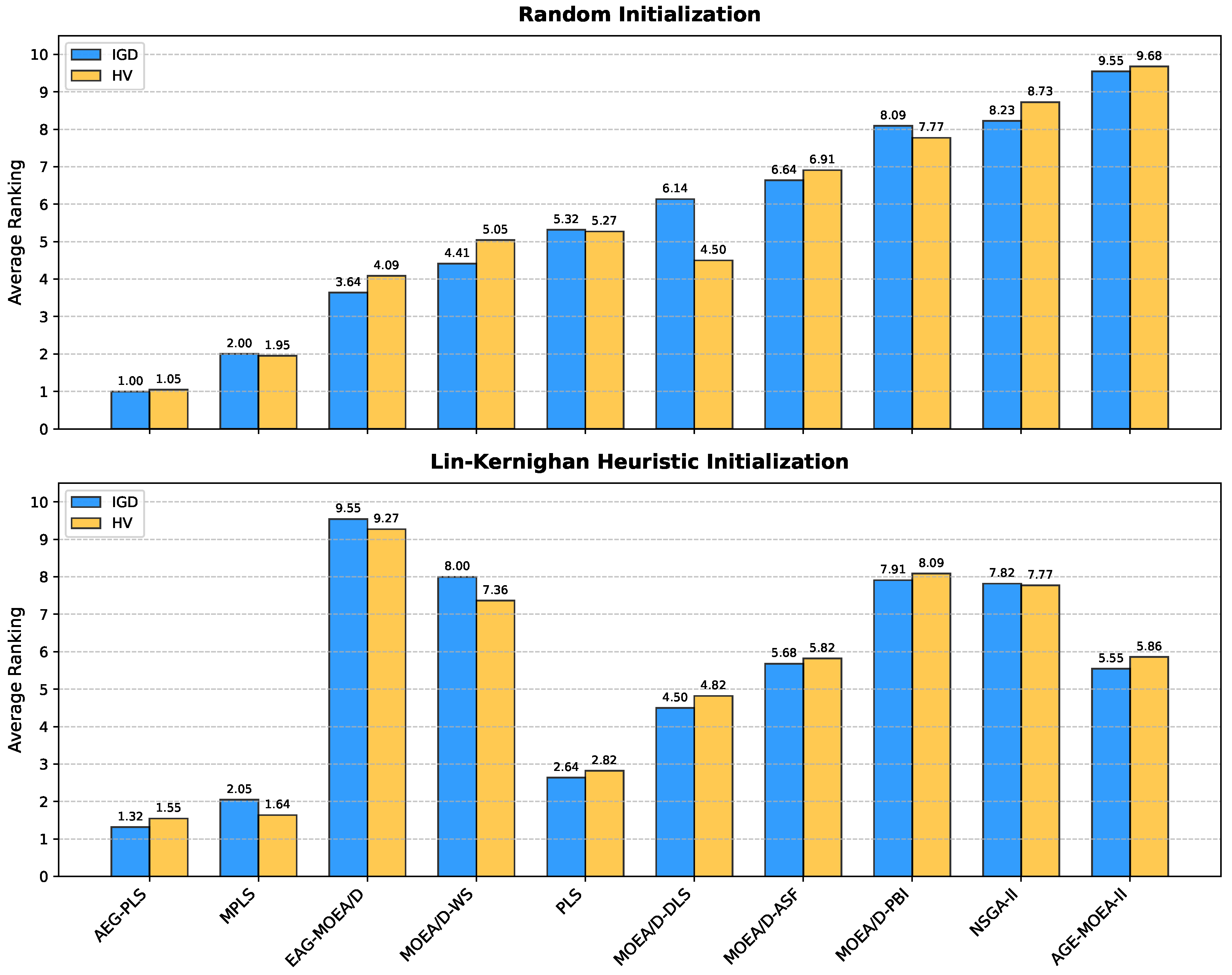
Subsequently, we conducted a comprehensive comparison of algorithm performance using the Friedman test on TSPLIB test instances. The results, depicted in Figure 2, show that our proposed AEG-PLS algorithm achieved the best average rankings on both the IGD and HV metrics, with scores of 1.00 and 1.05, respectively, with random initialization, significantly outperforming all other compared algorithms. And with the Lin–Kernighan heuristic initialization, AEG-PLS also secured the top average rankings of 1.32 and 1.55 for the IGD and HV metrics, respectively. This result provides statistical confirmation of the overall superiority of AEG-PLS in addressing TSPLIB problems.

4.5.2. Convergence Speed Analysis

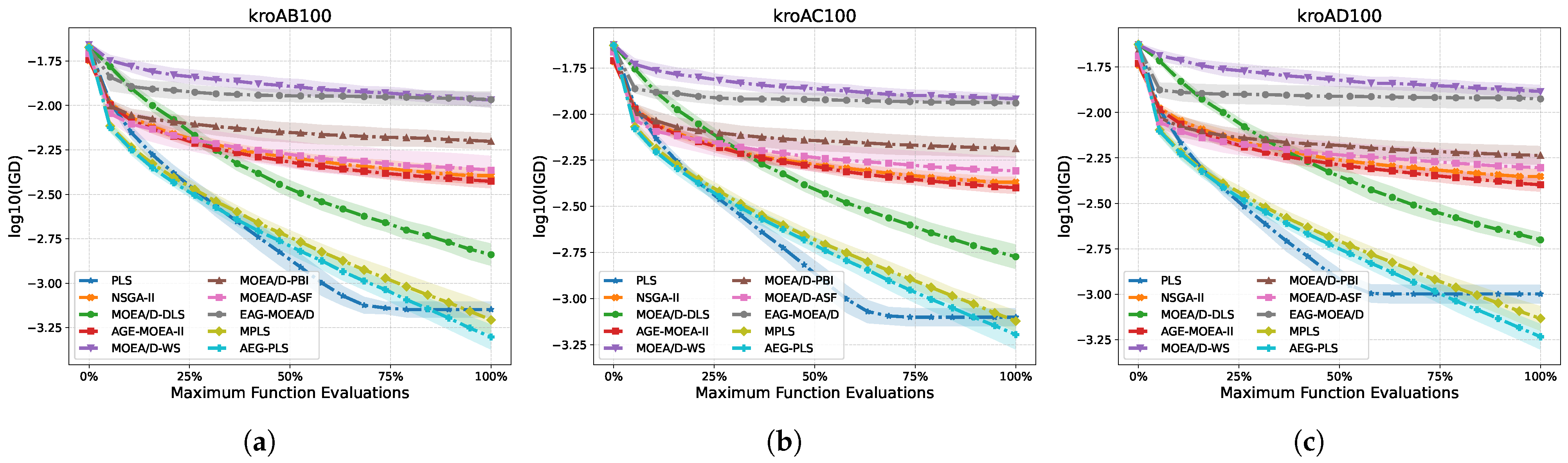
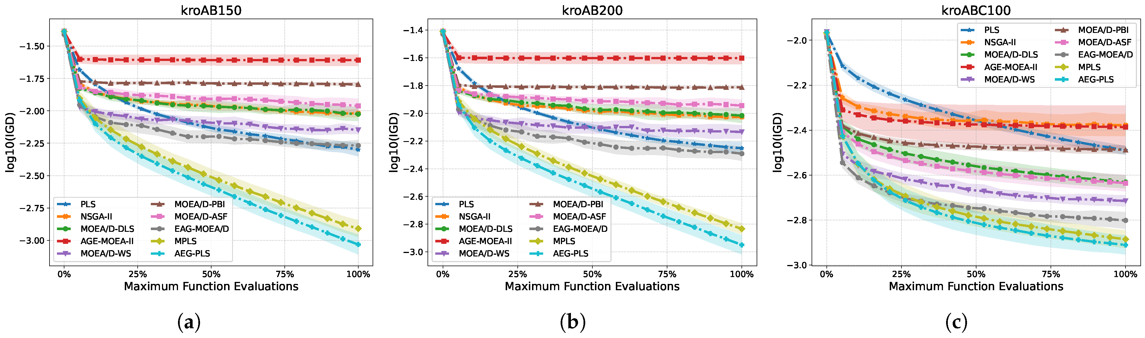
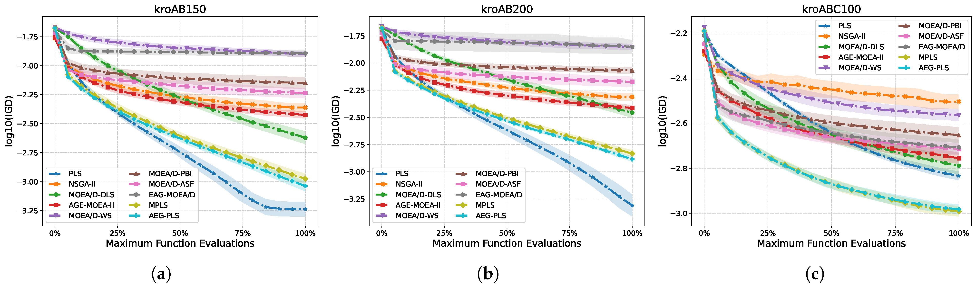
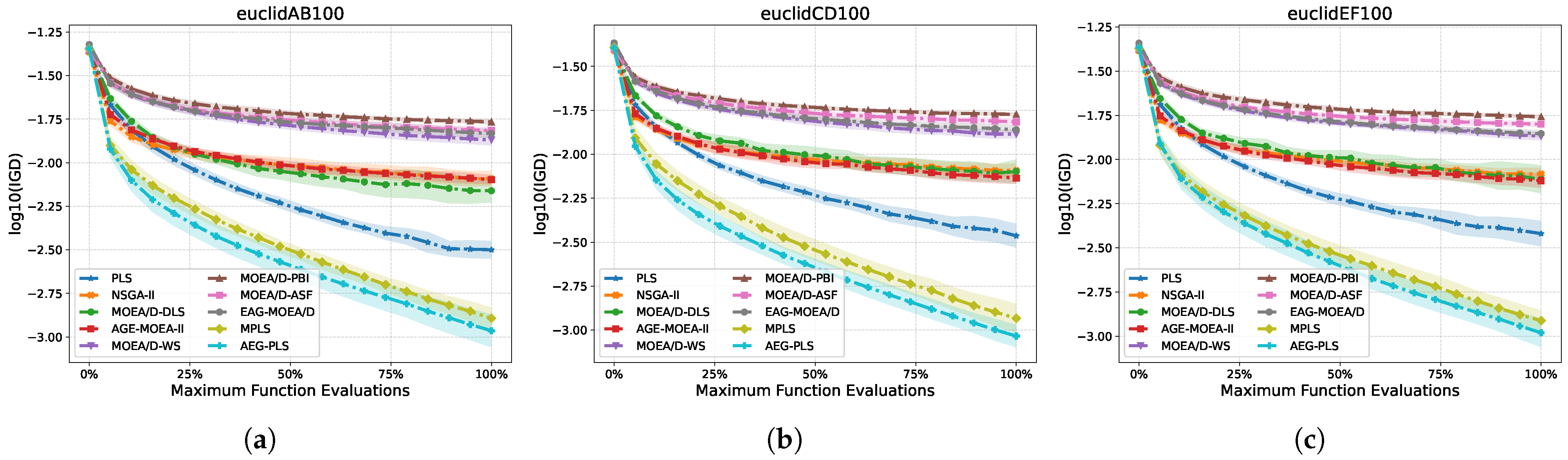
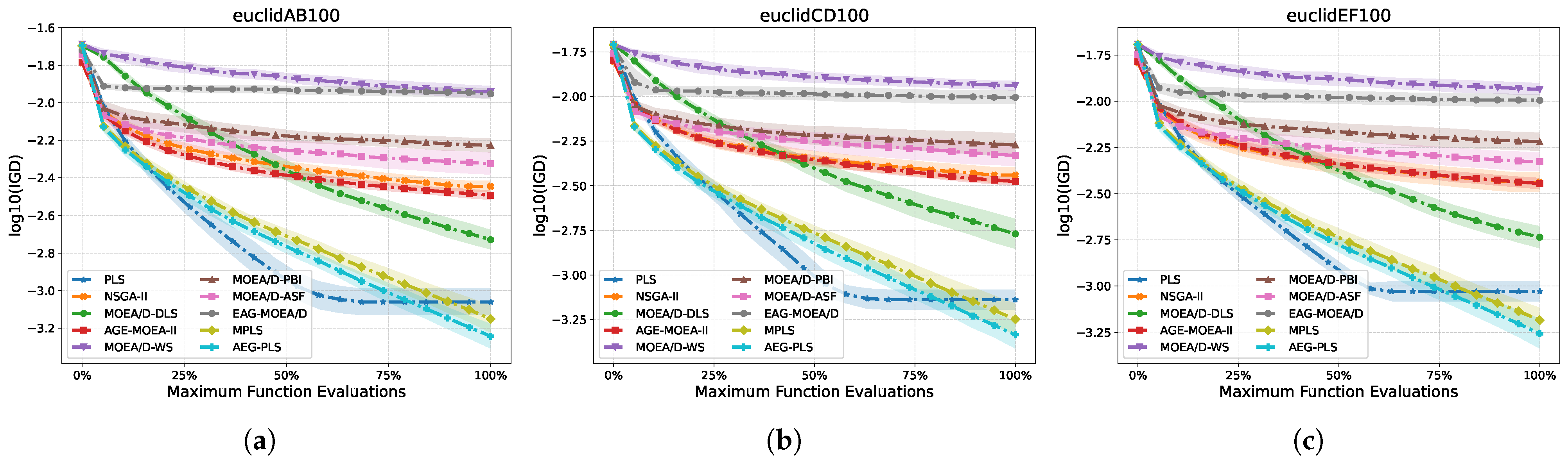
In the comparative analysis of convergence speed, the proposed algorithm is compared with the aforementioned nine algorithms, and their performance is evaluated based on the trends of the mean, best, and worst values of the logarithmic IGD (log10(IGD)) metric.

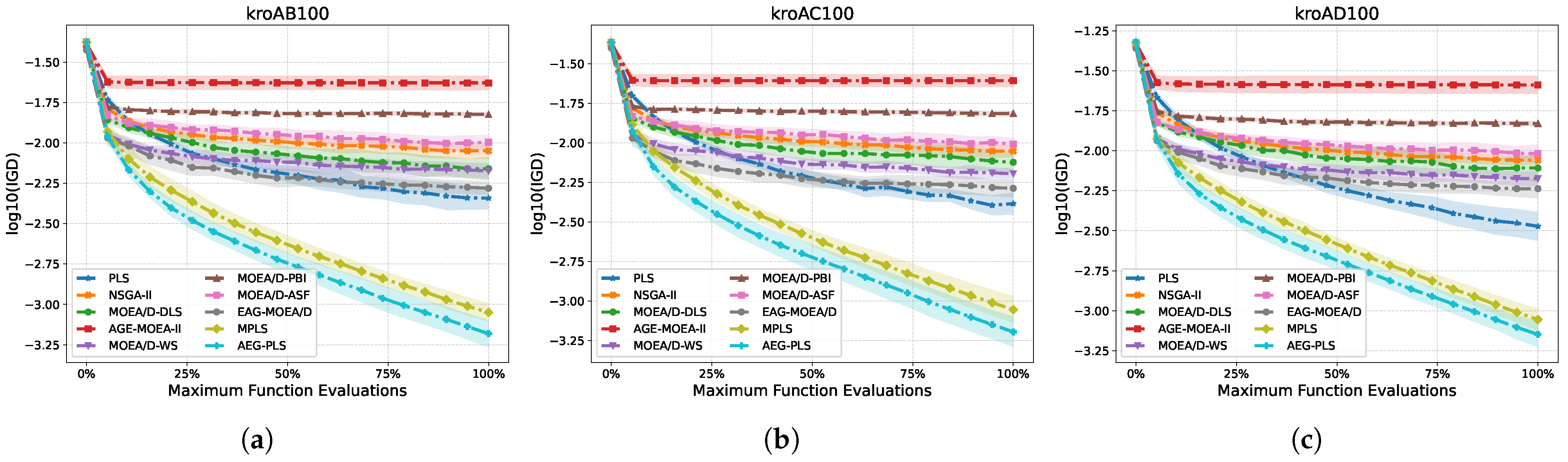
In the experiments, we take the kroAB100, kroAC100, and kroAD100 instances (shown in Figure 3 and Figure 4) and kroAB150, kroAB200, kroABC100 (shown in Figure 5 and Figure 6) from the TSPLIB instances and euclidAB100, euclidCD100, euclidEF100 (shown in Figure 7 and Figure 8) from the DIMACS instances. The convergence processes of all algorithms are illustrated under two initialization schemes: random initialization and initialization via the Lin–Kernighan heuristic. In these figures, the dashed–dotted lines represent the mean values, while the shaded areas indicate the range between the best and worst values.

As can be seen from the figure, under random initialization, AEG-PLS consistently demonstrates a more stable convergence process across all tested instances. Compared to other baseline algorithms, AEG-PLS exhibits a clear advantage in convergence at the early stages of iteration. Although the MPLS algorithm also achieves relatively fast convergence, our proposed AEG-PLS further enhances convergence efficiency by incorporating an entropy-guided Pareto local search strategy. The convergence processes of the algorithms exhibit certain differences when using the Lin–Kernighan heuristic initialization compared to random initialization. It is particularly noteworthy that PLS demonstrates faster convergence in the early stages of algorithm iteration, but as the iteration progresses, its performance no longer improves after exhaustively exploring individuals in the archive. In contrast, our proposed algorithm exhibits stronger resilience, continuously exploring and exploiting under the same termination conditions, thereby achieving ongoing convergence. This also indirectly indicates that PLS is highly sensitive to the initial solution. The primary reason for this is that PLS lacks an effective exploration mechanism, excessively relying on the local exploitation of a few high-quality individuals’ neighborhoods during the search process.

4.5.3. Running Time Comparison

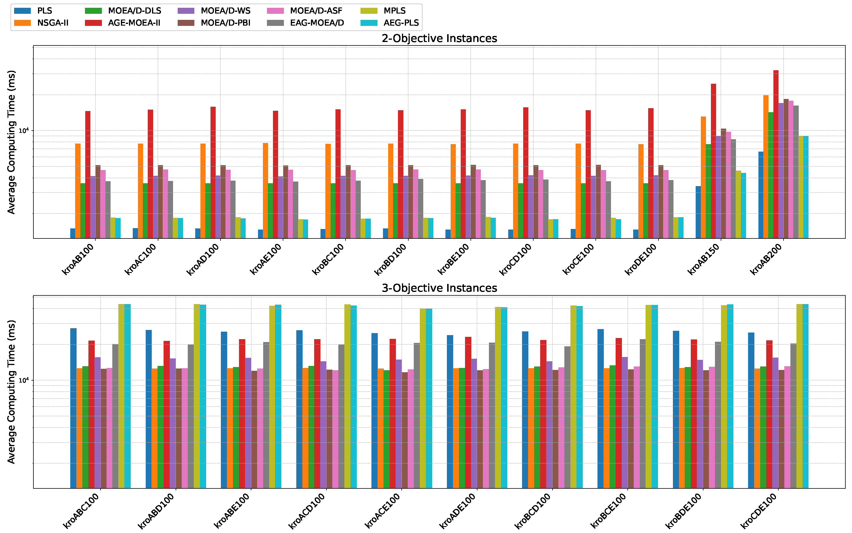
We compared the average running time of each algorithm on the TSPLIB test instances, as shown in Figure 9, and we obtained the following important findings: First, in the case of two objectives, the traditional PLS algorithm had the shortest runtime. The main reason for this lies in its design: once there are no improvable neighboring solutions around the current solution set, the algorithm automatically terminates, even if the preset threshold for the maximum number of objective function evaluations has not been reached. This indirectly indicates that traditional PLS struggles with exploration, easily falls into local optima, and has difficulty maintaining population diversity. In contrast, the proposed AEG-PLS algorithm also performed excellently on two-objective problems, with a runtime second only to that of traditional PLS and better than all other compared algorithms. This is because during the local search process, AEG-PLS generates offspring within selected regions, and its computational cost is generally lower than the crossover and mutation operations commonly used in traditional evolutionary algorithms. This provides AEG-PLS with a certain advantage in time efficiency.

However, as the number of objectives increased to three, the runtime of AEG-PLS increased significantly, even surpassing that of some of the compared algorithms. This is because, in a many-objective environment, the algorithm retains a much larger number of non-dominated solutions in the external archive to maintain better solution set distribution and diversity. This directly leads to an increase in computational burden in two aspects: first, the overhead of updating the external archive and maintaining dominance relationships grows quadratically with the archive size; second, the computational cost of reconstructing the regional archive structure and estimating entropy also increases accordingly. Although these mechanisms help maintain distribution and convergence in many-objective optimization, they also correspondingly increase the overall computational time of the algorithm.

4.6. Parameter Sensitivity Analysis

We conducted a sensitivity analysis on three key parameters of the proposed algorithm: the neighborhood depth of the Pareto local search, the number of regions for objective space partitioning (the number of reference directions), and the update frequency of the regional archive based on the TSPLIB test instances with the random initialization. The Friedman test of the IGD metric was employed to assess the average ranking of the algorithm under different parameter configurations. Our analysis focused first on the individual impact of the local search neighborhood depth, followed by the combined influence of the number of regions and the regional archive update frequency.

4.6.1. Neighborhood Depth

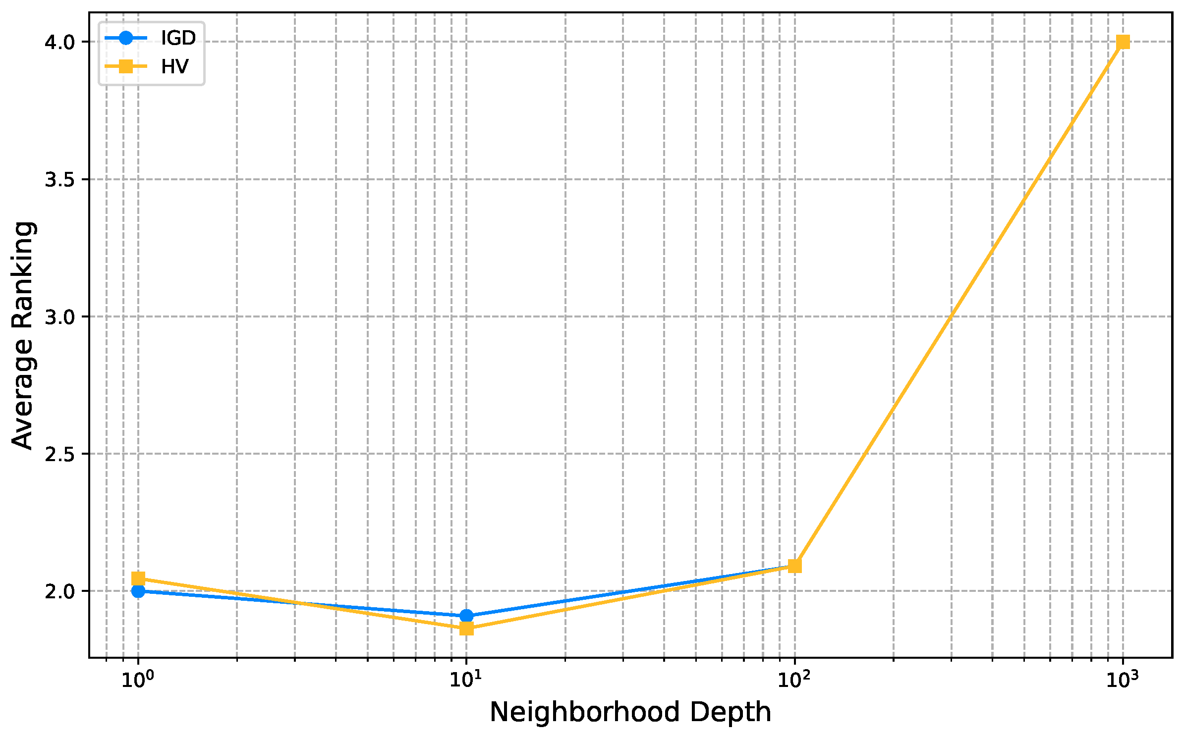
This experiment investigates the impact of the neighborhood depth parameter by testing values from the set {1, 10, 100, 1000}. A depth of 1 signifies that a single neighboring solution is randomly selected via a 2-opt operation for exploration, while a depth of 100 indicates the random selection of 100 neighboring solutions. The experimental results are presented in Figure 10.

The findings indicate that the algorithm achieves a better average ranking when the depth parameter is set to a smaller value, with the most competitive performance observed at a depth of 10. This outcome can be attributed to the fact that a smaller search depth allows the algorithm to utilize computational resources more efficiently during the local search phase. It helps avoid excessive computational overhead caused by evaluating a large number of random neighbors, thereby striking an effective balance between solution quality and search efficiency.

4.6.2. Update Frequency and Number of Regions

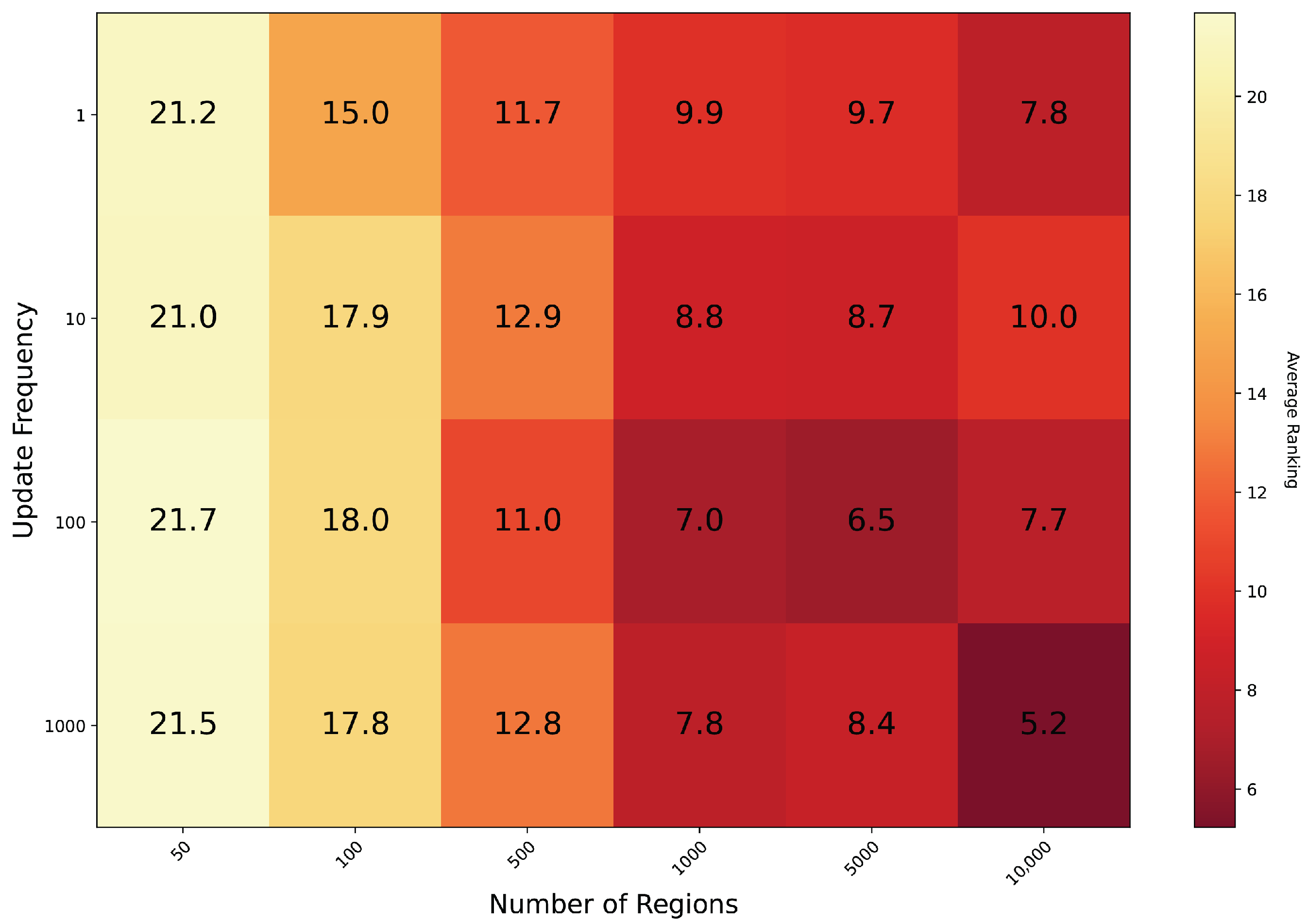
We further analyze the joint influence of the number of regions and the update frequency of the regional archive. The number of regions was tested with values from the set {50, 100, 500, 1000, 5000, 10,000}, while the update frequency was selected from {1, 10, 100, 1000}. Figure 11 presents a heatmap of the Friedman test average rankings corresponding to these parameter combinations. In the heatmap, a darker red color indicates a better average ranking, signifying superior performance, whereas a lighter yellow color corresponds to a worse ranking.

The results indicate that the number of regions has a significant impact on algorithmic performance. Configurations with a larger number of regions generally achieve better overall performance. In contrast, the update frequency exhibits a relatively minor influence. However, completely disabling the update mechanism would prevent the algorithm from dynamically capturing the distribution changes within each regional archive. Conversely, an excessively high number of regions, while beneficial for performance, substantially increases computational complexity. To strike a balance between performance and computational efficiency, both parameters were set to 100 in the comparative experiments presented in the previous section. This configuration, corresponding to a mid-range value for the number of regions, yielded competitively strong performance without excessive computational cost.

5. Conclusions and Future Work

This paper has proposed a novel archive entropy-guided Pareto local search algorithm, termed AEG-PLS, for multi-objective combinatorial optimization. The key idea is to leverage an archive entropy measure to dynamically guide the search process. Specifically, the objective space is partitioned into subregions using a set of reference vectors, and the entropy of each subregion is computed to reflect its current diversity level. The subregion with the lowest entropy, indicating the most severe lack of diversity, is selected as the promising search direction. A high-quality solution from that region is then used to initiate a Pareto local search. Extensive experiments on a set of benchmark instances demonstrate that AEG-PLS achieves highly competitive performance compared to nine state-of-the-art algorithms in terms of both convergence and diversity.

Nevertheless, the proposed algorithm is not without its limitations. A primary concern is its computational efficiency when the number of objectives increases. The mechanisms for entropy calculation, subregion management, and local search exploration all incur additional overhead that can significantly increase the algorithm’s running time in many-objective optimization scenarios. Additionally, while this study validates the effectiveness of the AEG-PLS framework on classic instances, its performance and generalizability across other types of MCOPs, such as problems with different graph structures, objective correlation patterns, or other benchmark families (e.g., the multi-objective knapsack problem and the quadratic assignment problem), require further investigation.

In future work, we intend to explore more efficient mechanisms for entropy estimation and subregion selection to improve scalability. Extending the evaluation to a broader set of combinatorial problems and instance types, and applying the entropy-guided principle to other optimization frameworks, are also important directions for validating and generalizing the proposed approach.

References

1. Agrawal, A.; Ghune, N.; Prakash, S.; Ramteke, M. Evolutionary algorithm hybridized with local search and intelligent seeding for solving multi-objective Euclidian TSP. Expert Syst. Appl. 2021, 181, 115192. [Google Scholar] [CrossRef] [Scilit]
2. Shao, Y.; Lin, J.C.W.; Srivastava, G.; Guo, D.; Zhang, H.; Yi, H.; Jolfaei, A. Multi-Objective Neural Evolutionary Algorithm for Combinatorial Optimization Problems. IEEE Trans. Neural Netw. Learn. Syst. 2023, 34, 2133–2143. [Google Scholar] [CrossRef] [Scilit] [PubMed]
3. Dong, Z.; Wang, X.; Tang, L. MOEA/D with a self-adaptive weight vector adjustment strategy based on chain segmentation. Inf. Sci. 2020, 521, 209–230. [Google Scholar]
4. Diaz, J.E.; López-Ibáñez, M. Incorporating decision-maker’s preferences into the automatic configuration of bi-objective optimisation algorithms. Eur. J. Oper. Res. 2021, 289, 1209–1222. [Google Scholar] [CrossRef] [Scilit]
5. Miettinen, K. Nonlinear Multiobjective Optimization; Kluwer Academic Publishers: Boston, MA, USA, 1999. [Google Scholar]
6. Wang, X.; Dong, Z.; Tang, L.; Zhang, Q. Multiobjective Multitask Optimization-Neighborhood as a Bridge for Knowledge Transfer. IEEE Trans. Evol. Comput. 2023, 27, 155–169. [Google Scholar] [CrossRef] [Scilit]
7. Wang, X.; Zhang, J.; Tang, L.; Liu, Y. Evolutionary Direction Learning with Multivariate Gaussian Probabilistic Model for Multiobjective Optimization. IEEE Trans. Evol. Comput. 2025, in press. [Google Scholar] [CrossRef] [Scilit]
8. Wang, Z.; Gombolay, M. Learning Scheduling Policies for Multi-Robot Coordination with Graph Attention Networks. IEEE Robot. Autom. Lett. 2020, 5, 4509–4516. [Google Scholar] [CrossRef] [Scilit]
9. Zhang, C.; Song, W.; Cao, Z.; Zhang, J.; Tan, P.S.; Xu, C. Learning to dispatch for job shop scheduling via deep reinforcement learning. In Proceedings of the 34th International Conference on Neural Information Processing Systems, NIPS ’20, Vancouver, BC, Canada, 6–12 December 2020; Curran Associates Inc.: Red Hook, NY, USA, 2020. [Google Scholar]
10. Jozefowiez, N.; Semet, F.; Talbi, E.G. Multi-objective vehicle routing problems. Eur. J. Oper. Res. 2008, 189, 293–309. [Google Scholar] [CrossRef] [Scilit]
11. Arnold, F.; Sörensen, K. Knowledge-guided local search for the vehicle routing problem. Comput. Oper. Res. 2019, 105, 32–46. [Google Scholar] [CrossRef] [Scilit]
12. Paquete, L.; Chiarandini, M.; Stützle, T. Pareto Local Optimum Sets in the Biobjective Traveling Salesman Problem: An Experimental Study. In Metaheuristics for Multiobjective Optimisation; Gandibleux, X., Sevaux, M., Sörensen, K., T’kindt, V., Eds.; Springer: Berlin/Heidelberg, Germany, 2004; pp. 177–199. [Google Scholar]
13. Shannon, C.E. A mathematical theory of communication. Bell Syst. Tech. J. 1948, 27, 379–423. [Google Scholar]
14. Zhang, Q.; Li, H. MOEA/D: A Multiobjective Evolutionary Algorithm Based on Decomposition. IEEE Trans. Evol. Comput. 2007, 11, 712–731. [Google Scholar] [CrossRef] [Scilit]
15. Wang, X.; Zhao, Y.; Tang, L.; Yao, X. MOEA/D with Spatial–Temporal Topological Tensor Prediction for Evolutionary Dynamic Multiobjective Optimization. IEEE Trans. Evol. Comput. 2025, 29, 764–778. [Google Scholar] [CrossRef] [Scilit]
16. Shi, J.; Sun, J.; Zhang, Q.; Zhang, H.; Fan, Y. Improving Pareto Local Search Using Cooperative Parallelism Strategies for Multiobjective Combinatorial Optimization. IEEE Trans. Cybern. 2024, 54, 2369–2382. [Google Scholar] [CrossRef] [Scilit]
17. Zhao, Q.; Zhang, L.; Pan, Q.; Cui, K.; Zhao, M.; Tian, F.; Hu, B. An On-Board Executable Pareto-Based Iterated Local Search Algorithm for Embedded Multi-Core Processor Task Scheduling. IEEE Trans. Comput. 2025, 74, 3696–3709. [Google Scholar]
18. Dubois-Lacoste, J.; López-Ibáñez, M.; Stützle, T. Anytime Pareto local search. Eur. J. Oper. Res. 2015, 243, 369–385. [Google Scholar] [CrossRef] [Scilit]
19. Jaszkiewicz, A. Many-Objective Pareto Local Search. Eur. J. Oper. Res. 2018, 271, 1001–1013. [Google Scholar] [CrossRef] [Scilit]
20. Luo, Q.; Wu, G.; Ji, B.; Wang, L.; Suganthan, P.N. Hybrid Multi-Objective Optimization Approach with Pareto Local Search for Collaborative Truck-Drone Routing Problems Considering Flexible Time Windows. IEEE Trans. Intell. Transp. Syst. 2022, 23, 13011–13025. [Google Scholar] [CrossRef] [Scilit]
21. Lust, T.; Teghem, J. Two-phase Pareto local search for the biobjective traveling salesman problem. J. Heuristics 2010, 16, 475–510. [Google Scholar]
22. Dubois-Lacoste, J.; López-Ibáñez, M.; Stützle, T. A hybrid TP+PLS algorithm for bi-objective flow-shop scheduling problems. Comput. Oper. Res. 2011, 38, 1219–1236. [Google Scholar]
23. Dong, Z.; Wang, X.; Tang, L. Color-Coating Scheduling with a Multiobjective Evolutionary Algorithm Based on Decomposition and Dynamic Local Search. IEEE Trans. Autom. Sci. Eng. 2021, 18, 1590–1601. [Google Scholar]
24. Shi, J.; Zhang, Q.; Derbel, B.; Liefooghe, A.; Sun, J. Parallel Pareto Local Search Revisited: First Experimental Results on Bi-Objective UBQP. In Proceedings of the Genetic and Evolutionary Computation Conference, GECCO ’18, Kyoto, Japan, 15–19 July 2018; pp. 753–760. [Google Scholar]
25. Shi, J.; Zhang, Q.; Sun, J. PPLS/D: Parallel Pareto Local Search Based on Decomposition. IEEE Trans. Cybern. 2020, 50, 1060–1071. [Google Scholar] [CrossRef] [Scilit]
26. Cai, X.; Sun, H.; Zhang, Q.; Huang, Y. A Grid Weighted Sum Pareto Local Search for Combinatorial Multi and Many-Objective Optimization. IEEE Trans. Cybern. 2019, 49, 3586–3598. [Google Scholar] [CrossRef] [Scilit] [PubMed]
27. Cai, X.; Xia, C.; Zhang, Q.; Mei, Z.; Hu, H.; Wang, L.; Hu, J. The Collaborative Local Search Based on Dynamic-Constrained Decomposition with Grids for Combinatorial Multiobjective Optimization. IEEE Trans. Cybern. 2021, 51, 2639–2650. [Google Scholar] [CrossRef] [Scilit] [PubMed]
28. Cai, X.; Li, Y.; Fan, Z.; Zhang, Q. An External Archive Guided Multiobjective Evolutionary Algorithm Based on Decomposition for Combinatorial Optimization. IEEE Trans. Evol. Comput. 2015, 19, 508–523. [Google Scholar]
29. Deb, K.; Pratap, A.; Agarwal, S.; Meyarivan, T. A fast and elitist multiobjective genetic algorithm: NSGA-II. IEEE Trans. Evol. Comput. 2002, 6, 182–197. [Google Scholar] [CrossRef] [Scilit]
30. Jaszkiewicz, A.; Zielniewicz, P. Improving the Efficiency of the Distance-Based Hypervolume Estimation Using ND-Tree. IEEE Trans. Evol. Comput. 2025, 29, 726–733. [Google Scholar] [CrossRef] [Scilit]
31. Voudouris, C.; Tsang, E. Guided local search and its application to the traveling salesman problem. Eur. J. Oper. Res. 1999, 113, 469–499. [Google Scholar] [CrossRef] [Scilit]
32. Voudouris, C.; Tsang, E.P.; Alsheddy, A. Guided Local Search. In Handbook of Metaheuristics; Gendreau, M., Potvin, J.Y., Eds.; Springer: Boston, MA, USA, 2010; pp. 321–361. [Google Scholar]
33. Alsheddy, A.; Voudouris, C.; Tsang, E.P.K.; Alhindi, A. Guided Local Search. In Handbook of Heuristics; Martí, R., Pardalos, P.M., Resende, M.G.C., Eds.; Springer International Publishing: Cham, Switzerland, 2018; pp. 261–297. [Google Scholar]
34. Alsheddy, A.; Tsang, E.E.P.K. Guided Pareto Local Search based frameworks for biobjective optimization. In Proceedings of the IEEE Congress on Evolutionary Computation, Barcelona, Spain, 18–23 July 2010; pp. 1–8. [Google Scholar]
35. Panichella, A. An improved Pareto front modeling algorithm for large-scale many-objective optimization. In Proceedings of the Genetic and Evolutionary Computation Conference, GECCO ’22, Boston, MA, USA, 9–13 July 2022; pp. 565–573. [Google Scholar]
36. Schuetze, O.; Equivel, X.; Lara, A.; Coello Coello, C.A. Some Comments on GD and IGD and Relations to the Hausdorff Distance. In Proceedings of the 12th Annual Conference Companion on Genetic and Evolutionary Computation, GECCO ’10, Portland, OR, USA, 7–11 July 2010; pp. 1971–1974. [Google Scholar]
37. Bosman, P.A.N.; Thierens, D. The balance between proximity and diversity in multiobjective evolutionary algorithms. IEEE Trans. Evol. Comput. 2003, 7, 174–188. [Google Scholar] [CrossRef] [Scilit]
38. Cai, X.; Hu, M.; Gong, D.; Guo, Y.-N.; Zhang, Y.; Fan, Z.; Huang, Y. A decomposition-based coevolutionary multiobjective local search for combinatorial multiobjective optimization. Swarm Evol. Comput. 2019, 49, 178–193. [Google Scholar] [CrossRef] [Scilit]
39. Lin, S.; Kernighan, B.W. An Effective Heuristic Algorithm for the Traveling-Salesman Problem. Oper. Res. 1973, 21, 498–516. [Google Scholar] [CrossRef] [Scilit]
40. Paquete, L.; Stützle, T. A Two-Phase Local Search for the Biobjective Traveling Salesman Problem. In Evolutionary Multi-Criterion Optimization; Fonseca, C.M., Fleming, P.J., Zitzler, E., Thiele, L., Deb, K., Eds.; Springer: Berlin/Heidelberg, Germany, 2003; pp. 479–493. [Google Scholar]
41. Blank, J.; Deb, K.; Dhebar, Y.; Bandaru, S.; Seada, H. Generating Well-Spaced Points on a Unit Simplex for Evolutionary Many-Objective Optimization. IEEE Trans. Evol. Comput. 2021, 25, 48–60. [Google Scholar] [CrossRef] [Scilit]
42. Demšar, J. Statistical Comparisons of Classifiers over Multiple Data Sets. J. Mach. Learn. Res. 2006, 7, 1–30. [Google Scholar]
43. Durillo, J.J.; Nebro, A.J. jMetal: A Java framework for multi-objective optimization. Adv. Eng. Softw. 2011, 42, 760–771. [Google Scholar] [CrossRef] [Scilit]
Figure 1. Schematic of the archive entropy-guided region selection and direction perturbation process. Non-dominated solutions (black dots) are distributed in the objective space. The background color gradient indicates the entropy level of different regions, with darker shades corresponding to higher entropy and lighter shades to lower entropy. The algorithm first selects a region typically characterized by lower entropy and its corresponding reference direction (solid red arrow). A perturbation is then applied to this direction, resulting in a new search direction (dashed green arrow) to guide the subsequent local search.
Applsci 16 00964 g001
Figure 2. Average rankings of all algorithms for the TSPLIB test instances based on the Friedman test.
Applsci 16 00964 g002
Figure 3. Convergence speed comparison of the algorithms on the TSPLIB instances with random initialization. (a) kroAB100; (b) kroAC100; (c) kroAD100.
Applsci 16 00964 g003
Figure 4. Convergence speed comparison of the algorithms on the TSPLIB instances with Lin–Kernighan heuristic initialization. (a) kroAB100; (b) kroAC100; (c) kroAD100.
Applsci 16 00964 g004
Figure 5. Convergence speed comparison of the algorithms on the TSPLIB instances with random initialization. (a) kroAB150; (b) kroAB200; (c) kroABC100.
Applsci 16 00964 g005
Figure 6. Convergence speed comparison of the algorithms on the TSPLIB instances with Lin–Kernighan heuristic initialization. (a) kroAB150; (b) kroAB200; (c) kroABC100.
Applsci 16 00964 g006
Figure 7. Convergence speed comparison of the algorithms on the DIMACS instances with random initialization. (a) euclidAB100; (b) euclidCD100; (c) euclidEF100.
Applsci 16 00964 g007
Figure 8. Convergence speed comparison of the algorithms on the DIMACS instances with Lin–Kernighan heuristic initialization. (a) euclidAB100; (b) euclidCD100; (c) euclidEF100.
Applsci 16 00964 g008
Figure 9. Comparative analysis of algorithm running time across the TSPLIB test instances.
Applsci 16 00964 g009
Figure 10. Average ranking of the proposed algorithm with different neighborhood depths.
Applsci 16 00964 g010
Figure 11. Average ranking of the proposed algorithm with different region size and frequency.
Applsci 16 00964 g011