MRMAFusion: A Multi-Scale Restormer and Multi-Dimensional Attention Network for Infrared and Visible Image Fusion

Abstract

Infrared and visible image fusion improves the visual representation of scenes. Current deep learning-based fusion methods typically rely on either convolution operations for local feature extraction or Transformers for global feature extraction, often neglecting the contribution of multi-scale features to fusion performance. To address this limitation, we propose MRMAFusion, a nested connection model that relies on the multi-scale restoration-Transformer (Restormer) and multi-dimensional attention. We construct an encoder–decoder architecture on UNet++ network with multi-scale local and global feature extraction using convolution blocks and Restormer. Restormer can provide global dependency and more comprehensive attention to texture details of the target region along the vertical dimension, compared to extracting features by convolution operations. Along the horizontal dimension, we enhance MRMAFusion’s multi-scale feature extraction and reconstruction capability by incorporating multi-dimensional attention into the encoder’s convolutional blocks. We perform extensive experiments on the public datasets TNO, NIR and RoadScene and compare with other state-of-the-art methods for both objective and subjective evaluation.

1. Introduction

Image fusion [1] is a technique that integrates complementary features from multiple source images of different modalities into a single composite representation, thereby enhancing subsequent computational analysis [2]. Infrared and visible image fusion serves as a representative paradigm within this domain. Visible sensors excel at capturing rich textural details and structural information under adequate illumination; however, their performance degrades substantially under adverse environmental conditions such as rain, fog, or low-light scenarios. In contrast, infrared imaging leverages thermal radiation to effectively distinguish targets from backgrounds regardless of illumination or weather constraints, yet typically suffers from insufficient texture and edge information. By exploiting the complementary characteristics of these two modalities, fusion techniques generate enhanced images that simultaneously preserve thermal saliency and fine-grained details. Such fused outputs not only conform to human visual perception but also benefit various downstream vision tasks, including object detection [3], semantic segmentation [4], and target tracking [5].

Before deep learning revolutionized the image fusion domain, a variety of conventional approaches had been extensively investigated. These methodologies can be broadly classified into several categories: multi-scale transform-based methods [6,7], sparse representation-based approaches [8,9], and saliency-driven techniques [10]. Multi-scale transform methods decompose source images into coefficient representations at different scales using mathematical tools such as Laplacian pyramids or wavelet transforms; the resulting coefficients are then integrated according to predefined rules and subsequently reconstructed via inverse transformation. Sparse representation approaches learn an overcomplete dictionary from training samples and represent source images as linear combinations of sparse coefficients, which are then combined to synthesize the fused output. Saliency-based methods construct decision maps to guide the extraction and integration of perceptually significant regions. Despite achieving reasonable performance, these traditional paradigms face inherent limitations. Specifically, they heavily rely on handcrafted fusion rules and manually designed feature extractors based on prior assumptions, which lack adaptability to the intrinsic characteristics of diverse imaging scenarios. Furthermore, the complexity introduced by elaborate manual design often restricts their generalization capability and practical applicability.

With the rapid advancement of neural network architectures and the substantial growth in computational resources, deep learning-based fusion techniques have emerged as a dominant research paradigm. These approaches leverage neural networks to perform hierarchical feature extraction, integration, and reconstruction, while employing carefully designed loss functions to constrain the optimization process and generate fused images that preserve both salient targets and fine-grained textures. Contemporary deep learning methods for infrared and visible image fusion can be categorized into four principal branches: autoencoder-based architectures [11,12,13,14,15], convolutional neural network-based frameworks [2,16,17,18], generative adversarial network-based schemes [19,20], and Transformer-based models [21,22,23]. Autoencoder-based methods typically train encoder–decoder networks for feature representation and reconstruction while relying on manually crafted fusion strategies, which inherently limits their adaptability due to excessive dependence on prior knowledge. CNN-based approaches enable direct end-to-end learning for feature extraction and fusion but often struggle to consistently guarantee output quality. GAN-based methods employ adversarial training between generator and discriminator to align the fused image distribution with that of source images; however, they frequently suffer from training instability and suboptimal convergence. Transformer-based techniques exploit self-attention mechanisms to capture long-range dependencies and global contextual information; however, they are constrained by substantial computational complexity and memory overhead.

To overcome these limitations, we propose a nested connection architecture integrating multi-scale Restormer and multi-dimensional attention mechanisms for infrared and visible image fusion [24]. Specifically, we adopt a UNet++ encoder–decoder topology [25] to characterize spatial information across varying resolutions and extract hierarchical deep features. Along the encoder downsampling pathway, convolutional modules are combined with multi-scale Restormer blocks [26] for robust feature representation. Furthermore, nested convolutional connections are established at each encoder scale, and three-dimensional attention weights are learned via the SimAM attention mechanism [27]. The fusion strategy incorporates both one-dimensional spatial attention [28] and two-dimensional channel attention [15] for weighted integration. This multi-dimensional attention scheme significantly enhances the network’s capability to extract both salient target information and textural details.

In this paper, our contributions mainly consist of the following three aspects:

• We design an encoder architecture that vertically integrates improved Restormer blocks with convolutional blocks, jointly preserving local details and global dependencies during multi-scale downsampling. It preserves both local and long-range dependency information, reducing detail loss caused by downsampling across different scales.
• We adopt nested connections in both horizontal encoder and decoder, which fully utilize the features output by intermediate convolutional blocks. Additionally, we integrate the SimAm attention within the encoder’s convolutional blocks to train 3D attention weights. It is combined with the fusion strategy of 1D spatial attention and 2D channel attention to form multidimensional attention, which improves network fusion performance.
• We conducted extensive experiments on the TNO, RoadScene and NIR public datasets. Our proposed method outperforms 10 representative deep learning image fusion methods on both subjective and objective measures.

The rest of the paper is organised in the following way. Section 2 presents background information on deep learning-based image fusion algorithms, Transformer and attention mechanisms. Section 3 details our proposed multidimensional attention model, relying on Restormers and nested connections. In Section 4, we validate the advantages of our model through ablation experiments and comparison tests. Section 5 gives our conclusions.

2. Related Work

This section provides a comprehensive overview of the current research landscape in deep learning-based image fusion algorithms, followed by an in-depth discussion of related advances in Transformer architectures and attention mechanisms.

2.1. Deep Learning-Based Image Fusion

The continuous evolution of deep learning techniques has catalyzed the proliferation of learning-based approaches in the image fusion domain. Li et al. introduced DenseFuse [11], an encoder–decoder framework incorporating dense connectivity patterns alongside a 3 × 3 L1-norm fusion strategy. Building upon this, the same group subsequently developed NestFuse [12], which leverages nested connections to capture multi-scale feature representations and integrates spatial-channel attention within the fusion module. To circumvent the constraints imposed by handcrafted fusion rules, Li further proposed RFN-Net [13], a two-stage encoding architecture grounded in residual learning that employs learnable loss functions to autonomously acquire fusion strategies. Zhao et al. introduced DIDFuse [14] based on the premise that images can be decomposed into base and detail layers; this model trains the encoder–decoder to perform such decomposition through specialized loss constraints, fuses the corresponding components separately, and reconstructs the final output via the decoder. To address the inherent trade-off between local receptive fields and global contextual modeling, Wang et al. presented UNFusion [15], which combines diverse Lp-norm formulations with multi-scale encoder–decoder topologies for comprehensive feature extraction and image reconstruction.

Convolutional neural networks have been extensively adopted in image fusion owing to their superior feature representation capabilities. Zhang et al. proposed IFCNN [2], a pioneering supervised framework trained end-to-end on multi-focus datasets utilizing element-wise averaging for fusion, representing the first general-purpose deep learning solution for image fusion. Recognizing that preserving the balance between intensity and gradient information constitutes a fundamental challenge, Zhang et al. subsequently introduced PMGI [16], which employs gradient-intensity loss to maintain textural fidelity and pixel-intensity loss to preserve histogram characteristics. Xu et al. emphasized the significance of image quality metrics and information entropy in fusion performance, leading to the development of U2Fusion [18], which utilizes VGG-16 for feature extraction and adaptively weights loss components according to quality measurements.

Ma et al. pioneered the application of generative adversarial networks to image fusion through FusionGAN [19], wherein the discriminator ensures that the statistical distribution of fused outputs approximates that of source images. To mitigate the modal imbalance arising from single-discriminator configurations, Ma et al. further proposed DDcGAN [20], which engages one generator in adversarial competition against dual discriminators. These discriminators, respectively, enforce the preservation of thermal target saliency and visible textural details [24] in the synthesized images. This dual-path cascaded architecture substantially enhances texture–target integration, demonstrating marked improvements over prior GAN-based fusion frameworks. In this work, we design an encoder–decoder architecture based on the UNet++ topology that performs progressive downsampling and upsampling operations to comprehensively extract feature information across multiple scales. Additionally, nested skip connections are incorporated at each encoder stage to mitigate information degradation induced by network depth.

2.2. Transformer-Based Fusion Methods

Since its introduction in 2017 [29], the Transformer architecture has demonstrated remarkable capabilities through its self-attention mechanism and parallelizable training paradigm, enabling comprehensive modeling of global contextual dependencies. To mitigate the quadratic computational complexity inherent in standard global attention, Swin-Transformer [30] partitions input images into non-overlapping patches and restricts attention computation within local windows. Ma et al. [21] proposed a hybrid framework that first extracts shallow features via convolutional layers, then facilitates cross-modal feature interaction through Swin-Transformer blocks. Wang et al. [22] developed an adaptive weighting scheme to integrate global representations extracted from hierarchical Swin-Transformer layers. Tang et al. introduced DATFuse [23], a dual-attention residual architecture tailored for infrared and visible image fusion [31]. This approach concatenates convolutional modules with Swin-Transformer blocks for feature extraction and formulates multiple loss terms to guide model optimization, thereby transcending the constraints of manually engineered fusion strategies. Furthermore, TCIGFusion [32] combines Restormer blocks with dynamic large kernel convolutions in a two-stage framework, while TSDGFusion [33] leverages text–semantic dual guidance to improve fusion quality and downstream task performance.

In our proposed method, we design Restormer blocks leveraging global self-attention, which are integrated with convolutional modules through element-wise addition during the downsampling phase to compensate for contextual dependency degradation induced by the UNet++ architecture. Furthermore, within the feed-forward network of each Restormer block, we introduce parallel convolutional branches with four distinct kernel sizes. The channel dimension is equally partitioned into four groups for parallel convolution prior to self-attention computation, substantially enhancing the model’s capacity for vertical multi-scale feature extraction.

2.3. Multi-Dimensional Attention Mechanisms

Attention mechanisms [34] enable neural networks to selectively emphasize informative regions while suppressing irrelevant responses. Beyond the self-attention paradigm employed in Transformers, prevalent attention formulations primarily encompass channel attention, spatial attention, and their hybrid variants. Channel attention computes importance weights across feature channels through aggregation operations, capturing inter-channel correlations to enhance feature discriminability and model performance. Spatial attention alternatively learns position-wise importance within each channel, directing focus toward salient spatial locations. CBAM [35] sequentially cascades channel and spatial attention modules, refining both dimensional representations through pooling and sigmoid activation functions, achieving notable performance gains.

Attention mechanisms have been extensively explored in the image fusion community. Li et al. introduced AttentionFGAN [36], which leverages multi-scale pooling operations to derive attention maps at varying resolutions, thereby strengthening feature extraction and reconstruction capabilities. Tang et al. [37] proposed cross-scale attention for infrared–visible fusion, employing encoder–decoder networks to reconstruct images at multiple resolutions while preserving modality-specific salient information through adversarial training. Liu developed the Attention-guided Wavelet-constrained GAN (AWFGAN) [38], which synergistically combines spatial attention with wavelet decomposition to effectively retain high-frequency target information from both infrared and visible modalities.

Channel attention and spatial attention [39] are conventionally regarded as one-dimensional and two-dimensional attention paradigms, respectively. Existing fusion methods typically employ simple concatenation or parallel deployment of these two mechanisms, which proves insufficient for comprehensive multi-dimensional visual feature extraction and reconstruction. To address this limitation, we incorporate SimAM, a three-dimensional attention module, into the convolutional feature extraction blocks at each encoder scale during training. SimAM operates as a parameter-free attention mechanism grounded in energy function optimization, capable of deriving effective three-dimensional attention weights to boost overall performance.

3. Method

In this Section, our model architecture is presented in Section 3.1. The fusion strategy is then detailed in Section 3.2. Lastly, the loss function details are discussed in Section 3.3.

3.1. Network Architecture

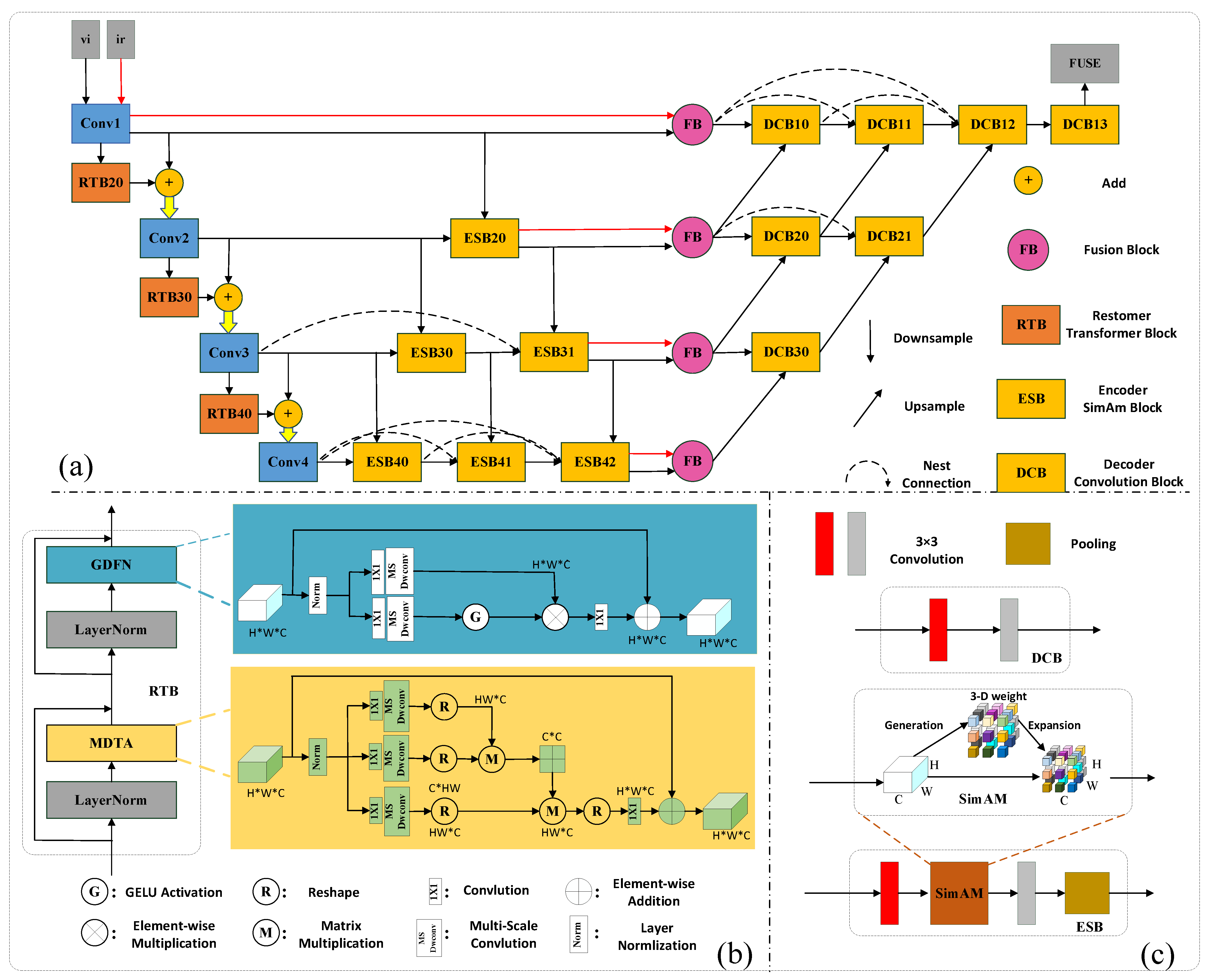
The architecture of our proposed model, illustrated in Figure 1a, consists of three main components: the encoder, the decoder, and the fusion module. The encoder module vertically downsamples infrared and visible images via convolutional operations and uses the improved Restormer to compensate for global dependency information, reducing information loss in the downsampling process. Within each encoder scale, nested convolutional blocks with 3D attention mechanisms efficiently extract image features at the appropriate scales. The decoder utilizes upsampling and nested connections to effectively reconstruct image features, while the fusion module adopts spatial and channel attention weighted fusion of image information.

(1) ESB Module: In this paper, the convolutional blocks in the encoder module are divided into two types: one is the ordinary convolutional block used during downsampling, and the other is the ESB (Encoder SimAM Block) module. The ordinary convolution uses a kernel size of $3\times 3$ with stride set to 2 during downsampling. As shown in Figure 1c, the ESB consists of a $1\times 1$ convolution, a SimAM attention block, and a $3\times 3$ convolution. SimAM is a parameter-free 3D attention mechanism based on energy function optimization. Given an input feature tensor $X\in {\mathbb{R}}^{B\times C\times H\times W}$, where B, C, H, and W denote the batch size, channel number, height, and width, respectively, the attention weight is derived from the inverse energy function:

$$E_i^{-1}={\displaystyle \frac{{(x_i-\mu )}^2}{4({\sigma }^2+\lambda )}}+0.5$$

(1)

where $x_i$ represents each spatial position, $\mu$ and ${\sigma }^2$ are the spatial mean and variance, and $\lambda =0.0001$ is a small constant for numerical stability. The output feature is obtained by $\widehat{X}=X\odot \sigma \left(E^{-1}\right)$, where $\sigma (·)$ denotes the sigmoid function and ⊙ represents element-wise multiplication.

The detailed operation flow of the ESB module is summarized in Algorithm 1.

Table 1. Encoder and decoder network parameter.

	Layer	Input Channel	Output Channel	Resolution	Activation
Encoder	Conv1	1	16	$256\times 256$	ReLU
	Conv2	16	32	$128\times 128$	ReLU
	Conv3	32	48	$64\times 64$	ReLU
	Conv4	48	64	$32\times 32$	ReLU
	RTB20	16	16	$256\times 256$	–
	RTB30	32	32	$128\times 128$	–
	RTB40	48	48	$64\times 64$	–
	ESB20	48	64	$128\times 128$	–
	ESB30	80	96	$64\times 64$	–
	ESB31	208	256	$64\times 64$	–
	ESB40	112	128	$32\times 32$	–
	ESB41	288	304	$32\times 32$	–
	ESB42	752	1024	$32\times 32$	–
Decoder	DCB10	80	16	$256\times 256$	–
	DCB11	96	16	$256\times 256$	–
	DCB12	112	16	$256\times 256$	–
	DCB13	16	1	$256\times 256$	–
	DCB20	320	64	$128\times 128$	–
	DCB21	384	64	$128\times 128$	–
	DCB30	1280	256	$64\times 64$	–

presents the specific parameter settings for all ESB blocks in our network.

Algorithm 1 ESB Module (Encoder SimAM Block)

Require: Input feature $X\in {\mathbb{R}}^{B\times C\times H\times W}$

Ensure: Output feature $\widehat{X}\in {\mathbb{R}}^{B\times C^{\prime }\times H\times W}$   1: $X_1\leftarrow {\mathrm{Conv}}_{1\times 1}\left(X\right)$ {Channel adjustment}   2: // SimAM Attention (parameter-free)   3: $\mu \leftarrow \mathrm{Mean}(X_1,\dim =[H,W])$ {Spatial mean}   4: $d\leftarrow {(X_1-\mu )}^2$ {Squared deviation}   5: $v\leftarrow \mathrm{Mean}(d,\dim =[H,W\left]\right)$ {Variance}   6: $E^{-1}\leftarrow {\displaystyle \frac{d}{4(v+\lambda )}}+0.5$ {Inverse energy, $\lambda =0.0001$}   7: $X_2\leftarrow X_1\odot \sigma \left(E^{-1}\right)$ {Attention weighting}   8: $\widehat{X}\leftarrow {\mathrm{Conv}}_{3\times 3}\left(X_2\right)$ {Feature refinement}   9: return $\widehat{X}$

(2) RTB Module: Considering the loss of global information during convolutional downsampling, we introduce the improved Restormer block to compensate for it through self-attention. As illustrated in Figure 1b, the RTB module consists of two main components, MDTA (Multi-DConv Head Transposed Self-Attention) and GDFN (Gated-Dconv Feed-Forward Network), each preceded by layer normalization.

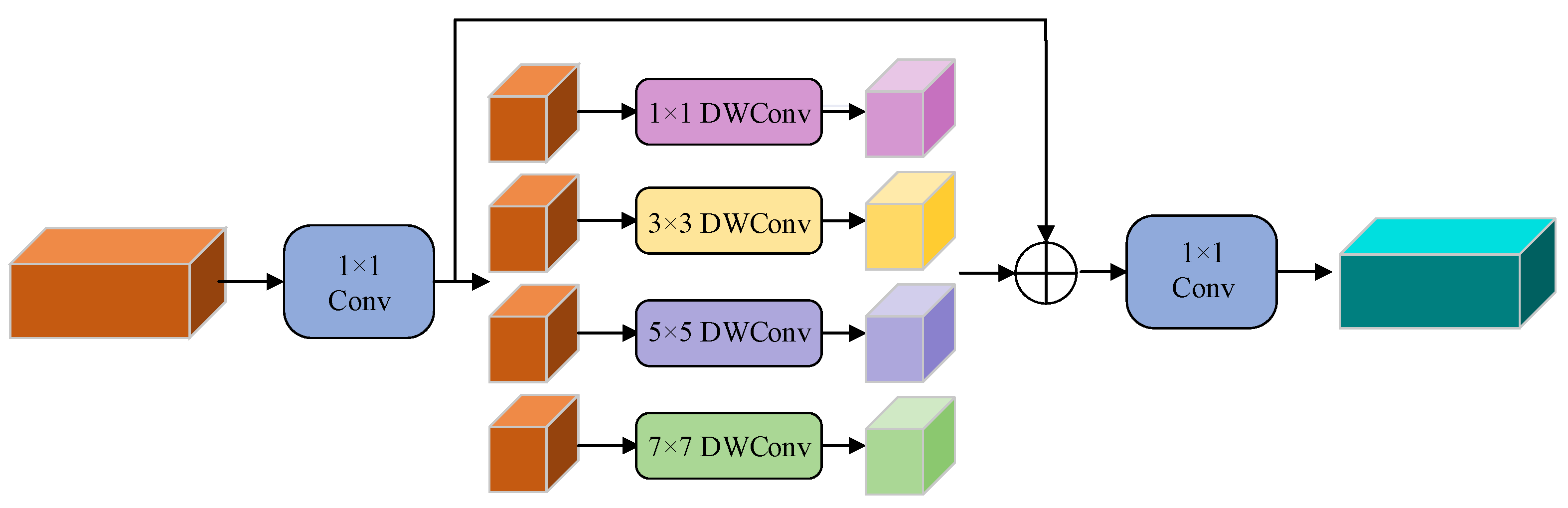
Given an input feature $Y\in {\mathbb{R}}^{H\times W\times C}$, the MDTA module computes transposed self-attention along the channel dimension. After applying layer normalization and $1\times 1$ convolution $W_P$, the feature is split into query Q, key K, and value V, which are then processed by the multi-scale depthwise convolution [40] (Dwconv) operation $W_{MS}$ (illustrated in Figure 2). The $W_{MS}$ operation splits channels into four equal groups and applies depthwise convolutions with kernel sizes of $1\times 1$, $3\times 3$, $5\times 5$, and $7\times 7$ in parallel. The attention mechanism is formulated as follows:

$$Attention(Q,K,V)=V·Softmax(K·Q/\alpha )$$

(2)

$$\tilde{Y}=W_P{W}_{MS}Attention(Q,K,V)+Y$$

(3)

where $Q\in {\mathbb{R}}^{HW\times C}$, $K\in {\mathbb{R}}^{C\times HW}$, $V\in {\mathbb{R}}^{HW\times C}$ are reshaped from the original ${\mathbb{R}}^{H\times W\times C}$ tensors, and $\alpha$ is a learnable scaling parameter.

The GDFN module employs a gating mechanism with the GELU activation function $\varphi (·)$:

$$Gating\left(Y\right)=\varphi \left(W_P{W}_{MS}\left(LN\left(Y\right)\right)\right)\odot W_P{W}_{MS}\left(LN\left(Y\right)\right)$$

(4)

$$\tilde{Y}=W_{MS}Gating\left(Y\right)+Y$$

(5)

where $LN(·)$ denotes layer normalization and ⊙ represents element-wise multiplication.

The complete operation flow of the RTB module is presented in Algorithm 2.

Algorithm 2 RTB Module (Restormer Transformer Block)

Require: Input feature $Y\in {\mathbb{R}}^{H\times W\times C}$

Ensure: Output feature $\tilde{Y}\in {\mathbb{R}}^{H\times W\times C}$   1: // MDTA: Multi-DConv Head Transposed Self-Attention   2: $Y_1\leftarrow \mathrm{LN}\left(Y\right)$ {Layer normalization}   3: $Q,K,V\leftarrow \mathrm{Split}\left({\mathrm{Conv}}_{1\times 1}\left(Y_1\right)\right)$ {Generate Q, K, V}   4: $Q,K,V\leftarrow {\mathrm{W}}_{MS}\left(Q\right),{\mathrm{W}}_{MS}\left(K\right),{\mathrm{W}}_{MS}\left(V\right)$ {Multi-scale Dwconv}   5: $Q^{\prime }\leftarrow \mathrm{Reshape}(Q,[HW,C])$ {Reshape for attention}   6: $K^{\prime }\leftarrow \mathrm{Reshape}(K,[C,HW])$   7: $V^{\prime }\leftarrow \mathrm{Reshape}(V,[HW,C])$   8: $A\leftarrow \mathrm{Softmax}(K^{\prime }·Q^{\prime }/\alpha )$ {Attention map, $A\in {\mathbb{R}}^{C\times C}$}   9: $Y_2\leftarrow \mathrm{Reshape}(V^{\prime }·A,[H,W,C])$   10: $Y_3\leftarrow {\mathrm{Conv}}_{1\times 1}\left({\mathrm{W}}_{MS}\left(Y_2\right)\right)+Y$ {Residual connection}   11: // GDFN: Gated-Dconv Feed-Forward Network   12: $Y_4\leftarrow \mathrm{LN}\left(Y_3\right)$   13: $Y_5\leftarrow {\mathrm{W}}_{MS}\left({\mathrm{Conv}}_{1\times 1}\left(Y_4\right)\right)$ {Expand channels}   14: $Y_6\leftarrow \varphi \left(Y_5\right)\odot Y_5$ {Gating with GELU $\varphi$}   15: $\tilde{Y}\leftarrow {\mathrm{Conv}}_{1\times 1}\left({\mathrm{W}}_{MS}\left(Y_6\right)\right)+Y_3$ {Residual connection}   16: return $\tilde{Y}$

(3) DCB Module: The Decoder Convolution Block (DCB) is designed for feature reconstruction in the decoder pathway. As illustrated in Figure 1c, the DCB module consists of two consecutive 3 × 3 convolution layers. The first convolution layer aggregates features from the concatenated multi-scale inputs received through nested connections and upsampling operations, while the second convolution layer further refines the feature representations. In the decoder, multiple DCB blocks (DCB10-DCB13, DCB20-DCB21, DCB30) progressively reconstruct the fused image features at different scales, as detailed in Table 1. The final DCB13 block outputs a single-channel fused image at the original resolution of 256 × 256.

3.2. Fusion Strategy

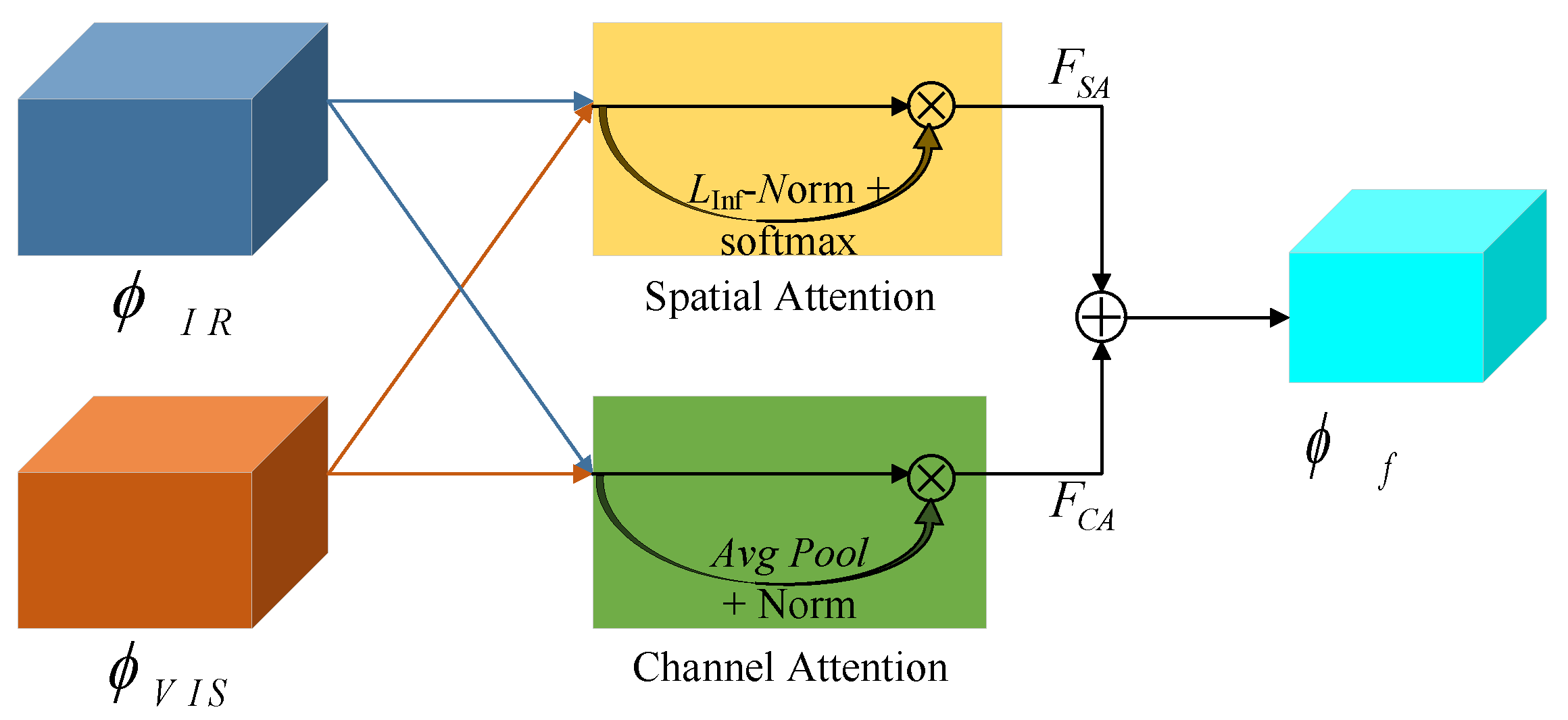
In order to preserve critical input information from both modalities, the fusion module in this work adopts a weighted fusion strategy using both spatial and channel attention. The infrared feature ${\varphi }_{IR}$ and visible feature ${\varphi }_{VIS}$ are jointly processed by the spatial attention module and the channel attention module to generate the respective spatial-based fusion feature $F_{SA}$ and the channel-based fusion feature $F_{CA}$, as illustrated in Figure 3.

To effectively combine these two attention-based features, we design a self-adaptive weighting formula that assigns weights proportional to each feature’s magnitude relative to the total, enabling the fusion module to automatically emphasize the more dominant attention component at each spatial location. When $F_{SA}$ contains stronger responses in texture-rich regions, it receives larger weight; when $F_{CA}$ is more prominent in thermal-salient regions, it contributes more to the final fusion. Compared to simple averaging or learned weights, this parameter-free design provides content-aware fusion without additional learnable parameters, reducing overfitting risk while maintaining adaptive capability. The final fusion feature ${\varphi }_f$ is computed as follows:

$${\varphi }_f=F_{SA}\times {\displaystyle \frac{F_{SA}}{F_{SA}+F_{CA}}}+F_{CA}\times {\displaystyle \frac{F_{CA}}{F_{SA}+F_{CA}}}$$

(6)

As shown in Figure 3, $F_{SA}$ is obtained by multiplying the spatial feature map generated by $L_{Inf}$ Norm and softmax functions with the original feature. Infrared image features ${\varphi }_{IR}$ and visible light image features are ${\varphi }_{VIS}$ both ${\mathbb{R}}^{H\times W\times C}$. The calculated shape of $F_{SA}$ is also ${\mathbb{R}}^{H\times W\times C}$. The process is represented as follows:

$$f_{IR}=\Vert {\varphi }_{IR}{\Vert }_{Inf}$$

(7)

$$f_{VIS}=\Vert {\varphi }_{VIS}{\Vert }_{Inf}$$

(8)

$${\beta }_{IR}^{sa}={\displaystyle \frac{\exp \left(f_{IR}\right)}{\exp \left(f_{IR}\right)+\exp \left(f_{VIS}\right)}}$$

(9)

$${\beta }_{VIS}^{sa}={\displaystyle \frac{\exp \left(f_{VIS}\right)}{\exp \left(f_{IR}\right)+\exp \left(f_{VIS}\right)}}$$

(10)

$$F_{SA}={\varphi }_{IR}\times {\beta }_{IR}^{sa}+{\varphi }_{VIS}\times {\beta }_{VIS}^{sa}$$

(11)

where $\Vert ·{\Vert }_{Inf}$ represents the $L_{Inf}$ Norm calculation, $f_{IR}$ and $f_{VIS}$, respectively, denote the feature maps obtained by $L_{Inf}$ Norm for infrared and visible features, respectively, ${\beta }_{IR}^{sa}$ and ${\beta }_{VIS}^{sa}$ are the spatial weights calculated by weighting.

As shown in Figure 3, $F_{CA}$ is obtained by multiplying the channel feature map generated by global $A\mathrm{vg}P\mathrm{ool}$ and ratio-based normalization with the original feature, and both the input and output shapes are ${\mathbb{R}}^{H\times W\times C}$. The process is represented as follows:

$$f_{IR}=A\mathrm{vg}P\mathrm{ool}({\varphi }_{IR})$$

(12)

$$f_{VIS}=A\mathrm{vg}P\mathrm{ool}({\varphi }_{VIS})$$

(13)

$${\gamma }_{IR}^{ca}={\displaystyle \frac{f_{IR}}{f_{IR}+f_{VIS}}}$$

(14)

$${\gamma }_{VIS}^{ca}={\displaystyle \frac{f_{VIS}}{f_{IR}+f_{VIS}}}$$

(15)

$$F_{CA}={\varphi }_{IR}\times {\gamma }_{IR}^{ca}+{\varphi }_{VIS}\times {\gamma }_{VIS}^{ca}$$

(16)

where $A\mathrm{vg}P\mathrm{ool}$ represents global pooling calculation, ${\gamma }_{IR}^{ca}$ and ${\gamma }_{VIS}^{ca}$ represent the weighted channel values calculated.

3.3. Loss Function

Following the established paradigm in infrared and visible image fusion [11,12,15], we adopt an autoencoder-based training strategy. Since no ground truth exists for fusion tasks, only the encoder and decoder are trained for image self-reconstruction, while the fusion module is excluded. This enables the encoder to learn universal feature representations applicable to both modalities. During testing, infrared and visible images are separately encoded, fused via the attention-based strategy (Section 3.2), and decoded to produce the final result.

To preserve fused image structure and pixel intensity, we adopt $L1$ loss and structural similarity loss, with the specific expression as follows:

$$Loss=L_{L1}+\mu L_{SSIM}$$

(17)

where $\mu$ serves as a hyper-parameter that balances the influence of both loss terms on the model training. In this work, experiments were conducted with $\mu$ taking values of 1, 5, 10, 100, and 1000, and the comparative evaluation of experiment performance is presented in Section 4.

L1 loss is an absolute value loss function which is defined as follows for an image with the same size of input and output dimensions:

$$L_{L1}={\displaystyle \frac{\sum \Vert O-I\Vert }{HW}}$$

(18)

where H and W represent the input image width and height, O and I are fused image and input image.

$SSIM$ is a measure of the brightness, contrast, and structure in the image, ranging from 0 to 1. The higher the value, the more similar the two images are. Therefore, the difference between $SSIM$ and 1 is commonly referred to as loss function $L_{SSIM}$, with the expression as follows:

$$L_{SSIM}=1-SSIM(O,I)$$

(19)

$$SSIM(O,I)={\displaystyle \frac{(2{\mu }_I{\mu }_O+C_1)(2{\sigma }_{IO}+C_2)}{({\mu }_I^2+{\mu }_O^2+C_1)({\sigma }_I^2+{\sigma }_O^2+C_2)}}$$

(20)

where ${\mu }_I$ and ${\mu }_O$ are the average pixel value for the input and output images, the standard deviations are denoted as ${\sigma }_I$ and ${\sigma }_O$, and the correlation coefficient is denoted as ${\sigma }_{IO}$. $C_1$ and $C_2$ are constants to ensure that the denominator is not zero.

4. Experiments

In this section, we introduce our experiment setup and details in Section 4.1, along with relevant image evaluation metrics. We analyze the selection of hyperparameters and perform ablation experiments in Section 4.2. In Section 4.3, we perform qualitative and quantitative comparative experiments and analyses with other fusion methods based on deep learning on the datasets TNO, NIR and RoadScene.

4.1. Experimental Details

We used 80,000 images from the MS-COCO dataset for training. All images were converted to grayscale and resized to $256\times 256$ pixels. The proposed MRMAFusion was implemented in PyTorch 1.8.0 and trained from scratch without any pre-trained weights. We used the Adam optimizer with hyperparameters ${\beta }_1=0.9$ and ${\beta }_2=0.999$, a fixed learning rate of $1\times {10}^{-3}$ without decay scheduling, a batch size of 4, and trained for 4 epochs. No data augmentation was applied during training. All experiments were conducted on an NVIDIA GeForce RTX 4070Ti GPU.

In the test phase, we selected 42 image pairs from TNO, 52 image pairs from NIR and 40 image pairs from RoadScene to evaluate and compare our proposed method. In the comparative experiments of this study, qualitative analysis primarily relies on subjective evaluations by human vision, which can vary significantly among different individuals. Therefore, we introduced quantitative analysis for comparison, employing various formulaic metrics to objectively assess image quality and more fairly evaluate the merits of different methods. We utilized six evaluation metrics, Mutual Information (MI) [41], Entropy (EN) [42], Spatial Frequency (SF) [43], Standard Deviation (SD) [44], Fusion Quality (Qabf) [45], and Visual Information Fidelity (VIF) [46].

4.2. $\mu$ Value Selection and Ablation Experiments

This section presents comparative experiments to select a hyperparameter $\mu$ value in the loss function, and ablation experiments are also performed on the RTB and ESB modules proposed in this paper, demonstrating the superiority of our approach on three datasets.

(1) Selection of the $\mu$ value: The hyperparameter $\mu$ in our loss function (Equation (17)) controls the relative importance between the L1 loss and the SSIM loss. A larger $\mu$ value emphasizes structural similarity preservation, while a smaller value focuses more on pixel-wise intensity consistency. To determine the optimal value, we conducted experiments with $\mu \in \{1,5,10,100,1000\}$, covering a wide range from intensity-dominant to structure-dominant configurations.

As shown in

Table 2. The fusion image metrics with different values of $\mu$ in the three datasets. $\mu$ is the weighting coefficient that balances the L1 loss and SSIM loss in the total loss function (red for best, blue for second best).

Dataset	$\mathit{\mu }$	EN	MI	SF	SD	VIF	Qabf
TNO	1	7.01034	3.68497	9.52341	41.48464	0.87745	0.53287
	5	7.01878	3.73317	10.16536	41.62811	0.89373	0.53723
	10	7.00937	3.65345	10.08234	41.39382	0.87380	0.53041
	100	7.02507	3.64551	9.89553	41.92570	0.87154	0.52993
	1000	7.02071	3.71342	9.67823	41.76024	0.88941	0.53368
NIR	1	7.35249	4.71012	17.24790	49.15533	0.94346	0.60329
	5	7.36145	4.75487	18.55717	49.30941	0.95292	0.60347
	10	7.35683	4.66922	18.57130	49.11026	0.93332	0.59808
	100	7.35312	4.68580	17.89285	49.12542	0.93445	0.59828
	1000	7.35465	4.73748	16.82413	49.09030	0.94849	0.60192
RoadScene	1	7.36990	3.78614	12.78249	49.15461	0.71346	0.50884
	5	7.41757	3.86197	13.99177	50.71819	0.72641	0.50922
	10	7.37889	3.76332	12.78923	49.32286	0.71280	0.50637
	100	7.39970	3.79374	13.87034	50.25727	0.71312	0.50404
	1000	7.39404	3.82886	13.25628	49.99016	0.71900	0.50654

, on the NIR and RoadScene datasets, the evaluation metrics are optimized when $\mu$ is set to 5, while this value also provides the best results for three metrics on the TNO dataset. The value $\mu =5$ achieves a good balance between preserving pixel intensity and maintaining structural similarity. Therefore, we adopt $\mu =5$ for all subsequent experiments.

(2) RTB Module Ablation Experiment: To quantify the contribution of the proposed RTB module compared to plain convolution, we conducted ablation experiments under different configurations during downsampling in the encoder. Specifically, we tested four settings: (1) “Plain Conv (NO-RTB)” where all RTB blocks are replaced with standard convolutional layers, (2) “1-RTB” with only the RTB20 block, (3) “2-RTB” with both RTB20 and RTB30 blocks, and (4) “Ours (3-RTB)” with all three RTB blocks (RTB20, RTB30, and RTB40).

As shown in

Table 3. Ablation study on RTB module: Restormer vs. plain convolution in the three datasets (red for best, blue for second best).

Dataset	Configuration	EN	MI	SF	SD	VIF	Qabf
TNO	Plain Conv (NO-RTB)	7.02100	3.70090	9.45826	41.80793	0.88441	0.53715
	1-RTB	7.02439	3.69958	9.78312	41.96736	0.88294	0.53321
	2-RTB	7.02002	3.70835	10.22783	41.75639	0.88329	0.53317
	Ours (3-RTB)	7.01878	3.73317	10.16536	41.62811	0.89373	0.53723
NIR	Plain Conv (NO-RTB)	7.35783	4.74665	17.12581	49.22418	0.95328	0.60671
	1-RTB	7.35881	4.76207	17.89427	49.30651	0.95231	0.60452
	2-RTB	7.35669	4.72750	18.34712	49.16089	0.95109	0.60420
	Ours (3-RTB)	7.36145	4.75487	18.55717	49.30941	0.95292	0.60347
RoadScene	Plain Conv (NO-RTB)	7.38180	3.81768	12.45813	49.62981	0.72311	0.51772
	1-RTB	7.40297	3.83066	13.23624	50.36707	0.72375	0.51005
	2-RTB	7.37539	3.80123	13.78318	49.35612	0.71946	0.51164
	Ours (3-RTB)	7.41757	3.86197	13.99177	50.71819	0.72641	0.50922

, the “Plain Conv (NO-RTB)” configuration, which uses only standard convolutions without any Restormer blocks, achieves inferior performance in MI and VIF metrics compared to our full model. On the TNO dataset, our method improves MI by 0.87% (from 3.70090 to 3.73317) and VIF by 1.05% (from 0.88441 to 0.89373) compared to plain convolution. Similar improvements are observed on the RoadScene dataset, with MI increasing by 1.16% and VIF by 0.46%. These results demonstrate that the Restormer blocks effectively capture global dependencies through self-attention mechanisms, compensating for the information loss caused by downsampling that plain convolutions cannot address. The progressive improvement with more RTB blocks further validates the effectiveness of our multi-scale Restormer design in preserving salient features and texture details from different modalities.

(3) Multi-dimensional Attention Ablation Experiment: To quantify the contribution of the SimAM 3D attention mechanism, we performed ablation experiments within all ESB blocks of the model. We compared five configurations: (1) “NO-SimAM” where the SimAM attention is completely removed, (2) “CA-Att (1D)” using 1-dimensional channel attention, (3) “SP-Att (2D)” using 2-dimensional spatial attention, (4) “SC-Att” using serial combination of channel and spatial attention, and (5) “SimAM (3D, Ours)” using our proposed 3-dimensional parameter-free attention.

As shown in

Table 4. Different attention fusion image configuration in the three datasets (red for best, blue for second best).

Dataset	Metrics	EN	MI	SF	SD	VIF	Qabf
TNO	NO-simAM	7.00268	3.60090	8.98532	41.20689	0.85804	0.52504
	CA-Att(1D)	7.00477	3.65112	9.34719	41.17492	0.87462	0.53072
	SP-Att(2D)	7.01964	3.70683	9.78295	41.80817	0.88800	0.53379
	SC-Att	7.00651	3.68526	10.05813	41.26345	0.88292	0.53387
	SimAM (3D, Ours)	7.01878	3.73317	10.16536	41.62811	0.89373	0.53723
NIR	NO-simAM	7.35590	4.61427	16.23814	49.05813	0.92143	0.59314
	CA-Att(1D)	7.35818	4.68576	17.12583	49.11274	0.93844	0.59818
	SP-Att(2D)	7.35627	4.75444	18.39205	49.12062	0.95043	0.60229
	SC-Att	7.34832	4.68820	17.89417	47.84280	0.94231	0.60728
	SimAM (3D, Ours)	7.36145	4.75487	18.55717	49.30941	0.95292	0.60347
RoadScene	NO-simAM	7.35847	3.68774	11.56924	48.50586	0.69606	0.50042
	CA-Att(1D)	7.37939	3.76182	12.34853	49.29348	0.71203	0.50494
	SP-Att(2D)	7.41484	3.83969	13.99528	50.03931	0.72135	0.50848
	SC-Att	7.39128	3.80355	13.62984	49.77502	0.71542	0.50424
	SimAM (3D, Ours)	7.41757	3.86197	13.99177	50.71819	0.72641	0.50922

, the “NO-SimAM” configuration achieves the lowest performance across most metrics, demonstrating that removing the SimAM attention significantly degrades the feature extraction capability. On the TNO dataset, compared to the NO-SimAM baseline, our SimAM (3D) improves MI by 3.67% (from 3.60090 to 3.73317) and VIF by 4.16% (from 0.85804 to 0.89373). On the RoadScene dataset, SimAM achieves improvements of 4.73% in MI and 4.36% in VIF over the no-attention baseline.

Furthermore, comparing different attention dimensions, we observe that 2D spatial attention (SP-Att) outperforms 1D channel attention (CA-Att), indicating that spatial information plays a more important role in image fusion. However, our 3D SimAM attention achieves the best overall performance by jointly considering channel, height, and width dimensions through energy function optimization. The serial combination of channel and spatial attention (SC-Att) does not outperform SimAM, suggesting that simply concatenating 1D and 2D attention is less effective than our unified 3D attention approach. These results validate the efficacy of the SimAM mechanism in enhancing multi-dimensional feature extraction and reconstruction for image fusion.

(4) Multi-scale vs. Single-scale Dwconv Ablation Experiment: To evaluate the contribution of multi-scale depthwise convolution in the RTB module, we compare our multi-scale design (with kernel sizes $1\times 1$, $3\times 3$, $5\times 5$, and $7\times 7$) against single-scale and dual-scale alternatives. Specifically, we tested four configurations: (1) “Single ($3\times 3$)” using only $3\times 3$ depthwise convolution, (2) “Single ($5\times 5$)” using only $5\times 5$ depthwise convolution, (3) “Dual ($3^2+5^2$)” combining $3\times 3$ and $5\times 5$ kernels, and (4) “Multi-scale (Ours)” with all four kernel sizes.

As shown in

Table 5. Ablation study on multi-scale vs. single-scale depthwise convolution in RTB module (red for best, blue for second best).

Dataset	Dwconv Scale	EN	MI	SF	SD	VIF	Qabf
TNO	Single ($3\times 3$)	7.01263	3.68957	9.34218	41.35286	0.87847	0.53105
	Single ($5\times 5$)	7.01728	3.70193	9.67532	41.51981	0.88172	0.53264
	Dual ($3\times 3$ + $5\times 5$)	7.01571	3.71829	9.98015	41.57893	0.88931	0.53648
	Multi-scale (Ours)	7.01878	3.73317	10.16536	41.62811	0.89373	0.53723
NIR	Single ($3\times 3$)	7.35083	4.70297	17.23918	49.01573	0.94256	0.59631
	Single ($5\times 5$)	7.35476	4.72183	17.78429	49.12685	0.94609	0.60142
	Dual ($3\times 3$ + $5\times 5$)	7.35861	4.74305	18.21073	49.24316	0.95028	0.60076
	Multi-scale (Ours)	7.36145	4.75487	18.55717	49.30941	0.95292	0.60347
RoadScene	Single ($3\times 3$)	7.39582	3.80217	12.56342	50.02178	0.71428	0.50305
	Single ($5\times 5$)	7.40156	3.82189	13.12067	50.25314	0.71847	0.50519
	Dual ($3\times 3$ + $5\times 5$)	7.41281	3.84532	13.67085	50.53278	0.72351	0.50983
	Multi-scale (Ours)	7.41757	3.86197	13.99177	50.71819	0.72641	0.50922

, using only single-scale convolution generally yields inferior results compared to multi-scale configurations. The dual-scale configuration achieves competitive performance and ranks second best in most metrics, demonstrating that combining multiple kernel sizes is beneficial for feature extraction. Our full multi-scale design with four different kernel sizes achieves the best overall results across all three datasets, particularly in MI and VIF metrics which reflect information preservation and visual quality. These results confirm that the multi-scale depthwise convolution effectively enhances the RTB module’s ability to capture features at multiple receptive fields, contributing to better fusion performance.

(5) Weighting Strategy Ablation Experiment: To validate the effectiveness of our self-adaptive weighting formula for combining spatial and channel attention features, we compare it with two alternatives: (1) “Simple Average” using equal weights and (2) “Learned Weights” using trainable parameters. As shown in

Table 6. Ablation study on different weighting strategies for spatial and channel attention fusion (red for best, blue for second best).

Dataset	Weighting Strategy	EN	MI	SF	SD	VIF	Qabf
TNO	Simple Average	7.00534	3.67182	9.23847	41.54913	0.87645	0.52934
	Learned Weights	7.01839	3.70823	9.87152	41.39772	0.88756	0.53418
	Self-adaptive (Ours)	7.01878	3.73317	10.16536	41.62811	0.89373	0.53723
NIR	Simple Average	7.34523	4.68934	16.78519	48.89417	0.93845	0.59283
	Learned Weights	7.36734	4.73821	17.89831	49.18934	0.94923	0.60156
	Self-adaptive (Ours)	7.36145	4.75487	18.55717	49.30941	0.95292	0.60347
RoadScene	Simple Average	7.39185	3.79841	12.34829	50.01493	0.71382	0.50187
	Learned Weights	7.41023	3.84912	13.56412	50.72581	0.72193	0.50712
	Self-adaptive (Ours)	7.41757	3.86197	13.99177	50.71819	0.72641	0.50922

, simple averaging yields the lowest performance across all datasets, indicating that equal weighting ignores the relative importance of different attention features. Learned weights achieve better results but introduce additional parameters and potential overfitting risk. Our self-adaptive strategy achieves the best overall performance without extra parameters, validating its effectiveness in automatically balancing attention contributions based on feature responses.

(6) SimAM Placement Ablation Experiment: We investigated the effect of placing SimAM attention in different modules of our network. We tested three configurations: (1) SimAM only in encoder ESB blocks (our default design), (2) SimAM only in decoder DCB blocks, and (3) SimAM in both encoder and decoder. As shown in

Table 7. Ablation study on SimAM placement: encoder vs. decoder in the three datasets (red for best, blue for second best).

Dataset	SimAM Placement	EN	MI	SF	SD	VIF	Qabf
TNO	Decoder Only	7.00156	3.65294	9.12934	41.18453	0.86521	0.52677
	Encoder + Decoder	7.01245	3.68956	9.78530	41.75234	0.87892	0.53156
	Encoder Only (Ours)	7.01878	3.73317	10.16536	41.62811	0.89373	0.53723
NIR	Decoder Only	7.34823	4.67334	16.89047	48.89023	0.93156	0.59479
	Encoder + Decoder	7.35776	4.71823	17.78923	49.12793	0.94934	0.59878
	Encoder Only (Ours)	7.36145	4.75487	18.55717	49.30941	0.95292	0.60347
RoadScene	Decoder Only	7.38317	3.76543	12.58494	49.56274	0.70662	0.49612
	Encoder + Decoder	7.40183	3.81934	13.40986	50.37527	0.71523	0.50343
	Encoder Only (Ours)	7.41757	3.86197	13.99177	50.71819	0.72641	0.50922

, placing SimAM only in the encoder achieves the best overall performance across all three datasets, particularly in MI and VIF metrics. Placing SimAM in the decoder alone leads to performance degradation, while using SimAM in both encoder and decoder shows intermediate results but still underperforms compared to the encoder-only configuration.

We attribute this to the distinct functional roles of encoder and decoder. The encoder performs discriminative feature extraction where SimAM’s 3D attention effectively emphasizes salient features from raw inputs. In contrast, the decoder focuses on feature reconstruction, where features have already been weighted through the encoder’s attention and the fusion module’s spatial–channel attention. Additional SimAM attention in the decoder introduces redundant weighting that may disrupt balanced reconstruction. Moreover, since our fusion module already employs both spatial attention (1D) and channel attention (2D), adding SimAM (3D attention) in the decoder creates overlapping attention mechanisms without providing additional benefit.

4.3. Compared Methods and Evaluation Metrics

We evaluated the performance of our proposed model compared to the most popular image fusion methods based on deep learning, including DenseFuse [11], NestFuse [12], RFN-Nest [13], FusionGAN [19], PIAFusion [47], IFCNN [2], PMGI [16], SDNet [48], U2Fusion [18], and UNFusion [15].

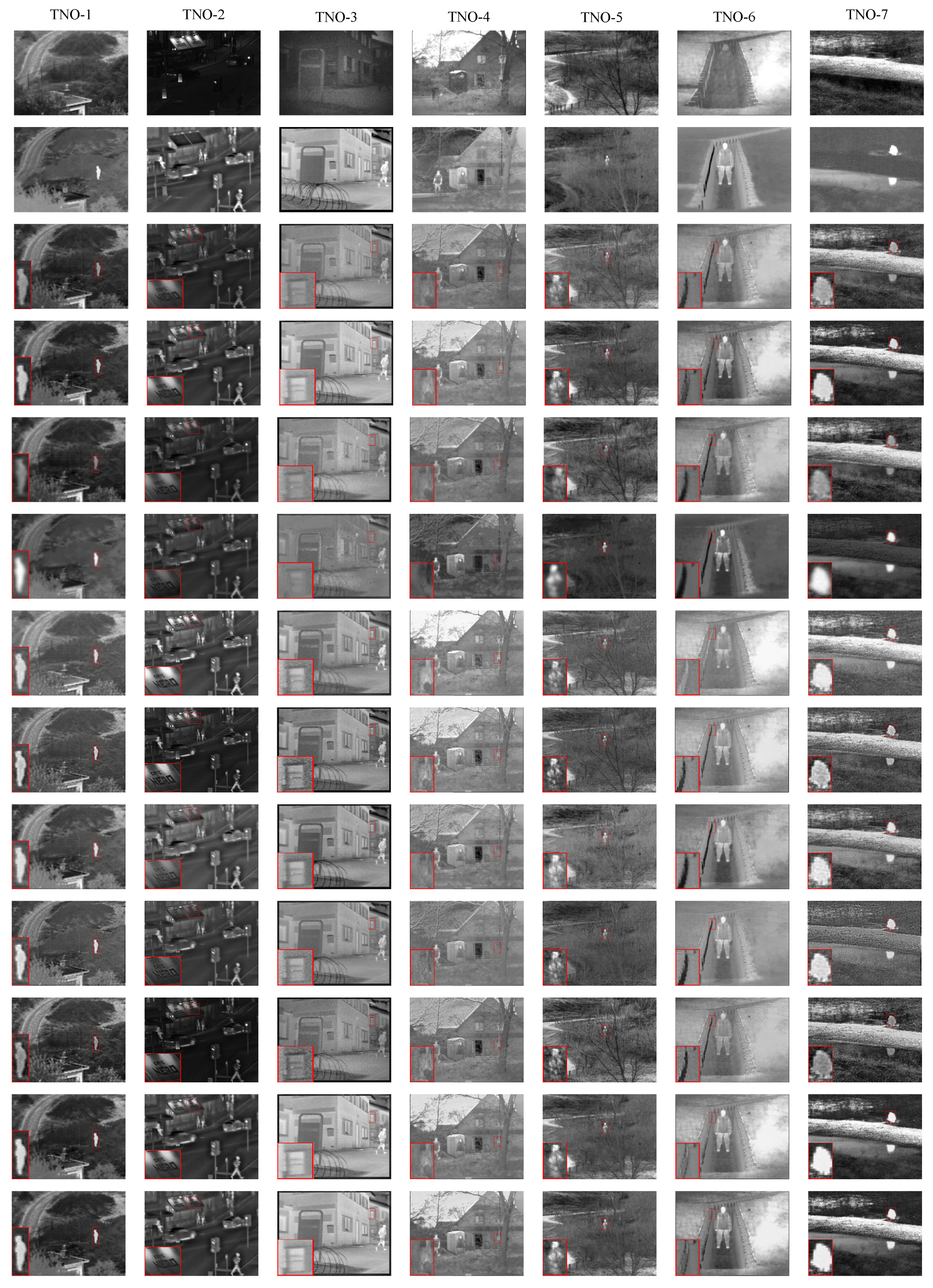
(1) TNO dataset comparison: We selected a total of 7 images for comparison and enlarged the local areas with red frames placed in the bottom left corner for subjective qualitative comparison.

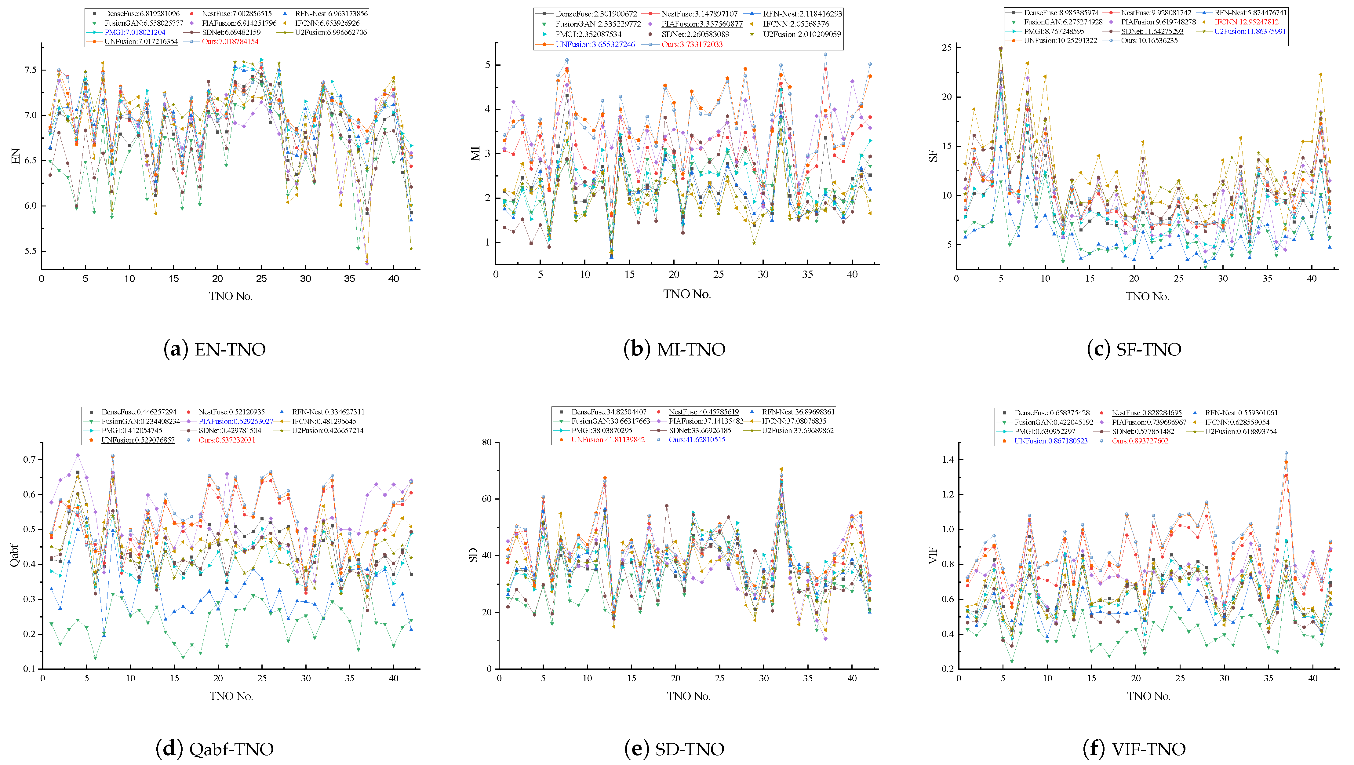
As indicated in Figure 4, the visible and infrared images are shown in the first 2 rows, while the following 11 rows represent the fusion images generated using different methods. The enlarged details of TNO-1, TNO-5, and TNO-7 clearly show that FusionGAN blurs the boundaries between human and environment, while DenseFuse and RFN-Nest exhibit weak color contrast between human and environment. In TNO-4, PMGI and SDNet exhibit low distinguishability between the sky and trees in the background environment, and the windows in the enlarged local images are also difficult to discern. The remaining images are difficult to distinguish subjectively due to significant individual variations. Therefore, we selected 42 images from this dataset for testing with the six metrics introduced above. The experimental results are presented in Figure 5. The proposed method obtains optimal results in EN, MI, Qabf and VIF, demonstrating superior performance in information preservation and visual quality of the fusion images.

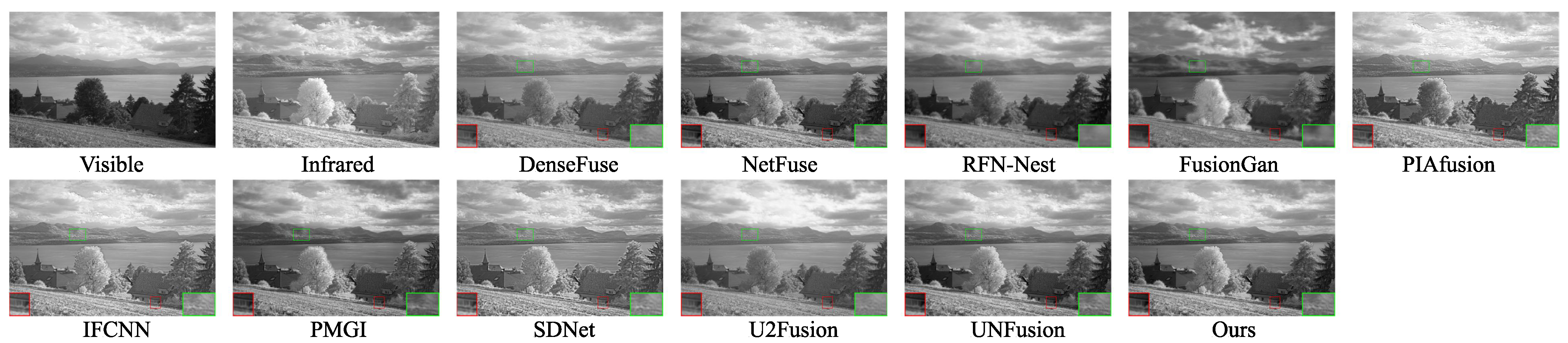
(2) NIR dataset comparison: We selected two representative images for subjective qualitative comparison. In Figure 6, the details in the enlarged sections in the bottom left (highlighted by the red box) and bottom right (highlighted by the green box) are shown. The contrast between tree colours in the fusion images from DenseFuse, RFN-Nest and U2Fusion are relatively weak, while the texture details of the distant mountains are blurred in FusionGAN.

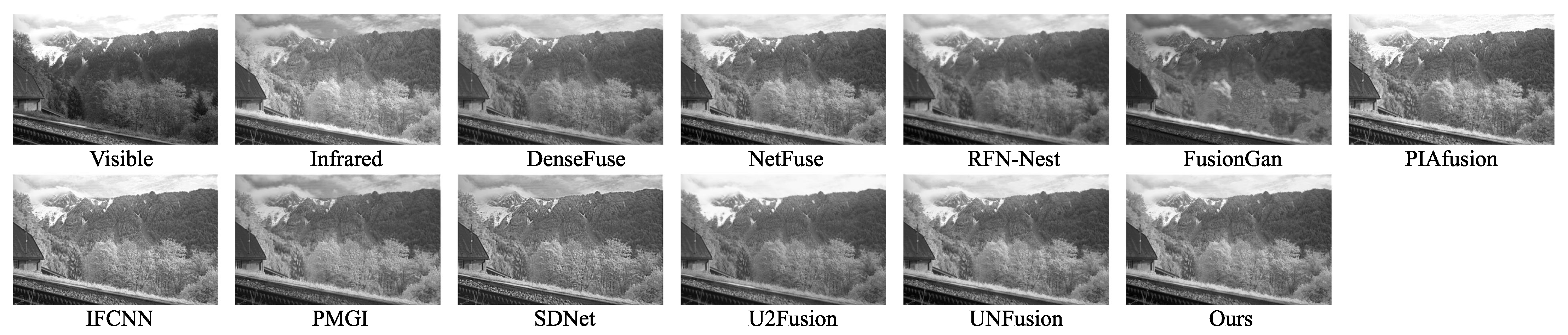
In contrast, the method proposed in this paper and the method used in UNFusion are able to better represent the details of house windows and distant grassy slopes, thus demonstrating certain visual advantages. Also, as shown in Figure 7, when fusing infrared and visible images of natural landscapes, with the exception of FusionGAN with lower clarity, the other methods generally perform well in displaying contour edge details of objects regardless of lighting conditions.

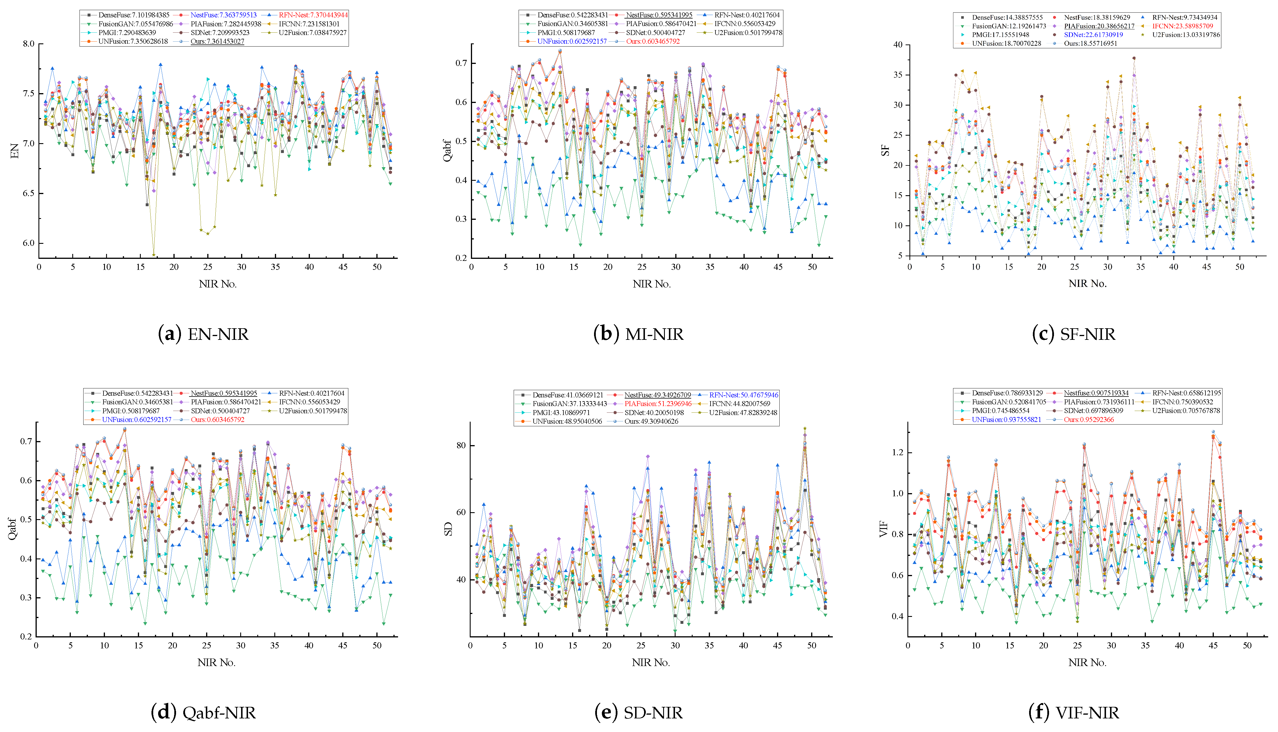
Therefore, we also used the same six metrics to quantitatively analyze and compare the 52 images in the NIR dataset. The fusion test results and experimental averages for the different methods are shown in Figure 8. Our method achieved the best scores in MI, Qabf, and VIF on this dataset, while EN and SD also performed well among the top. Meanwhile, the spatial frequency (SF) represented by SF is somewhat influenced by the downsampling and upsampling operations of the UNet++ structure; however, it still outperforms RFN-Nest and UNFusion methods based on the same architecture. This indicates that the loss of information frequency caused by sampling is effectively alleviated by our proposed method.

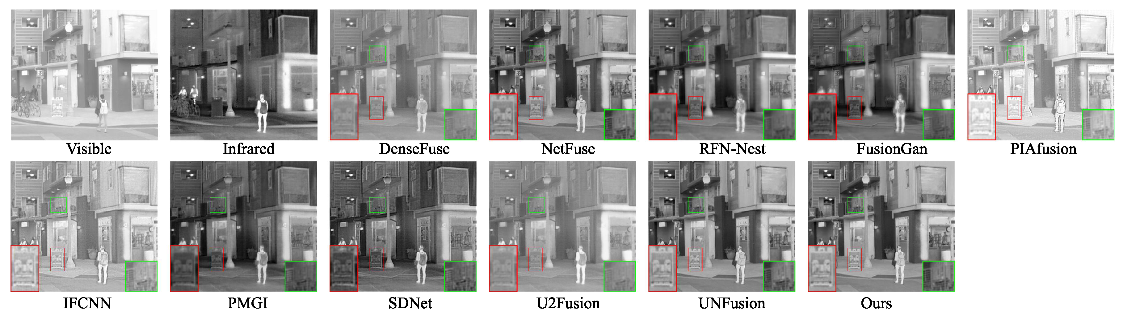
(3) RoadScene dataset comparison: We compared the performance of the fusion on 40 pairs of datasets within RoadScene. We qualitatively analyzed the above 10 methods along with the proposal method. As observed from the fusion image FLIR_00993 in Figure 9, Densefuse, PIAfusion, and U2Fusion exhibit an overall dark color tone, resulting in poor subjective visual effects for human observers and failing to effectively highlight key targets. Furthermore, FusionGAN introduces artefacts into the fused images. These artefacts can affect downstream tasks like tracking and target recognition. Similarly, in the fused image FLIR_08835 shown in Figure 10, it can be observed that PMGI and U2Fsuion fail to depict the internal structure of the firebox clearly, while SDNet exhibits blurred texture details on the person’s backpack. In contrast, our proposed method presents highly distinctive visual effects in the images, effectively distinguishing prominent targets from the background environment, which is advantageous in subsequent tasks like image segmentation and target recognition.

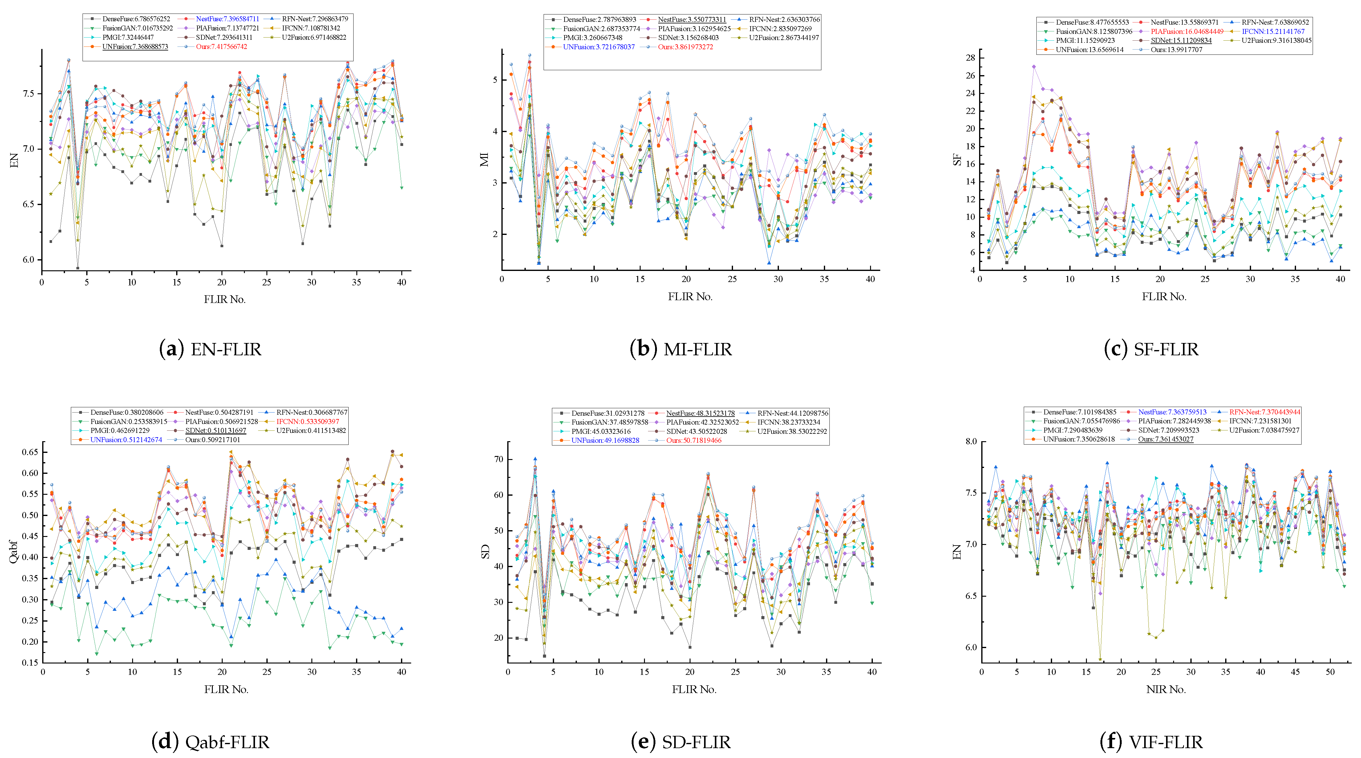
We similarly tested 40 images from the RoadScene dataset with the above six metrics, and the results are presented in Figure 11. The method also achieved the highest scores with respect to EN, MI, SD and VIF, indicating the good generalisation ability of our approach across different datasets. Furthermore, VIF achieved the highest scores across all three datasets, consistent with the qualitative observations, indicating the best match between the fusion visual quality and human perception. In summary, compared with other fusion algorithms, the proposed model can fully extract and reconstruct image features and achieve better fusion performance in extensive image tests on multiple datasets.

4.4. Computational Complexity Analysis

To comprehensively evaluate our method, we compare the computational complexity with state-of-the-art methods in terms of parameters, FLOPs, inference latency, and frames per second (FPS). All measurements were conducted on an NVIDIA GeForce RTX 4070Ti GPU with input images of size $256\times 256$.

As shown in

Table 8. Computational complexity comparison with state-of-the-art methods. Params denotes the number of parameters in millions (M), FLOPs denotes floating-point operations in giga (G), Latency is the inference time in milliseconds (ms), and FPS is frames per second. All metrics are measured with $256\times 256$ input images on an NVIDIA GeForce RTX 4070Ti GPU.

Method	Params (M)	FLOPs (G)	Latency (ms)	FPS
DenseFuse	0.0742	5.7661	1.2722	786.02
NestFuse	2.733	76.211	14.938	66.95
RFN-Nest	7.524	111.106	11.169	89.53
FusionGAN	1.327	62.519	4.049	246.94
PIAFusion	0.491	38.658	2.940	340.11
IFCNN	0.074	8.544	0.659	1518.14
PMGI	0.042	2.7661	1.773	563.99
SDNet	0.067	1.8728	0.851	1174.68
U2Fusion	0.659	43.170	2.957	338.20
UNFusion	31.122	81.789	11.044	90.55
Ours	32.513	83.140	10.652	93.87

, the compared methods can be broadly categorized into lightweight models (e.g., PMGI, SDNet, DenseFuse, IFCNN) and performance-oriented models (e.g., UNFusion, NestFuse, RFN-Nest). Our method belongs to the latter category, with 32.513M parameters and 83.140G FLOPs. While this computational cost is higher than lightweight methods, our model is specifically designed to achieve superior fusion quality through the integration of Restormer blocks and multi-dimensional attention mechanisms.

Notably, compared to UNFusion, which achieves similar high-quality fusion performance, our method has comparable model size but achieves faster inference speed (93.87 FPS vs. 90.55 FPS), indicating that our architecture design is more computationally efficient. Our method also outperforms other attention-enhanced approaches such as NestFuse (66.95 FPS) and RFN-Nest (89.53 FPS) in terms of inference speed while delivering superior fusion quality, as demonstrated in Section 4.3. The inference speed of 93.87 FPS is sufficient for real-time applications including video surveillance and autonomous driving scenarios. Combined with the significant improvements in fusion quality metrics (MI, VIF, Qabf) and visual quality demonstrated in our experiments, we believe the computational cost of our method is justified by its performance gains.

5. Conclusions

In this paper, we proposed MRMAFusion, a multi-scale Restormer and multi-dimensional attention model based on nested connections for infrared and visible image fusion. Built on the UNet++ architecture, our model employs multi-scale Restormers and convolutional blocks during vertical downsampling to jointly extract features and reduce global information loss. Both the encoder and decoder use nested connections horizontally. The convolutional encoder blocks incorporate the SimAM attention mechanism to train 3D attention weights, and both spatial and channel attention for fusing infrared and visible image features, enhancing the model’s feature extraction capability through multi-dimensional attention mechanism. We design loss functions and conduct comparative experiments to select coefficients for loss terms, and conduct ablation experiments to prove the efficacy of our proposed RTB block and multi-dimensional attention mechanism. MRMAFusion compares qualitatively and quantitatively with ten state-of-the-art fusion methods on three datasets: TNO, NIR, and RoadScene. The experimental results indicate that MRMAFusion has superior fusion visual effects and metric advantages. In future work, we will explore model compression techniques such as knowledge distillation and network pruning to reduce the computational overhead while maintaining fusion performance. We also plan to integrate other advanced deep learning methods to further optimize the model structure, extending its applicability to resource-constrained devices and other domains such as medical image fusion and remote sensing image fusion.

References

1. Zhang, X.; Demiris, Y. Visible and infrared image fusion using deep learning. IEEE Trans. Pattern Anal. Mach. Intell. 2023, 45, 10535–10554. [Google Scholar] [CrossRef]
2. Zhang, Y.; Liu, Y.; Sun, P.; Yan, H.; Zhao, X.; Zhang, L. IFCNN: A general image fusion framework based on convolutional neural network. Inf. Fusion 2020, 54, 99–118. [Google Scholar] [CrossRef]
3. Kang, X.; Yin, H.; Duan, P. Global–local feature fusion network for visible–infrared vehicle detection. IEEE Geosci. Remote Sens. Lett. 2024, 21, 1–5. [Google Scholar] [CrossRef]
4. Chen, J.; Ding, J.; Ma, J. HitFusion: Infrared and visible image fusion for high-level vision tasks using transformer. IEEE Trans. Multimed. 2024, 26, 10145–10159. [Google Scholar] [CrossRef]
5. Zhang, X.; Ye, P.; Leung, H.; Gong, K.; Xiao, G. Object fusion tracking based on visible and infrared images: A comprehensive review. Inf. Fusion 2020, 63, 166–187. [Google Scholar] [CrossRef]
6. Chen, J.; Li, X.; Luo, L.; Mei, X.; Ma, J. Infrared and visible image fusion based on target-enhanced multiscale transform decomposition. Inf. Sci. 2020, 508, 64–78. [Google Scholar] [CrossRef]
7. Luo, X.; Zhang, Z.; Zhang, B.; Wu, X. Image fusion with contextual statistical similarity and nonsubsampled shearlet transform. IEEE Sens. J. 2016, 17, 1760–1771. [Google Scholar] [CrossRef]
8. Liu, Y.; Yang, X.; Zhang, R.; Albertini, M.K.; Celik, T.; Jeon, G. Entropy-based image fusion with joint sparse representation and rolling guidance filter. Entropy 2020, 22, 118. [Google Scholar] [CrossRef]
9. Zhang, Q.; Li, G.; Cao, Y.; Han, J. Multi-focus image fusion based on non-negative sparse representation and patch-level consistency rectification. Pattern Recognit. 2020, 104, 107325. [Google Scholar] [CrossRef]
10. Ma, J.; Zhou, Z.; Wang, B.; Zong, H. Infrared and visible image fusion based on visual saliency map and weighted least square optimization. Infrared Phys. Technol. 2017, 82, 8–17. [Google Scholar] [CrossRef]
11. Li, H.; Wu, X.J. DenseFuse: A fusion approach to infrared and visible images. IEEE Trans. Image Process. 2018, 28, 2614–2623. [Google Scholar] [CrossRef] [PubMed]
12. Li, H.; Wu, X.J.; Durrani, T. NestFuse: An infrared and visible image fusion architecture based on nest connection and spatial/channel attention models. IEEE Trans. Instrum. Meas. 2020, 69, 9645–9656. [Google Scholar] [CrossRef]
13. Li, H.; Wu, X.J.; Kittler, J. RFN-Nest: An end-to-end residual fusion network for infrared and visible images. Inf. Fusion 2021, 73, 72–86. [Google Scholar] [CrossRef]
14. Zhao, Z.; Xu, S.; Zhang, C.; Liu, J.; Zhang, J.; Li, P. DIDFuse: Deep image decomposition for infrared and visible image fusion. In Proceedings of the Twenty-Ninth International Joint Conference on Artificial Intelligence, Yokohama, Japan, 11–17 July 2020; pp. 970–976. [Google Scholar]
15. Wang, Z.; Wang, J.; Wu, Y.; Xu, J.; Zhang, X. UNFusion: A unified multi-scale densely connected network for infrared and visible image fusion. IEEE Trans. Circuits Syst. Video Technol. 2021, 32, 3360–3374. [Google Scholar] [CrossRef]
16. Zhang, H.; Xu, H.; Xiao, Y.; Guo, X.; Ma, J. Rethinking the image fusion: A fast unified image fusion network based on proportional maintenance of gradient and intensity. Proc. Aaai Conf. Artif. Intell. 2020, 34, 12797–12804. [Google Scholar] [CrossRef]
17. Xu, H.; Ma, J.; Le, Z.; Jiang, J.; Guo, X. FusionDN: A unified densely connected network for image fusion. Proc. Aaai Conf. Artif. Intell. 2020, 34, 12484–12491. [Google Scholar] [CrossRef]
18. Xu, H.; Ma, J.; Jiang, J.; Guo, X.; Ling, H. U2Fusion: A unified unsupervised image fusion network. IEEE Trans. Pattern Anal. Mach. Intell. 2020, 44, 502–518. [Google Scholar] [CrossRef]
19. Ma, J.; Yu, W.; Liang, P.; Li, C.; Jiang, J. FusionGAN: A generative adversarial network for infrared and visible image fusion. Inf. Fusion 2019, 48, 11–26. [Google Scholar] [CrossRef]
20. Ma, J.; Xu, H.; Jiang, J.; Mei, X.; Zhang, X.P. DDcGAN: A dual-discriminator conditional generative adversarial network for multi-resolution image fusion. IEEE Trans. Image Process. 2020, 29, 4980–4995. [Google Scholar] [CrossRef]
21. Ma, J.; Tang, L.; Fan, F.; Huang, J.; Mei, X.; Ma, Y. SwinFusion: Cross-domain long-range learning for general image fusion via swin transformer. IEEE/CAA J. Autom. Sin. 2022, 9, 1200–1217. [Google Scholar] [CrossRef]
22. Wang, Z.; Chen, Y.; Shao, W.; Li, H.; Zhang, L. SwinFuse: A residual swin transformer fusion network for infrared and visible images. IEEE Trans. Instrum. Meas. 2022, 71, 1–12. [Google Scholar] [CrossRef]
23. Tang, W.; He, F.; Liu, Y.; Duan, Y.; Si, T. DATFuse: Infrared and visible image fusion via dual attention transformer. IEEE Trans. Circuits Syst. Video Technol. 2023, 33, 3159–3172. [Google Scholar] [CrossRef]
24. Luo, X.; Wang, J.; Zhang, Z.; Wu, X.J. A full-scale hierarchical encoder-decoder network with cascading edge-prior for infrared and visible image fusion. Pattern Recognit. 2024, 148, 110192. [Google Scholar] [CrossRef]
25. Zhou, Z.; Siddiquee, M.M.R.; Tajbakhsh, N.; Liang, J. UNet++: Redesigning skip connections to exploit multiscale features in image segmentation. IEEE Trans. Med. Imaging 2019, 39, 1856–1867. [Google Scholar] [CrossRef]
26. Zamir, S.W.; Arora, A.; Khan, S.; Hayat, M.; Khan, F.S.; Yang, M.H. Restormer: Efficient transformer for high-resolution image restoration. In Proceedings of the IEEE/CVF Conference on Computer Vision and Pattern Recognition, New Orleans, LA, USA, 18–24 June 2022; pp. 5728–5739. [Google Scholar]
27. Yang, L.; Zhang, R.Y.; Li, L.; Xie, X. SimAM: A simple, parameter-free attention module for convolutional neural networks. In Proceedings of the International Conference on Machine Learning, PMLR, Virtual, 18–24 July 2021; pp. 11863–11874. [Google Scholar]
28. Liu, Y.; Chen, X.; Ward, R.K.; Wang, Z.J. Image fusion with convolutional sparse representation. IEEE Signal Process. Lett. 2016, 23, 1882–1886. [Google Scholar] [CrossRef]
29. Vaswani, A.; Shazeer, N.; Parmar, N.; Uszkoreit, J.; Jones, L.; Gomez, A.N.; Kaiser, L.; Polosukhin, I. Attention is all you need. In Proceedings of the Advances in Neural Information Processing Systems 30, Long Beach, CA, USA, 4–9 December 2017. [Google Scholar]
30. Liu, Z.; Lin, Y.; Cao, Y.; Hu, H.; Wei, Y.; Zhang, Z.; Lin, S.; Guo, B. Swin transformer: Hierarchical vision transformer using shifted windows. In Proceedings of the IEEE/CVF International Conference on Computer Vision, Montreal, QC, Canada, 11–17 October 2021; pp. 10012–10022. [Google Scholar]
31. Su, W.; Huang, Y.; Li, Q.; Zuo, F.; Liu, L. Infrared and visible image fusion based on adversarial feature extraction and stable image reconstruction. IEEE Trans. Instrum. Meas. 2022, 71, 104853. [Google Scholar] [CrossRef]
32. Liu, J.; Sun, G.; Zheng, B.; Dong, L. TCIGFusion: A two-stage correlated feature interactive guided network for infrared and visible image fusion. Opt. Lasers Eng. 2025, 195, 109265. [Google Scholar] [CrossRef]
33. Liu, J.; Sun, G.; Zheng, B.; Dong, L. TSDGFusion: A text and semantic dual-guided model for infrared and visible image fusion. Displays 2025, 91, 103266. [Google Scholar] [CrossRef]
34. Li, H.; Wu, X.J. CrossFuse: A novel cross attention mechanism based infrared and visible image fusion approach. Inf. Fusion 2024, 103, 102147. [Google Scholar] [CrossRef]
35. Woo, S.; Park, J.; Lee, J.Y.; Kweon, I.S. CBAM: Convolutional block attention module. In Proceedings of the European Conference on Computer Vision (ECCV), Munich, Germany, 8–14 September 2018; pp. 3–19. [Google Scholar]
36. Li, J.; Huo, H.; Li, C.; Wang, R.; Feng, Q. AttentionFGAN: Infrared and visible image fusion using attention-based generative adversarial networks. IEEE Trans. Multimed. 2020, 23, 1383–1396. [Google Scholar] [CrossRef]
37. Tang, X.; Zhao, J.; Cui, G.; Tian, H.; Shi, Z.; Hou, C. MFAGAN: A multiscale feature-attention generative adversarial network for infrared and visible image fusion. Infrared Phys. Technol. 2023, 133, 104796. [Google Scholar] [CrossRef]
38. Liu, X.; Wang, R.; Huo, H.; Yang, X.; Li, J. An attention-guided and wavelet-constrained generative adversarial network for infrared and visible image fusion. Infrared Phys. Technol. 2023, 129, 104570. [Google Scholar] [CrossRef]
39. Wang, Y.; Pu, J.; Miao, D.; Zhang, L.; Zhang, L.; Du, X. SCGRFuse: An infrared and visible image fusion network based on spatial/channel attention mechanism and gradient aggregation residual dense blocks. Eng. Appl. Artif. Intell. 2024, 132, 107898. [Google Scholar] [CrossRef]
40. Lou, M.; Zhang, S.; Zhou, H.Y.; Yang, S.; Wu, C.; Yu, Y. TransXNet: Learning both global and local dynamics with a dual dynamic token mixer for visual recognition. IEEE Trans. Neural Netw. Learn. Syst. 2025, 36, 11534–11547. [Google Scholar] [CrossRef]
41. Liu, Z.; Blasch, E.; Xue, Z.; Zhao, J.; Laganiere, R.; Wu, W. Objective assessment of multiresolution image fusion algorithms for context enhancement in night vision: A comparative study. IEEE Trans. Pattern Anal. Mach. Intell. 2011, 34, 94–109. [Google Scholar] [CrossRef]
42. Roberts, J.W.; Van Aardt, J.A.; Ahmed, F.B. Assessment of image fusion procedures using entropy, image quality, and multispectral classification. J. Appl. Remote Sens. 2008, 2, 023522. [Google Scholar]
43. Eskicioglu, A.M.; Fisher, P.S. Image quality measures and their performance. IEEE Trans. Commun. 1995, 43, 2959–2965. [Google Scholar] [CrossRef]
44. Rao, Y.J. In-fibre Bragg grating sensors. Meas. Sci. Technol. 1997, 8, 355. [Google Scholar] [CrossRef]
45. Piella, G.; Heijmans, H. A new quality metric for image fusion. In Proceedings of the 2003 International Conference on Image Processing, Barcelona, Spain, 14–17 September 2003; Volume 3, pp. 173–176. [Google Scholar]
46. Han, Y.; Cai, Y.; Cao, Y.; Xu, X. A new image fusion performance metric based on visual information fidelity. Inf. Fusion 2013, 14, 127–135. [Google Scholar] [CrossRef]
47. Tang, L.; Yuan, J.; Zhang, H.; Jiang, X.; Ma, J. PIAFusion: A progressive infrared and visible image fusion network based on illumination aware. Inf. Fusion 2022, 83, 79–92. [Google Scholar] [CrossRef]
48. Zhang, H.; Ma, J. SDNet: A versatile squeeze-and-decomposition network for real-time image fusion. Int. J. Comput. Vis. 2021, 129, 2761–2785. [Google Scholar] [CrossRef]
Figure 1. Overall architecture of the proposed MRMAFusion network. (a) The complete encoder–decoder framework with nested connections; (b) RTB (Restormer Transformer Block) module structure; (c) ESB (Encoder SimAM Block) module structure.
Applsci 16 00946 g001
Figure 2. Multi-scale depthwise convolutional structure.
Applsci 16 00946 g002
Figure 3. Fusion of spatial and channel attention weighted models.
Applsci 16 00946 g003
Figure 4. Qualitative experimental comparisons of seven typical infrared and visible TNO images. (From top to bottom are visible, infrared, DenseFuse, NestFuse, RFN-Nest, FusionGAN, PIAFusion, IFCNN, PMGI, SDNet, U2Fusion, UNFusion and ours).
Applsci 16 00946 g004
Figure 5. Results of the 6 objective parameters for the proposed method and 10 other methods on 42 images in the TNO dataset (red represents the best, blue the second best and underlined the third highest).
Applsci 16 00946 g005
Figure 6. Qualitative experimental comparison of NIR-1 images.
Applsci 16 00946 g006
Figure 7. Qualitative experimental comparison of NIR-2 images.
Applsci 16 00946 g007
Figure 8. Results of the 6 objective parameters for the proposed method and 10 other methods on 52 images in the NIR dataset (red represents the best, blue the second best and underlined the third highest).
Applsci 16 00946 g008
Figure 9. Qualitative experimental comparison of FLIR_00993 images.
Applsci 16 00946 g009
Figure 10. Qualitative experimental comparison of FLIR_08835 images.
Applsci 16 00946 g010
Figure 11. Results of the 6 objective parameters for the proposed method and 10 other methods on 40 images in the RoadScene dataset (red represents the best, blue the second best and underlined the third highest).
Applsci 16 00946 g011