Fuzzy Model-Based Output Constraint Satisfaction Mechanism for Controllers of Nonlinear Processes


Abstract
1. Introduction
2. Materials and Methods
2.1. Obtaining the Fuzzy Process Model
- 1.
- The decision regarding the number and location of operating points, near which the responses will be collected, is made. An analysis of the steady-state characteristic may be useful to choose these operating points appropriately. Let us denote the number of the collected responses as l.
- 2.
- The step responses are obtained near each operating point chosen in point no. 1. The coefficients of the step responses are collected until they do not significantly change. Once the changes between the collected coefficients become negligible, obtaining the response is finished. Let denote the length of the longest step response. It will be the parameter called the dynamics horizon of the constructed fuzzy model. Thus, in the current step, coefficients of step responses are collected, where f is the index of the operating point near which the step response is collected.
- 3.
- From the collected step response coefficients, the output value from which the step response generation started () is subtracted:
- 4.
- When collecting the step responses of a nonlinear process, the change in the manipulated variable that can be applied may be different to due to the nonlinearity of the process. However, all step responses in the constructed fuzzy model need to be compatible and be responses to the step change by in the manipulated variable. Therefore, the responses to changes of other magnitudes than 1 must be scaled. Thus, the following formula is applied to each step response coefficient:where is the size of the step change in the manipulated variable applied to collect the step response.
- 5.
- The collected and scaled step responses are combined to obtain the fuzzy model.
2.2. Output Constraint Satisfaction Mechanism
- –
- If , then
- –
- If , then
- –
- If , then
- –
- If , then
2.3. Taking Modeling Uncertainty into Account
- –
- If , then
- –
- If , then
- –
- If , then
- –
- If , then
3. Results
3.1. Example Control System
3.2. Obtaining Simplified Process Model
3.3. Experiments
4. Discussion & Conclusions
- Obtain a higher quality of the product, thanks to the fulfillment of quality constraints;
- Reduce losses when avoiding (or limiting the occurrence of) situations where the product does not meet the requirements in the event of exceeding the constraints;
- Obtain economic benefits resulting from the above points.
Author Contributions
Funding
Institutional Review Board Statement
Informed Consent Statement
Data Availability Statement
Conflicts of Interest
Abbreviations
| CE1 | Control Effort Indicator 1 |
| CE2 | Control Effort Indicator 2 |
| LMPC | MPC Based on Linear Lodel |
| MPC | Model Predictive Control |
| NMPC | Nonlinear MPC |
| PID | Proportional–Integral–Derivative |
| SAE | Sum of Absolute Errors |
| SSE | Sum of Squared Errors |
References
- Yuan, M.; Manzie, C.; Good, M.; Shames, I.; Gan, L.; Keynejad, F.; Robinette, T. A Review of Industrial Tracking Control Algorithms. Control Eng. Pract. 2020, 102, 104536. [Google Scholar]
- Yuan, M.; Manzie, C.; Good, M.; Shames, I.; Gan, L.; Keynejad, F.; Robinette, T. Error–Bounded Reference Tracking MPC for Machines With Structural Flexibility. IEEE Trans. Ind. Electron. 2020, 67, 8143–8154. [Google Scholar]
- Garone, E.; Di Cairano, S.; Kolmanovsky, I. Reference and Command Governors for Systems with Constraints: A Survey on Theory and Applications. Automatica 2017, 75, 306–328. [Google Scholar] [CrossRef]
- Nebeluk, R.; Ławryńczuk, M. Tuning of Nonlinear MPC Algorithm for Vehicle Obstacle Avoidance. In Advanced, Contemporary Control. Advances in Intelligent Systems and Computing; Bartoszewicz, A., Kabziński, J., Kacprzyk, J., Eds.; Springer: Cham, Switzerland, 2020; Volume 1196, pp. 595–615. [Google Scholar]
- Perera, Y.S.; Li, J.; Abeykoon, C. Melt Viscosity Control in Polymer Extrusion Using Nonlinear Model Predictive Control with Neural State Space Modelling and Soft Sensor Feedback. J. Process Control 2025, 155, 103556. [Google Scholar]
- Tatjewski, P. Offset–Free Nonlinear Model Predictive Control with State–Space Process Models. Arch. Control Sci. 2017, 27, 595–615. [Google Scholar] [CrossRef]
- Schäfer, A.; Kühl, P.; Diehl, M.; Schlöder, J.; Bock, H.G. Fast Reduced Multiple Shooting Methods for Nonlinear Model Predictive Control. Chem. Eng. Process. 2007, 46, 1200–1214. [Google Scholar] [CrossRef]
- Zavala, V.M.; Laird, C.D.; Biegler, L.T. A Fast Moving Horizon Estimation Algorithm Based on Nonlinear Programming Sensitivity. J. Process Control 2008, 18, 876–884. [Google Scholar]
- Ławryńczuk, M.; Nebeluk, R. Beyond the Quadratic Norm: Computationally Efficient Constrained Nonlinear MPC Using a Custom Cost Function. ISA Trans. 2023, 134, 336–356. [Google Scholar]
- Marusak, P.M. Designing Efficient Model Predictive Control Algorithm Using Easy–to–Obtain Fuzzy Models. Int. J. Electron. Telecommun. 2025, 71, 1–8. [Google Scholar]
- Nebeluk, R.; Ławryńczuk, M. Computationally Simple Nonlinear MPC Algorithm for Vehicle Obstacle Avoidance With Minimization of Fuel Utilization. IEEE Access 2021, 9, 17296–17311. [Google Scholar] [CrossRef]
- Dominguez, L.F.; Pistikopoulos, E.N. A Novel mp-NLP Algorithm for Explicit/Multi-parametric NMPC. In Proceedings of the 8th IFAC Symposium on Nonlinear Control Systems, Bologna, Italy, 1–3 September 2010. [Google Scholar]
- Johansen, T.A. On multi–parametric nonlinear programming and explicit nonlinear model predictive control. In Proceedings of the 41st IEEE Conference on Decision and Control, Las Vegas, NV, USA, 10–13 December 2002; Volume 3, pp. 2768–2773. [Google Scholar]
- Johansen, T.A. Approximate explicit receding horizon control of constrained nonlinear systems. Automatica 2004, 40, 293–300. [Google Scholar] [CrossRef]
- Bemporad, A.; Borrelli, F.; Morari, M. Piecewise linear optimal controllers for hybrid systems. In Proceedings of the 2000 American Control Conference, Chicago, IL, USA, 28–30 June 2000; Volume 2, pp. 1190–1194. [Google Scholar]
- Bemporad, A.; Morari, M.; Dua, V.; Pistikopoulos, E.N. The explicit linear quadratic regulator for constrained systems. Automatica 2002, 38, 3–20. [Google Scholar] [CrossRef]
- Pistikopoulos, E.N.; Dua, V.; Bozinis, N.A.; Bemporad, A.; Morari, M. On–line optimization via off–line parametric optimization tools. Comput. Chem. Eng. 2002, 26, 175–185. [Google Scholar] [CrossRef]
- Chaber, P.; Ławryńczuk, M. Fast Analytical Model Predictive Controllers and Their Implementation for STM32 ARMmicrocontroller. IEEE Trans. Ind. Inform. 2019, 15, 4580–4590. [Google Scholar] [CrossRef]
- Wojtulewicz, A.; Ławryńczuk, M. Computationally Efficient Implementation of Dynamic Matrix Control Algorithm for Very Fast Processes Using Programmable Logic Controller. In Proceedings of the 23rd International Conference on Methods and Models in Automation and Robotics (MMAR), Międzyzdroje, Poland, 27–30 August 2018; pp. 579–584. [Google Scholar]
- Marusak, P.M.; Kuntanapreeda, S. Output Constrained IMC Controllers In Control Systems of Electromechanical Actuators. Control Theory Technol. 2015, 13, 245–255. [Google Scholar] [CrossRef]
- Piegat, A. Fuzzy Modeling and Control; Physica–Verlag: Heidelberg, Germany, 2001. [Google Scholar]
- Takagi, T.; Sugeno, M. Fuzzy Identification of Systems and Its Application to Modeling and Control. IEEE Trans. Syst. Man Cybern. 1985, 15, 116–132. [Google Scholar] [CrossRef]
- Li, J.; Lewis, H.W. Fuzzy Clustering Algorithms—Review of the Applications. In Proceedings of the 2016 IEEE International Conference on Smart Cloud (SmartCloud), New York, NY, USA, 18–20 November 2016; pp. 282–288. [Google Scholar]
- Tatjewski, P. Advanced Control of Industrial Processes: Structures and Algorithms; Springer: London, UK, 2007. [Google Scholar]
- Marusak, P.M. Analytical MPC Algorithm Using Steady-State Process Model. Algorithms 2025, 18, 79. [Google Scholar] [CrossRef]
- Okienková, K.; Dodek, M.; Málik, R.; Paulusová, J.; Tárník, M. Robust Model Predictive Control of the Van De Vusse Reaction with Uncertain Extended Prediction Model and LMI–Based Design. IEEE Access 2025, 13, 182088–182106. [Google Scholar] [CrossRef]
- Krishna, D.; Suryanarayana, K.; Aparna, G.; Padma Sree, R. Tuning of PID controllers for continuous stirred tank reactors. Indian Chemical Engineer 2012, 54, 157–179. [Google Scholar] [CrossRef]
- Marusak, P.M. A numerically efficient fuzzy MPC algorithm with fast generation of the control signal. Int. J. Appl. Math. Comput. Sci. 2021, 31, 59–71. [Google Scholar] [CrossRef]
- Doyle, F.; Ogunnaike, B.A.; Pearson, R.K. Nonlinear Model–Based Control Using Second–Order Volterra Models. Automatica 1995, 31, 697–714. [Google Scholar] [CrossRef]

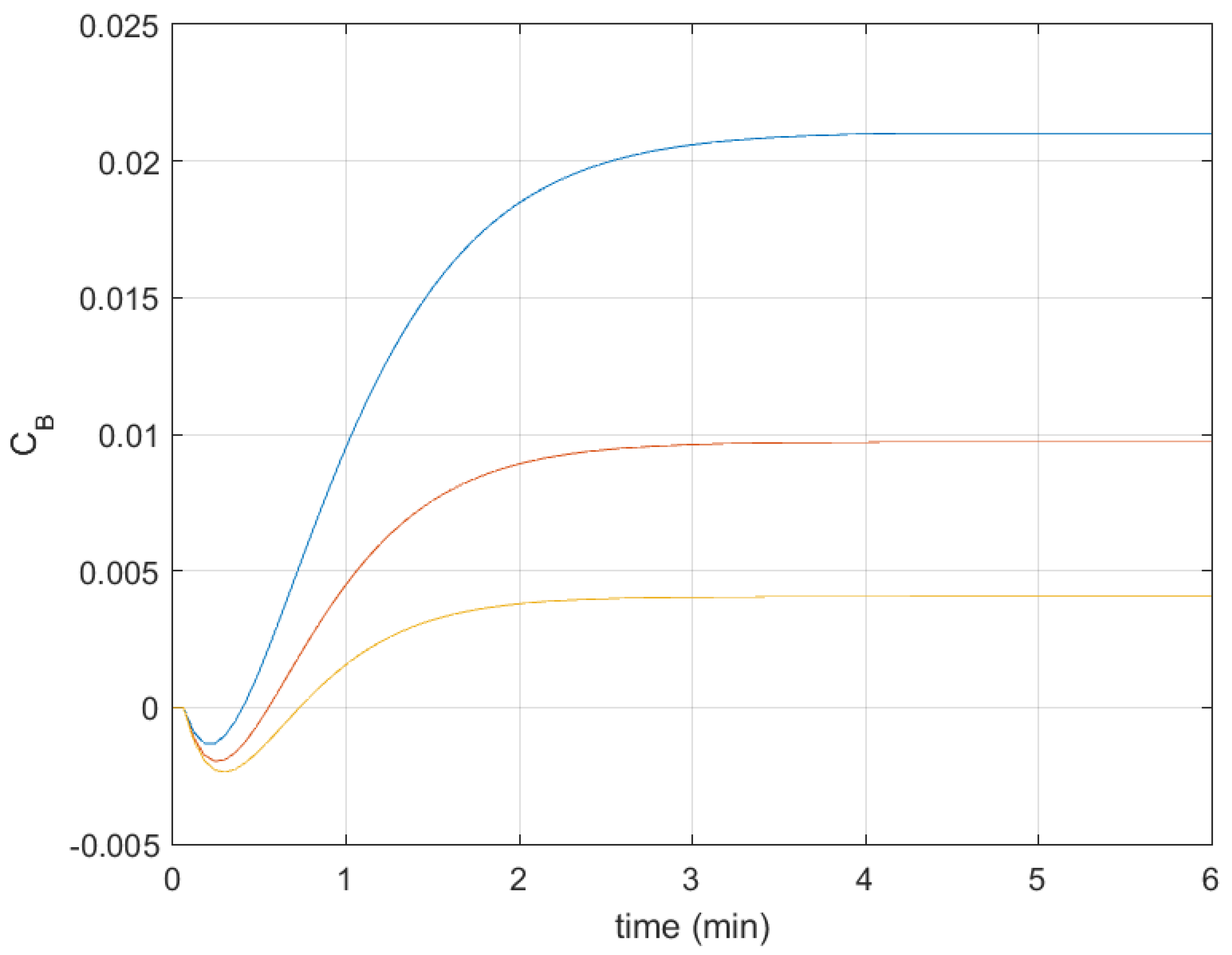






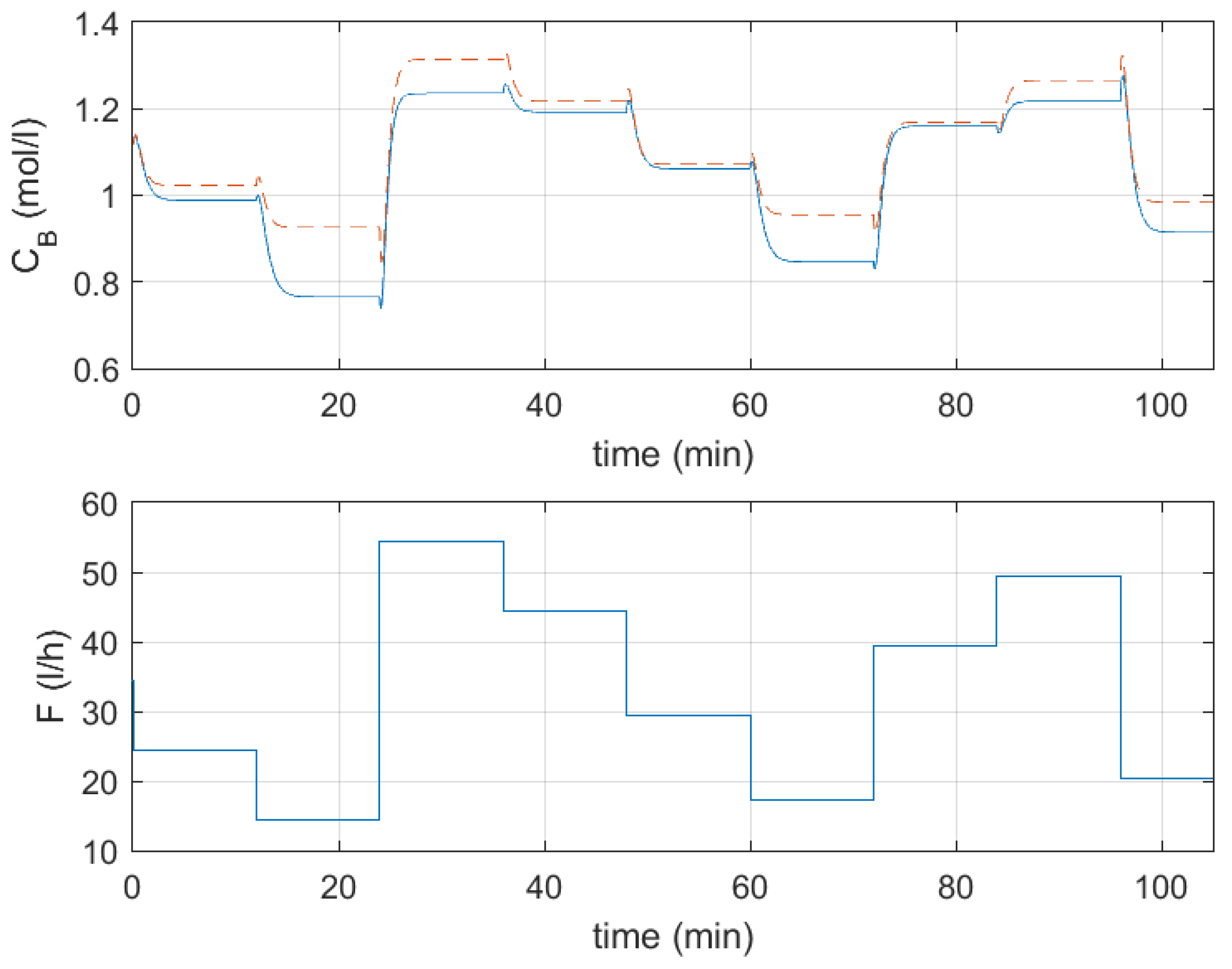
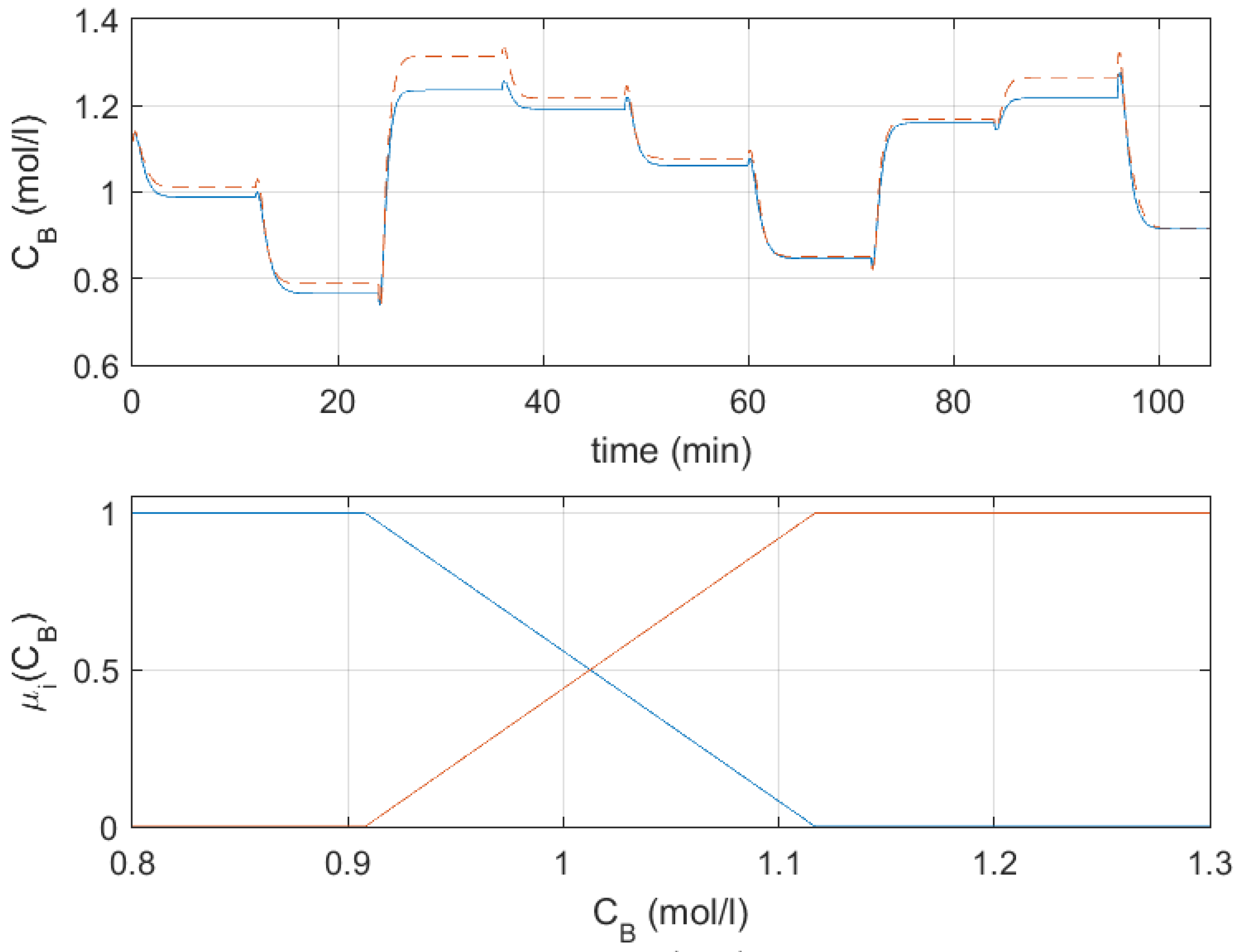
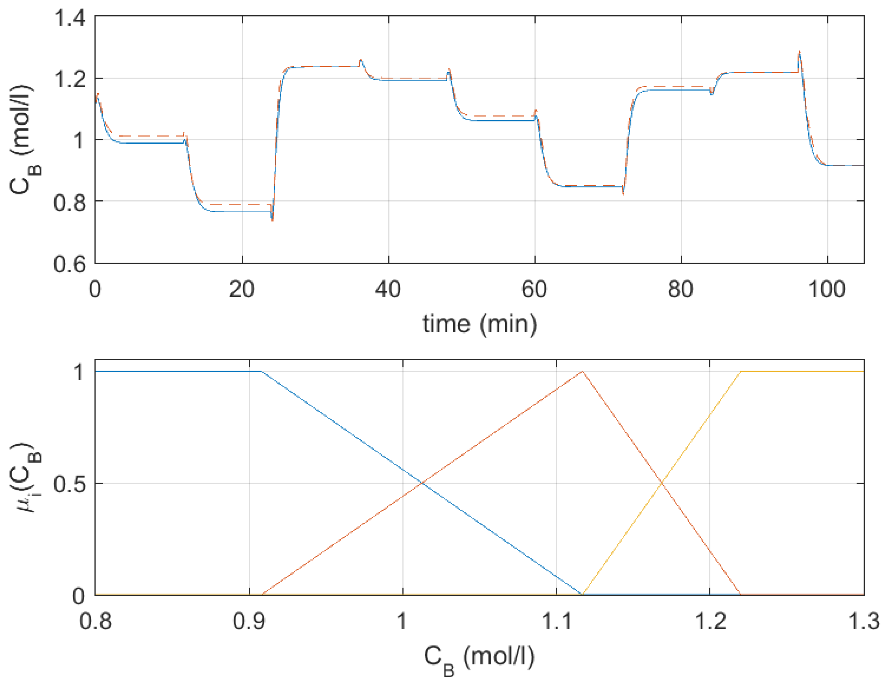
| One Local Model (Figure 3) | Two Local Models (Figure 4) | Three Local Models (Figure 5) |
|---|---|---|
| 9.3097 | 2.0013 | 0.3568 |
| Parameter | Local Model #1 (f = 1) | Local Model #2 (f = 2) | Local Model #3 (f = 3) |
|---|---|---|---|
| 0.91 | 1.12 | 1.22 | |
| 20.10 | 34.30 | 49.98 |
| Response | Overshoot (%) | (min) | SSE | SAE | CE2 | CE1 | |
|---|---|---|---|---|---|---|---|
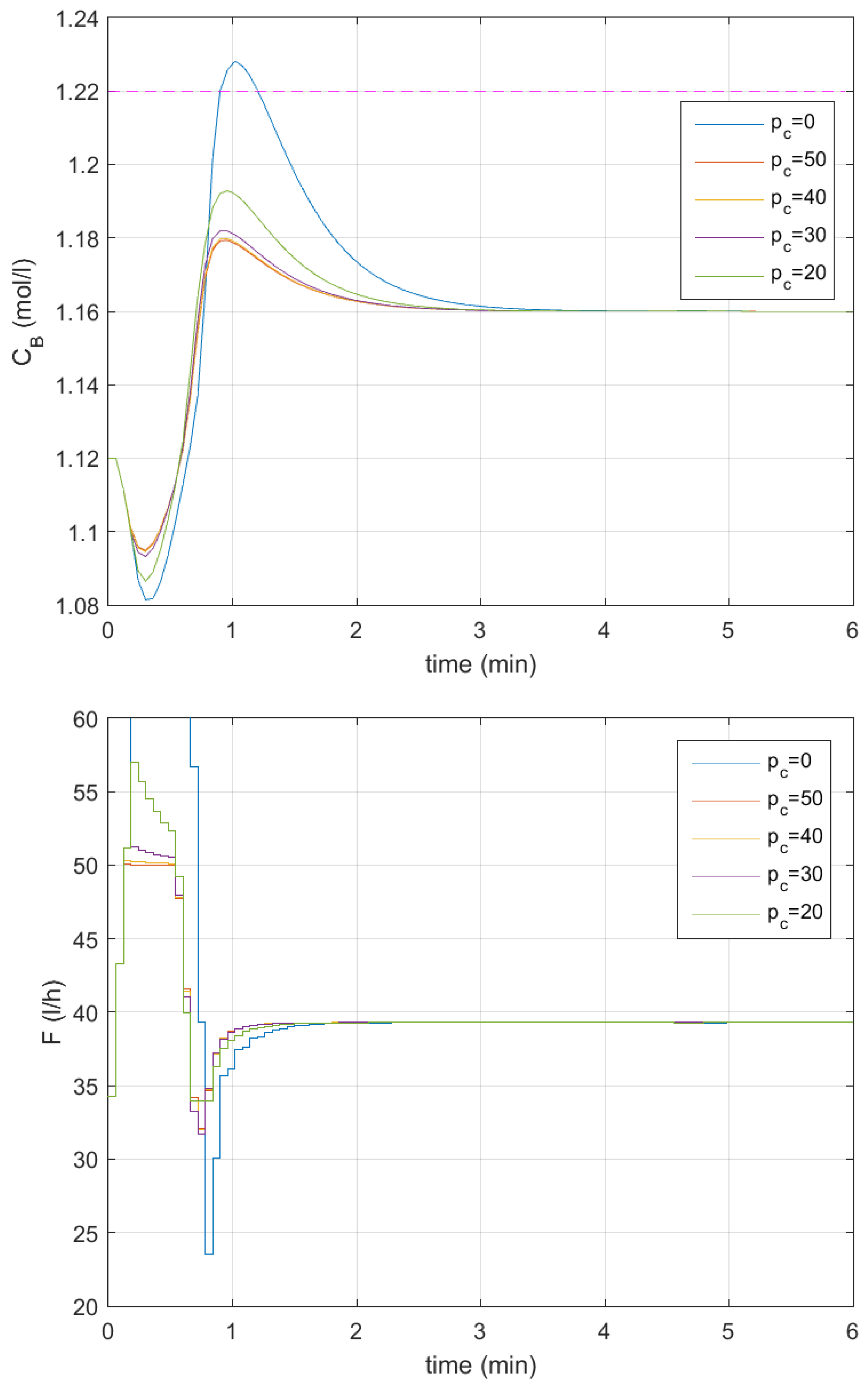
| 0 | Figure 6 blue lines | 170.24 | 2.82 | 0.0869 | 1.6704 | 860.3386 | 78.0063 |
| 50–70 | Figure 6 red lines | 48.27 | 2.10 | 0.0349 | 0.8442 | 242.6855 | 40.8727 |
| 40 | Figure 6 yellow lines | 49.41 | 2.10 | 0.0351 | 0.8500 | 249.2133 | 41.5072 |
| 30 | Figure 6 lilac lines | 54.70 | 2.16 | 0.0364 | 0.8772 | 277.9110 | 43.9890 |
| 20 | Figure 6 green lines | 82.11 | 2.34 | 0.0449 | 1.0468 | 320.7838 | 51.1836 |
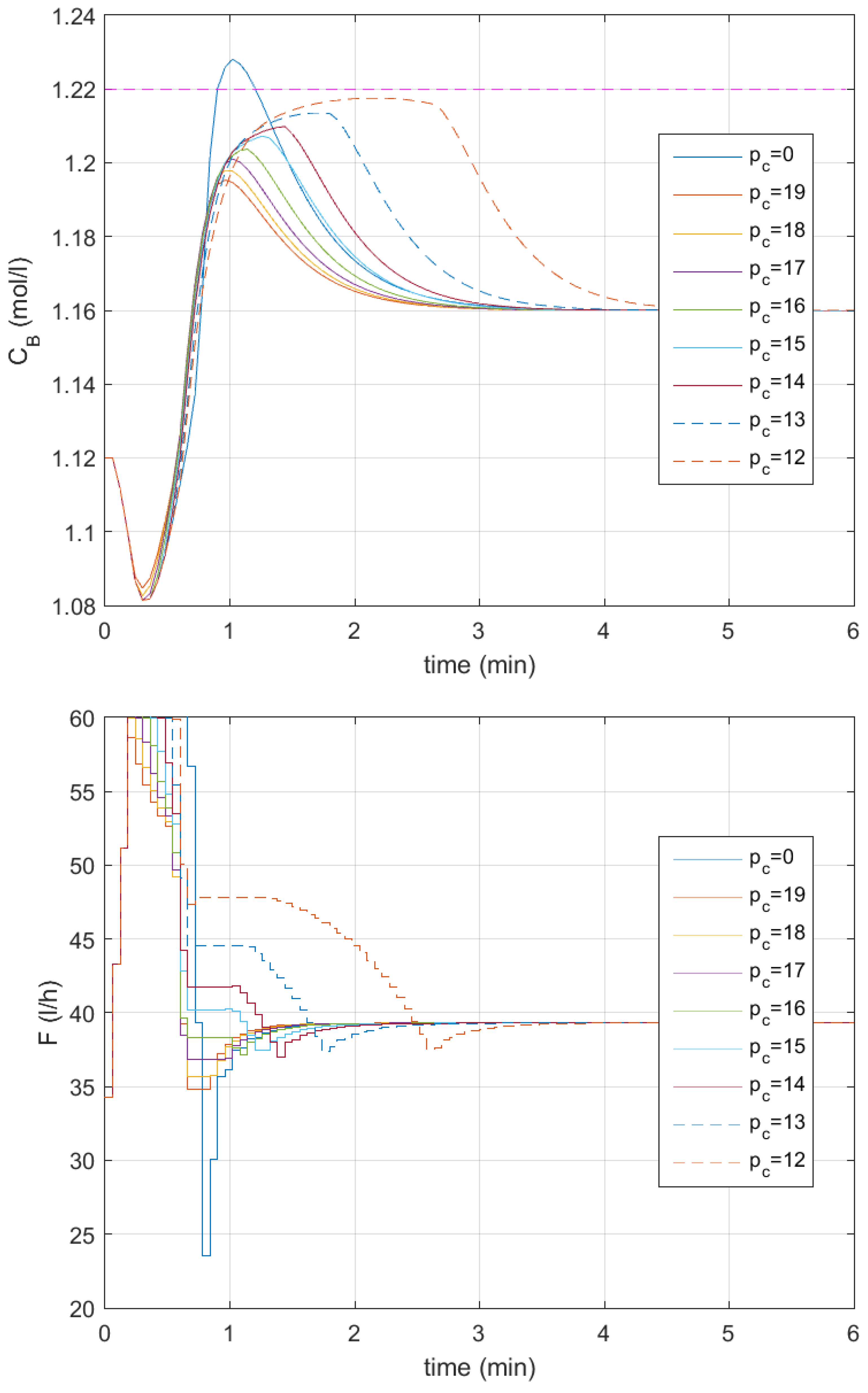
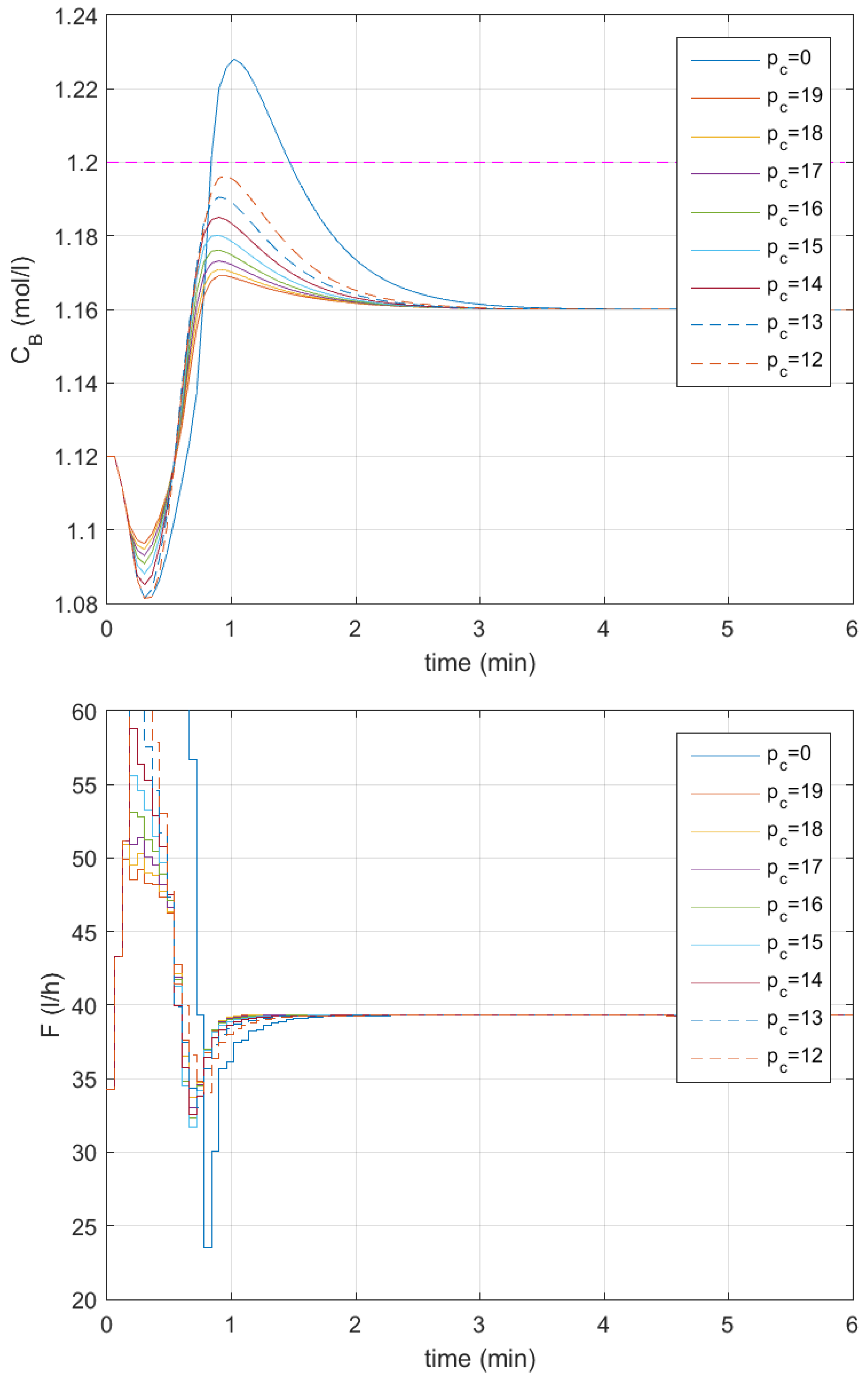
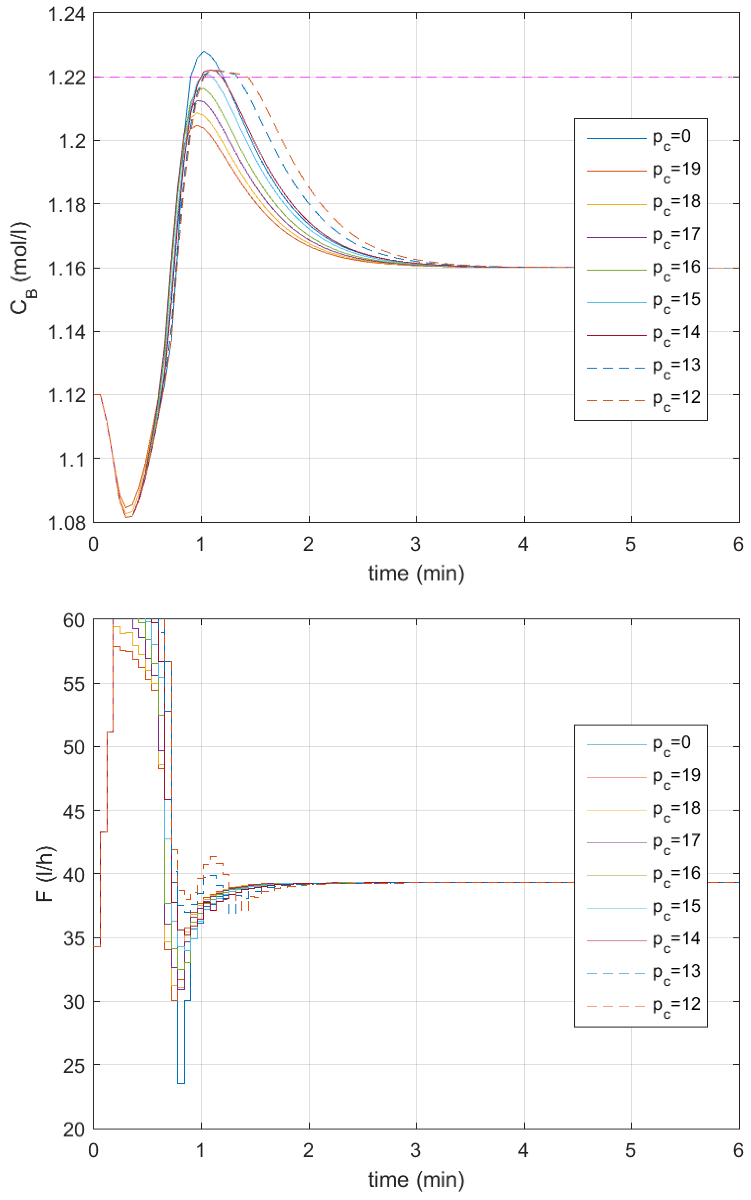
| 19 | Figure 7 red lines | 88.33 | 2.34 | 0.0473 | 1.0907 | 342.0586 | 52.8462 |
| 18 | Figure 7 yellow lines | 94.88 | 2.40 | 0.0503 | 1.1424 | 370.0695 | 53.5927 |
| 17 | Figure 7 lilac lines | 102.59 | 2.46 | 0.0541 | 1.2100 | 375.8552 | 51.4157 |
| 16 | Figure 7 green lines | 109.33 | 2.58 | 0.0595 | 1.3130 | 371.5471 | 50.8686 |
| 15 | Figure 7 cyan lines | 118.14 | 2.76 | 0.0681 | 1.4768 | 347.7047 | 50.3047 |
| 14 | Figure 7 brown lines | 124.61 | 2.94 | 0.0764 | 1.6269 | 339.5394 | 51.1416 |
| 13 | Figure 7 dashed blue lines | 133.77 | 3.36 | 0.0970 | 2.0008 | 307.7444 | 50.4045 |
| 12 | Figure 7 dashed red lines | 143.87 | 4.20 | 0.1451 | 2.8255 | 331.1071 | 50.8947 |
| Response | Overshoot (%) | (min) | SSE | SAE | CE2 | CE1 | |
|---|---|---|---|---|---|---|---|
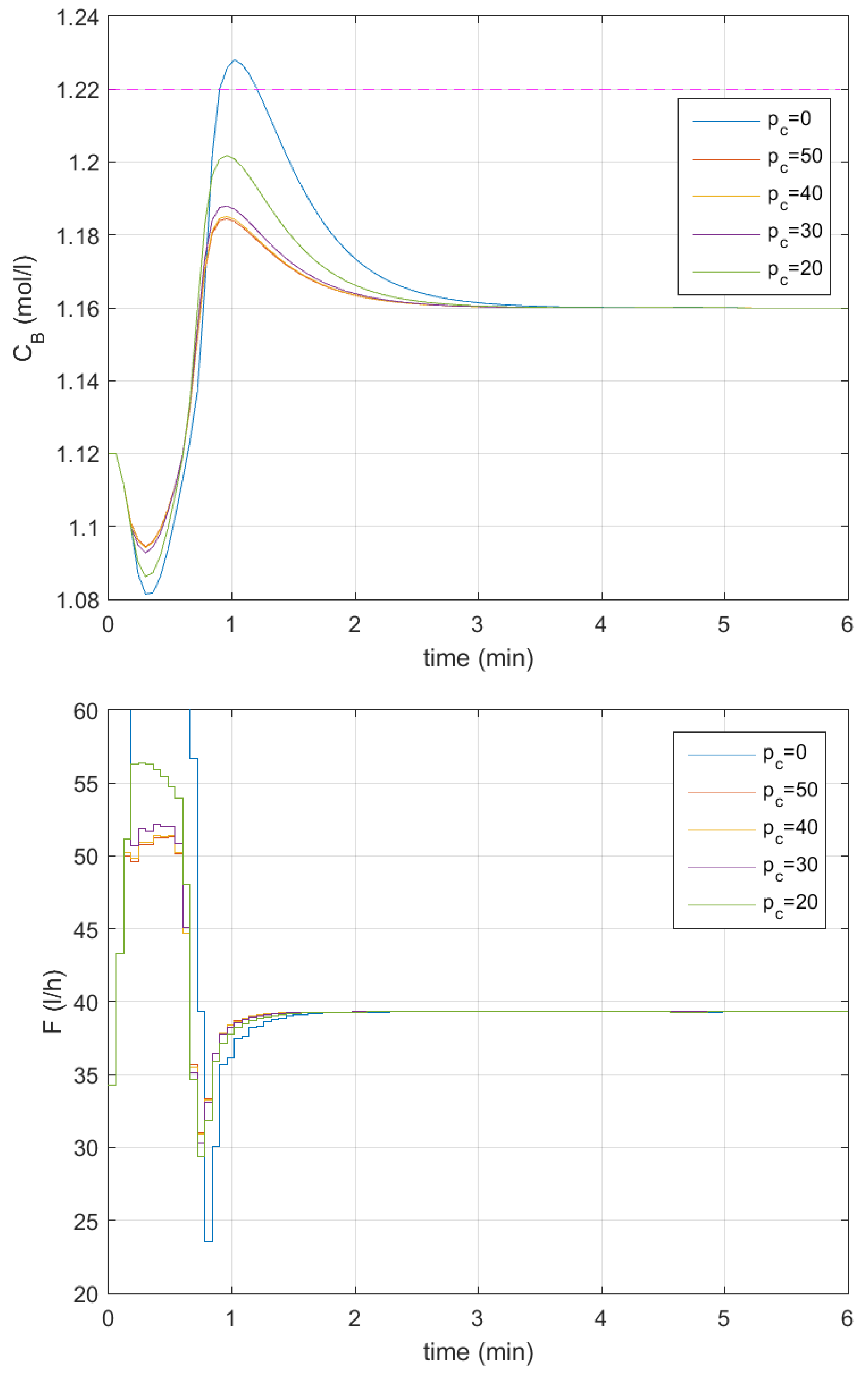
| 0 | Figure 8 blue lines | 170.24 | 2.82 | 0.0869 | 1.6704 | 860.3386 | 78.0063 |
| 50–70 | Figure 8 red lines | 61.10 | 2.22 | 0.0378 | 0.9244 | 278.2876 | 46.2883 |
| 40 | Figure 8 yellow lines | 62.65 | 2.22 | 0.0383 | 0.9332 | 286.3107 | 46.9795 |
| 30 | Figure 8 lilac lines | 69.92 | 2.22 | 0.0403 | 0.9754 | 324.0184 | 50.1329 |
| 20 | Figure 8 green lines | 104.43 | 2.46 | 0.0531 | 1.1946 | 437.9217 | 59.1939 |
| 19 | Figure 9 red lines | 111.95 | 2.46 | 0.0566 | 1.2472 | 467.8681 | 60.6568 |
| 18 | Figure 9 yellow lines | 121.55 | 2.52 | 0.0612 | 1.3155 | 482.7002 | 61.7352 |
| 17 | Figure 9 lilac lines | 131.29 | 2.58 | 0.0665 | 1.3898 | 479.9359 | 63.1520 |
| 16 | Figure 9 green lines | 140.91 | 2.64 | 0.0715 | 1.4623 | 487.9030 | 60.1499 |
| 15 | Figure 9 cyan lines | 152.24 | 2.76 | 0.0780 | 1.5646 | 441.7799 | 57.1858 |
| 14 | Figure 9 brown lines | 155.22 | 2.82 | 0.0827 | 1.6402 | 421.0542 | 56.0484 |
| 13 | Figure 9 dashed blue lines | 155.03 | 2.94 | 0.0914 | 1.7868 | 432.6910 | 57.4629 |
| 12 | Figure 9 dashed red lines | 155.14 | 3.06 | 0.0977 | 1.8908 | 469.6758 | 57.6537 |
| Response | Overshoot (%) | (min) | SSE | SAE | CE2 | CE1 | |
|---|---|---|---|---|---|---|---|
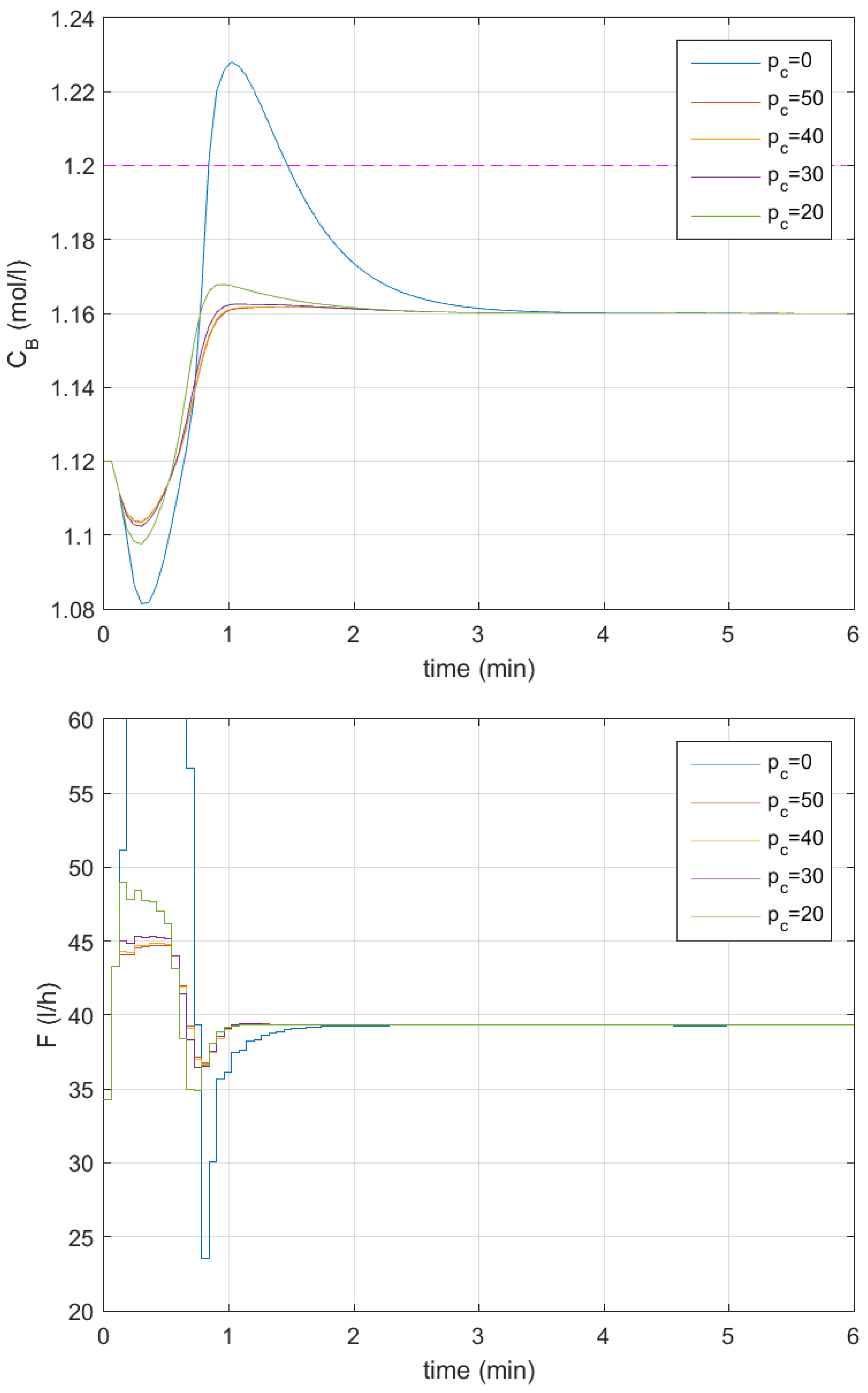
| 0 | Figure 10 blue lines | 170.24 | 2.82 | 0.0869 | 1.6704 | 860.3386 | 78.0063 |
| 50–70 | Figure 10 red lines | 4.46 | 0.90 | 0.0280 | 0.6448 | 100.2492 | 21.2585 |
| 40 | Figure 10 yellow lines | 4.67 | 0.84 | 0.0280 | 0.6451 | 101.4919 | 21.6521 |
| 30 | Figure 10 lilac lines | 6.28 | 1.56 | 0.0282 | 0.6473 | 107.9585 | 23.5195 |
| 20 | Figure 10 green lines | 19.60 | 1.86 | 0.0298 | 0.6851 | 166.6859 | 34.6227 |
| 19 | Figure 11 red lines | 22.76 | 1.86 | 0.0303 | 0.6982 | 185.9079 | 37.5764 |
| 18 | Figure 11 yellow lines | 27.13 | 1.92 | 0.0310 | 0.7141 | 211.8761 | 41.0680 |
| 17 | Figure 11 lilac lines | 32.96 | 1.92 | 0.0322 | 0.7417 | 227.9787 | 42.2610 |
| 16 | Figure 11 green lines | 40.31 | 1.98 | 0.0338 | 0.7824 | 251.7528 | 46.6740 |
| 15 | Figure 11 cyan lines | 50.36 | 2.10 | 0.0363 | 0.8394 | 285.2599 | 52.8949 |
| 14 | Figure 11 brown lines | 62.56 | 2.16 | 0.0397 | 0.9105 | 324.9095 | 57.5839 |
| 13 | Figure 11 dashed blue lines | 76.35 | 2.28 | 0.0442 | 0.9966 | 346.7691 | 59.0407 |
| 12 | Figure 11 dashed red lines | 90.71 | 2.34 | 0.0492 | 1.0972 | 341.1489 | 56.9986 |
| Response | Overshoot (%) | (min) | SSE | SAE | CE2 | CE1 | |
|---|---|---|---|---|---|---|---|
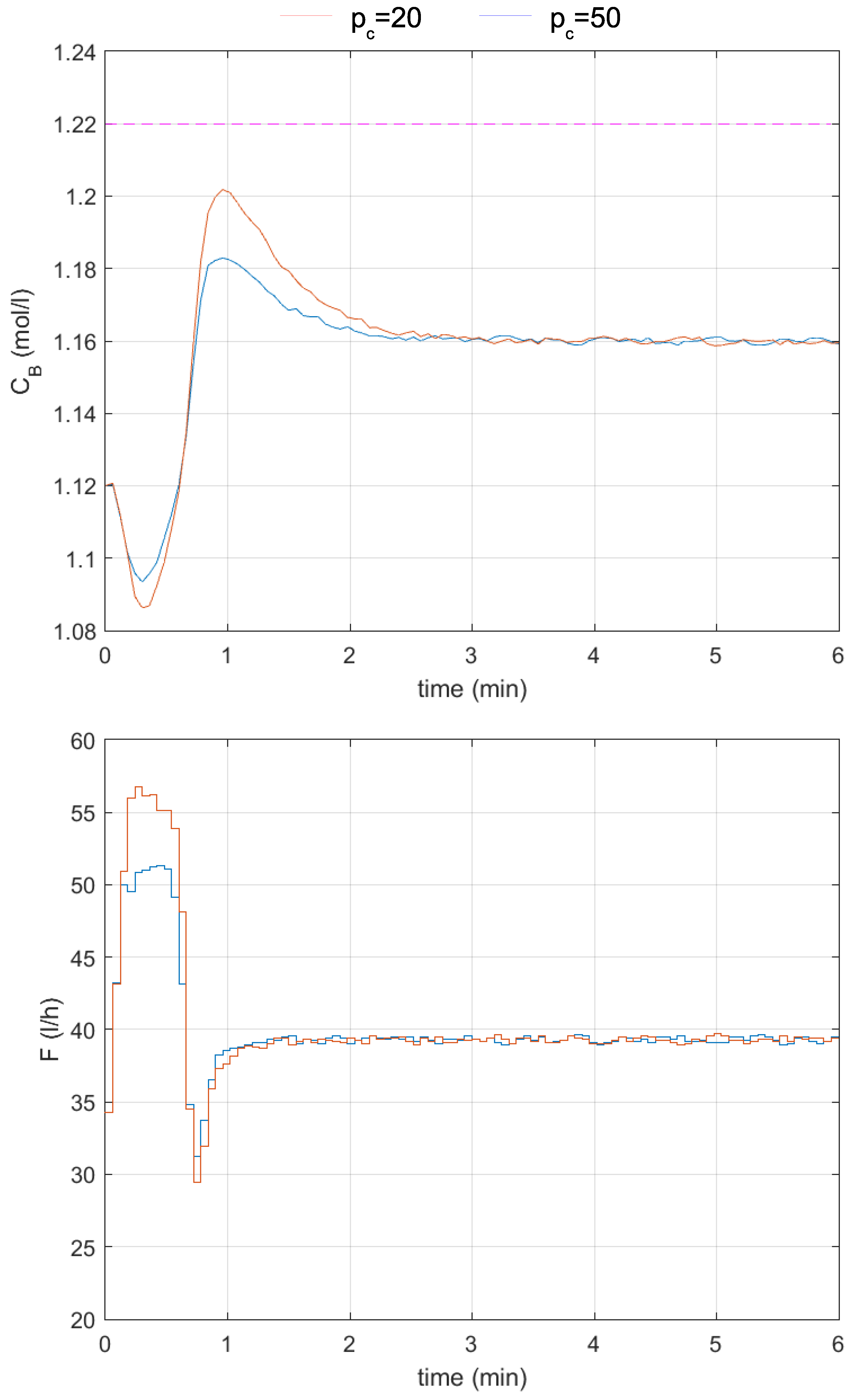
| 50 | Figure 8 red lines no noise | 61.10 | 2.22 | 0.0378 | 0.9244 | 278.2876 | 46.2883 |
| 50 | Figure 12 blue lines with noise | 57.35 | 2.10 | 0.0373 | 0.9289 | 270.7594 | 61.4439 |
| 20 | Figure 8 green lines no noise | 104.43 | 2.46 | 0.0531 | 1.1946 | 437.9217 | 59.1939 |
| 20 | Figure 12 red lines with noise | 104.54 | 2.52 | 0.0529 | 1.2180 | 441.4317 | 74.8157 |
| Response | Overshoot (%) | (min) | SSE | SAE | CE2 | CE1 | |
|---|---|---|---|---|---|---|---|
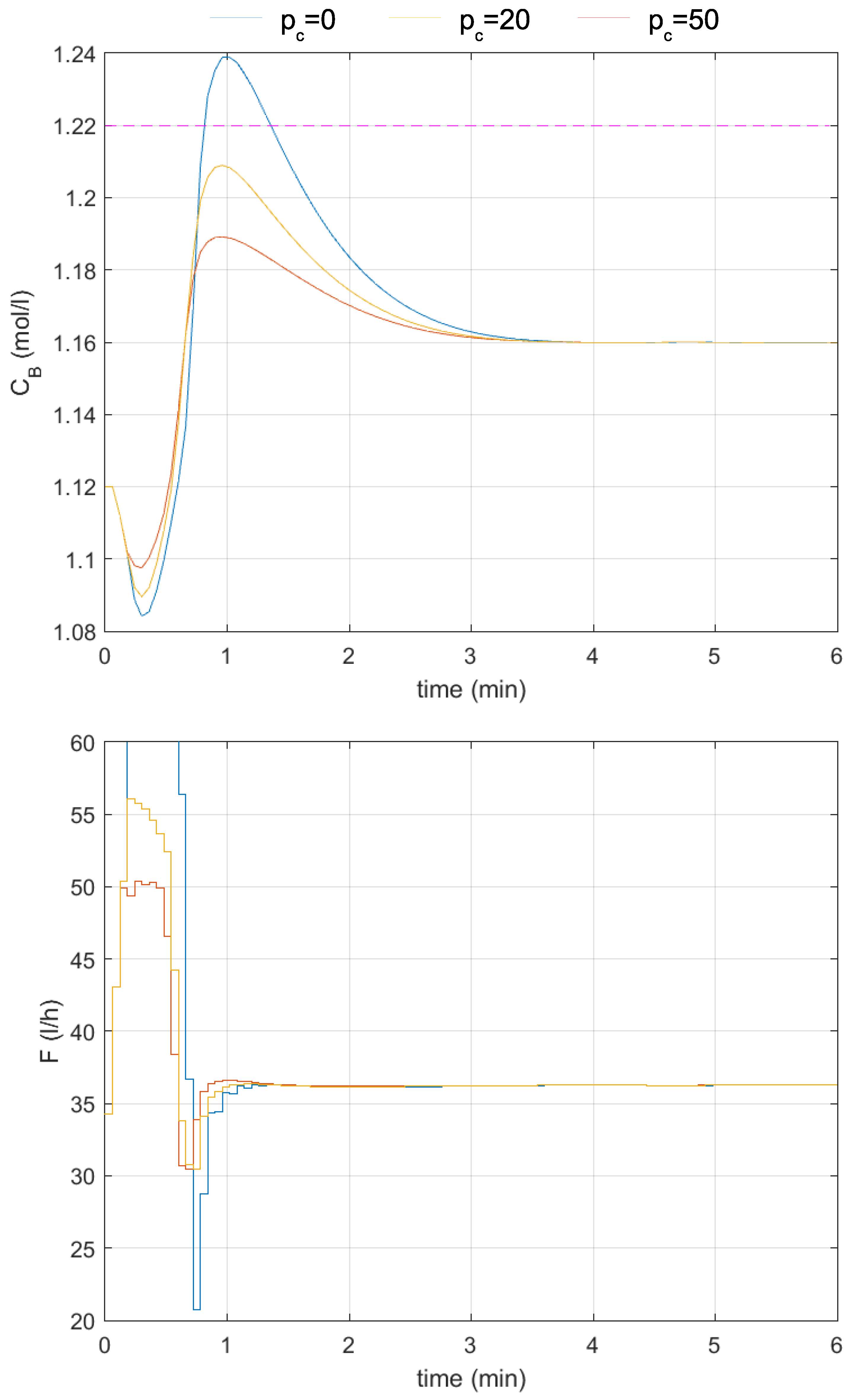
| 0 | Figure 13 blue lines | 197.37 | 3.12 | 0.1097 | 1.9886 | 975.7327 | 81.4058 |
| 50 | Figure 13 red lines | 72.96 | 2.82 | 0.0382 | 1.0789 | 278.0981 | 43.8559 |
| 20 | Figure 13 yellow lines | 122.48 | 2.88 | 0.0599 | 1.4180 | 366.7192 | 53.6553 |
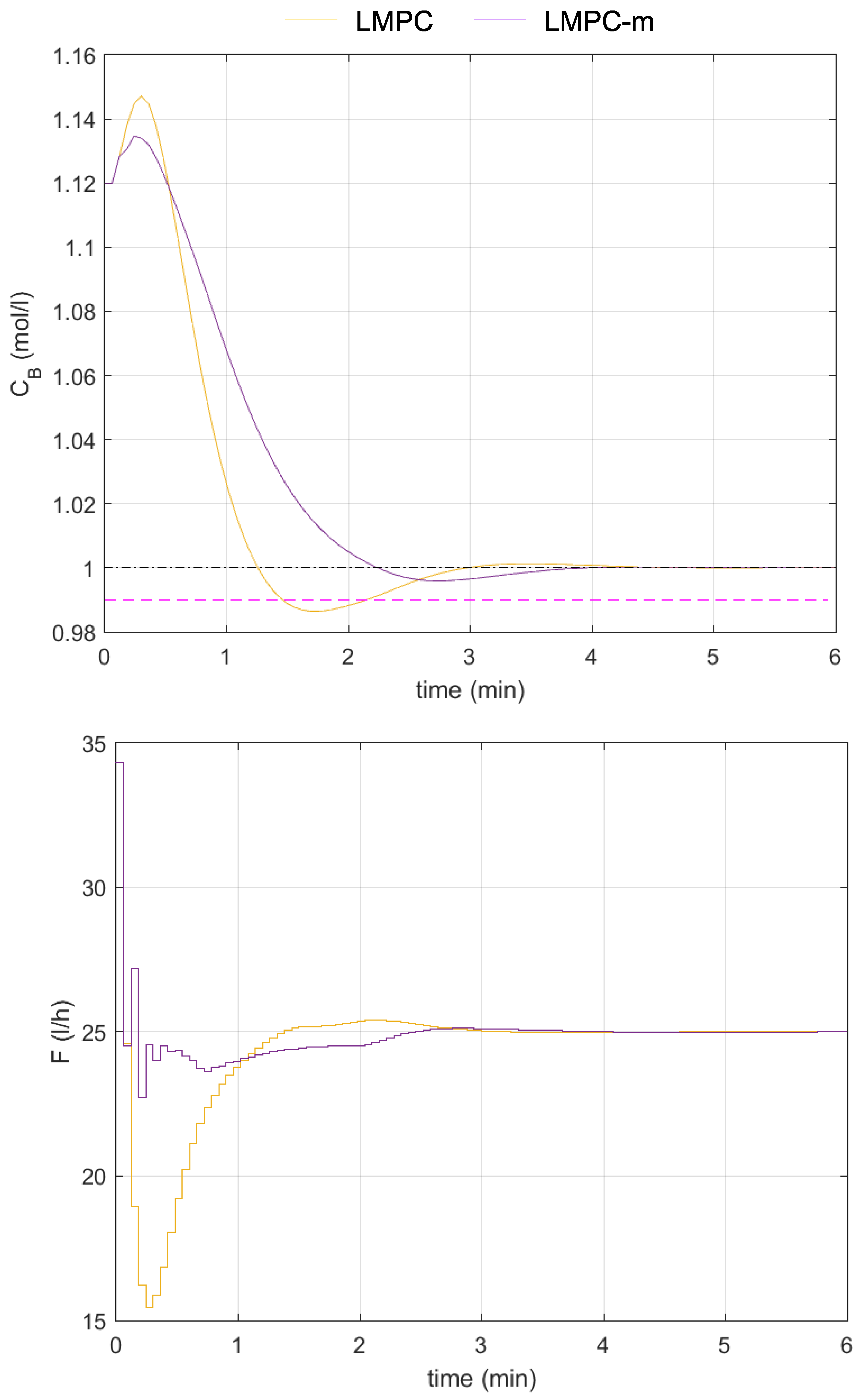
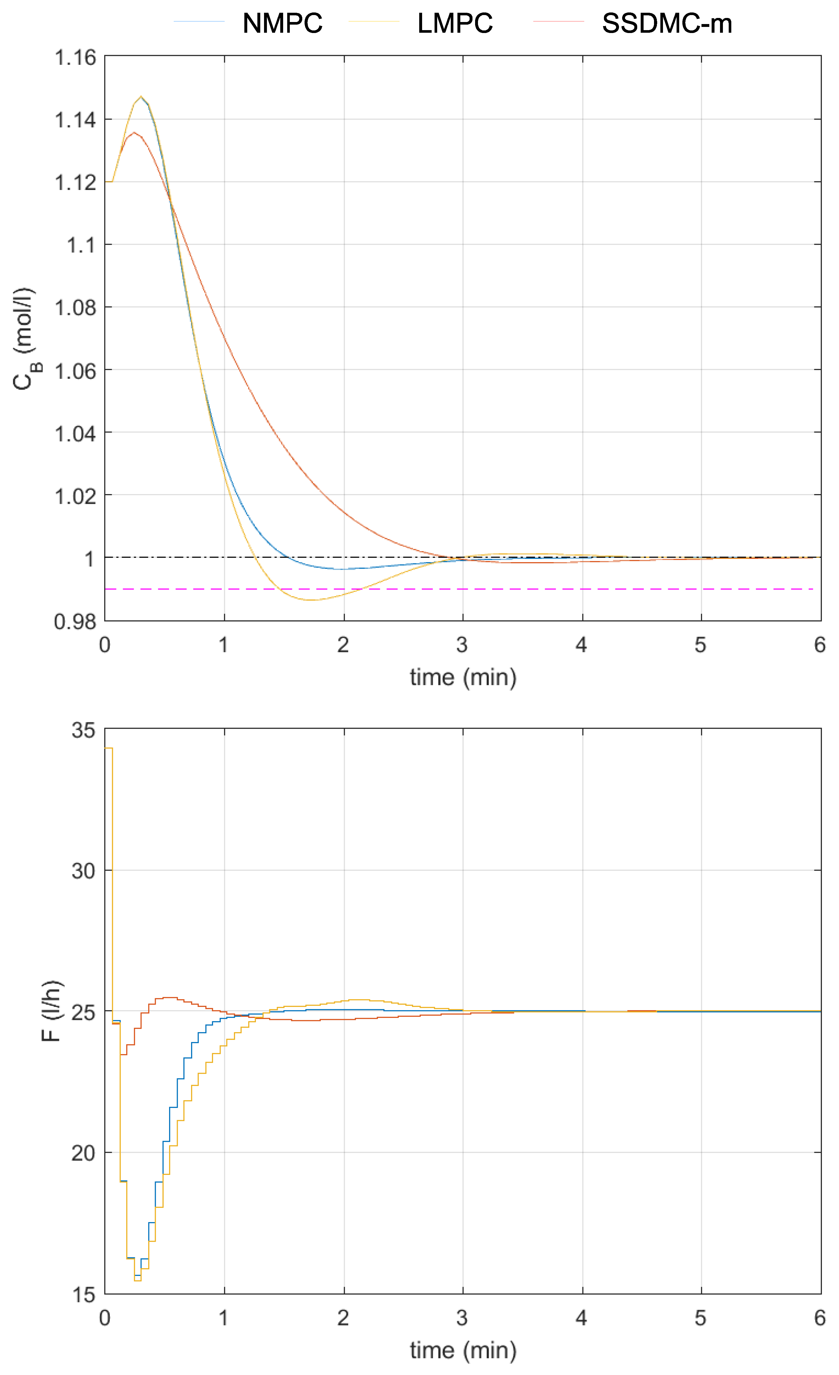
| NMPC–ul | NMPC–l | LMPC–ul | LMPC–l | LMPC–m | SSDMC–m |
|---|---|---|---|---|---|
| 158.5268 | 105.9465 | 5.4905 | 3.8486 | 2.5130 | 0.3305 |
Disclaimer/Publisher’s Note: The statements, opinions and data contained in all publications are solely those of the individual author(s) and contributor(s) and not of MDPI and/or the editor(s). MDPI and/or the editor(s) disclaim responsibility for any injury to people or property resulting from any ideas, methods, instructions or products referred to in the content. |
© 2026 by the authors. Licensee MDPI, Basel, Switzerland. This article is an open access article distributed under the terms and conditions of the Creative Commons Attribution (CC BY) license.
Share and Cite
Marusak, P.; Niewiadomska-Szynkiewicz, E. Fuzzy Model-Based Output Constraint Satisfaction Mechanism for Controllers of Nonlinear Processes. Appl. Sci. 2026, 16, 928. https://doi.org/10.3390/app16020928
Marusak P, Niewiadomska-Szynkiewicz E. Fuzzy Model-Based Output Constraint Satisfaction Mechanism for Controllers of Nonlinear Processes. Applied Sciences. 2026; 16(2):928. https://doi.org/10.3390/app16020928
Chicago/Turabian StyleMarusak, Piotr, and Ewa Niewiadomska-Szynkiewicz. 2026. "Fuzzy Model-Based Output Constraint Satisfaction Mechanism for Controllers of Nonlinear Processes" Applied Sciences 16, no. 2: 928. https://doi.org/10.3390/app16020928
APA StyleMarusak, P., & Niewiadomska-Szynkiewicz, E. (2026). Fuzzy Model-Based Output Constraint Satisfaction Mechanism for Controllers of Nonlinear Processes. Applied Sciences, 16(2), 928. https://doi.org/10.3390/app16020928