Article

Fuzzy Model-Based Output Constraint Satisfaction Mechanism for Controllers of Nonlinear Processes


by
Piotr Marusak
and
Ewa Niewiadomska-Szynkiewicz
*
Institute of Control and Computation Engineering, Faculty of Electronics and Information Technology, Warsaw University of Technology, Nowowiejska 15/19, 00-665 Warszawa, Poland
*
Author to whom correspondence should be addressed.
Appl. Sci. 2026, 16(2), 928; https://doi.org/10.3390/app16020928
Submission received: 26 November 2025 / Revised: 29 December 2025 / Accepted: 14 January 2026 / Published: 16 January 2026
(This article belongs to the Special Issue Enhancing User Experience in Automation and Control Systems)

Abstract

This paper introduces a novel output constraint satisfaction mechanism that can be used to supplement controllers employing a control law. This mechanism is dedicated to control systems of nonlinear processes, with this additional feature. It utilizes an easy-to-obtain fuzzy model composed of step responses, which includes values of the operating points at which these step responses were obtained. The mechanism is based on a prediction approach from Model Predictive Control (MPC) algorithms. Despite this, it can be used with relatively simple controllers (e.g., fuzzy analytical MPC, PID, or Internal Model Control ones). The mechanism involves skillfully modifying the control signal generated by the controller. It is designed in such a way that, under favorable circumstances, the output constraints are not violated, but in less favorable circumstances, the constraint violation can be minimized. The performance and advantages of our mechanism are demonstrated in the simulated control system of an example nonlinear control plant.

1. Introduction

It is crucial to design a control system that provides the best possible performance. The method presented in this article is intended to expand the capabilities of the existing control system, with an important feature of handling output constraints. Output constraints often determine economic efficiency and process security. The method of considering them in a control system can significantly enhance control performance and increase the user’s satisfaction with the control system.
Nowadays, if output constraints are to be taken into consideration, optimization-based control algorithms are usually employed, often MPC ones, e.g., in tracking control, one of the solutions is to employ an MPC algorithm; see, e.g., [1,2]. The alternative to MPC may be the application of reference governors [3]; however, they have important drawbacks, like performance interference with a nominal controller, significant computational demands for complex systems, and dependence on accurate models. They also demand proper tuning and assumptions about system dynamics.
MPC algorithms can be based on nonlinear optimization, referred to as NMPC (Nonlinear MPC) algorithms; see, e.g., [4,5,6,7,8]. In [7,8], suboptimal solutions are accepted to speed the algorithms up. To generate the control signal more quickly and reliably, algorithms based on quadratic optimization have been proposed; see, e.g., [9,10,11]. An interesting group of MPC algorithms are the explicit ones, which fall between numerical and analytical approaches. In the explicit approach, most calculations are performed offline. The algorithms using a nonlinear process model are suboptimal, as seen, e.g., in [12,13,14]. In contrast, those based on the linear model generate optimal solutions [15,16,17]. The main drawback of the explicit approach is that the complexity of the controller grows rapidly with the number of constraints included in the problem. However, in some cases, the available computation capabilities may be limited, and then standard control algorithms based on the control law are used, see, e.g., [18,19]. In such systems, in many cases, taking output constraints into consideration may be desirable due to profits that can be gained, like, e.g., obtaining a higher quality of the product or reducing losses, when a violation of constraints is avoided, and as a result, obtaining economic benefits that increase the satisfaction of the control system user.
We propose and evaluate a novel mechanism for output constraint satisfaction, which can be used to extend existing implementations of standard controllers. Moreover, we introduce two practical methods, namely (i) a method to implement the output constraint satisfaction technique in optimization-based control algorithms and (ii) a method of fuzzy model construction based on expert knowledge exploiting properties of fuzzy modeling. We used fuzzy modeling because it is designed to include expert knowledge in the models relatively easily. Our mechanism of output constraint satisfaction is a simple one. However, unlike the one described in [20], it is designed for control systems of nonlinear plants. The concept of this mechanism is to utilize a skillfully composed fuzzy model. However, we do not propose an alternative method of fuzzy model identification. We propose a technique that supplements the toolbox of the control system designer. Moreover, the method skillfully exploits prediction to formulate constraints in a form that can be easily used, even in algorithms based on the control law. It employs techniques for prediction generation used in MPC algorithms, which enable the inclusion of modeling uncertainty, thereby making the resulting solution more effective. It is worth noting that the main tuning parameter of our output constraint satisfaction mechanism can be utilized to enhance the performance of the control system.
The proposed mechanism is designed to offer good performance with low computational demand, meaning that less computing power is required, resulting in cheaper chips that can be used in embedded systems. Additionally, this approach reduces the likelihood of future problems when chips become scarce and access to them becomes part of the economic rivalry between countries. Moreover, the proposed mechanism can be used relatively easily to modify existing control systems (with control law-based controllers, LMPC, or other MPC algorithms that utilize quadratic optimization) that lack the possibility of output constraint satisfaction or have it based on imprecise linear models.
The article is organized as follows. The next section details how to obtain the model that the proposed mechanism is based on (Section 2.1), how to include output constraints in control systems of standard controllers (Section 2.2), and then how to include information about modeling uncertainty in the proposed mechanism (Section 2.3). In Section 3, the example control system and fuzzy modeling are detailed, the effectiveness of the proposed method is demonstrated in a simulated example control system of a nonlinear chemical reactor with the van de Vusse reaction, a comparison of the proposed approach with standard NMPC and LMPC approaches is also presented and the profits obtained after supplementing the LMPC algorithm with the proposed output constraint satisfaction mechanism are described. The final section presents a summarizing discussion of the obtained results and concludes the article.

2. Materials and Methods

2.1. Obtaining the Fuzzy Process Model

The model used in the mechanism for satisfying output constraints introduced in this paper can be developed using standard optimization-based identification methods or by applying our novel expert knowledge method. It should be emphasized that in our approach, the model can be obtained in a straightforward way. It is, in fact, sufficient to collect step responses near a few operating points and construct a fuzzy model using them. In detail, the procedure used to generate the model is as follows:
1.
The decision regarding the number and location of operating points, near which the responses will be collected, is made. An analysis of the steady-state characteristic may be useful to choose these operating points appropriately. Let us denote the number of the collected responses as l.
2.
The step responses are obtained near each operating point chosen in point no. 1. The coefficients of the step responses are collected until they do not significantly change. Once the changes between the collected coefficients become negligible, obtaining the response is finished. Let p d denote the length of the longest step response. It will be the parameter called the dynamics horizon of the constructed fuzzy model. Thus, in the current step, coefficients a ^ ^ 1 f , , a ^ ^ p d f , f = 1 , , l of step responses are collected, where f is the index of the operating point near which the step response is collected.
3.
From the collected step response coefficients, the output value from which the step response generation started ( y 0 f ) is subtracted:
a ^ i f = a ^ ^ i f y 0 f ( i = 1 , , p d , f = 1 , , l ) .
4.
When collecting the step responses of a nonlinear process, the change in the manipulated variable that can be applied may be different to Δ u = 1 due to the nonlinearity of the process. However, all step responses in the constructed fuzzy model need to be compatible and be responses to the step change by Δ u = 1 in the manipulated variable. Therefore, the responses to changes of other magnitudes than 1 must be scaled. Thus, the following formula is applied to each step response coefficient:
a i f = a ^ i f Δ u f ( i = 1 , , p d , f = 1 , , l ) ,
where Δ u f is the size of the step change in the manipulated variable applied to collect the f th step response.
5.
The collected and scaled step responses are combined to obtain the fuzzy model.
The fuzzy model composed of the aforementioned step responses consists, thus, of the following rules ( f = 1 , , l , l is the number of the collected step responses and, at the same time, the number of local models in the fuzzy TS model of the process):
Rule   f : if x 1 is X 1 f and and x m is X m f then y ^ k f = y 0 f + n = 1 p d 1 a n f · Δ u k n + a p d f · u k p d u 0 f ,
where x 1 , , x m are variables in the antecedents of the fuzzy rules. Most often, they are values of the output variable at the current and previous sampling instants ( y k i , i = 0 , 1 , ) or the manipulated variable at the previous sampling instants ( u k i , i = 1 , 2 , ). X 1 f , , X m f are fuzzy sets, y ^ k f is the output value of the f th local model at the k th sampling instant, Δ u k i are changes in the manipulated variable at the ( k i ) th sampling instant, and u 0 f is the value of the manipulated variable in the f th local model, from which an increase in the manipulated variable was carried out to generate the step response.
The output of the model (3) is described by the following formula:
y ^ k = y ˜ 0 + n = 1 p d 1 a ˜ n · Δ u k n + a ˜ p d · u k p d u ˜ 0 ,
where a ˜ n = f = 1 l w ˜ f · a n f and w ˜ f are the normalized activation levels of the fuzzy rules calculated using fuzzy reasoning, see, e.g., [21,22], y ˜ 0 = f = 1 l w ˜ f · y 0 f and u ˜ 0 = f = 1 l w ˜ f · u 0 f .
Remark 1.
As mentioned, to design the model (3), one can use standard optimization-based identification methods or apply our method based on step responses. In the latter case, the method can be supported by some procedures of fuzzy modeling. To determine the number of local step responses to be collected and their optimal locations, one can utilize the methods developed for fuzzy models (see, e.g., [21]). A review of fuzzy clustering methods can be found, for example, in [23]. However, to avoid problems with the completeness and consistency of the rule base and poor model interpolation in regions between operating points, we propose an iterative expert approach, as illustrated in the example, with its main idea presented below. In many cases, one already has a linear process model from which the step response can be easily obtained. Next, we generate an input trajectory such that the obtained output trajectory covers all values of the output variable we are interested in. During the analysis of the obtained output trajectory, we can decide to add a local model to enhance the model’s operation using the fuzzy approach. The membership functions should be chosen in a way that they cover all values of the process output. Later, we repeat our test for the fuzzy model and assess the modeling quality by analyzing the obtained trajectories and the value of the SSE. In the next step, we add the next local model if needed. The details of this procedure, applied to the example process, are presented in Section 3.2.

2.2. Output Constraint Satisfaction Mechanism

The constraint satisfaction mechanism in controllers exploiting a control law can be taken into consideration by an appropriate modification of manipulated variable value or increment generated by the controller ( u k or Δ u k ; u k = u k 1 + Δ u k ). To consider the constraints on the output variable, a process model is necessary. Let us assume that we will use model (3) to predict the output value p c sampling instants ahead, and p c will be referred to as the constraint horizon. Moreover, we assume that the manipulated variable will not change in the next sampling instants ( u k + i = u k , Δ u k + i = 0 , i = 1 , , p c ). Then, the output of the process model in the next sampling instants will be given by the following formula:
y ^ k + i = y ˜ 0 i + n = i p d 1 a ˜ n i · Δ u k n + i + a ˜ p d i · u k p d u ˜ 0 i ,
where a ˜ n i = f = 1 l w ˜ f i · a n f and w ˜ f i are the normalized activation levels of the fuzzy rules calculated using fuzzy reasoning in future i th sampling instants, y ˜ 0 i = f = 1 l w ˜ f i · y 0 f and u ˜ 0 i = f = 1 l w ˜ f i · u 0 f .
Now, we demand the fulfillment of the following constraints:
y min y ^ k + i y max ,
where y min and y max are lower and upper output limits, respectively. After using (5) in constraint (6) and rearranging the terms in the formula describing the model output in subsequent, future sampling instants (5), we obtain
y min y ˜ 0 i + a ˜ i i · Δ u k + n = i + 1 p d 1 a ˜ n i · Δ u k n + i + a ˜ p d i · u k p d u ˜ 0 i y max .
The lower constraints transformed to the ones put on the current manipulated variable increment are thus as follows:
a ˜ i i · Δ u k y min y ˜ 0 i n = i + 1 p d 1 a ˜ n i · Δ u k n + i a ˜ p d i · u k p d u ˜ 0 i ,
and the upper ones are
a ˜ i i · Δ u k y max y ˜ 0 i n = i + 1 p d 1 a ˜ n i · Δ u k n + i a ˜ p d i · u k p d u ˜ 0 i .
Now, the rules of the manipulated variable increment Δ u k modification can be formulated (it is sufficient to include them in the implementation of the controller).
For lower constraints, we obtain the following:
If a ˜ i i · Δ u k < y min y ˜ 0 i n = i + 1 p d 1 a ˜ n i · Δ u k n + i a ˜ p d i · u k p d u ˜ 0 i , then
Δ u k = y min y ˜ 0 i n = i + 1 p d 1 a ˜ n i · Δ u k n + i a ˜ p d i · u k p d u ˜ 0 i a ˜ i i ;
For upper constraints, we obtain the following:
If a ˜ i i · Δ u k > y max y ˜ 0 i n = i + 1 p d 1 a ˜ n i · Δ u k n + i a ˜ p d i · u k p d u ˜ 0 i , then
Δ u k = y max y ˜ 0 i n = i + 1 p d 1 a ˜ n i · Δ u k n + i a ˜ p d i · u k p d u ˜ 0 i a ˜ i i .
Remark 2.
The formulas above are formulated for the manipulated variable increment Δ u k . If, however, the controller generates a manipulated variable value, then the proposed rules can be easily transformed to the rules of the manipulated variable value u k modification because Δ u k = u k u k 1 . Then, we obtain
For lower constraints,
If a ˜ i i · u k < y min y ˜ 0 i n = i + 1 p d 1 a ˜ n i · Δ u k n + i a ˜ p d i · u k p d u ˜ 0 i + a ˜ i i · u k 1 , then
u k = y min y ˜ 0 i n = i + 1 p d 1 a ˜ n i · Δ u k n + i a ˜ p d i · u k p d u ˜ 0 i + a ˜ i i · u k 1 a ˜ i i ;
For upper constraints,
If a ˜ i i · u k > y max y ˜ 0 i n = i + 1 p d 1 a ˜ n i · Δ u k n + i a ˜ p d i · u k p d u ˜ 0 i + a ˜ i i · u k 1 , then
Δ u k = y max y ˜ 0 i n = i + 1 p d 1 a ˜ n i · Δ u k n + i a ˜ p d i · u k p d u ˜ 0 i + a ˜ i i · u k 1 a ˜ i i .
Remark 3.
It is important to check if the manipulated variable values and increments modified by the proposed mechanism fulfill the constraints on the manipulated variable. If not, then it means that it is impossible to satisfy the output constraints in the current form and it is advisable to relax them.

2.3. Taking Modeling Uncertainty into Account

It may be useful to consider modeling uncertainty in the proposed mechanism. Two approaches on how to carry it out are proposed.
The first approach is adopted from the predictive control algorithms. In these algorithms, at each sampling instant, the difference between the measured output value and the model’s output is calculated and used to improve the prediction; see, e.g., [24]. Namely, the following formula is applied:
d k = y k y ^ k ,
where y k is the process output measurement in the k th sampling instant, and y ^ k is the output of the model (4).
Now, the output of the model (5) in subsequent, future sampling instants is updated using the assessed modeling inaccuracy (14), and (5) becomes
y ^ k + i | k = y ˜ 0 i + n = i p d 1 a ˜ n i · Δ u k n + i + a ˜ p d i · u k p d u ˜ 0 i + d k ,
Now, we demand the fulfillment of the following constraints:
y min y ^ k + i | k y max .
After applying the same reasoning as before, the following rules of the manipulated variable increment Δ u k modification are formulated.
For lower constraints, we obtain the following:
If a ˜ i i · Δ u k < y min y ˜ 0 i n = i + 1 p d 1 a ˜ n i · Δ u k n + i a ˜ p d i · u k p d u ˜ 0 i d k , then
Δ u k = y min y ˜ 0 i n = i + 1 p d 1 a ˜ n i · Δ u k n + i a ˜ p d i · u k p d u ˜ 0 i d k a ˜ i i ;
For upper constraints, we obtain the following:
If a ˜ i i · Δ u k > y max y ˜ 0 i n = i + 1 p d 1 a ˜ n i · Δ u k n + i a ˜ p d i · u k p d u ˜ 0 i d k , then
Δ u k = y max y ˜ 0 i n = i + 1 p d 1 a ˜ n i · Δ u k n + i a ˜ p d i · u k p d u ˜ 0 i d k a ˜ i i .
The second approach to include information about modeling inaccuracy in the proposed mechanism is based on the assumption that it can be assessed. If so, let us assume that modeling inaccuracy influences the prediction of future output values:
y ^ k + i | k = y ˜ 0 i + n = i p d 1 a ˜ n i · Δ u k n + i + a ˜ p d i · u k p d u ˜ 0 i + v k + i ,
where v k + i represents modeling inaccuracy, which is usually not known precisely, but it can often be assessed. Thus, assume that it is bounded:
v k + i min v k + i v k + i max ,
where v k + i min 0 and v k + i max 0 are minimum and maximum assessments of inaccuracy v k + i , respectively. Therefore, applying the same reasoning as in the previous considerations leads to the following rules of the manipulated variable increment Δ u k modification:
For lower constraints,
If a ˜ i i · Δ u k < y min y ˜ 0 i n = i + 1 p d 1 a ˜ n i · Δ u k n + i a ˜ p d i · u k p d u ˜ 0 i v k + i min , then
Δ u k = y min y ˜ 0 i n = i + 1 p d 1 a ˜ n i · Δ u k n + i a ˜ p d i · u k p d u ˜ 0 i v k + i min a ˜ i i ;
For upper constraints,
If a ˜ i i · Δ u k > y max y ˜ 0 i n = i + 1 p d 1 a ˜ n i · Δ u k n + i a ˜ p d i · u k p d u ˜ 0 i v k + i max , then
Δ u k = y max y ˜ 0 i n = i + 1 p d 1 a ˜ n i · Δ u k n + i a ˜ p d i · u k p d u ˜ 0 i v k + i max a ˜ i i .
Remark 4.
The output constraints detailed in the current section should now be included in the standard mechanism of control projection on the constraint set used in the analytical MPC algorithm (see, e.g., [24] for details). However, it is essential to consider constraints in the correct order. That is, first, the constraints on the output variable as detailed in the current section. The control increment or the control value after modification applied at this stage may exceed the limits of the control signal. To avoid feasibility problems, constraints on the control signal should be applied after constraints on the output variable have been applied. If the control signal constraints enforce the modification of the control increment at this stage, it means the output constraints cannot be fulfilled.
Remark 5.
Note that constraints (8) and (9) are linear with respect to the decision variable, Δ u k . Therefore (after supplementing them with the mechanism of taking modeling uncertainty into account), they can be used to improve the operation of the LMPC algorithm if such an algorithm has already been implemented. This is because the prediction using the fuzzy model is more accurate in cases involving nonlinear processes than the one based on a linear model. Therefore, the operation of standard approaches based on quadratic programming, such as LMPC, can be relatively easily improved by employing the proposed mechanism. Actually, in the case of reference governors based on solving linear or quadratic programming problems, the mentioned constraints can also be relatively easily incorporated into the optimization problems, thereby increasing the capabilities of these governors.

3. Results

3.1. Example Control System

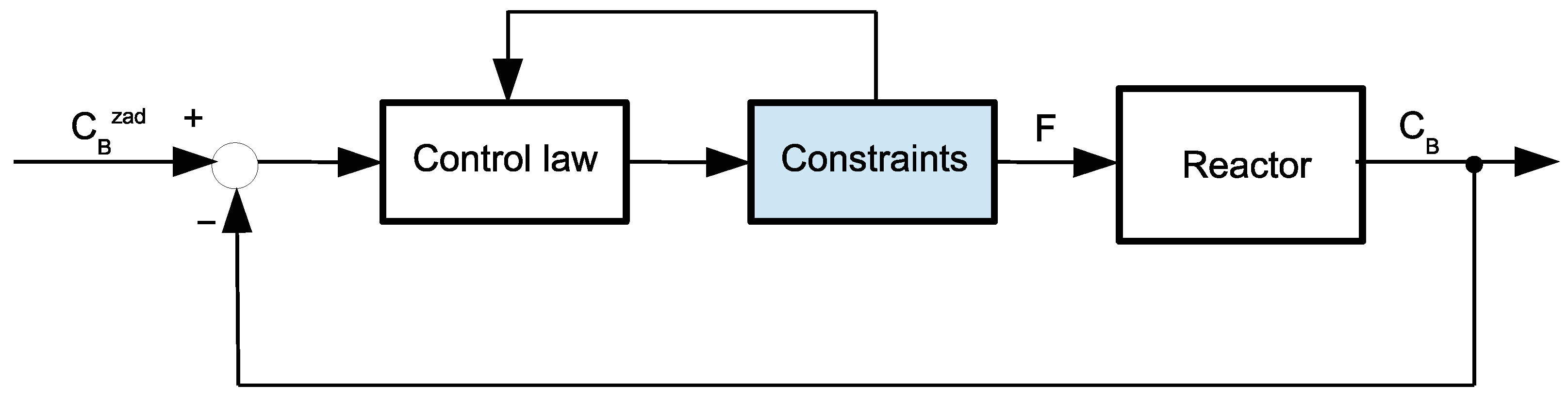
The effectiveness of the proposed output constraint satisfaction mechanism was tested in the control system of a nonlinear, isothermal chemical reactor, where the van de Vusse reaction took place, with the controller detailed in [25]. The structure of the control system is depicted in Figure 1. The control system was simulated in Matlab on the PC equipped with the AMD Athlon II X3 460 processor running at 3.40 GHz. A sampling time equal to T s = 3.6 s was assumed.
The control plant is not only nonlinear but also is non-minimum phase. Therefore, it is difficult to control using standard control algorithms and is willingly used as a benchmark to test advanced control algorithms. A recent review of control methods for reactors with the van de Vusse reaction can be found in [26]. A comparison of the PID controller designed in [27], which is considered the best one, with an MPC-type controller can be found in [28].The output variable of the reactor is the concentration, C B , of substance B in the reactor, and the control signal is the flow rate, F, through the reactor. It is assumed that the control signal is constrained and its lower bound is equal to F m i n = 0 L / h . The upper bound is equal to F m a x = 60 L / h . The model of the reactor is as follows [29]:
d C A d t = k 1 · C A k 3 · C A 2 + F V C Af C A , d C B d t = k 1 · C A k 2 · C B F V C B ,
where C A —the concentration of component A, V—the volume in which the reaction takes place (assumed constant and V = 1 L ), and C Af —the concentration of component A in the inlet flow stream is the disturbance variable ( C Af = 10 mol / L if not declared otherwise). The parameters of the model have the following values: k 1 = 50 1 / h , k 2 = 100 1 / h , and k 3 = 10 L / ( h · mol ) .
The employed controller is the SSDMC controller proposed in [25]. Its control law is as follows:
Δ u k = r 0 , k · e k + i = 1 p d 1 r i · Δ u k i ,
where r 0 , k = 1 K k · r 0 and r 0 , r 1 , , r p d are derived in the same way as in the control law of the standard analytical DMC algorithm, using the red normalized step response from Figure 2 (see, e.g., in [24]), K k is the gain of the control plant in the current operating point (the details are given in [25]). The controller was detuned to obtain responses with significant overshoot. Thus, the assumed parameters of the controller are as follows: prediction horizon p = 70 , control horizon s = 2 , and coefficient λ = 10 5 .
The crucial block in the control system is the one called “Constraints”. It is the block that is present in control systems with analytical predictive controllers and implements control projection on a constraint set to consider control signal constraints (for details, see, e.g., [24]). The block from Figure 1 was appropriately modified (extended with the capability to take output constraints into consideration, as described in Remark 4 from Section 2). It is assumed that it performs all the tasks needed for its operation. Namely, it obtains control increments generated using the control law of the control algorithm, then it considers the constraints by an appropriate modification of control increments, and finally adds the modified control increment to the last control value, u k 1 , to obtain the current control value, u k , sent to the control plant. The control increments after modification must then be returned to the control law of the control algorithm (the control algorithm must have information about the control increments that have been actually sent to the control plant).

3.2. Obtaining Simplified Process Model

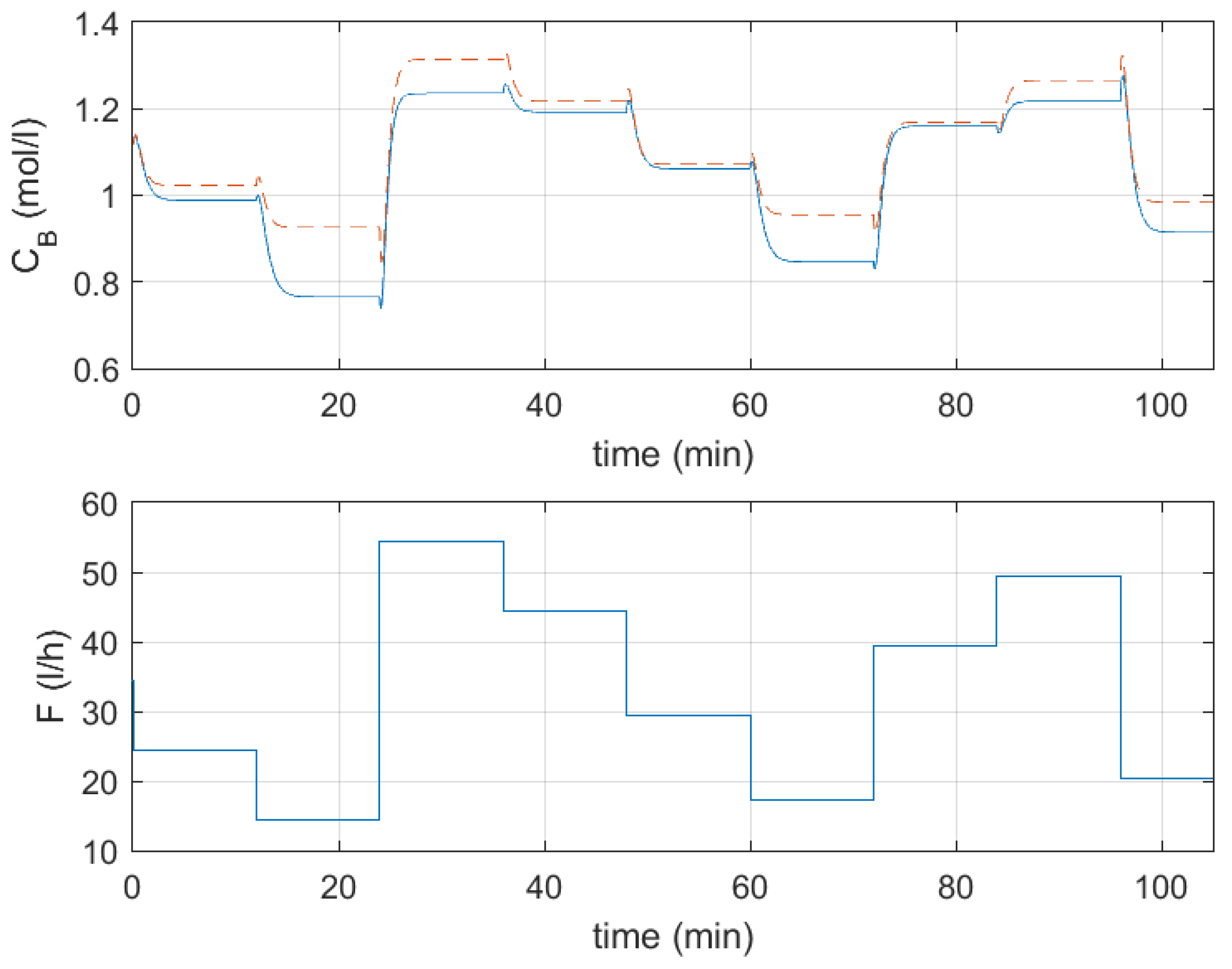
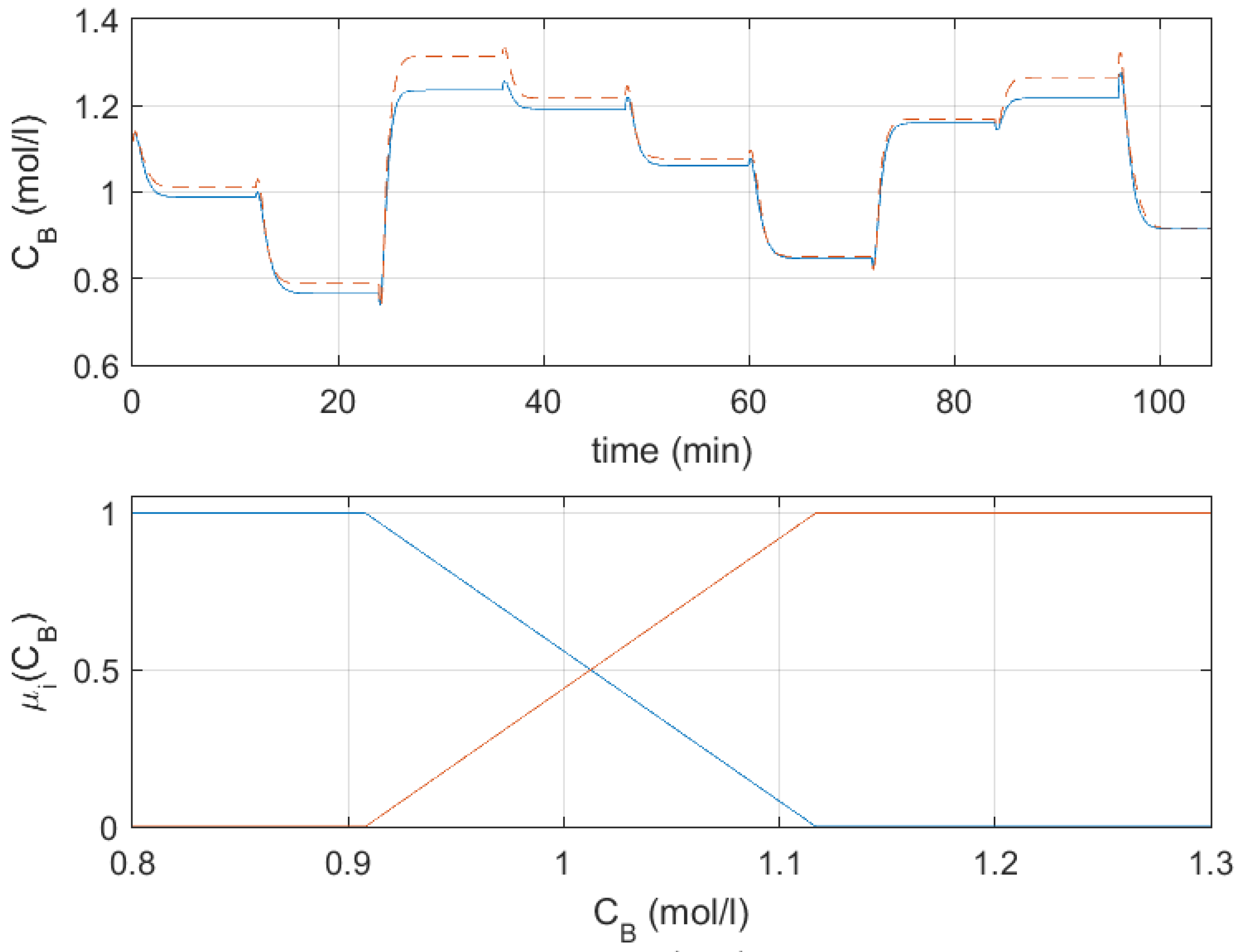
The iterative procedure for obtaining the simplified process model was applied. It started with a single step response (a linear model) obtained for medium values of the process output, C B . In many cases, a linear model is already available, and obtaining its step response is not a problem if needed. The output trajectories obtained using the original model and the linear model are depicted at the top of Figure 3, the input trajectory is shown at the bottom of Figure 3, and the SSE calculated using differences between outputs of the models is equal to 9.3097 (values of the SSE obtained for different models are collected in Table 1). As expected, the model works well in the medium range of output values but generates significant errors elsewhere, especially for small values of the output variable. Therefore, in the next identification step, the fuzzy model composed of two local models was developed, with an additional local model obtained for small output variable values. The obtained SSE is more than 4 times smaller for this model, and the modeling quality for small values of the output variable visibly improves (the top of Figure 4). The assumed membership functions are depicted in the bottom part of Figure 4. Note that their shape is such that they cover all values of the output variable.
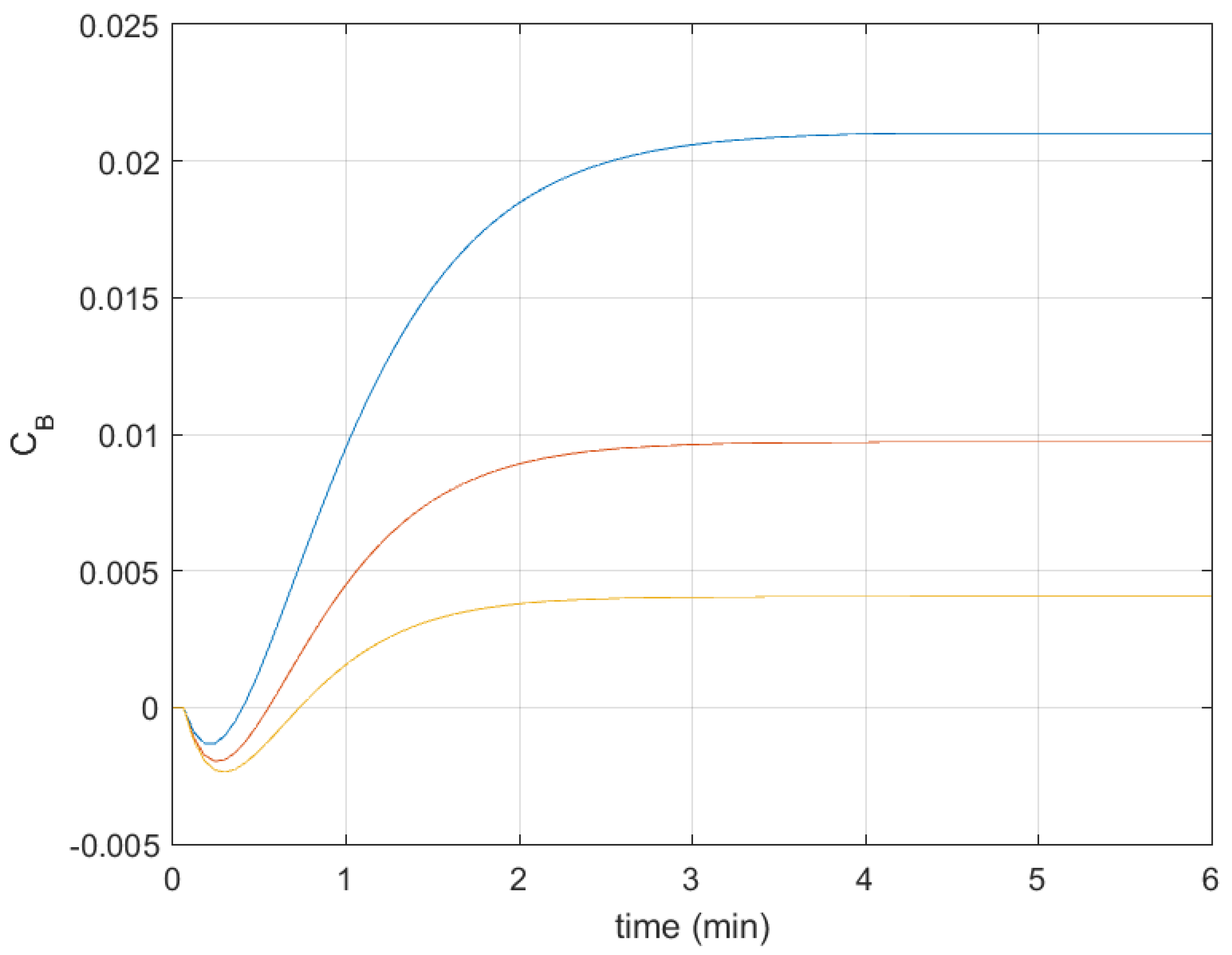
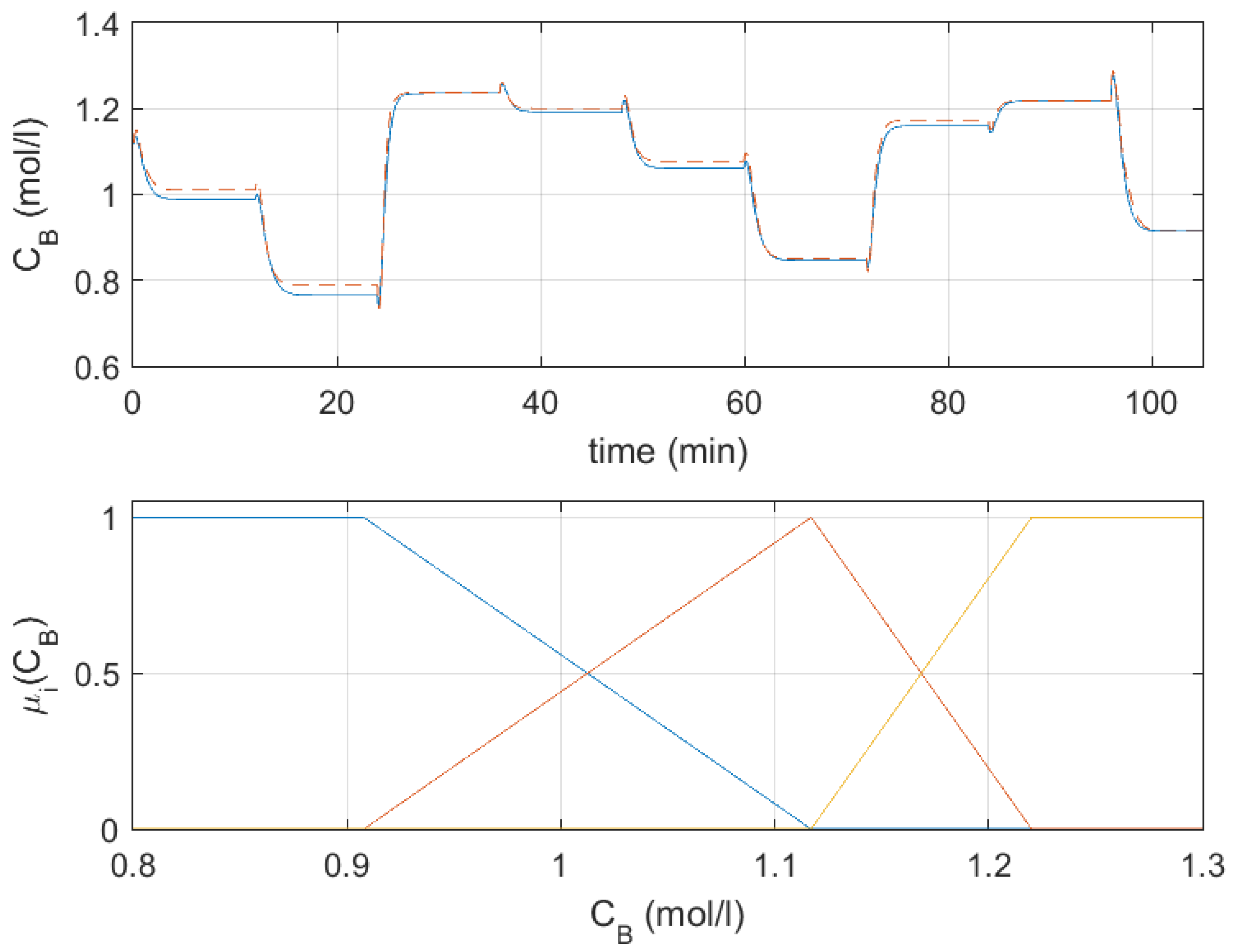
When analyzing the output trajectories in Figure 4, it is clear that modeling quality can be improved for large values of the output variable. Therefore, the third local model was added to the fuzzy model. The assumed membership functions are depicted in the bottom part of Figure 5 (they still cover all values of the output variable). The model now also works well for large output values (the top part of Figure 5 shows a comparison of trajectories generated by the original and the fuzzy models). The SSE is more than 5.5 times better than that of the fuzzy model composed of two local models. Thus, this model (consisting of three local models) is our target fuzzy model, used later in the proposed output constraint satisfaction mechanism. The normalized responses of the fuzzy model are depicted in Figure 2. They are drawn with colors corresponding to the colors of membership functions shown in Figure 4 and Figure 5. The values of y 0 f and u 0 f parameters are summarized in Table 2.

3.3. Experiments

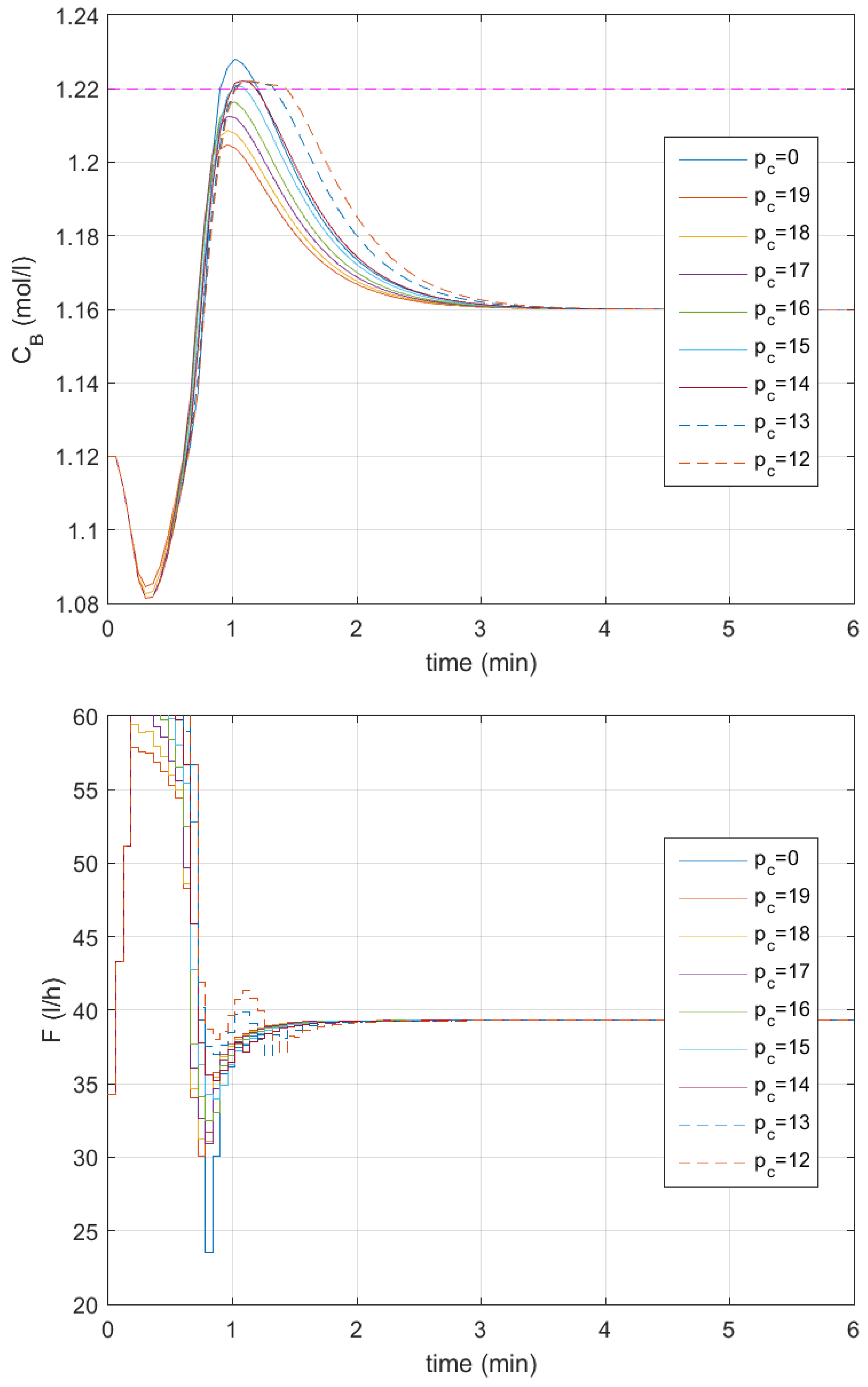
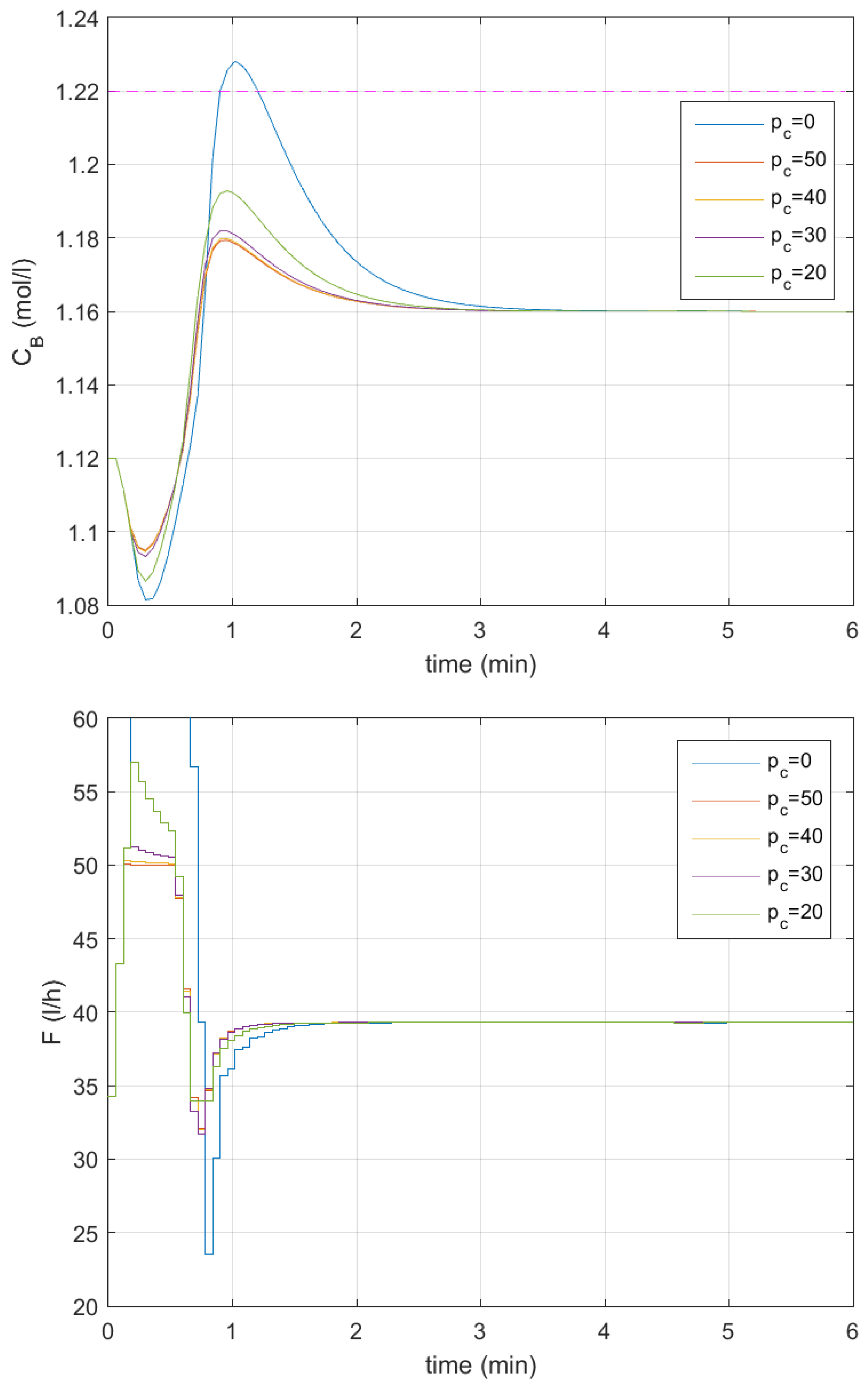
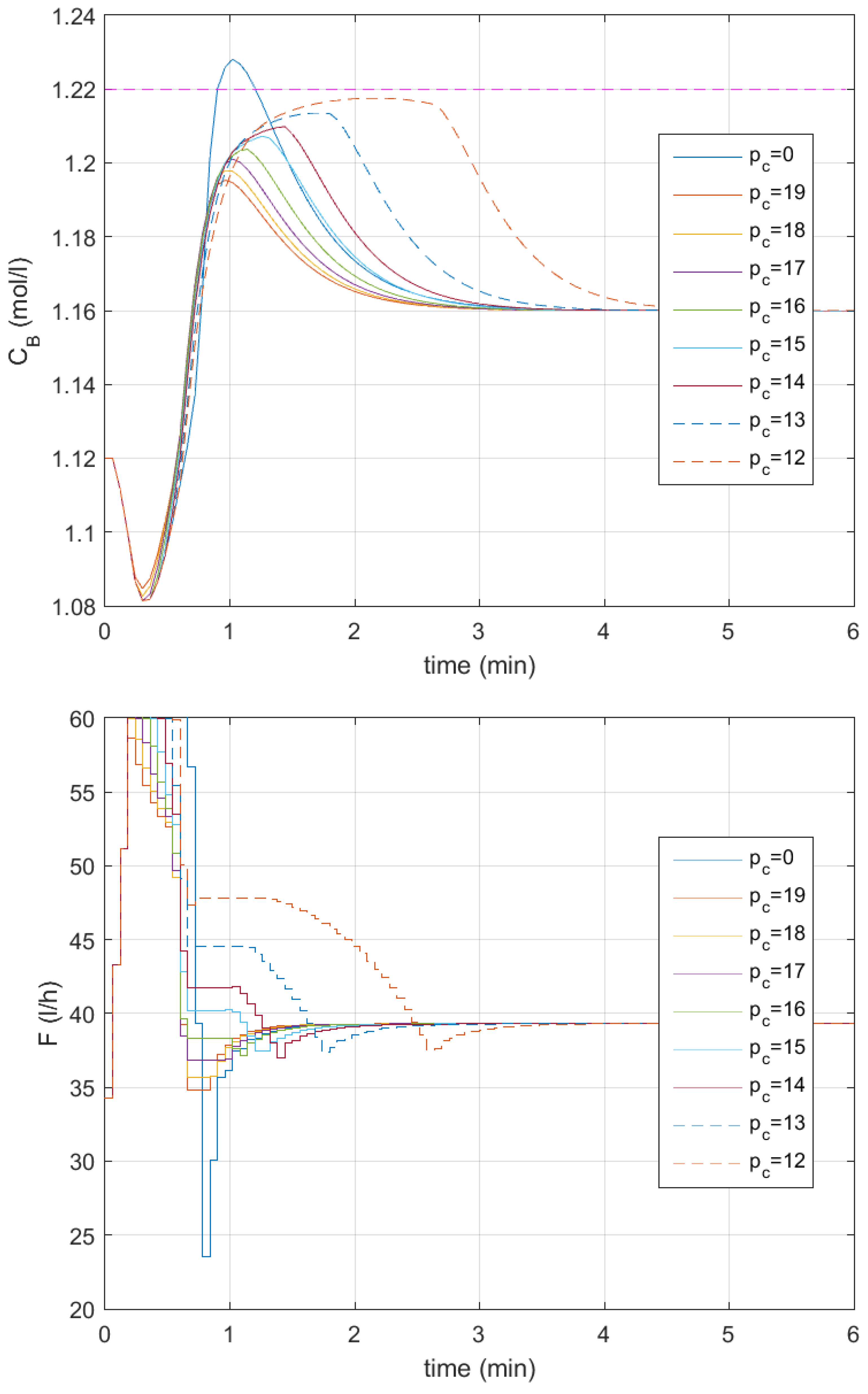
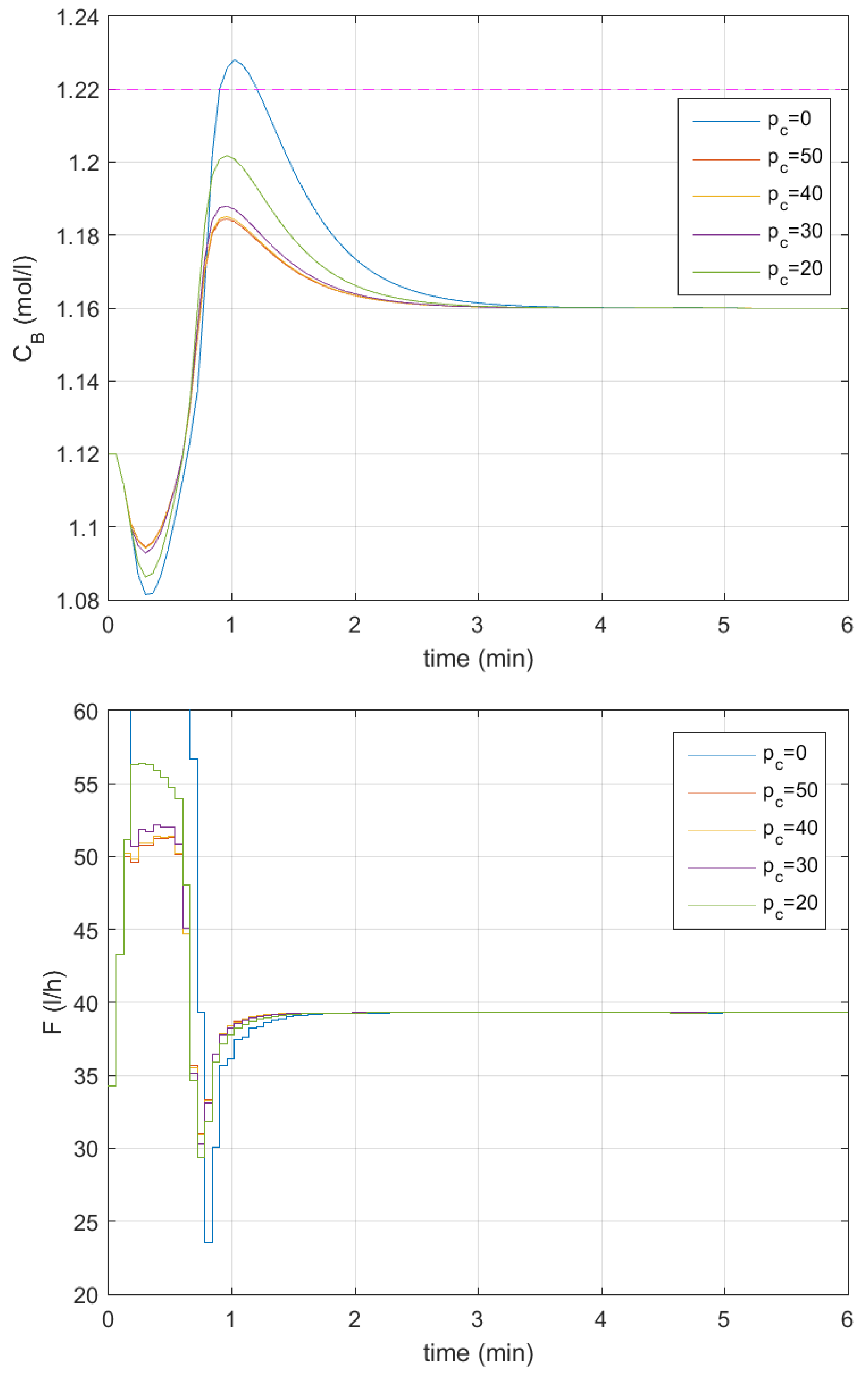
First, the basic version of the output constraint satisfaction mechanism relying only on the process model, without the inclusion of modeling uncertainty, was tested for different values of the constraint horizon (Figure 6 and Figure 7). It was assumed that the setpoint is equal to C ¯ B 1 = 1.16 mol/L and that the upper output constraint is set on C B , m a x = 1.22 mol/L. Different constraint horizon values were tested. The control quality indicators, like overshoot, settling time t s , SSE, SAE, and control effort indicators
C E 1 = n = 1 h s i m | Δ u k + n | ,
where h s i m is the number of time steps of the simulation experiment (the horizon of the simulation) and
C E 2 = n = 1 h s i m Δ u k + n 2
are been calculated and presented in Table 3.
In the reference responses, when no output constraint satisfaction mechanism is employed (drawn with blue lines in all subsequent figures), the constraint is violated. When constraint horizon p c [ 50 , 70 ] is assumed, the output response is far from the constraint, and the overshoot caused by the detuning of the controller is reduced from 170 % to 48 % . The settling time is reduced from t s = 2.82 min to t s = 2.1 min, the SSE is reduced more than 2 times, the SAE is reduced around 2 times, the quadratic control effort indicator CE2 is reduced more than 3 times, and the CE1 indicator is reduced almost 2 times. For constraint horizon p c = 40 , the responses change only slightly compared to the previous case. When the constraint horizon is set to p c = 30 , the difference in responses becomes visible. However, we can observe that for a significant set of constraint horizon values, the obtained responses are similar. When the constraint horizon is decreased even more, to p c = 20 , the maximal value of the output signal more closely approaches the constraint as the overshoot grows to 82 % , and the settling time also increases to t s = 2.34 min. However, it is still smaller than in the case where the proposed mechanism is not used. The other indicators (SSE, SAE, and control effort indicators) also increase but are still significantly smaller than in the reference case.
In further experiments, the constraint horizon decreases even more (Figure 7). When the constraint horizon gradually decreases, the overshoot, settling time, SSE, and SAE grow, but the control effort indicators do not manifest this tendency. The CE2 indicator achieves a local maximum for constraint horizon p c = 17 and the CE1 indicator achieves it for constraint horizon p c = 18 . For constraint horizon p c = 15 , the maximum of the output response begins to become longer, and the settling time stretches out to t s = 2.76 min (almost equal to the value obtained for the reference response— t s = 2.82 min). This problem becomes particularly severe when the constraint horizon is shortened even further. For p c = 14 , the settling time t s = 2.94 min is slightly longer than in the reference case. Unfortunately, with a further decrease in the constraint horizon, the settling time deteriorates rapidly. For p c = 13 , it is t s = 3.36 min, and for p c = 12 , it is t s = 4.2 min. In the latter two cases, the obtained settling times are unacceptably long, and the responses clearly deteriorate. However, in all cases, the output constraint is not violated. Further decreasing the constraint horizon leads to a deterioration in the controller’s operation. Thus, it becomes clear that modeling uncertainty should be taken into consideration in the proposed mechanism.
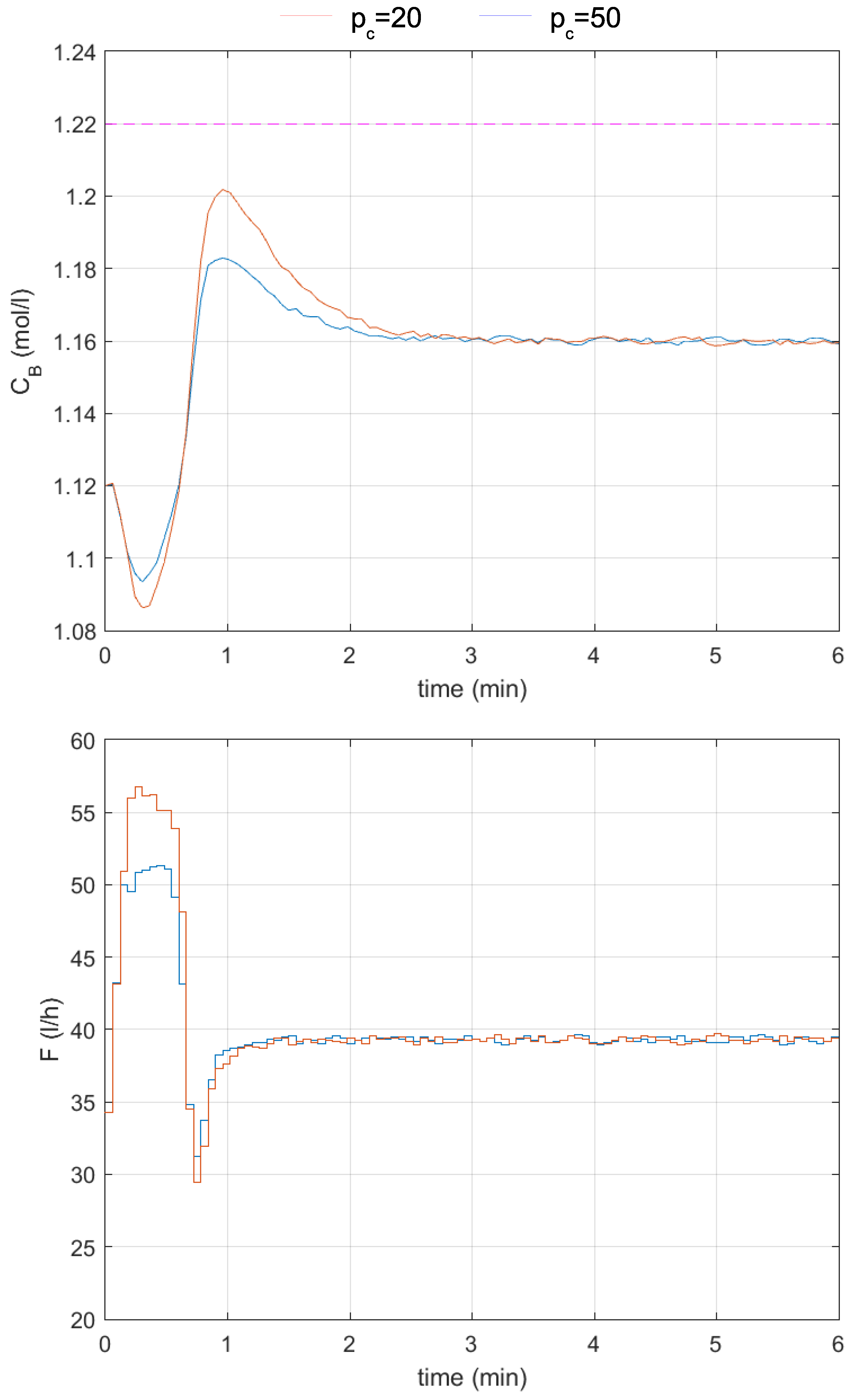
Next, the first variant of the modeling inaccuracy assessment is employed (Figure 8 and Figure 9). Table 4 contains values of the obtained control quality indicators. The tendencies observed when changing the constraint horizon between 70 and 20 are the same as before (Figure 8). Namely, for constraint horizon p c [ 50 , 70 ] , the output response is far from the constraint, the overshoot caused by the detuning of the controller is reduced to 61 % , the settling time is reduced to t s = 2.22 min, the SSE and CE2 indicators decrease more than 2 times, and the SAE and CE1 indicators decrease more than 1.5 times compared to the reference case. For constraint horizons p c = 40 and p c = 30 , the responses change only slightly, and the obtained responses are similar. The settling time remains practically unchanged, while the other control quality indicators increase gradually as the constraint horizon decreases. A bigger difference in responses occurs when the constraint horizon is set to p c = 20 ; the maximal value of the output signal is visibly closer to the constraint than in the previous case because the overshoot increases to 104 % and the settling time rises to t s = 2.46 min, and the increment of other indicators is now much bigger than in the case of previously applied changes to the constraint horizon.
When the constraint horizon is further decreased, the overshoot, settling time, SSE, and SAE gradually grow, as in the previous experiment, whereas the control effort indicator CE2, this time, achieves a local maximum for constraint horizon p c = 16 , and the CE1 indicator achieves it for constraint horizon p c = 17 . When the constraint horizon is set between p c = 19 and p c = 14 , the shape of the obtained responses is similar to that obtained so far. The same happens when the constraint horizon is decreased even further to p c = 13 and p c = 12 . This time, the obtained responses are visibly different to those in the previous case, where modeling uncertainty was taken into consideration (Figure 9). However, the obtained responses do not deteriorate as much as in the previous case. The control time is still acceptable—for p c = 13 , it is equal to t s = 2.94 min, and for p c = 12 , it is equal to t s = 3.06 min. Unfortunately, the output constraint is slightly violated for constraint horizon values between p c = 15 and p c = 12 due to the remaining modeling errors. Further decreasing the constraint horizon to p c = 11 leads to us obtaining the same responses as in the case where p c = 12 is set. The obtained results indicate that the user has significant opportunities to achieve the desired control quality using the proposed mechanism and appropriately long constraint horizon.
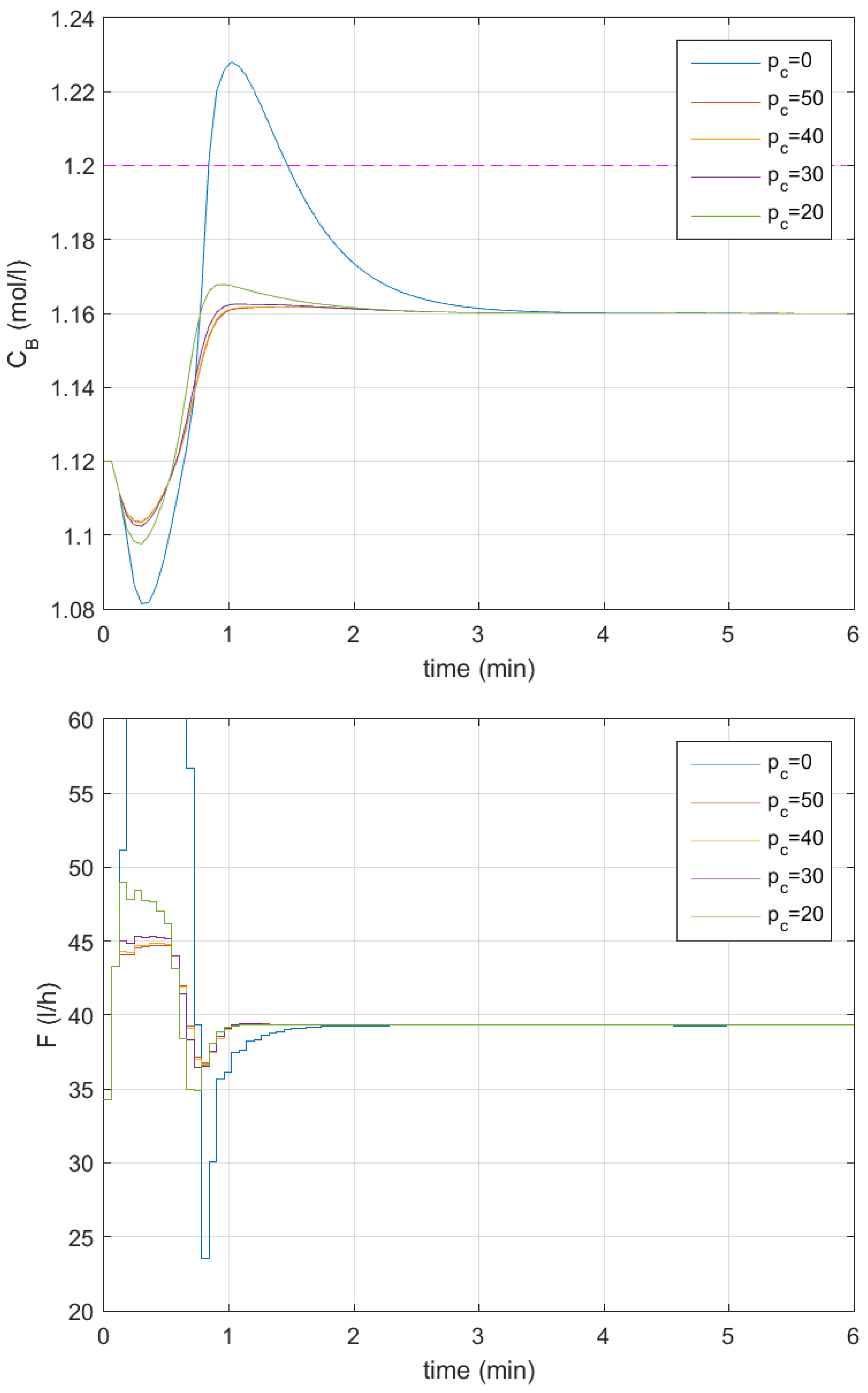
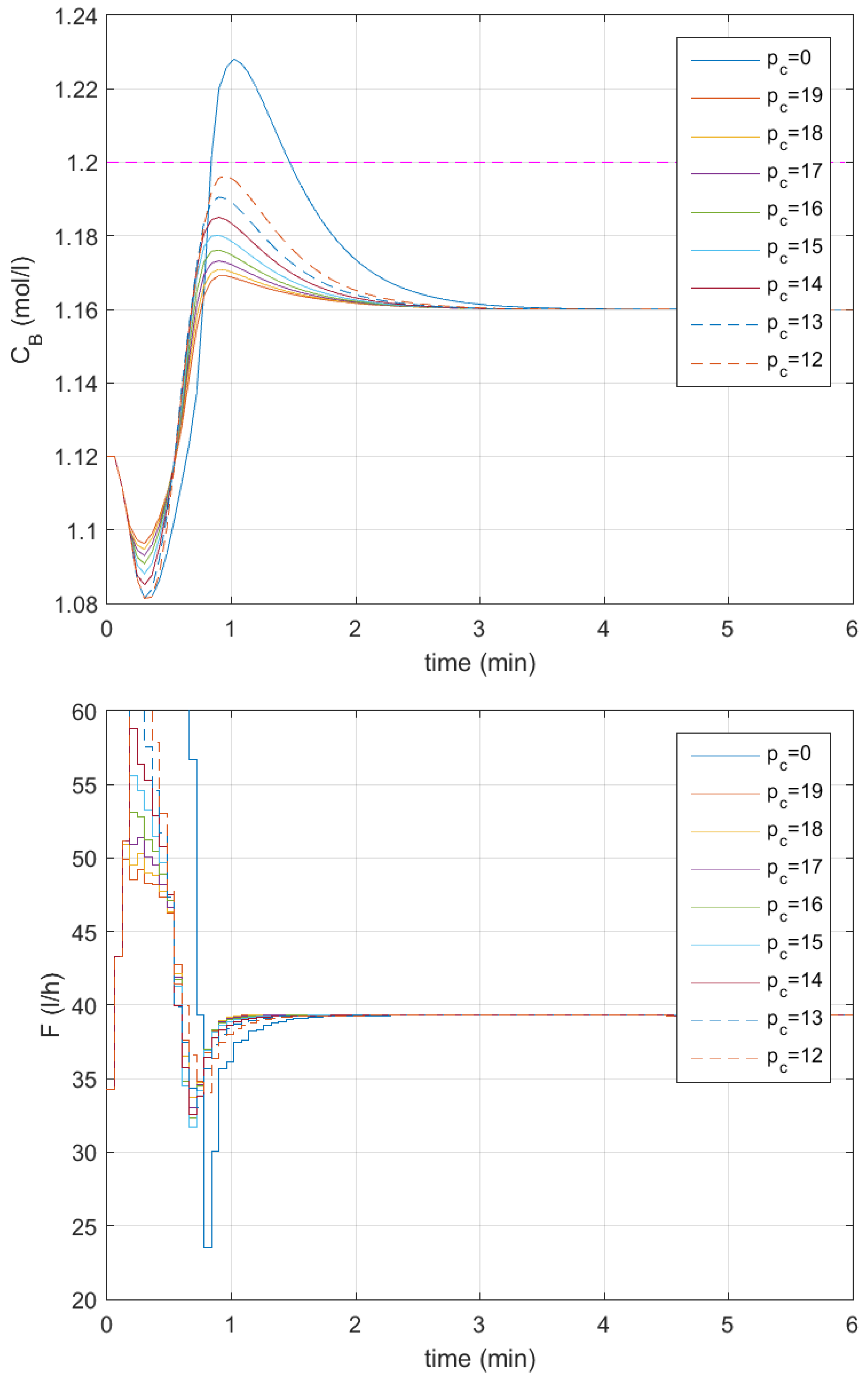
Next, the output constraint satisfaction mechanism with the output constraint located closer to setpoint C ¯ B 1 = 1.16 mol/L is tested, checking the same range of values of the constraint horizon as in the previous experiments (Figure 10 and Figure 11), with values of obtained control quality indicators placed in Table 5. This time, the upper output constraint is set on C B , m a x = 1.2 mol/L. The smallest values of the control quality indicators are obtained for constraint horizon p c [ 50 , 70 ] : the overshoot drops to 4.5 % , the settling time is reduced to t s = 0.9 min, the SSE is reduced 3 times, the SAE is reduced more than 2.5 times, the control effort indicator CE2 is reduced more than 8 times and the CE1 indicator is reduced more than 3.5 times. When the constraint horizon is decreased to p c = 30 , the control quality indicators grow gradually—the overshoot grows to 6.3 % and the settling time grows to t s = 1.56 min. When the constraint horizon is decreased to p c = 20 , the overshoot grows rapidly (to 19.6 % ), as do the SAE, CE2, and CE1 indicators. The SSE increases only slightly, and the settling time increases to t s = 1.86 min. However, the control quality indicators are still much smaller than in the case where the output constraint satisfaction mechanism is not employed.
In the following test, the constraint horizon is changed between p c = 19 and p c = 12 . All the control quality indicators gradually increase with an decrease in the constraint horizon, but the CE2 and CE1 indicators achieve their largest values for p c = 13 . Despite the mentioned growth of the control quality indicators, they are much smaller than in the reference case where the constraint satisfaction mechanism is not used—even for constraint horizon p c = 12 , the overshoot is equal to around 91 % , the settling time is t s = 2.34 min, the SSE is 1.7 times smaller, the SAE is 1.5 times smaller, the CE2 indicator is 2.5 times smaller and the CE1 indicator is more than 1.3 times smaller. Moreover, in all cases, the output signal does not violate the constraint.
The experiments illustrate the general properties of the proposed mechanism well. First, there is a set of values of the constraint horizon for which differences in the obtained responses are relatively small (between p c = 70 and p c = 40 ). However, as the mechanism is based on prediction, further decrease of the constraint horizon causes the response to deteriorate, because the prediction becomes too short. Therefore, it is advisable to first choose as long a constraint horizon as possible (as the resources allow) and then gradually decrease it until a deterioration in the control system operation occurs. Of course, it is also advisable to include modeling uncertainty in the prediction. The better the prediction, the more effective the proposed mechanism’s operation is. Summarizing, in the next experiments, the constraint horizon is assumed to be no smaller than p c = 20 .
Experiments were also conducted to test the robustness of the proposed mechanism. In Figure 12, responses of the control system to the change in the setpoint to C ¯ B 1 = 1.16 mol/L are obtained, where the output is subject to a measurement noise, which is simulated as random numbers from the interval [ 0.01 , 0.01 ] added to the output measurement sent to the controller with the proposed mechanism. Small oscillations are observed in the obtained responses, but the proposed mechanism operates without issues. Table 6 compares the control quality indicators obtained before and after adding measurement noise to the process output. In the case of all indicators except CE1, differences in their values depend more on the control horizon than on the noise added to the process output. The constraint is not violated, and the proposed mechanism works well.
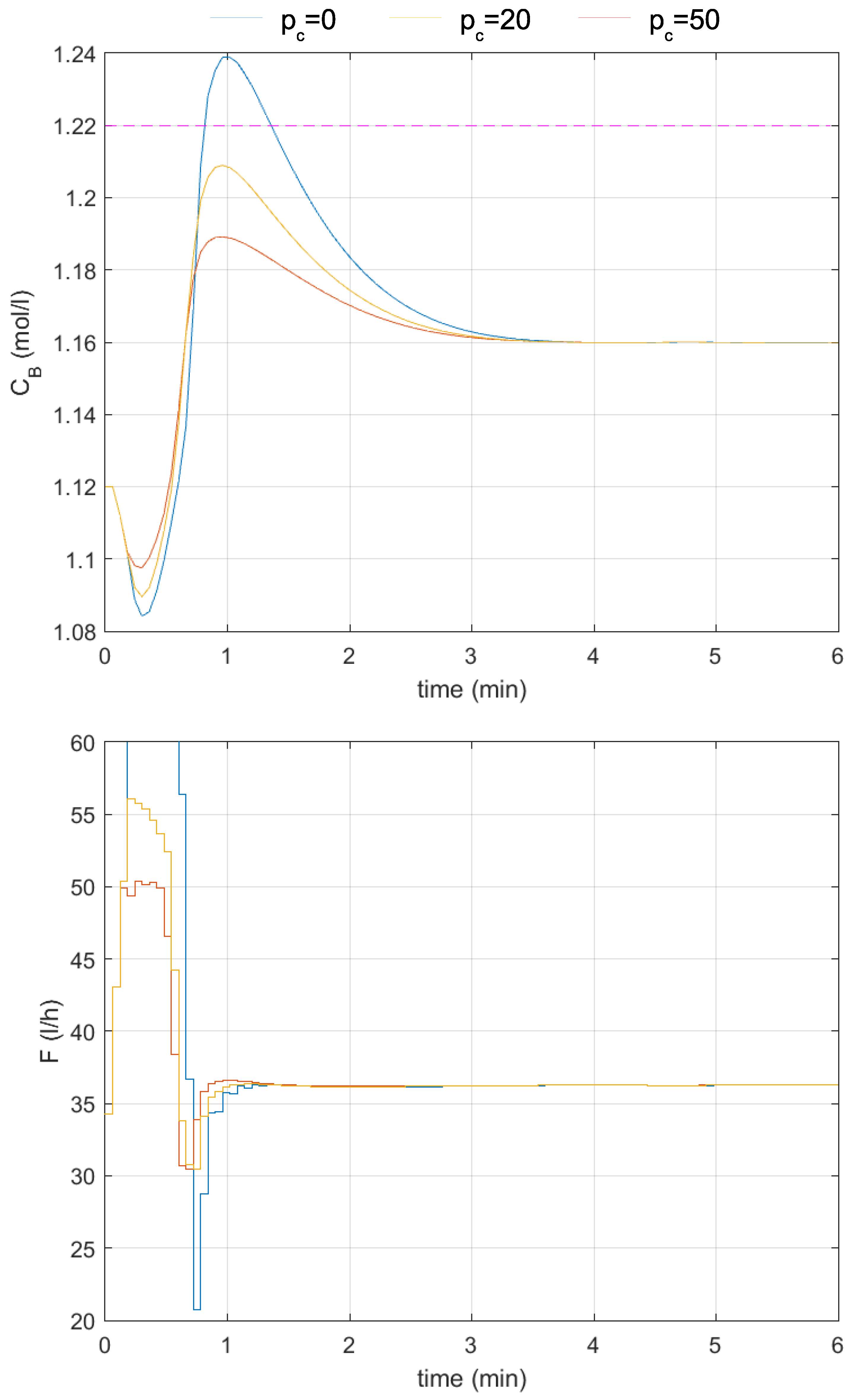
Experiments with a decrease in the value of the k 3 parameter by 10 % to k 3 = 9 L / ( h · mol ) were also conducted. The obtained responses of the control system to the change in the setpoint to C ¯ B 1 = 1.16 mol/L are shown in Figure 13, and the obtained values of the control quality indicators are placed in Table 7. The output constraint is violated in the reference case (no output constraint satisfaction mechanism, p c = 0 ), with responses worse than those obtained with the nominal value of the k 3 parameter (values of all control quality indicators increase compared to the similar case in Table 4). The mechanism of output constraint satisfaction works well. Two cases are tested, with control horizons p c = 50 and p c = 20 , and in both cases, the constraint is not violated. Moreover, the values of all control quality indicators improved compared to the reference case. In the case of overshoot, settling time, SSE, and SAE, the respective values are larger than in the nominal case (with the k 3 parameter unchanged compared to similar cases in Table 4). However, the control effort indicator CE2 remains almost unchanged for p c = 50 and decreases for p c = 20 . The CE1 indicator decreases in both cases ( p c = 50 and p c = 20 ).
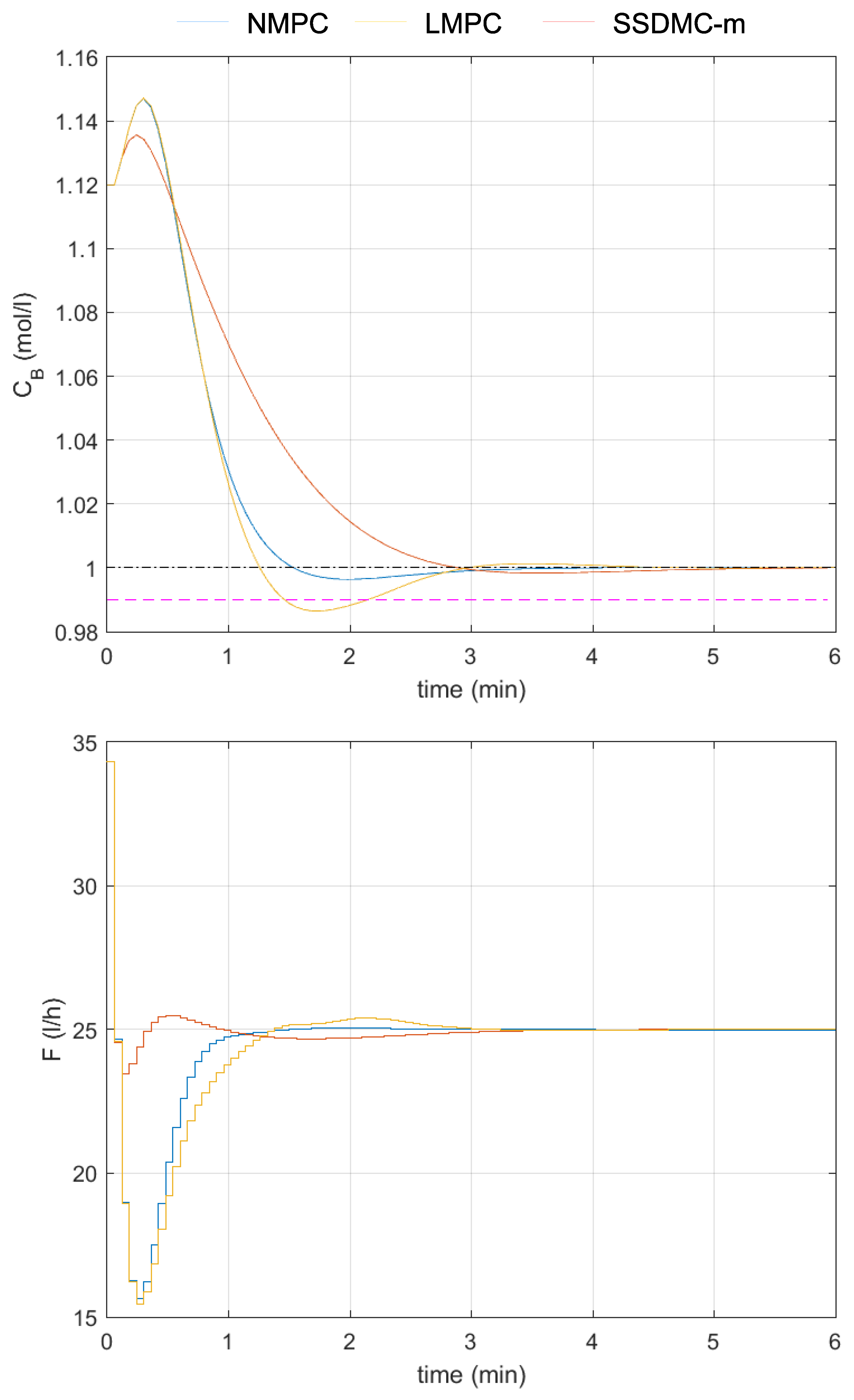
An attempt is also made to compare the effectiveness of the proposed approach to the standard ones (NMPC and LMPC). However, the overshoot generated in the control system with the NMPC algorithm, even after the detuning of the algorithm, was too small (less than 3–4%). Therefore, a reasonable comparison to make is one of the duration of each algorithm operation. Thus, the duration of action of standard optimization-based MPC algorithms that take output constraints into consideration (NMPC and LMPC) is compared to that of the SSDMC algorithm equipped with the proposed mechanism for satisfying output constraints. The parameters of all the controllers are assumed to be the same, namely, prediction horizon p = 70 and control horizon s = 35 , λ = 10 4 , and the constraint horizon in the SSDMC algorithm is assumed to be equal to p c = 70 . Thus, the output constraints in all cases are taken into account on the whole prediction horizon. However, in the case of NMPC and LMPC algorithms, two versions of implementation were tested: with only lower constraints (70 constraints) or with both lower and upper constraints (140 constraints). The lower output constraint was set to C B , m i n = 0.99 mol/L and the upper one to C B , m a x = 1.15 mol/L.
The responses of the tested control systems to the change in the setpoint to C ¯ B 1 = 1 mol/L are shown in Figure 14. The durations of action of each algorithm are compared in Table 8. For each algorithm, five measurements of duration are taken (the time needed to simulate the control plant is subtracted) and averaged. The NMPC algorithm is the slowest of the three, being more than 28 times slower than the LMPC algorithm, which utilizes standard quadratic programming to calculate the control action. If, in the NMPC algorithm, only lower constraints are taken into consideration, then it works 1.5 times faster. In the case of the LMPC algorithm, it works 1.4 times faster in the same case. The SSDMC algorithm, equipped with the tested mechanism, is the fastest one—more than 10 times faster than the LMPC algorithm with only lower constraints.
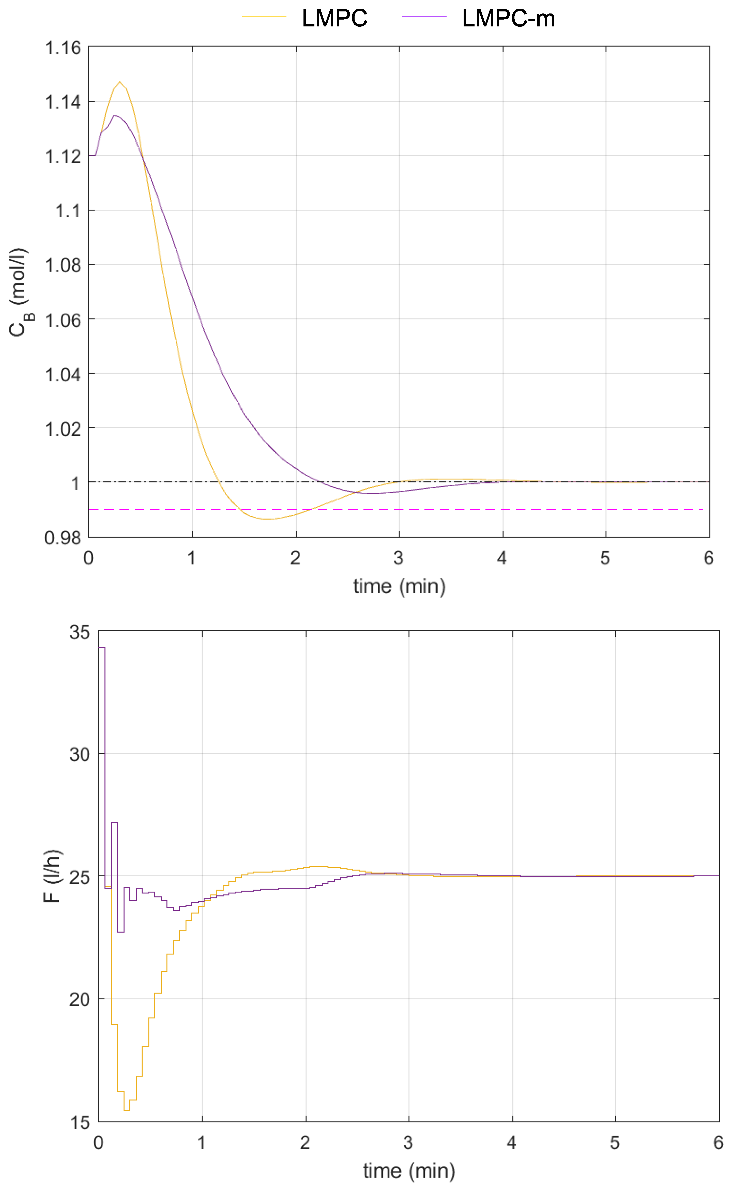
The responses generated with the LMPC algorithm violate the lower constraint, and the soft output constraints have to be implemented. This is caused by significant inaccuracy in the linear model that the algorithm is based on. However, the proposed mechanism for satisfying output constraints is based on formulas that linearly depend on decision variables (see constraints (8) and (9)) because it skillfully exploits the fuzzy model. Thus, these formulas have been used to define the output constraints in the optimization problem solved by the LMPC algorithm. The obtained response, as shown in Figure 15, is slow, but the constraint is not violated at this time. Using the fuzzy model improved the prediction and fulfilled the constraint. Moreover, the time required to obtain the control action is more than twice as short as in the LMPC algorithm, which takes into account all output constraints. Thus, the proposed mechanism can also be applied to existing implementations of the LMPC algorithms to improve their operation.

4. Discussion & Conclusions

The proposed mechanism for output constraint satisfaction is based on an easily obtainable fuzzy model composed of step responses and prediction generation, which is known from MPC algorithms. The mechanism utilizes the prediction to skillfully modify the control signal generated by the controller, ensuring that the output constraints are fulfilled. The mechanism is relatively easy to apply and can be used in any control system of a nonlinear process with a controller based on a control law. The effectiveness of the mechanism was successfully demonstrated in the control system of a nonminimum-phase, nonlinear control plant. We also detailed how to assess and incorporate information about modeling uncertainty into the proposed mechanism, demonstrating the importance of this issue in an example. The proposed mechanism is not only effective in preventing violations of the output constraints but also allows the user to improve the control quality offered by the control system in terms of settling time and overshoot, yielding a notable additional benefit.
The proposed mechanism, thanks to the possible incorporation of constraints (8) and (9) into the optimization problem, can also be used to relatively easily improve the operation of the standard MPC implementation based on quadratic optimization, like LMPC algorithms. This is because the mentioned constraints are linear with respect to one of the decision variables.
To sum up, the proposed mechanism can, in favorable circumstances, positively influence control quality, allowing us to
  • Obtain a higher quality of the product, thanks to the fulfillment of quality constraints;
  • Reduce losses when avoiding (or limiting the occurrence of) situations where the product does not meet the requirements in the event of exceeding the constraints;
  • Obtain economic benefits resulting from the above points.

Author Contributions

Conceptualization, P.M.; methodology, P.M.; software, P.M.; validation, P.M.; formal analysis, P.M.; investigation, P.M.; resources, P.M.; data curation, P.M.; writing—original draft preparation, P.M.; writing—review and editing, E.N.-S. and P.M.; visualization, P.M.; supervision, E.N.-S. All authors have read and agreed to the published version of the manuscript.

Funding

This research received no external funding.

Institutional Review Board Statement

Not applicable.

Informed Consent Statement

Not applicable.

Data Availability Statement

The original contributions presented in this study are included in the article. Further inquiries can be directed to the corresponding author.

Conflicts of Interest

The authors declare no conflicts of interest.

Abbreviations

The following abbreviations are used in this manuscript:
CE1Control Effort Indicator 1
CE2Control Effort Indicator 2
LMPCMPC Based on Linear Lodel
MPCModel Predictive Control
NMPCNonlinear MPC
PIDProportional–Integral–Derivative
SAESum of Absolute Errors
SSESum of Squared Errors

References

  1. Yuan, M.; Manzie, C.; Good, M.; Shames, I.; Gan, L.; Keynejad, F.; Robinette, T. A Review of Industrial Tracking Control Algorithms. Control Eng. Pract. 2020, 102, 104536. [Google Scholar]
  2. Yuan, M.; Manzie, C.; Good, M.; Shames, I.; Gan, L.; Keynejad, F.; Robinette, T. Error–Bounded Reference Tracking MPC for Machines With Structural Flexibility. IEEE Trans. Ind. Electron. 2020, 67, 8143–8154. [Google Scholar]
  3. Garone, E.; Di Cairano, S.; Kolmanovsky, I. Reference and Command Governors for Systems with Constraints: A Survey on Theory and Applications. Automatica 2017, 75, 306–328. [Google Scholar] [CrossRef]
  4. Nebeluk, R.; Ławryńczuk, M. Tuning of Nonlinear MPC Algorithm for Vehicle Obstacle Avoidance. In Advanced, Contemporary Control. Advances in Intelligent Systems and Computing; Bartoszewicz, A., Kabziński, J., Kacprzyk, J., Eds.; Springer: Cham, Switzerland, 2020; Volume 1196, pp. 595–615. [Google Scholar]
  5. Perera, Y.S.; Li, J.; Abeykoon, C. Melt Viscosity Control in Polymer Extrusion Using Nonlinear Model Predictive Control with Neural State Space Modelling and Soft Sensor Feedback. J. Process Control 2025, 155, 103556. [Google Scholar]
  6. Tatjewski, P. Offset–Free Nonlinear Model Predictive Control with State–Space Process Models. Arch. Control Sci. 2017, 27, 595–615. [Google Scholar] [CrossRef]
  7. Schäfer, A.; Kühl, P.; Diehl, M.; Schlöder, J.; Bock, H.G. Fast Reduced Multiple Shooting Methods for Nonlinear Model Predictive Control. Chem. Eng. Process. 2007, 46, 1200–1214. [Google Scholar] [CrossRef]
  8. Zavala, V.M.; Laird, C.D.; Biegler, L.T. A Fast Moving Horizon Estimation Algorithm Based on Nonlinear Programming Sensitivity. J. Process Control 2008, 18, 876–884. [Google Scholar]
  9. Ławryńczuk, M.; Nebeluk, R. Beyond the Quadratic Norm: Computationally Efficient Constrained Nonlinear MPC Using a Custom Cost Function. ISA Trans. 2023, 134, 336–356. [Google Scholar]
  10. Marusak, P.M. Designing Efficient Model Predictive Control Algorithm Using Easy–to–Obtain Fuzzy Models. Int. J. Electron. Telecommun. 2025, 71, 1–8. [Google Scholar]
  11. Nebeluk, R.; Ławryńczuk, M. Computationally Simple Nonlinear MPC Algorithm for Vehicle Obstacle Avoidance With Minimization of Fuel Utilization. IEEE Access 2021, 9, 17296–17311. [Google Scholar] [CrossRef]
  12. Dominguez, L.F.; Pistikopoulos, E.N. A Novel mp-NLP Algorithm for Explicit/Multi-parametric NMPC. In Proceedings of the 8th IFAC Symposium on Nonlinear Control Systems, Bologna, Italy, 1–3 September 2010. [Google Scholar]
  13. Johansen, T.A. On multi–parametric nonlinear programming and explicit nonlinear model predictive control. In Proceedings of the 41st IEEE Conference on Decision and Control, Las Vegas, NV, USA, 10–13 December 2002; Volume 3, pp. 2768–2773. [Google Scholar]
  14. Johansen, T.A. Approximate explicit receding horizon control of constrained nonlinear systems. Automatica 2004, 40, 293–300. [Google Scholar] [CrossRef]
  15. Bemporad, A.; Borrelli, F.; Morari, M. Piecewise linear optimal controllers for hybrid systems. In Proceedings of the 2000 American Control Conference, Chicago, IL, USA, 28–30 June 2000; Volume 2, pp. 1190–1194. [Google Scholar]
  16. Bemporad, A.; Morari, M.; Dua, V.; Pistikopoulos, E.N. The explicit linear quadratic regulator for constrained systems. Automatica 2002, 38, 3–20. [Google Scholar] [CrossRef]
  17. Pistikopoulos, E.N.; Dua, V.; Bozinis, N.A.; Bemporad, A.; Morari, M. On–line optimization via off–line parametric optimization tools. Comput. Chem. Eng. 2002, 26, 175–185. [Google Scholar] [CrossRef]
  18. Chaber, P.; Ławryńczuk, M. Fast Analytical Model Predictive Controllers and Their Implementation for STM32 ARMmicrocontroller. IEEE Trans. Ind. Inform. 2019, 15, 4580–4590. [Google Scholar] [CrossRef]
  19. Wojtulewicz, A.; Ławryńczuk, M. Computationally Efficient Implementation of Dynamic Matrix Control Algorithm for Very Fast Processes Using Programmable Logic Controller. In Proceedings of the 23rd International Conference on Methods and Models in Automation and Robotics (MMAR), Międzyzdroje, Poland, 27–30 August 2018; pp. 579–584. [Google Scholar]
  20. Marusak, P.M.; Kuntanapreeda, S. Output Constrained IMC Controllers In Control Systems of Electromechanical Actuators. Control Theory Technol. 2015, 13, 245–255. [Google Scholar] [CrossRef]
  21. Piegat, A. Fuzzy Modeling and Control; Physica–Verlag: Heidelberg, Germany, 2001. [Google Scholar]
  22. Takagi, T.; Sugeno, M. Fuzzy Identification of Systems and Its Application to Modeling and Control. IEEE Trans. Syst. Man Cybern. 1985, 15, 116–132. [Google Scholar] [CrossRef]
  23. Li, J.; Lewis, H.W. Fuzzy Clustering Algorithms—Review of the Applications. In Proceedings of the 2016 IEEE International Conference on Smart Cloud (SmartCloud), New York, NY, USA, 18–20 November 2016; pp. 282–288. [Google Scholar]
  24. Tatjewski, P. Advanced Control of Industrial Processes: Structures and Algorithms; Springer: London, UK, 2007. [Google Scholar]
  25. Marusak, P.M. Analytical MPC Algorithm Using Steady-State Process Model. Algorithms 2025, 18, 79. [Google Scholar] [CrossRef]
  26. Okienková, K.; Dodek, M.; Málik, R.; Paulusová, J.; Tárník, M. Robust Model Predictive Control of the Van De Vusse Reaction with Uncertain Extended Prediction Model and LMI–Based Design. IEEE Access 2025, 13, 182088–182106. [Google Scholar] [CrossRef]
  27. Krishna, D.; Suryanarayana, K.; Aparna, G.; Padma Sree, R. Tuning of PID controllers for continuous stirred tank reactors. Indian Chemical Engineer 2012, 54, 157–179. [Google Scholar] [CrossRef]
  28. Marusak, P.M. A numerically efficient fuzzy MPC algorithm with fast generation of the control signal. Int. J. Appl. Math. Comput. Sci. 2021, 31, 59–71. [Google Scholar] [CrossRef]
  29. Doyle, F.; Ogunnaike, B.A.; Pearson, R.K. Nonlinear Model–Based Control Using Second–Order Volterra Models. Automatica 1995, 31, 697–714. [Google Scholar] [CrossRef]
Figure 1. The structure of the control system.
Applsci 16 00928 g001
Figure 2. Normalized step responses (parameters of local models); local model for small C B (parameters a n 1 )—blue line, local model for medium C B (parameters a n 2 )—red line, local model for large C B (parameters a n 3 )—yellow line.
Applsci 16 00928 g002
Figure 3. A comparison of the process model output with the output of the linear model obtained for medium values of output C B ; the output of the original model—blue lines, the output of the linear model—dashed red lines; top—output trajectories, bottom—input trajectory.
Applsci 16 00928 g003
Figure 4. A comparison of the process model output with the output of the fuzzy model composed of two step responses (top); the output of the original model—blue lines, the output of the fuzzy model—dashed red lines; bottom—membership functions of the fuzzy model (their colors correspond to the colors of step responses in Figure 2).
Applsci 16 00928 g004
Figure 5. A comparison of the process model output with the output of the fuzzy model composed of three step responses (top); the output of the original model—blue lines, the output of the fuzzy model—dashed red lines; bottom—membership functions of the fuzzy model (their colors correspond to the colors of step responses in Figure 2).
Applsci 16 00928 g005
Figure 6. Responses of the control system to the change in the setpoint of the control system to the change in the setpoint to C ¯ B 1 = 1.16 mol/L; no output constraint satisfaction mechanism—blue lines, p c = 50 —red lines, p c = 40 —yellow lines, p c = 30 —lilac lines, p c = 20 —green lines; upper output constraint C B , m a x = 1.22 mol/L—the dashed magenta line; without the inclusion of modeling uncertainty.
Applsci 16 00928 g006
Figure 7. Responses of the control system to the change in the setpoint of the control system to the change in the setpoint to C ¯ B 1 = 1.16 mol/L; no output constraint satisfaction mechanism—blue lines, p c = 19 —red lines, p c = 18 —yellow lines, p c = 17 —lilac lines, p c = 16 —green lines, p c = 15 —cyan lines, p c = 14 —brown lines, p c = 13 —dashed blue lines, p c = 12 —dashed red lines; upper output constraint C B , m a x = 1.22 mol/L—the dashed magenta line; without the inclusion of modeling uncertainty.
Applsci 16 00928 g007
Figure 8. Responses of the control system to the change in the setpoint to C ¯ B 1 = 1.16 mol/L; no output constraint satisfaction mechanism—blue lines, p c = 50 —red lines, p c = 40 —yellow lines, p c = 30 —lilac lines, p c = 20 —green lines; upper output constraint C B , m a x = 1.22 mol/L—the dashed magenta line; the modeling inaccuracy assessment employed.
Applsci 16 00928 g008
Figure 9. Responses of the control system to the change in the setpoint to C ¯ B 1 = 1.16 mol/L; no output constraint satisfaction mechanism—blue lines, p c = 19 —red lines, p c = 18 —yellow lines, p c = 17 —lilac lines, p c = 16 —green lines, p c = 15 —cyan lines, p c = 14 —brown lines, p c = 13 —dashed blue lines, p c = 12 —dashed red lines; upper output constraint C B , m a x = 1.22 mol/L—the dashed magenta line; the modeling inaccuracy assessment employed.
Applsci 16 00928 g009
Figure 10. Responses of the control system to the change in the setpoint to C ¯ B 1 = 1.16 mol/L; no output constraint satisfaction mechanism—blue lines, p c = 50 —red lines, p c = 40 —yellow lines, p c = 30 —lilac lines, p c = 20 —green lines; upper output constraint C B , m a x = 1.2 mol/L—the dashed magenta line; the modeling inaccuracy assessment employed.
Applsci 16 00928 g010
Figure 11. Responses of the control system to the change in the setpoint to C ¯ B 1 = 1.16 mol/L; no output constraint satisfaction mechanism—blue lines, p c = 19 —red lines, p c = 18 —yellow lines, p c = 17 —lilac lines, p c = 16 —green lines, p c = 15 —cyan lines, p c = 14 —brown lines, p c = 13 —dashed blue lines, p c = 12 —dashed red lines; upper output constraint C B , m a x = 1.2 mol/L—the dashed magenta line; the modeling inaccuracy assessment employed.
Applsci 16 00928 g011
Figure 12. Responses of the control system to the change in the setpoint to C ¯ B 1 = 1.16 mol/L; p c = 50 —blue lines, p c = 20 —red lines; upper output constraint C B , m a x = 1.22 mol/L—the dashed magenta line; measurement noise is added.
Applsci 16 00928 g012
Figure 13. Responses of the control system to the change in the setpoint to C ¯ B 1 = 1.16 mol/L; no output constraint satisfaction mechanism—blue lines, p c = 50 —red lines, p c = 20 —yellow lines; upper output constraint C B , m a x = 1.22 mol/L—the dashed magenta line; parameter k 3 in the process model changed by 10 % to k 3 = 9 l / ( h · mol ) .
Applsci 16 00928 g013
Figure 14. Responses of the control systems with different control algorithms to the change in the setpoint to C ¯ B 1 = 1 mol/L (dash–dotted black line); NMPC—blue lines, SSDMC with the proposed mechanism—red lines, LMPC—yellow lines; lower output constraint C B , m a x = 0.99 mol/L—the dashed magenta line.
Applsci 16 00928 g014
Figure 15. Responses of the control system with the LMPC algorithm to the change in the setpoint to C ¯ B 1 = 1 mol/L (dash–dotted black line); classical LMPC—yellow lines, LMPC with the proposed mechanism—lilac lines; lower output constraint C B , m a x = 0.99 mol/L—the dashed magenta line.
Applsci 16 00928 g015
Table 1. SSEs of simplified process models.
One Local Model (Figure 3)Two Local Models (Figure 4)Three Local Models (Figure 5)
9.30972.00130.3568
Table 2. Values of y 0 f and u 0 f parameters in the fuzzy model.
ParameterLocal Model #1
(f = 1)
Local Model #2
(f = 2)
Local Model #3
(f = 3)
y 0 f 0.911.121.22
u 0 f 20.1034.3049.98
Table 3. Control quality indicators of responses from Figure 6 and Figure 7.
p c ResponseOvershoot (%) t s (min)SSESAECE2CE1
0Figure 6 blue lines170.242.820.08691.6704860.338678.0063
50–70Figure 6 red lines48.272.100.03490.8442242.685540.8727
40Figure 6 yellow lines49.412.100.03510.8500249.213341.5072
30Figure 6 lilac lines54.702.160.03640.8772277.911043.9890
20Figure 6 green lines82.112.340.04491.0468320.783851.1836
19Figure 7 red lines88.332.340.04731.0907342.058652.8462
18Figure 7 yellow lines94.882.400.05031.1424370.069553.5927
17Figure 7 lilac lines102.592.460.05411.2100375.855251.4157
16Figure 7 green lines109.332.580.05951.3130371.547150.8686
15Figure 7 cyan lines118.142.760.06811.4768347.704750.3047
14Figure 7 brown lines124.612.940.07641.6269339.539451.1416
13Figure 7 dashed blue lines133.773.360.09702.0008307.744450.4045
12Figure 7 dashed red lines143.874.200.14512.8255331.107150.8947
Table 4. Control quality indicators of responses from Figure 8 and Figure 9.
p c ResponseOvershoot (%) t s (min)SSESAECE2CE1
0Figure 8 blue lines170.242.820.08691.6704860.338678.0063
50–70Figure 8 red lines61.102.220.03780.9244278.287646.2883
40Figure 8 yellow lines62.652.220.03830.9332286.310746.9795
30Figure 8 lilac lines69.922.220.04030.9754324.018450.1329
20Figure 8 green lines104.432.460.05311.1946437.921759.1939
19Figure 9 red lines111.952.460.05661.2472467.868160.6568
18Figure 9 yellow lines121.552.520.06121.3155482.700261.7352
17Figure 9 lilac lines131.292.580.06651.3898479.935963.1520
16Figure 9 green lines140.912.640.07151.4623487.903060.1499
15Figure 9 cyan lines152.242.760.07801.5646441.779957.1858
14Figure 9 brown lines155.222.820.08271.6402421.054256.0484
13Figure 9 dashed blue lines155.032.940.09141.7868432.691057.4629
12Figure 9 dashed red lines155.143.060.09771.8908469.675857.6537
Table 5. Control quality indicators of responses from Figure 10 and Figure 11.
p c ResponseOvershoot (%) t s (min)SSESAECE2CE1
0Figure 10 blue lines170.242.820.08691.6704860.338678.0063
50–70Figure 10 red lines4.460.900.02800.6448100.249221.2585
40Figure 10 yellow lines4.670.840.02800.6451101.491921.6521
30Figure 10 lilac lines6.281.560.02820.6473107.958523.5195
20Figure 10 green lines19.601.860.02980.6851166.685934.6227
19Figure 11 red lines22.761.860.03030.6982185.907937.5764
18Figure 11 yellow lines27.131.920.03100.7141211.876141.0680
17Figure 11 lilac lines32.961.920.03220.7417227.978742.2610
16Figure 11 green lines40.311.980.03380.7824251.752846.6740
15Figure 11 cyan lines50.362.100.03630.8394285.259952.8949
14Figure 11 brown lines62.562.160.03970.9105324.909557.5839
13Figure 11 dashed blue lines76.352.280.04420.9966346.769159.0407
12Figure 11 dashed red lines90.712.340.04921.0972341.148956.9986
Table 6. Control quality indicators of responses from Figure 8 (no noise) and Figure 12 (with noise).
p c ResponseOvershoot (%) t s (min)SSESAECE2CE1
50Figure 8 red lines no noise61.102.220.03780.9244278.287646.2883
50Figure 12 blue lines with noise57.352.100.03730.9289270.759461.4439
20Figure 8 green lines no noise104.432.460.05311.1946437.921759.1939
20Figure 12 red lines with noise104.542.520.05291.2180441.431774.8157
Table 7. Control quality indicators of responses from Figure 13.
p c ResponseOvershoot (%) t s (min)SSESAECE2CE1
0Figure 13 blue lines197.373.120.10971.9886975.732781.4058
50Figure 13 red lines72.962.820.03821.0789278.098143.8559
20Figure 13 yellow lines122.482.880.05991.4180366.719253.6553
Table 8. The average duration of action of the algorithms (s) in the experiments from Figure 14 and Figure 15.
NMPC–ulNMPC–lLMPC–ulLMPC–lLMPC–mSSDMC–m
158.5268105.94655.49053.84862.51300.3305
ul—upper and lower output constraints taken into consideration, l—only lower output constraints taken into consideration, m—the proposed mechanism with upper and lower output constraints.
Disclaimer/Publisher’s Note: The statements, opinions and data contained in all publications are solely those of the individual author(s) and contributor(s) and not of MDPI and/or the editor(s). MDPI and/or the editor(s) disclaim responsibility for any injury to people or property resulting from any ideas, methods, instructions or products referred to in the content.