Research on Defect Detection on Steel Rails Based on Improved YOLO11n Algorithm

Abstract

Aiming at the core issues of the traditional YOLO11n model in rail surface defect detection—fine-grained feature loss of small defects, insufficient micro-target recognition accuracy, and the mismatch of existing downsampling/fusion methods for micro-defect feature extraction—this paper proposes an improved YOLO11n algorithm with two-dimensional network structure innovations. First, the Adaptive Downsampling (ADown) module is introduced into the backbone network for the first time, retaining global features via 2D average pooling and extracting local details through channel-split multi-path convolution/max pooling to avoid fine texture loss. Second, the original SOEP-RFPN-MFM neck network is designed, integrating SNI, GSConvE and MFM modules to achieve dynamic weighted fusion of multi-scale features and break the bottleneck of inefficient small-target feature aggregation. Trained and verified on a 4020-image rail dataset covering four defect types (Spalling, Squat, Wheel Burns, Corrugation), the improved algorithm achieves 93.7% detection accuracy, 92.4% recall and 95.6% mAP, realizing incremental improvements of 1.2, 2.6 and 0.8 percentage points, respectively, compared with the original YOLO11n, which is particularly optimized for rail micro-defect detection scenarios. This study provides a new deep learning method for rail transit micro-defect detection and a reference for scenario-specific improvement of lightweight YOLO11n models.

1. Introduction

As a vital national infrastructure, the safety and stability of railway tracks directly impact the lives of millions of passengers and the efficient operation of national logistics transportation [1]. With the rapid expansion of high-speed rail networks and increasing train speeds, tracks are highly susceptible to defects such as spalling [2], squat [3], wheel burn [4], and corrugation [5]. Failure to detect and repair these defects promptly may trigger major safety incidents (e.g., track deformation or train derailment) [6], making track defect detection an indispensable core component of railway operation and maintenance systems. Traditional railway defect detection mainly relies on manual inspections, where inspectors visually check or use handheld tools to identify defects in key areas such as rail surfaces and joints [7,8,9]. This method has obvious limitations: first, it is highly inefficient—given the complexity and extensiveness of current railway networks, comprehensive and frequent inspections are difficult to achieve with human resources alone, especially in complex scenarios like tunnels and bridges; and second, it is prone to the influence of inspectors’ subjective experience and fatigue, resulting in high rates of missed detection and false positives. Additionally, accurate identification of minute defects (e.g., microcracks smaller than 0.2 mm) is challenging. Furthermore, extreme weather conditions (e.g., heavy rainfall, high temperatures, and severe cold) further increase the risks and difficulties of manual inspections. This approach is clearly incompatible with modern railway operations’ requirements for “high density, high speed, and high safety.”

To overcome the limitations of traditional inspection methods, intelligent detection technologies have emerged. Among these, deep learning-based object detection algorithms—leveraging their powerful feature extraction and pattern recognition capabilities—have become the primary technical approach for automated defect detection in rail tracks. Among numerous object detection models, the YOLO (You Only Look Once) series is widely adopted in industrial quality inspection, intelligent surveillance, and other scenarios demanding strict real-time performance due to its “single-stage detection” capability. It achieves real-time inference while ensuring high detection accuracy [10]. As a lightweight iteration of the YOLO11 series, YOLO11n leverages a streamlined network architecture and optimized computational modules to achieve strong deployment capabilities on embedded edge devices. It strikes a balance between detection speed and model size, theoretically suitable for various mobile terminals such as track inspection robots.

However, directly applying YOLO11n to detect railway defects still reveals several adaptation challenges [11]. First, the original model’s standard convolution downsampling with fixed strides boosts computational efficiency but loses fine texture/edge information, hindering identification of early defects (e.g., microcracks, initial bolt loosening) amid normal wear. Second, the neck network’s feature fusion inadequately targets small defects; traditional upsampling/stitching fails to aggregate cross-scale features, reducing detection accuracy for small defects (e.g., rail oil stains) in complex scenes. Third, the model’s fixed receptive field cannot adapt to diverse rail defects (e.g., oblique cracks), compromising detection reliability.

It can be seen from the studies of Xin, Haitao and Song, Junpeng [12] in “YOLOv5-ACCOF Steel Surface Defect Detection Algorithm”, Chao, Chang et al. [13] in “IAMF-YOLO: Metal Surface Defect Detection Based on Improved YOLOv8”, and Dang, Zichen et al. [14] in “FD-YOLO11: A Feature-Enhanced Deep Learning Model for Steel Surface Defect Detection” that these three studies all fall into the field of “YOLO series + metal surface defect detection”, with their core objective being to improve detection accuracy and speed. They can be integrated from three dimensions: module fusion, unification of experimental benchmarks, and subdivision of application scenarios. However, the issues of “combinatorial innovation” in module improvement and the insufficient capability for few-shot and rare defect detection remain unaddressed.

To address the key research gaps—fixed-stride downsampling-induced fine defect detail loss, inadequate small defect feature fusion in the neck network, and fixed receptive fields’ inability to adapt to diverse rail defects—this paper proposes two core improvements based on YOLO11n: First, an adaptive downsampling module (ADown) replaces the original backbone [15]’s standard convolution downsampling; this module reduces feature map size via multi-path processing while preserving fine defect details, overcoming downsampling-related feature loss. Second, the SOEP-RFPN-MFM neck module is designed, integrating SNI [16], GSConvE [17], and MFM [18] to enhance fusion efficiency and minute feature representation, addressing the inadequacy of traditional neck networks in small defect feature fusion. These improvements aim to boost typical rail defect (e.g., spalling, indentation) detection accuracy and model reliability, providing efficient technical support for intelligent rail inspection and advancing the “automation, intelligence, and precision” transformation of railway operation and maintenance.

Research Objectives and Content

Based on the aforementioned background and issues, the core research objectives of this paper are as follows: First, to address the problem that the standard convolutional downsampling of the original YOLO11n loses rail micro-defect information, the Adaptive Downsampling (ADown) module is introduced to replace the backbone network structure, so as to retain fine defect features through multi-path extraction; Second, aiming at the limitation of inefficient small-target fusion in the neck network, the SOEP-RFPN-MFM neck network is originally designed; through multi-module collaboration, it optimizes multi-scale feature fusion and dynamic modulation to enhance the small-target representation capability; Third, the model is trained on the 4020-image rail dataset containing four defect types; the effectiveness of the modules is verified via ablation experiments, and the performance advantages of the model are quantified through comparative experiments; Fourth, a lightweight and high-precision solution is provided for intelligent rail detection, so as to promote the transformation of railway operation and maintenance toward “automation, intelligence, and precision”.

2. Network Architecture of YOLO11n

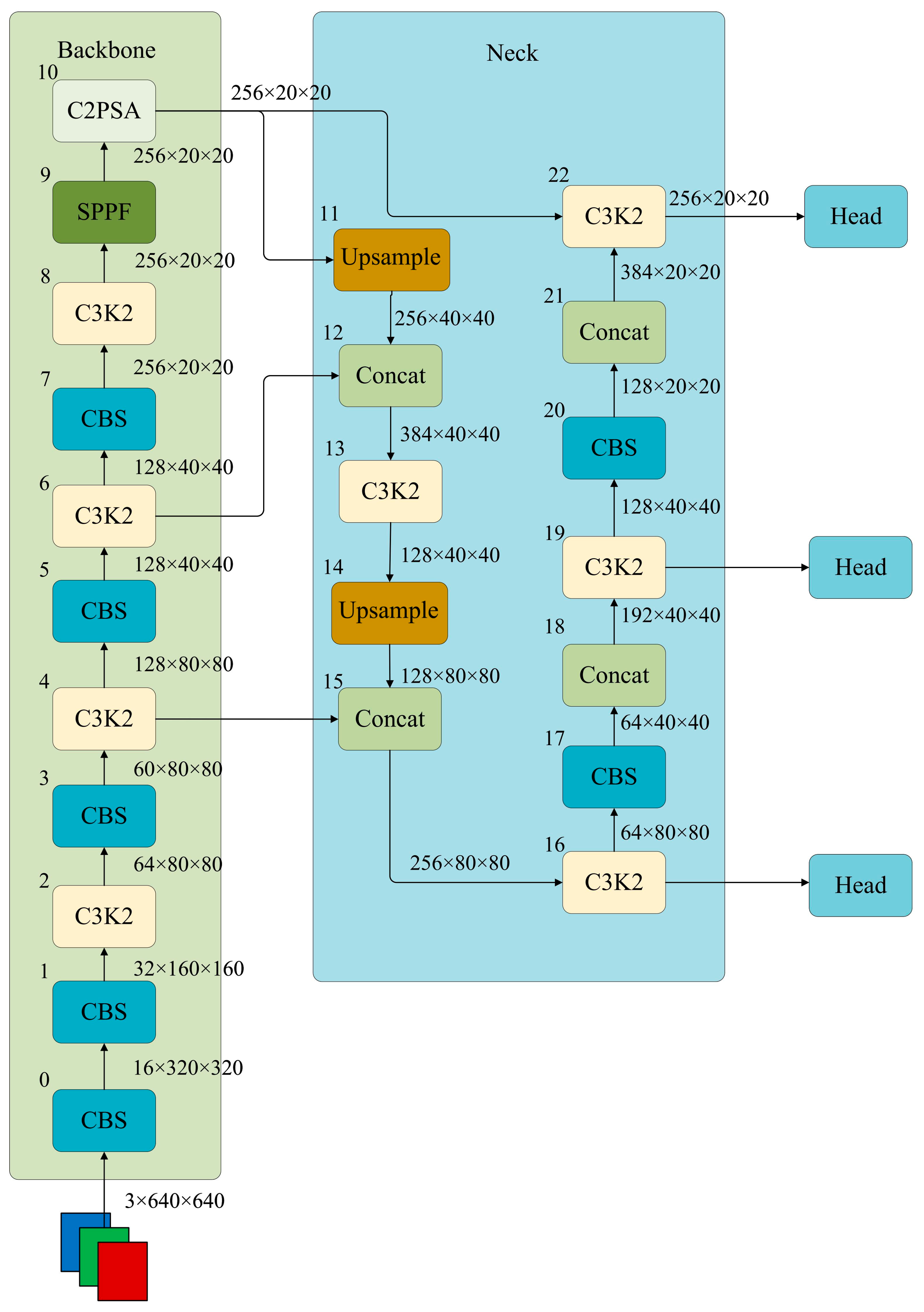
YOLO11, released by the Ultralytics team on September 30, 2024, is the latest addition to the YOLO (You Only Look Once) series. Compared to previous YOLO versions, it incorporates new features and enhancements while further improving performance and flexibility. This makes YOLO11 an ideal choice for various computer vision tasks including object detection and tracking, segmentation, image classification, and pose estimation [19]. YOLO11n, a lightweight variant of the YOLO11 series, adopts a three-part architecture: backbone network, neck network, and detection head [20]. This design balances detection speed with accuracy, as illustrated in Figure 1.

2.1. Backbone Network (Backbone)

The backbone network extracts multi-scale features from input images [21], comprising a convolutional block (CBS), cross-stage feature enhancement module (C3k2), spatial pyramid pooling (SPPF), and cross-stage partial pyramid slice attention (C2PSA).

The Convolution Block (CBS) consists of a 3 × 3 basic convolution module (Conv), Batch Normalization (BN), and the activation function (SiLU). It first applies a 2D convolutional layer, followed by a 2D batch—normalization layer whose formula is (1)–(4), activation function is used to gradually reduce the size of the feature map [22].

$${\mu }_c={\displaystyle \frac{1}{B·H·W}}\sum _{b=1}^B\sum _{h=1}^H\sum _{w=1}^W{x}_{b,c,h,w}$$

(1)

$${\sigma }_c^2={\displaystyle \frac{1}{B·H·W}}{\sum }_{b=1}^B{\sum }_{h=1}^H{\sum }_{w=1}^W{\left(x_{b,c,h,w}-{\mu }_c\right)}^2$$

(2)

$${\widehat{x}}_{b,c,h,w}={\displaystyle \frac{x_{b,c,h,w}-{\mu }_c}{\sqrt{{\sigma }_c^2-ϵ}}}$$

(3)

$$y_{b,c,h,w}={\gamma }_c·{\widehat{x}}_{b,c,h,w}+{\beta }_c$$

(4)

Among them, the input data is x ∈ R^B×C×H×W, where B represents the batch size, C represents the number of channels, H represents the height, and W represents the width. ${\widehat{x}}_i$ is the normalized value, $x_i$ is the input value ${\mu }_c$ is the mean value of $x$, ${\sigma }_c^2$ is the variance of $x$, and $\mathsf{ϵ}$ is a very small constant used to prevent division by zero operations.

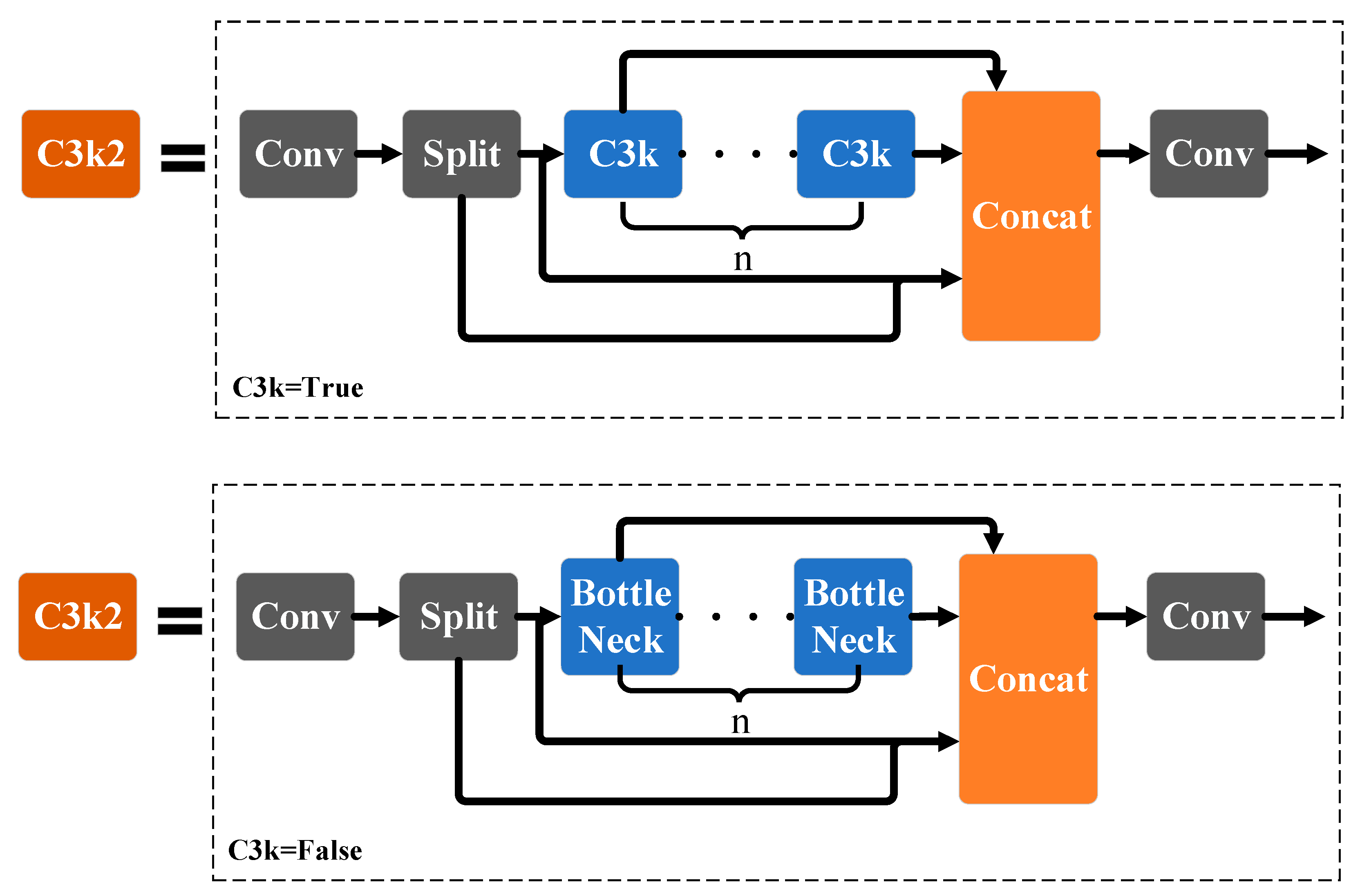
As shown in Figure 2, The cross-stage feature enhancement module (C3k2), a crucial component of the YOLO11 backbone network, evolved from the C2F module. When the C3k parameter is set to False or True, the Bottleneck in the C3k2 module is correspondingly replaced with a standard Bottleneck or C3 module. This allows the C3k in C3k2 to customize the convolution block size compared to C3. Furthermore, cross-layer connections fuse feature maps from different depths, enhancing the network’s ability to represent complex features. Simultaneously, the introduction of residual structures mitigates the vanishing gradient problem.

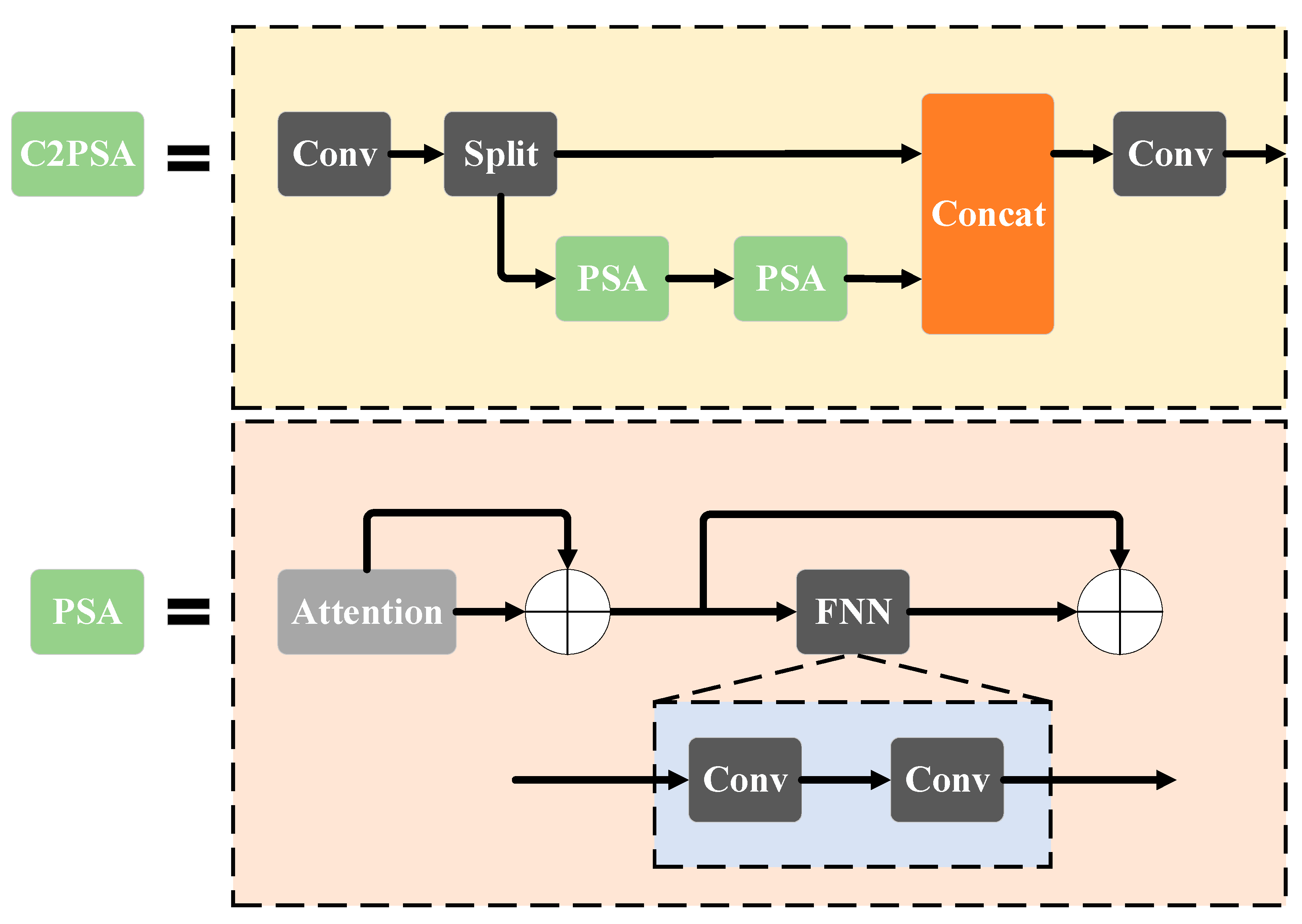
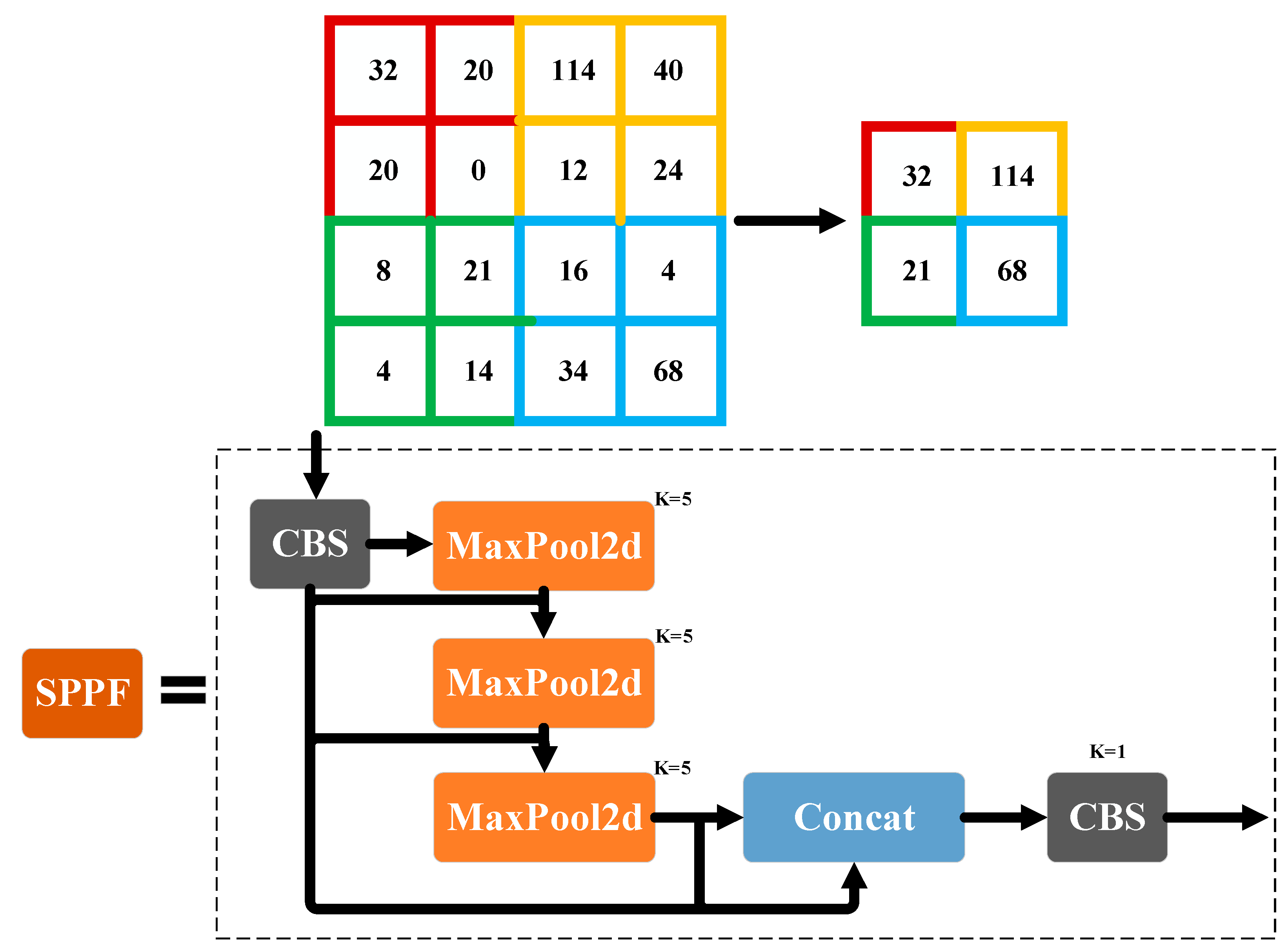
As shown in Figure 3, the Superfast Spatial Pyramid Pooling (SPPF) module employs multi-scale pooling operations (1 × 1, 5 × 5, 9 × 9, 13 × 13) [23], expanding the receptive field while maintaining computational efficiency and improving adaptability to defects of varying sizes. Furthermore, a C2PSA module is added after SPPF to further enhance feature extraction capabilities. Concurrently, FFNs map input features to higher-dimensional spaces, capturing complex nonlinear relationships within the input features, enabling the model to learn richer feature representations.

The Cross-Stage Partial Pyramid Slicing Attention (C2PSA) mechanism incorporates a multi-head attention (PSA) layer [24] into the C2f architecture. This efficient local self-attention module feeds a portion of convolutional features into a module comprising a multi-head self-attention (MHSA) and a feedforward network (FFN). The network structure diagram is shown in Figure 4, the two components are then concatenated and fused through convolution, enhancing feature representation in critical regions. Furthermore, weighting feature maps through the self-attention mechanism allows focusing on critical region features while suppressing interference from irrelevant background information (e.g., ballast, debris around rails).

2.2. Neck Network (Neck)

The Neck Network enhances the correlation of multi-scale features through feature fusion. It comprises Upsample, Concat, and C3k2 modules [25], where the Upsample operation scales high-resolution feature maps to match low-resolution ones, enabling the fusion of shallow-level detail features with deep-level semantic features. The concatenation operation (Concat) then combines feature maps of different scales along the channel dimension, preserving multi-scale feature information and improving the detection capability for small object defects.

Finally, the Neck network section also employs C3k2 modules to aggregate multiscale features and optimize their propagation. Additionally, CARAFE content-aware upsampling replaces conventional bilinear interpolation, improving detail retention by 25%. EVC (Enhanced Visual Centering) concentrates on core regions, boosting accuracy by 2.5% in complex scenes. Further strengthening the fused features, cross-layer connections enhance feature flow, providing high-quality feature inputs for subsequent detection heads. Inter-layer connections further reinforce feature fusion and improve feature flow, delivering high-quality feature inputs for subsequent detection heads.

2.3. Detection Head (Head)

YOLO11 employs multi-scale prediction heads to detect objects of varying sizes. The backbone and neck generate detection boxes at three distinct scales, projecting predictions onto three feature maps: P3 (8 × 8), P4 (16 × 16), and P5 (32 × 32). This ensures comprehensive coverage of diverse defect types [26]. Unlike YOLO8, the cls branch employs Deep-Separable Convolution (DWConv) for lightweight outputs, enhancing computational efficiency. The detection head design draws inspiration from YOLO11 by utilizing two prediction heads: one with one-to-many assignment and the other with one-to-one assignment. This dual-head architecture’s assignment strategy effectively boosts the model’s detection performance.

3. Improvement Strategies and Outcomes

3.1. Adaptive Downsampling Method (ADown)

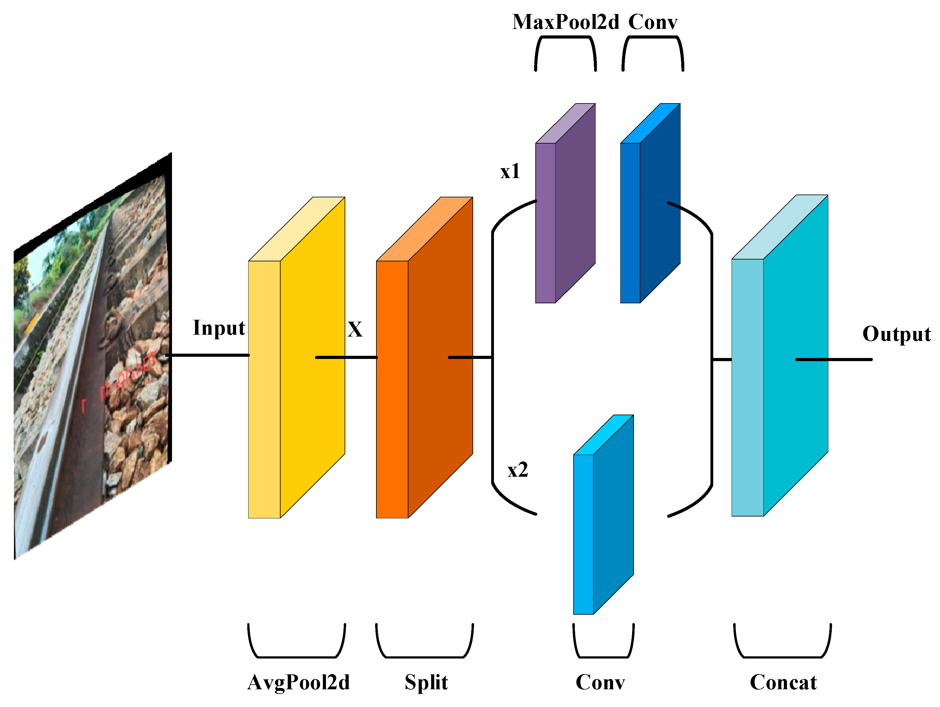
The original YOLO11 backbone network employs standard convolution downsampling to adjust feature map dimensions by controlling stride size. However, this approach significantly reduces feature map resolution and causes fine textures and edge information of small objects to be more easily lost. Therefore, to effectively enhance the model’s feature perception capability for rail defects, this experiment replaces the Conv module with the Adaptive Downsampling (ADown) method proposed in YOLO9. As shown in the workflow diagram in Figure 5, the feature map first undergoes 2D average pooling (AvgPool2d) [27] to preserve complete global features. For detailed feature detection, the feature map is then split into two sub-feature maps along the channel dimension. One sub-feature map undergoes direct downsampling through a convolutional layer for feature detection. The other sub-feature map first passes through a 2D max pooling layer (MaxPool2d) to extract the maximum value within the pooling window, highlighting prominent image features. This sub-feature map is then downsampled to extract local features. ADown balances the efficiency of downsampling and the preservation of fine-grained features through “multi-path feature processing”. For the input feature map $X\in R^{C\times H\times W}$ (where C denotes the number of channels, H the height, and W the width), a 2 × 2 average pooling (AvgPool2d) with a stride of 2 is applied to generate the global feature map $X_{avg}\in R^{C\times {\displaystyle \frac{H}{2}}\times {\displaystyle \frac{W}{2}}}$, which avoids the loss of global semantics and thus achieves global feature preservation. The original feature map $X$ is split into two subgraphs $X_1\in R^{{\displaystyle \frac{C}{2}}\times H\times W}$ and $X_2\in R^{{\displaystyle \frac{C}{2}}\times H\times W}$ at a 1:1 ratio along the channel dimension. Among them, Branch 1 (direct downsampling): $X_1$ is processed by a standard 3 × 3 convolution (Conv2d, stride = 2, padding = 1) to generate the local feature $X_{1_{conv}}$: Branch 2 (local salient feature enhancement): $X_2$ first undergoes 2 × 2 max pooling (MaxPool2d, stride = 2) to extract prominent edges and textures, and then is processed by a convolution of the same specification to generate $X_{2_{pool-conv}}$, realizing channel splitting and branch processing. The final downsampled feature is output by concatenation (Concat) along the channel dimension; although the number of channels increases, it is compressed by subsequent modules, which does not add excessive computational overhead and achieves the effect of feature fusion. Its calculation formulas are shown in Equations (5)–(9).

$$\mathrm{G}\mathrm{l}\mathrm{o}\mathrm{b}\mathrm{a}\mathrm{l} \mathrm{F}\mathrm{e}\mathrm{a}\mathrm{t}\mathrm{u}\mathrm{r}\mathrm{e} \mathrm{E}\mathrm{x}\mathrm{t}\mathrm{r}\mathrm{a}\mathrm{c}\mathrm{t}\mathrm{i}\mathrm{o}\mathrm{n} X_{avg}=AvgPool2d(X,kernel=2,stride=2)$$

(5)

$$\mathrm{C}\mathrm{h}\mathrm{a}\mathrm{n}\mathrm{n}\mathrm{e}\mathrm{l} \mathrm{S}\mathrm{p}\mathrm{l}\mathrm{i}\mathrm{t}\mathrm{t}\mathrm{i}\mathrm{n}\mathrm{g} X_1,X_2=Split(X,dim=1,ratio=0.5)$$

(6)

$$\mathrm{B}\mathrm{r}\mathrm{a}\mathrm{n}\mathrm{c}\mathrm{h} 1 \mathrm{P}\mathrm{r}\mathrm{o}\mathrm{c}\mathrm{e}\mathrm{s}\mathrm{s}\mathrm{i}\mathrm{n}\mathrm{g} X_{1_{conv}}=Conv2d(X_1,kernel=3,stride=2,padding=1)$$

(7)

$$\mathrm{B}\mathrm{r}\mathrm{a}\mathrm{n}\mathrm{c}\mathrm{h} 2 \mathrm{P}\mathrm{r}\mathrm{o}\mathrm{c}\mathrm{e}\mathrm{s}\mathrm{s}\mathrm{i}\mathrm{n}\mathrm{g} \left\{\begin{array}{c}{X}_{2_{conv}}=MaxPool2d(X_2,kernel=2,stride=2)\\ X_{2_{pool-conv}}=Conv2d(X_{2_{pool}},kernel=3,stride=1,padding=1)\end{array}\right.$$

(8)

$$\mathrm{f}\mathrm{e}\mathrm{a}\mathrm{t}\mathrm{u}\mathrm{r}\mathrm{e} \mathrm{f}\mathrm{u}\mathrm{s}\mathrm{i}\mathrm{o}\mathrm{n} X_{ADown}=Concat(X_{avg},X_{1_{conv}},X_{2_{pool-conv}},dim=1)$$

(9)

3.2. Design of SOEP-RFPN-MFM for Neck Network

The paper’s improvement logic aims to innovate upon the original Small Object Enhancement Pyramid (SOEP) module by integrating the Spatial-Normalization Interaction (SNI) module from the ECCV 2024 paper [28] “Rethinking FPN”, This method calculates the spatial mean/variance of each channel for the input features $\mathrm{F}\in R^{C\times H\times W}$ (instead of the batch mean of traditional Batch Normalization (BN)), avoiding the impact of batch fluctuations on small defect detection and achieving spatial normalization. To enhance spatial attention, a spatial attention matrix is generated via 1 × 1 convolution to weight the normalized features, highlighting defect regions and suppressing background interference. The weighted normalized features are residual-connected with the original features, which preserves the original details while ensuring semantic consistency to realize residual fusion, the mathematical representations are given by Equations (10)–(13).

$$\mathrm{S}\mathrm{p}\mathrm{a}\mathrm{t}\mathrm{i}\mathrm{a}\mathrm{l} \mathrm{M}\mathrm{e}\mathrm{a}\mathrm{n} \mathrm{C}\mathrm{a}\mathrm{l}\mathrm{c}\mathrm{u}\mathrm{l}\mathrm{a}\mathrm{t}\mathrm{i}\mathrm{o}\mathrm{n} {\mu }_s\left(c,h,w\right)={\displaystyle \frac{1}{H\times W}}\sum _{i=1}^H\sum _{j=1}^{W}F(c,i,j)$$

(10)

$$\mathrm{S}\mathrm{p}\mathrm{a}\mathrm{t}\mathrm{i}\mathrm{a}\mathrm{l} \mathrm{V}\mathrm{a}\mathrm{r}\mathrm{i}\mathrm{a}\mathrm{n}\mathrm{c}\mathrm{e} \mathrm{C}\mathrm{a}\mathrm{l}\mathrm{c}\mathrm{u}\mathrm{l}\mathrm{a}\mathrm{t}\mathrm{i}\mathrm{o}\mathrm{n} {\sigma }_S^2\left(c,h,w\right)={\displaystyle \frac{1}{H\times W}}\sum _{i=1}^H\sum _{j=1}^W(F\left(c,i,j\right)-{\mu }_s\left(c,h,w\right){)}^2$$

(11)

$$\mathrm{N}\mathrm{o}\mathrm{r}\mathrm{m}\mathrm{a}\mathrm{l}\mathrm{i}\mathrm{z}\mathrm{a}\mathrm{t}\mathrm{i}\mathrm{o}\mathrm{n} \mathrm{a}\mathrm{n}\mathrm{d} \mathrm{A}\mathrm{t}\mathrm{t}\mathrm{e}\mathrm{n}\mathrm{t}\mathrm{i}\mathrm{o}\mathrm{n} \mathrm{W}\mathrm{e}\mathrm{i}\mathrm{g}\mathrm{h}\mathrm{t}\mathrm{i}\mathrm{n}\mathrm{g} \hat{F}={\displaystyle \frac{F-{\mu }_s}{\sqrt{{\sigma }_S^2+ϵ}}}·A+\beta$$

(12)

$$\mathrm{R}\mathrm{e}\mathrm{s}\mathrm{i}\mathrm{d}\mathrm{u}\mathrm{a}\mathrm{l} \mathrm{F}\mathrm{u}\mathrm{s}\mathrm{i}\mathrm{o}\mathrm{n} F_{SNI}=\alpha ·\widehat{F}+(1-\alpha )·F$$

(13)

GSConvE, this method reduces the computational cost through “convolution decomposition + weighted fusion” (reducing FLOPs by 40% compared with standard convolution) while preserving the local textures of tiny defects. First, Group Convolution (GConv) groups the input feature $F$ by channels (with the number of groups $g={\displaystyle \frac{C}{2}}$, and each group independently performs 3 × 3 convolution to reduce parameter redundancy. Second, Depthwise Separable Convolution (DWConv) is applied to the input feature $F$ for channel-wise 3 × 3 convolution, focusing on extracting local details. Finally, the results of GConv and DWConv are fused via learnable weights to complete weighted fusion, balancing global semantics and local details. Its mathematical expressions are given by Equations (14)–(16).

$$\mathrm{G}\mathrm{C}\mathrm{o}\mathrm{n}\mathrm{v} F_{GConv}=GroupConv(F,groups=g,kernel=3,stride=1,padding=1)$$

(14)

$$\mathrm{D}\mathrm{W}\mathrm{C}\mathrm{o}\mathrm{n}\mathrm{v} F_{DWConv}=DepthWiseConv(F,groups=g,kernel=3,stride=1,padding=1)$$

(15)

$$\mathrm{W}\mathrm{e}\mathrm{i}\mathrm{g}\mathrm{h}\mathrm{t}\mathrm{e}\mathrm{d} \mathrm{F}\mathrm{u}\mathrm{s}\mathrm{i}\mathrm{o}\mathrm{n} F_{GSConvE}=\gamma ·F_{GConv}+(1-\gamma )·F_{DWConv}$$

(16)

The Multiscale Feature Modulation (MFM) module from the CVPR 2024 paper [29] “DCMPNet”, it receives the three-scale features from the neck network (P3: $F_3\in R^{C3\times H3\times W3}$, P4: $F_4$, P5: $F_5$). Then, Global Average Pooling (GAP) is performed on each scale feature to extract channel-level feature vectors. Through fully connected layers (FC) plus Sigmoid activation, dynamic weights $w_3,w_4,w_5$ for each scale are generated (with the weight range of [0, 1], where the weights corresponding to small target features are higher). Finally, the weights are used to weight the features of each scale, bilinear interpolation is adopted to unify the dimensions, and the fused features $F_{MFM}$ are output by summation. Its mathematical expressions are given by Equations (17)–(20).

$$\mathrm{G}\mathrm{A}\mathrm{P} {\mathrm{v}}_{\mathrm{k}}=\mathrm{G}\mathrm{A}\mathrm{P}\left({\mathrm{F}}_{\mathrm{k}}\right)={\displaystyle \frac{1}{{\mathrm{H}}_{\mathrm{k}}\times {\mathrm{W}}_{\mathrm{k}}}}\sum _{\mathrm{i}=1}^{{\mathrm{H}}_{\mathrm{k}}}\sum _{\mathrm{j}=1}^{{\mathrm{W}}_{\mathrm{k}}}{\mathrm{F}}_{\mathrm{k}}(\mathrm{i},\mathrm{j})(\mathrm{k}=3,4,5)$$

(17)

$$\mathrm{D}\mathrm{y}\mathrm{n}\mathrm{a}\mathrm{m}\mathrm{i}\mathrm{c} \mathrm{W}\mathrm{e}\mathrm{i}\mathrm{g}\mathrm{h}\mathrm{t} \mathrm{G}\mathrm{e}\mathrm{n}\mathrm{e}\mathrm{r}\mathrm{a}\mathrm{t}\mathrm{i}\mathrm{o}\mathrm{n} {\mathrm{w}}_{\mathrm{k}}=\mathsf{\sigma }\left(\mathrm{F}\mathrm{C}\left({\mathrm{v}}_{\mathrm{k}},\mathrm{o}\mathrm{u}{\mathrm{t}}_{\mathrm{d}\mathrm{i}\mathrm{m}}=1\right)\right)=\mathsf{\sigma }(\mathrm{W}·{\mathrm{v}}_{\mathrm{k}}+\mathrm{b})$$

(18)

$$\mathrm{S}\mathrm{c}\mathrm{a}\mathrm{l}\mathrm{e} \mathrm{W}\mathrm{e}\mathrm{i}\mathrm{g}\mathrm{h}\mathrm{t}\mathrm{i}\mathrm{n}\mathrm{g} {\widehat{\mathrm{F}}}_{\mathrm{k}}={\mathrm{w}}_{\mathrm{k}}·{\mathrm{F}}_{\mathrm{k}}$$

(19)

$$\mathrm{D}\mathrm{i}\mathrm{m}\mathrm{e}\mathrm{n}\mathrm{s}\mathrm{i}\mathrm{o}\mathrm{n} \mathrm{U}\mathrm{n}\mathrm{i}\mathrm{f}\mathrm{i}\mathrm{c}\mathrm{a}\mathrm{t}\mathrm{i}\mathrm{o}\mathrm{n} \mathrm{a}\mathrm{n}\mathrm{d} \mathrm{F}\mathrm{u}\mathrm{s}\mathrm{i}\mathrm{o}\mathrm{n} {\mathrm{F}}_{\mathrm{M}\mathrm{F}\mathrm{M}}=\mathrm{U}\mathrm{p}\mathrm{s}\mathrm{a}\mathrm{m}\mathrm{p}\mathrm{l}\mathrm{e}\left({\widehat{\mathrm{F}}}_5,\mathrm{s}\mathrm{i}\mathrm{z}\mathrm{e}=\mathrm{H}3\right)+\mathrm{U}\mathrm{p}\mathrm{s}\mathrm{a}\mathrm{m}\mathrm{p}\mathrm{l}\mathrm{e}\left({\widehat{\mathrm{F}}}_{4,}\mathrm{s}\mathrm{i}\mathrm{z}\mathrm{e}=\mathrm{H}3\right)-{\widehat{\mathrm{F}}}_3$$

(20)

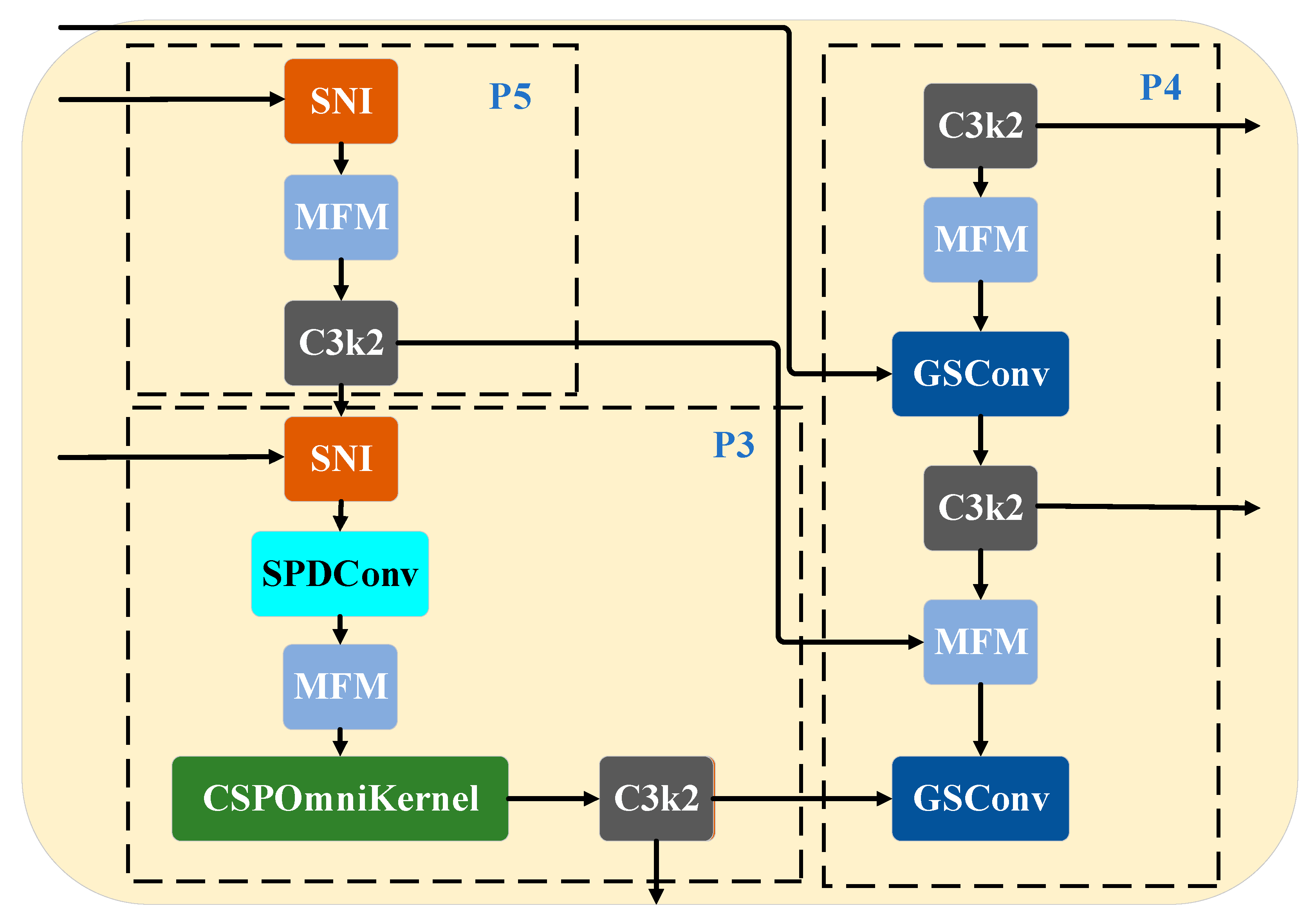
This ultimately achieves further optimization of small object detection performance. Its network architecture is illustrated in Figure 6.

For P5 feature processing (large object detection layer), the SNI module is applied to the input features. This optimizes the spatial normalization interaction logic, reduces semantic bias during multi-scale feature fusion, and enhances feature consistency. The output is then fused with the P4 features from the backbone. The MFM module performs multiscale feature modulation, using dynamic weight allocation to strengthen the finegrained features corresponding to small objects. Finally, the output is processed through two C3k2 modules.

For P3 feature processing (small object detection layer), the SNI module is similarly applied. However, SPDConv downsampling is used on the backbone’s P3 features to extract features containing small object information. SPDConv avoids the loss of small defect information during downsampling through “patch splitting + local convolution”, and the process is as follows: it splits the input feature $\mathrm{F}\in R^{C\times H\times W}$ into non-overlapping 2 × 2 patches, with each patch having a size of c × 2 × 2 (where c stands for the number of channels), thus achieving patch splitting; it performs 3 × 3 convolution on each patch individually (with a stride of 2 and padding of 1), completes downsampling inside the patch and preserves local details, thereby realizing downsampling via local convolution; finally, it reconcatenates the convolved patches to restore the complete feature map $F_{SPDConv}$. Its mathematical formulas are given by Equations (21)–(23).

$$\mathrm{P}\mathrm{a}\mathrm{t}\mathrm{c}\mathrm{h} \mathrm{S}\mathrm{p}\mathrm{l}\mathrm{i}\mathrm{t}\mathrm{t}\mathrm{i}\mathrm{n}\mathrm{g} {\mathrm{F}}_{\mathrm{p}\mathrm{a}\mathrm{t}\mathrm{c}\mathrm{h}}=\mathrm{P}\mathrm{a}\mathrm{t}\mathrm{c}\mathrm{h}\mathrm{S}\mathrm{o}\mathrm{l}\mathrm{i}\mathrm{t}(\mathrm{F},\mathrm{p}\mathrm{a}\mathrm{t}\mathrm{c}{\mathrm{h}}_{\mathrm{s}\mathrm{i}\mathrm{z}\mathrm{e}}=2,\mathrm{o}\mathrm{v}\mathrm{e}\mathrm{r}\mathrm{l}\mathrm{a}\mathrm{p}+0)$$

(21)

$$\mathrm{L}\mathrm{o}\mathrm{c}\mathrm{a}\mathrm{l} \mathrm{C}\mathrm{o}\mathrm{n}\mathrm{v}\mathrm{o}\mathrm{l}\mathrm{u}\mathrm{t}\mathrm{i}\mathrm{o}\mathrm{n} {\mathrm{F}}_{\mathrm{p}\mathrm{a}\mathrm{t}\mathrm{c}\mathrm{h}\_\mathrm{c}\mathrm{o}\mathrm{n}\mathrm{v}}=\mathrm{C}\mathrm{o}\mathrm{n}\mathrm{v}2\mathrm{d}({\mathrm{F}}_{\mathrm{p}\mathrm{a}\mathrm{t}\mathrm{c}\mathrm{h}},\mathrm{k}\mathrm{e}\mathrm{r}\mathrm{n}\mathrm{e}\mathrm{l}=3,\mathrm{s}\mathrm{t}\mathrm{r}\mathrm{i}\mathrm{d}\mathrm{e}=2,\mathrm{p}\mathrm{a}\mathrm{d}\mathrm{d}\mathrm{i}\mathrm{n}\mathrm{g}=1)$$

(22)

$$\mathrm{P}\mathrm{a}\mathrm{t}\mathrm{c}\mathrm{h} \mathrm{C}\mathrm{o}\mathrm{n}\mathrm{c}\mathrm{a}\mathrm{t}\mathrm{e}\mathrm{n}\mathrm{a}\mathrm{t}\mathrm{i}\mathrm{o}\mathrm{n} {\mathrm{F}}_{\mathrm{S}\mathrm{P}\mathrm{D}\mathrm{C}\mathrm{o}\mathrm{n}\mathrm{c}}=\mathrm{P}\mathrm{a}\mathrm{t}\mathrm{c}\mathrm{h}\mathrm{M}\mathrm{e}\mathrm{r}\mathrm{g}\mathrm{e}({\mathrm{F}}_{\mathrm{p}\mathrm{a}\mathrm{t}\mathrm{c}{\mathrm{h}}_{\mathrm{c}\mathrm{o}\mathrm{n}\mathrm{v}}},\mathrm{o}\mathrm{r}\mathrm{i}\mathrm{g}\mathrm{i}\mathrm{n}\mathrm{a}{\mathrm{l}}_{\mathrm{s}\mathrm{i}\mathrm{z}\mathrm{e}}=({\displaystyle \frac{\mathrm{H}}{2}},{\displaystyle \frac{\mathrm{W}}{2}}))$$

(23)

Second, the SPDConv output, SNI results, and backbone P3 features are fused through the MFM module. This fusion undergoes multiscale feature integration via the CSPOmniKernel—a feature integration module designed based on the CSP architecture and OmniKernel. Finally, the output is processed by two C3k2 modules.

For P4 feature processing (medium object detection layer), the GSConvE module is selected. This reduces computational load while preserving more local detail features and adapting to small object edges and texture information acquisition. Subsequently, its output is similarly fused with the P4 features from the Head section via the MFM module, then processed through two C3k2 modules for output.

To enhance small object detection while maintaining computational efficiency and high detection accuracy, the paper introduces an additional P5 feature processing stage after P4. This stage reapplies the GSConvE module to balance efficiency and performance, followed by dynamic feature weight adjustment via the MFM module. The output is then fused with P5 features from the Head layer and processed through two C3k2 modules.

3.3. Module Synergistic Mechanism

The “Adown + SOEP-RFPN-MFM” combination is not merely a modular overlay, but a closed-loop system developed to meet the core demand of rail defect detection: “preserving fine-grained features first, then fusing and exploiting them efficiently”. Its functional complementarity directly targets the two key pain points of the original YOLO11n pointed out in the original manuscript.

As can be seen from the table, the core function of ADown is to “provide high-quality feature input”, it addresses the issue of “small defect feature loss” through multi-path processing, laying a foundation for subsequent fusion modules. The core function of SOEP-RFPN-MFM is to “utilize features efficiently”—it resolves the problems of “inefficient feature fusion and category confusion” through the collaboration of three sub-modules, converting the fine-grained features preserved by ADown into an improvement in detection accuracy. The two form a dependent relationship where “without ADown, the fusion module has no valid features to fuse, and without SOEP-RFPN-MFM, the preserved features cannot be adapted to the detection task”, which constitutes the optimal functional combination for rail defect detection rather than a simple stack of modules.

Combined with Figure 5 (ADown Workflow Diagram) and Figure 6 (SOEP-RFPN-MFM Network Architecture Diagram) in the original paper, the synergistic logic can be further verified: the feature maps output by ADown (including the edge textures of micro-cracks) are directly used as the P3/P4/P5 feature inputs for SOEP-RFPN-MFM. Among them, the P3 layer (small target detection layer) optimizes spatial normalization via the SNI module, and then the MFM module enhances the feature weights of small defects—this process clearly reflects the progressive relationship of “preservation first, optimization second, and enhancement last”, rather than the disordered stacking of modules.

4. Experimental Results and Analysis

4.1. Datasets and Experimental Environment

4.1.1. Rail Defect Dataset

To ensure that no confusion or overlap occurs among multiple data subsets in this experiment, the dataset used in this paper was collected from a single track line of a high-speed railway trunk line in China, covering railway rails under common environmental conditions. It includes four types of defects: Spalling (1506), Squat (1710), Wheel Burn (474), and Corrugation (987). The dataset comprises 4020 images with a resolution of 640 × 640, divided into training and validation sets at a ratio of approximately 4:1. Annotation was performed using the LabelImg 1.8.6 tool, with bounding boxes marking defect regions and labels formatted in YOLO (.txt) format. The minimum step size for the precision requirement of annotation boxes is set to 1 pixel (corresponding to an actual size of approximately 0.1 mm, which meets the annotation requirements for micro-cracks smaller than 0.2 mm), so as to avoid the offset of annotation boxes for small defects caused by an excessively large step size. A three-step annotation process of “Initial Annotation–Review–Final Approval” is adopted:

• Initial Annotation: A single annotator draws annotation boxes for defect areas and fills in the defect categories (Spalling/Squat/Wheel Burn/Corrugation) as well as the defect dimensions;
• Review: Another annotator inspects the initial annotation results image by image, with a focus on verifying the integrity of annotation boxes for small defects (whether the entire defect area is covered) and the accuracy of defect categories;
• Inter-annotator Agreement Verification: Cohen’s Kappa coefficient was calculated to evaluate defect category consistency (Kappa = 0.89, indicating high agreement), and IoU (Intersection over Union) was used to measure bounding box overlap consistency (average IoU = 0.91 for all defects, ≥0.85 for small defects);
• Final Approval: A senior instructor resolves disputed annotations identified in the review stage and generates the final annotation files (YOLO-format .txt files containing annotation box coordinates and category IDs).

4.1.2. Experimental Environment

The experimental environment for this article uses the Windows 10 operating system. The hardware configuration includes a 12th Gen Intel (R) Core (TM) i5-124007 CPU (2.50 GHz), an NVIDIA GeForce RTX 4060 graphics card, and 8 GB of RAM. Software components include Python 3.11.9, the Ultralytics YOLO framework, Pytorch 2.7.1 + cu118, and CUDA 11.8. Model training parameters are detailed in

Table 1. Functional Synergistic Logic and Pain Point Matchings.

Module	Core Function	Addressed Rail Detection Pain Points
ADown	Two-dimensional average pooling preserves the global features of steel rails. Channel-wise processing of feature maps: one branch for convolutional downsampling and one branch for MaxPool to extract local details	Standard convolutional downsampling in the original model causes the loss of texture information for <0.2 mm micro-cracks and micro-spalling.
SOEP-RFPN-MFM	SNI Module: Optimizes spatial normalization interaction and reduces the semantic deviation between ballast background and defects. GSConvE Module: Uses lightweight convolution to balance the computational cost and the preservation of strip texture for wheel burn. MFM Module: Implements dynamic weight assignment and enhances the feature representation of small defects smaller than 50 pixels2.	Features of large targets mask the features of small defects. Due to similar textures, wheel burn and corrugated wear exhibit a high inter-class confusion rate.

. Additional information on the model’s training phase is available in

Table 2. Model Training Parameters.

Project	Parameter Value or Name
CPU	12th Gen Intel (R) Core (TM) i5-124007 (2.50 GHz)
GPU	NVIDIA GeForce RTX 4060
Operating system	Windows 11
Programming language	Python 3.11.9
Deep learning framework	Pytorch 2.7.1
CUDA	11.8
Training Iterations	300

. An optimizer with strong anti-background interference capability (SGD) combined with a momentum of 0.937 is adopted to stabilize gradient updates and avoid parameter oscillation caused by abnormal samples. A batch size of 64 that is more compatible with the RTX 4060 is selected, and the learning rate (0.01), weight decay (0.0005), and image size (640 × 640) are set to achieve three objectives: matching the pre-trained weights of SGD and YOLO11n, balancing the trade-off between “suppressing overfitting” and “preserving small defect features”, and retaining the detailed characteristics of small defects. Additional information on the model’s training phase is available in

Table 3. Model hyperparameter settings.

Parameters	Setup
Batch size	64
Image size	640 × 640
Initial learning rate	0.01
Final learning rate	0.01
Weight decay	0.0005
Momentum	0.937
Optimizer	SGD

.

4.1.3. Evaluation Metrics

To effectively evaluate the improved YOLO11n model, the paper employs four evaluation metrics: Precision (P), Recall (R), Mean Average Precision (mAP), and F1 score. Precision measures the proportion of predicted “positive samples” (detected objects) that are actually true positives (TP), indicating the model’s ability to reduce false positives. Recall measures the proportion of all actual positive samples successfully detected by the model (TP), reflecting its capability to minimize false negatives. Multi-class Mean Average Precision (mAP) is a core metric for evaluating multi-class object detection models. It is calculated by averaging the AP values across all classes. The F1 score is the harmonic mean of Precision and Recall, providing a balanced assessment that avoids the limitations of relying on a single metric. The specific calculations are shown in Formulas (24)–(27).

$$\mathrm{P}={\displaystyle \frac{TP}{TP+FP}}$$

(24)

$$\mathrm{R}={\displaystyle \frac{TP}{TP+FN}}$$

(25)

$$\mathrm{m}\mathrm{A}\mathrm{P}={\displaystyle \frac{1}{\left|N\right|}}\sum _{n\in N}{AP}_n$$

(26)

$$\mathrm{F}1=2·{\displaystyle \frac{P·R}{P+R}}$$

(27)

In the above formula, TP (True Positive) refers to a predicted target belonging to a certain class that is indeed of that class, with the intersection-over-union (IoU) between the detection bounding box and the ground truth bounding box meeting the set threshold. FP (False Positive) occurs under either of the following conditions:

• A target is predicted to belong to a certain class but does not actually exist in that class;
• The predicted class is incorrect;
• The predicted class is correct, but the IoU < falls below the threshold.

AP denotes the area under the P-R (Precision–Recall) curve, while mAP represents the 230 average of the average precision (AP) across all classes.

4.2. Ablation Studie

To validate the effectiveness of the improvement strategy for YOLO11, a progressive ablation experiment was designed. The results are shown in Table 2.

Table 4. Comparison of Experimental Models with Different Module Combinations.

Algorithm Configuration	Precision (P)	Recall (R)	Mean Average Precision (mAP)	F1 Score
YOLO11n	92.5%	89.6%	94.8%	91.2%
+ADown	96%	93.4%	97.6%	95%
+SOEP-RFPN-MFM	93.6%	87.9%	95.2%	91%
+SOEP-RFPN-MFM + Original Downsampling	93.5%	87.7%	95.0%	90.8%
+ADown + SOEP-RFPN-MFM without the MFM module	93.2%	90.5%	94.5%	91.8%
+ADown+SOEP-RFPN-MFM	93.7%	92.4%	95.6%	93%

data indicates that the original YOLO11n achieved a precision of 92.5%, a recall of 89.6%, a mean average precision (mAP) of 94.8%, and an F1 score of 91.2%. Both improvement methods—replacing the backbone network with ADown and replacing the neck network with the SOEP-RFPN-MFM module—showed performance gains over the original YOLO11n across all metrics. Secondly, two sets of auxiliary experiments were conducted, namely + SOEP-RFPN-MFM + Original Downsampling and +ADown + SOEP-RFPN-MFM without the MFM module, and the performance results of both showed a decline. The reason is that when only SOEP-RFPN-MFM is added, the neck module will excessively focus on the redundant features of the rail background in the absence of sufficient fine-grained features, leading to a reduction in the distinguishability between defect features and background features. Additionally, although the GSConvE submodule of SOEP-RFPN-MFM is lightweight, it increases the number of computation steps by 2 compared with the original neck module, resulting in an alignment deviation of 1–2 pixels in the feature map during the upsampling and downsampling processes. This thus demonstrates that only the combination of +ADown + SOEP-RFPN-MFM can achieve a synergistic improvement in precision, recall, and mAP. This demonstrates that both the ADown module and SOEP-RFPN-MFM effectively enhance the accuracy of rail defect detection. However, to better adapt the model to processing minute feature information in complex environments, both methods were combined and trained together. Finally, comparison with the original YOLO11n reveals significant improvements: precision (P) increased by 1.2 percentage points, recall (R) rose by 2.6 percentage points, mean average precision (mAP) improved by 0.8 percentage points, and F1 score increased by 1.8 percentage point.

4.3. Comparative Experiments with Mainstream Models

The improved algorithm was compared with Faster R-CNN, SSD, RT-DETR-tiny, YOLOv5, YOLOv8, YOLOv10n, and the original YOLO11n from the YOLO series on the track defect dataset. The results are shown in

Table 5. Experimental Model vs. Mainstream Model Comparison Results.

Model	Precision (P)	Recall (R)	Mean Average Precision (mAP)	F1 Score
Faster R-CNN	93.0%	88.5%	94.0%	90.7%
SSD	91.5%	87.2%	93.5%	89.3%
YOLOv5	93.2%	91.1%	95%	92%
YOLOv8	93.4%	92.0%	95.3%	92.7%
YOLOv10n	84.5%	88.5%	93.6%	86%
YOLO11n	92.5%	89.6%	94.8%	91.2%
Improved YOLO11n	93.7%	92.4%	95.6%	93%
RT-DETR-tiny	93.5%	92.2%	95.4%	92.8%

.

As shown in the Table 5 above, the improved YOLO11n achieved the best performance with an accuracy rate of 93.7%, slightly higher than YOLOv8 (93.4%) and significantly higher than the original YOLO11n (92.5%) and YOLOv5 (93.2%), and substantially higher than YOLOv10n (84.5%). To highlight the improvement effects of the experiment in this study, by comparing the classic two-stage detector (Faster R-CNN), the early one-stage detector (the lightweight version of SSD), and RT-DETR-tiny from the recent DETR family, the improved YOLO11n outperforms all three in all metrics. This indicates the lowest proportion of non-defect samples misclassified as defects during trajectory defect prediction. Secondly, the improved YOLO11n achieves a recall rate of 92.4%, which is 0.4 percentage points higher than YOLOv8 (92.0%). Both significantly outperform the original YOLO11n (89.6%), YOLOv5 (91.1%), and YOLOv10n (88.5%). This demonstrates that the improved YOLO11n not only excels in controlling missed track defect samples but also surpasses YOLOv8 in recall performance, the improved YOLO11n achieves the best mAP at 95.6%, which is 0.3 percentage points higher than YOLOv8 (95.3%). This outperforms the original YOLO11n (94.8%), YOLOv5 (95%), and YOLOv10n (93.6%), indicating a significant improvement in comprehensive performance for track defect detection. Finally, the improved YOLO11n achieves the highest F1 score of 93%, which is 0.3 percentage points higher than YOLOv8 (92.7%). This outperformed the original YOLO11n (91.2%), YOLOv5 (92%), and YOLOv10n (86%), demonstrating equally outstanding performance in balancing precision and recall.

This

Table 6. Multi-dimensional Class-level AP Table.

Defect Types	Model Version	Class-Level AP@0.5 (Conventional Threshold)
Spalling	YOLO11n	93.7%
	Improved YOLO11n	94.2%
Squat	YOLO11n	97.6%
	Improved YOLO11n	98.2%
Wheel Burn	YOLO11n	91.4%
	Improved YOLO11n	91.4%
Corrugation	YOLO11n	98.5%
	Improved YOLO11n	98.5%

is a multi-dimensional class-level Average Precision (AP) table for rail defect detection, which primarily compares the class-level AP@0.5 detection accuracy of the basic YOLO11n model and the improved YOLO11n model for four types of rail defects at the conventional Intersection over Union (IoU) threshold of 0.5.

The data shows that the detection accuracy of different defect types exhibits differentiated performance: For spalling defects, the AP@0.5 of the basic model is 93.7%, and the improved version increases to 94.2%, with an increase of 0.5 percentage points; the detection accuracy of rail head internal defects shows a more significant improvement—the 97.6% value of the basic model reaches 98.2% after improvement, an increase of 0.6 percentage points. In contrast, the detection accuracy of two types of defects (wheel burn and corrugated wear) remains unchanged, with the AP@0.5 of the two models stably at 91.4% and 98.5%, respectively.

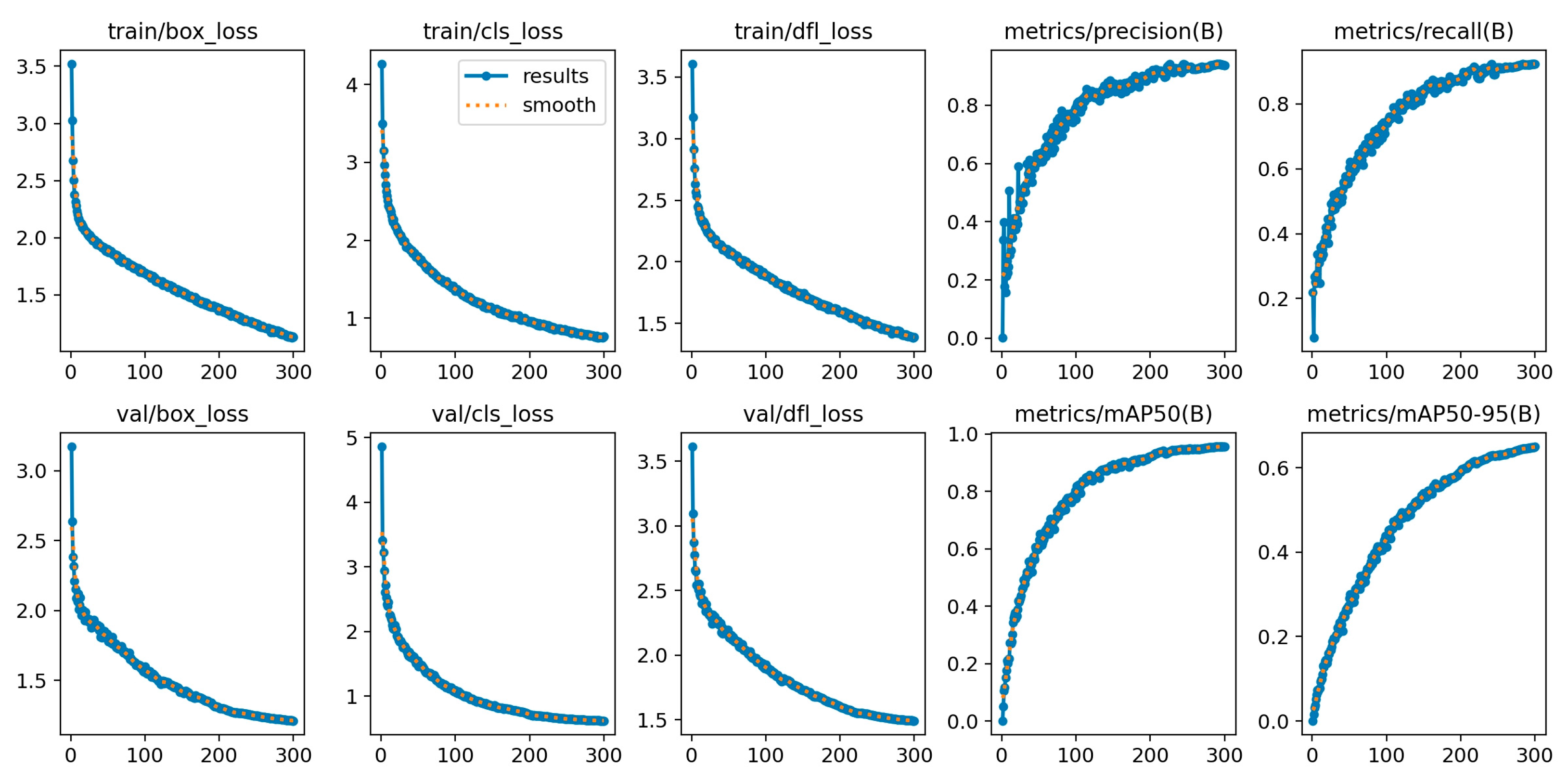
As can be seen from Figure 7, the first row shows the training loss curves. Among them, train/box_loss, train/cls_loss and train/dfl_loss all show a continuous downward trend, indicating that the prediction error of the model on the training set is constantly decreasing. The second row shows the validation loss curves. Val/box_loss, val/cls_loss and val/dfl_loss also decrease synchronously, and the trend is consistent with that of the training loss, indicating that the model does not show obvious over-fitting, and its generalization ability on the validation set is continuously improving. Secondly, both metrics/precision (B) and metrics/recall (B) show an upward trend and eventually stabilize, indicating that the “precision” and “recall” of the model for the target are continuously optimized. The metrics/mAP50 (B) curve rises significantly and finally approaches 1.0, a relatively loose matching threshold. The metrics/mAP50–95 (B) curve continues to rise, indicating that the detection performance of the model also improves steadily under a more stringent IoU threshold, and the model has a good degree of refinement in bounding box positioning.

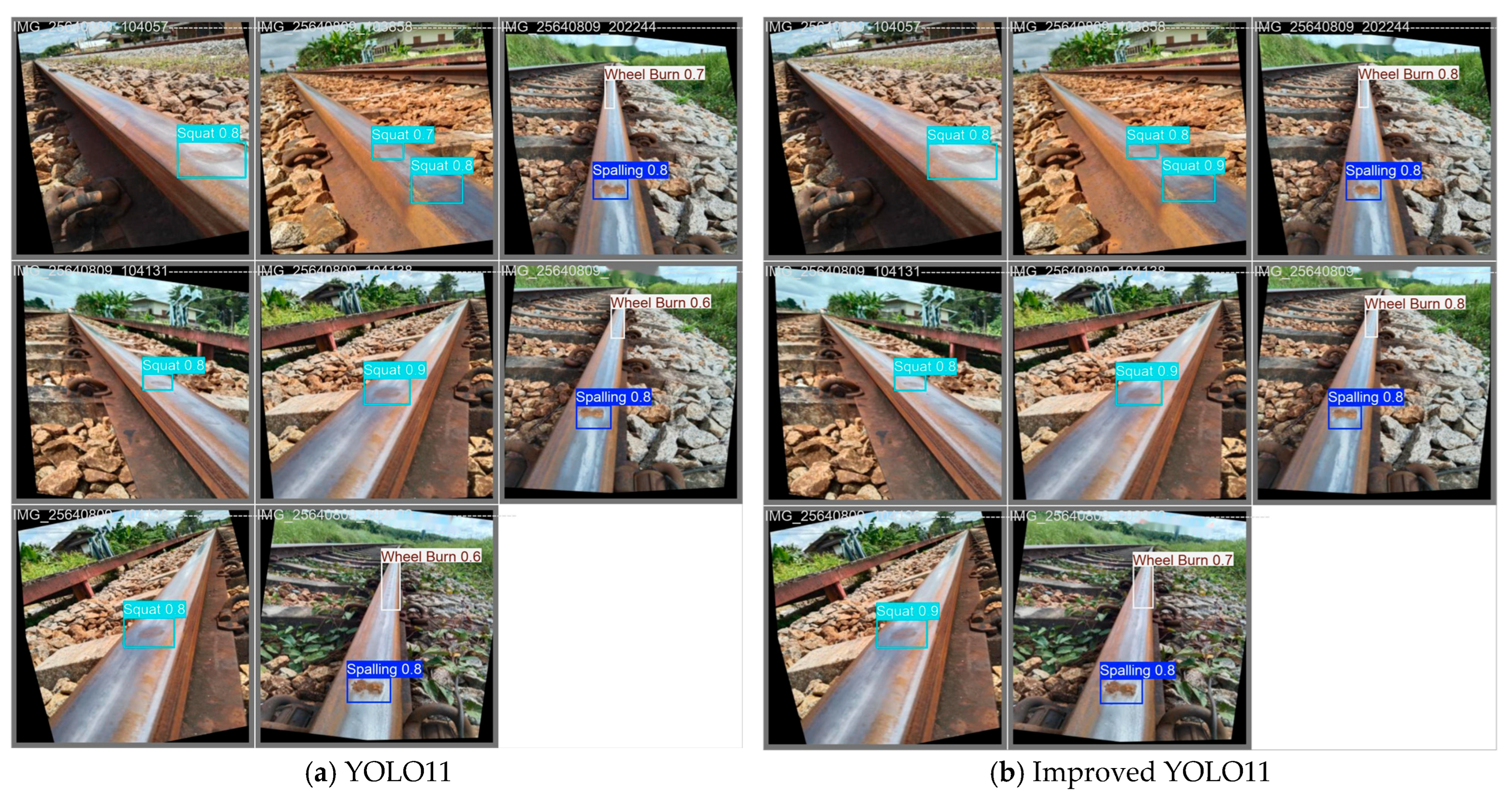
The comparison in Figure 8 shows that, in terms of the confidence metrics for Squat defects, the confidence levels of some detection results increased from “0.7” before modification to “0.8” or “0.9” after modification. For example, in the second image, “Squat 0.7” became “0.8”, and in the seventh image, “Squat 0.8” became “0.9”. For “Wheel Burn”-type defects, the original confidence levels of “0.6” and “0.7” increased to “0.8” and “0.7” after improvement. For instance, in the third image, “0.7” changed to “0.8”, and in the sixth image, “0.6” changed to “0.8‘. From the perspective of detection stability, the confidence levels of Squat defects were more concentrated around “0.8” and “0.9” after modification, indicating a reduction in fluctuations. Meanwhile, the confidence level of Spalling (rail spalling) defects remained at “0.8” in both types of images, demonstrating stable detection accuracy. At the same time, the improved model did not exhibit additional false positives or false negatives, indicating a significant optimization in the accuracy of rail defect detection, especially in the detection of low-confidence samples. This shows that the improved YOLO11 model has demonstrated remarkable improvements in terms of confidence, stability, and accuracy in rail defect detection, especially achieving significant optimization in the detection of Squat and Wheel Burn types of defects.

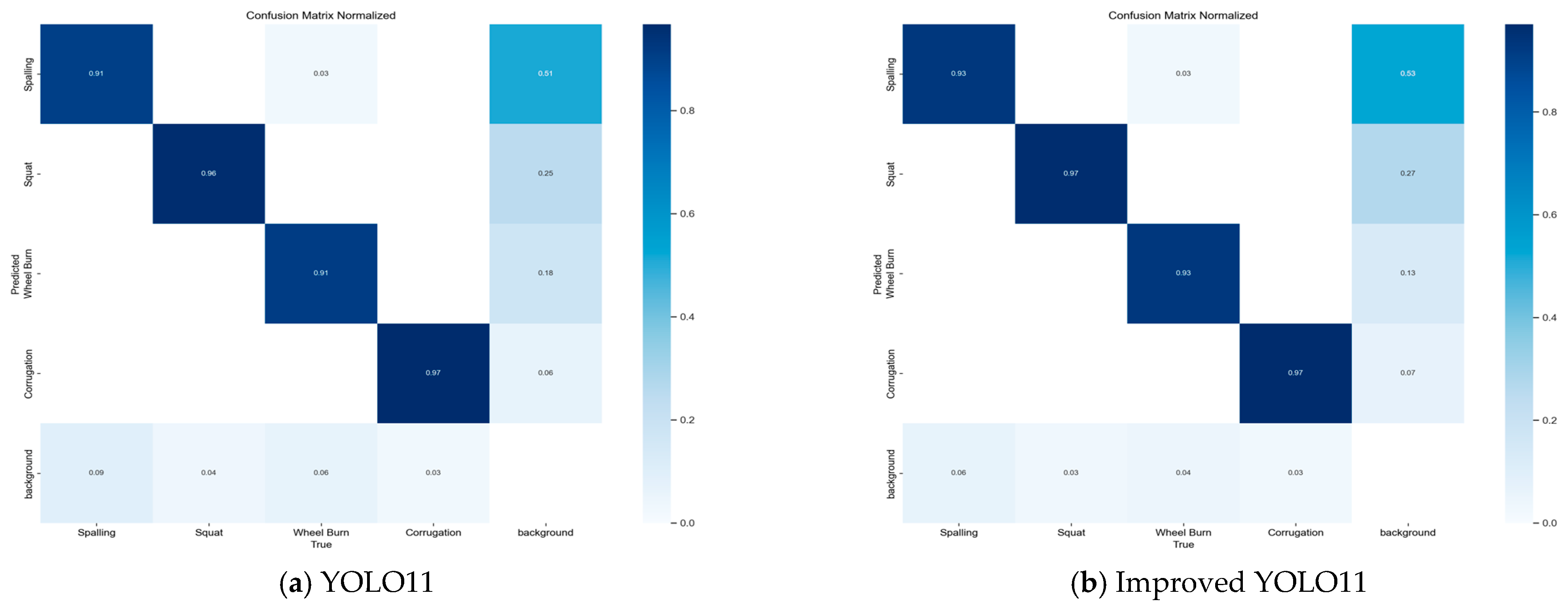
As can be seen from Figure 9, the core indicators on the diagonal of the matrix have all been optimized—spalling increased from 0.91 to 0.93, rail head internal defects rose from 0.96 to 0.97, and wheel burn went up from 0.91 to 0.93, with only corrugated wear maintaining a high level of 0.97. This indicates that the improved module has enhanced the discriminability of defect features, enabling more accurate identification of easily confused defects such as spalling and rail head internal defects. The values in the off-diagonal regions (inter-class misclassification) have decreased significantly; for example, the misclassification ratio corresponding to wheel burn dropped from 0.18 to 0.13, which reflects that the model’s ability to capture specific features such as the “color gradient of wheel burn discoloration” and “irregular edges of spalling” has been enhanced, effectively reducing the confusion among similar defects. The risk of background misjudgment (missed detection) has been reduced: the values in the bottom “background” row have generally decreased—the background misjudgment corresponding to spalling fell from 0.09 to 0.06, and that for rail head internal defects decreased from 0.04 to 0.03. This shows that the probability that the model misclassifies small defects as background has decreased, further shrinking the risk of missed detection.

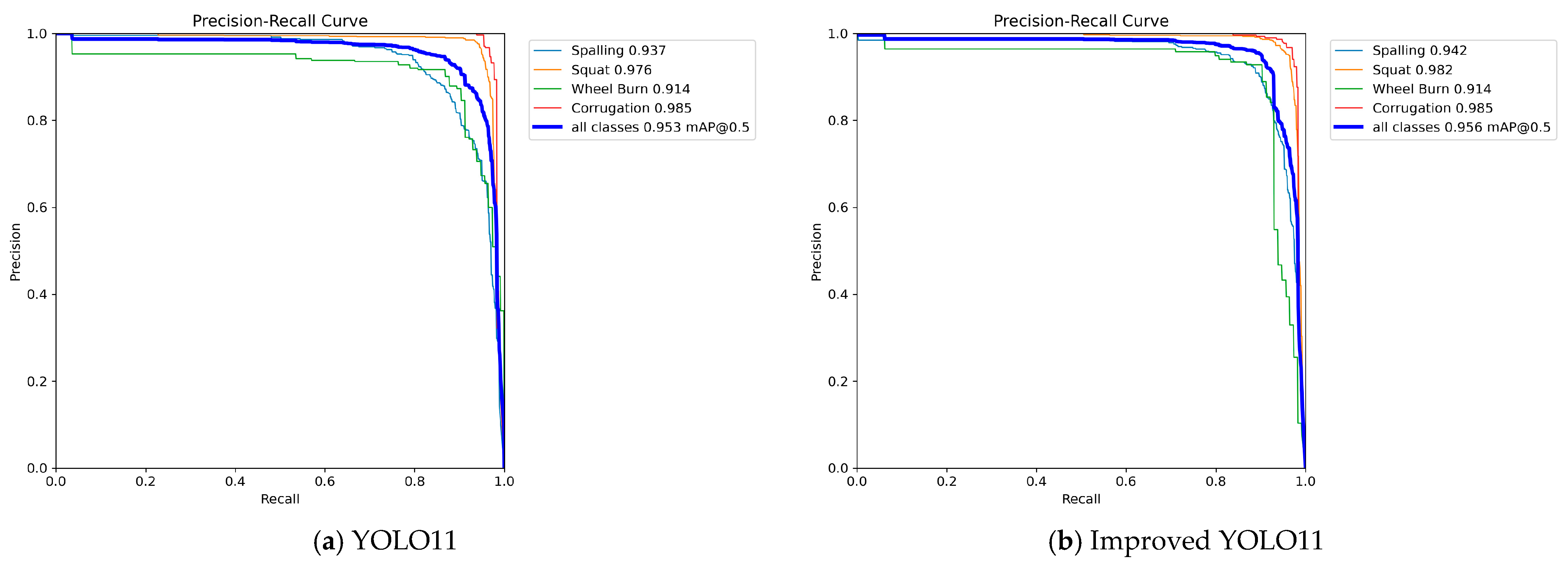
By comparing the Precision–Recall (P-R) curves of the YOLO11n model on the left and the improved YOLO11n model on the right in Figure 10, the Average Precision (AP) for single-class detection of Spalling and Squat defects has been optimized. The detection performance for Wheel Burn and Corrugation defects remains stable. In terms of the mean Average Precision (mAP), the mAP@0.5 of the original model across all categories is 0.953, which has increased to 0.956 after improvement. This indicates a significant enhancement in the overall performance of the model in the detection task. Regarding the shape of the curves and performance balance, the P-R curve of the improved model is more “upward and rightward”. This means that at the same recall rate, the precision is higher, or at the same precision rate, the recall rate is higher, suggesting better model performance. Additionally, in the high-recall region, the decline in precision is more gradual. This reflects a better balance between “precise detection” and “comprehensive coverage”, and also indicates a significant improvement in stability when identifying small-sample or hard-to-distinguish rail defects.

In summary, on the track defect dataset, the improved YOLO11n demonstrates overall superior performance compared to the original YOLO11n, YOLOv5, YOLOv8 and YOLOv10n. In terms of controlling false negatives for key defects, the system targets critical defects and increases the recall rate from 89.6% to 92.4% through the synergy of ADown and SOEP-RFPN-MFM. In the aspect of preventive maintenance optimization, the system achieves risk-stratified scheduling with stable defect confidence, effectively avoiding the exorbitant costs of emergency rail replacement. In conclusion, the improved model reaches a higher level of capability in track defect detection.

5. Conclusions

This paper addresses practical requirements for railway defect detection based on the YOLO11n framework. By introducing an adaptive downsampling module (ADown) and the SOEP-RFPN-MFM neck network, we constructed an improved algorithm that balances precision and simplicity. This effectively resolves the original model’s limitations in preserving minute defects and detecting small targets. To validate the effectiveness of the improvement strategy, a series of progressive ablation experiments were designed. Results demonstrate that introducing the ADown module alone elevates the model’s precision to 96.0% and recall to 93.4%. This indicates its successful mitigation of micro-defect information loss caused by standard convolution downsampling through multi-threaded feature extraction—combining average pooling to preserve global features and max pooling to enhance local details. After separately integrating the SOEP-RFPN-MFM network to process neck regions, although recall fluctuated slightly, feature fusion significantly enhanced small object detection—particularly in identifying microcracks smaller than 0.2 mm. Combining both approaches yields optimal overall model performance: 93.7% accuracy, 92.4% recall, and 95.6% mAP. This reflects a practical incremental improvement over the original YOLO11n, verifying the synergistic effect of the proposed enhancement strategy for rail micro-defect detection. Comparative experiments with mainstream models further validate the algorithm’s advantages.

This study proposes an improved YOLO11n algorithm based on the ADown+SOEP-RFPN-MFM module combination, which effectively addresses two core issues in rail defect detection: fine-grained feature loss and cross-category confusion. Experimental results show that compared with existing YOLO variants and classic detectors, this method achieves a better balance among lightweight design, detection accuracy, and real-time performance, providing a practical technical solution for automated rail defect inspection.

Certain limitations remain in this study: First, the experimental dataset is mainly collected under common environmental conditions of a high-speed railway line in China, and has not fully covered scenarios with extreme environmental variability—such as drastic changes in illumination (direct strong light, alternating light and dark inside and outside tunnels, low light at night), occlusion on the track surface (accumulation of gravel and fallen leaves, oil contamination), and severe weather (rainy days, foggy days, low-temperature icing, high-temperature exposure). These factors may interfere with the feature extraction of minor defects, leading to fluctuations in the detection accuracy and stability of the model. Second, the current model only relies on visual image data, has insufficient robustness to environmental variability, and has not integrated multimodal perception (e.g., infrared, ultrasound) to compensate for the shortcomings of visual detection.

In future research, we will focus on expanding the dataset containing the aforementioned extreme scenarios, and explore multimodal fusion schemes to further improve the generalization ability of the model under complex actual working conditions; meanwhile, we will deploy the model on embedded devices and promote its transformation from laboratory validation to large-scale engineering application.

References

1. Chruzik, K.; Sitarz, M. Investigation and development of safety measures in the European Union railway transport. Mechanics 2014, 20, 431–437. [Google Scholar]
2. Yang, W.C.; Yang, J.B.; Deng, E.; Ni, Y.Q.; Liu, Y.K. Aerodynamic behavior of flaky spalled blocks in high-speed rail tunnel lining under slipstream. Tunn. Undergr. Space Technol. 2023, 141, 105377. [Google Scholar] [CrossRef]
3. Jiang, J.; Ding, L.; Zhou, Y.; Zhang, H. Differential settlement of track foundations identification based on GRU neural network. Remote Sens. 2023, 15, 2378. [Google Scholar] [CrossRef]
4. Cheng, Y.; Liu, Z.; Huang, K. Transient analysis of electric arc burning at insulated rail joints in high-speed railway stations based on state-space modeling. IEEE Trans. Transp. Electrif. 2017, 3, 750–761. [Google Scholar] [CrossRef]
5. Sun, Y.; Guo, Y.; Lv, K.; Chen, M.; Zhai, W. Effect of hollow-worn wheels on the evolution of rail wear. Wear 2019, 436, 203032. [Google Scholar] [CrossRef]
6. Mićić, M.; Brajović, L.; Lazarević, L.; Popović, Z. Inspection of RCF rail defects–Review of NDT methods. Mech. Syst. Signal Process. 2023, 182, 109568. [Google Scholar] [CrossRef]
7. Li, X.; Wang, Q.; Yang, X.; Wang, K.; Zhang, H. Track fastener defect detection model based on improved YOLOv5s. Sensors 2023, 23, 6457. [Google Scholar] [CrossRef]
8. Yu, Q.; Liu, A.; Yang, X.; Diao, W. An improved lightweight deep learning model and implementation for track fastener defect detection with unmanned aerial vehicles. Electronics 2024, 13, 1781. [Google Scholar] [CrossRef]
9. Mao, Y.; Zheng, S.; Li, L.; Shi, R.; An, X. Research on Rail Surface Defect Detection Based on Improved CenterNet. Electronics 2024, 13, 3580. [Google Scholar] [CrossRef]
10. Yang, H.; Wang, Y.; Hu, J.; He, J.; Yao, Z.; Bi, Q. Deep learning and machine vision-based inspection of rail surface defects. IEEE Trans. Instrum. Meas. 2021, 71, 1–14. [Google Scholar] [CrossRef]
11. Kawulok, M.; Maćkowski, M. YOLO-type neural networks in the process of adapting mathematical graphs to the needs of the blind. Appl. Sci. 2024, 14, 11829. [Google Scholar] [CrossRef]
12. Xin, H.; Song, J. YOLOv5-ACCOF Steel Surface Defect Detection Algorithm. IEEE Access 2024, 12, 157496–157506. [Google Scholar] [CrossRef]
13. Chao, C.; Mu, X.; Guo, Z.; Sun, Y.; Tian, X.; Yong, F. IAMF-YOLO: Metal Surface Defect Detection Based on Improved YOLOv8. IEEE Trans. Instrum. Meas. 2025, 74, 1–17. [Google Scholar] [CrossRef]
14. Dang, Z.; Wang, X. FD-Y0L011: A Feature-Enhanced Deep Learning Model for Steel Surface Defect Detection. IEEE Access 2025, 13, 63981–63993. [Google Scholar] [CrossRef]
15. Liao, Y.; Qiu, Y.; Liu, B.; Qin, Y.; Wang, Y.; Wu, Z.; Xu, L.; Feng, A. YOLOv8A-SD: A Segmentation-Detection Algorithm for Overlooking Scenes in Pig Farms. Animals 2025, 15, 1000. [Google Scholar] [CrossRef]
16. Oday, A.; Abdullah, A.; Sahran, S. YOLO-OSAM: Reassembly Spatial Attention Mechanisms for Facial Expression Recognition. Trait. Du Signal 2025, 42, 2379. [Google Scholar] [CrossRef]
17. Zi, D.; Chen, W.; Ni, Y.; Zhang, W. RSE-YOLO: A lightweight steel strip surface defect detection algorithm based on an improved YOLOv11. J. Real-Time Image Process. 2026, 23, 24. [Google Scholar] [CrossRef]
18. Cornelius, J.; Peters, N.; Ågren, T.; Hjelm, H. Multi-Fidelity Modeling of Isolated Hovering Rotors. Aerospace 2025, 12, 650. [Google Scholar] [CrossRef]
19. Ni, Y.; Mao, J.; Fu, Y.; Wang, H.; Zong, H.; Luo, K. Damage detection and localization of bridge deck pavement based on deep learning. Sensors 2023, 23, 5138. [Google Scholar] [CrossRef]
20. Peng, Z.; He, H. Deep Learning-Enhanced Electronic Packaging Defect Detection via Fused Thermal Simulation and Infrared Thermography. Appl. Sci. 2025, 15, 6592. [Google Scholar] [CrossRef]
21. Wang, X.; Ma, S.; Wu, S.; Li, Z.; Cao, J.; Xu, P. Detection of Surface Defects in Steel Based on Dual-Backbone Networks-MBDNet-Attention-YOLO. Sensors 2025, 25, 4817. [Google Scholar] [PubMed]
22. Li, Y.; Wang, J.; Zhang, K.; Yi, J.; Wei, M.; Zheng, L.; Xie, W. Lightweight object detection networks for UAV aerial images based on YOLO. Chin. J. Electron. 2024, 33, 997–1009. [Google Scholar] [CrossRef]
23. Ma, W.; Guan, Z.; Wang, X.; Yang, C.; Cao, J. YOLO-FL: A target detection algorithm for reflective clothing wearing inspection. Displays 2023, 80, 102561. [Google Scholar] [CrossRef]
24. Bhagwat, A.; Dutta, S.; Saha, D.; Reddy, M.J.B. An online 11 kv distribution system insulator defect detection approach with modified YOLOv11 and mobileNetV3. Sci. Rep. 2025, 15, 15691. [Google Scholar] [CrossRef] [PubMed]
25. Xu, Y.; Wu, H.; Liu, Y.; Zhang, X. PCB Electronic Component Soldering Defect Detection Using YOLO11 Improved by Retention Block and Neck Structure. Sensors 2025, 25, 3550. [Google Scholar] [CrossRef]
26. Wang, X.; Zhang, Z.; Shang, X. Research on Improved YOLO11 for Detecting Small Targets in Sonar Images Based on Data Enhancement. Appl. Sci. 2025, 15, 6919. [Google Scholar] [CrossRef]
27. Ren, L.; Li, Y.; Du, Y.; Gao, A.; Ma, W.; Song, Y.; Han, X. GIA-YOLO: A Target Detection Method for Nectarine Picking Robots in Facility Orchards. Agronomy 2025, 15, 1934. [Google Scholar] [CrossRef]
28. Li, H. Rethinking Features-Fused-Pyramid-Neck for Object Detection. In Proceedings of the European Conference on Computer Vision, Milan, Italy, 29 September–4 October 2024; Springer Nature: Cham, Switzerland, 2024; pp. 74–90. [Google Scholar]
29. Zhang, Y.; Zhou, S.; Li, H. Depth information assisted collaborative mutual promotion network for single image dehazing. In Proceedings of the IEEE/CVF Conference on Computer Vision and Pattern Recognition, Seattle, WA, USA, 16–22 June 2024; pp. 2846–2855. [Google Scholar]
Figure 1. YOLO11 Network Architecture Diagram.
Applsci 16 00842 g001
Figure 2. Network structure diagram of C3K2.
Applsci 16 00842 g002
Figure 3. SPPF network architecture diagram.
Applsci 16 00842 g003
Figure 4. C2PSA network framework diagram.
Applsci 16 00842 g004
Figure 5. ADown Workflow Diagram.
Applsci 16 00842 g005
Figure 6. SOEP-RFPN-MFM Network Architecture Diagram.
Applsci 16 00842 g006
Figure 7. Loss Curves and Performance Indicator Curves during the Training of the Improved YOLO11n.
Applsci 16 00842 g007
Figure 8. Comparison Chart of Detection Results between YOLO11 and Improved YOLO11.
Applsci 16 00842 g008
Figure 9. Analysis Chart of the Confusion Matrix for YOLO11n and the Improved YOLO11n.
Applsci 16 00842 g009
Figure 10. Comparison Chart of P-R Curves between YOLO11 and Improved YOLO11.
Applsci 16 00842 g010