Article

Annoyance Penalty Model for Steady-State Broadband Noise with Varying Spectra

by
Antti Kuusinen
* and
Valtteri Hongisto
Psychophysics Laboratory, Turku University of Applied Sciences, Joukahaisenkatu 3–5, FI-20520 Turku, Finland
*
Author to whom correspondence should be addressed.
Appl. Sci. 2026, 16(2), 783; https://doi.org/10.3390/app16020783
Submission received: 27 November 2025 / Revised: 23 December 2025 / Accepted: 5 January 2026 / Published: 12 January 2026

Abstract

Noise regulations often apply penalties (e.g., +5 dB) to A-weighted equivalent sound pressure levels ( L Aeq [dB]) to account for increased annoyance from tonal or impulsive features. Psychoacoustic evidence indicates that spectral characteristics also affect annoyance, with some spectra being substantially more disturbing than others. Yet, no established method exists for determining spectrum-based penalties from measured sound spectra. This study aimed to develop a simple, objective model for assigning penalties to steady-state broadband sounds based on spectral properties. Using experimental data comprising annoyance ratings and penalties for 23 spectrally distinct broadband sounds at three L Aeq levels (32, 40, and 48 dB), we evaluated several single-number noise descriptors from the literature. Room The Noise Criterion showed the strongest association with direct annoyance ratings, while the spectral centroid (SC) and sharpness were most closely related to spectrum-based penalties. Due to its simplicity, the spectral centroid was selected for the final model: k = 6.9 · log 10 ( SC ) 16.3 . The proposed model is expected to be applicable for broadband sounds within 32–48 dB L Aeq and offers a practical approach for incorporating spectral effects into noise assessment.

1. Introduction

1.1. Background

Sound level is the primary determinant of noise annoyance, and it is commonly measured by the A-weighted equivalent sound pressure level ( L Aeq ) for continuous sounds. However, noise may contain factors that increase annoyance but are not captured by L Aeq . Impulsive and tonal characters [1,2,3] and the occurrence of noise at nighttime [4] are well known to increase noise annoyance.
The impact of specific features of sound on noise annoyance is considered in many regulations by applying a penalty (also known as, e.g., surplus, sanction, bonus, adjustment, and correction) to the measured L Aeq value. This means that if the sound being assessed exhibits, for instance, impulsive and/or narrowband/tonal characteristics [1,2,3] and/or occurs during nighttime, a penalty (k), in decibels, is added to the measured L Aeq value. The penalty-corrected level, L Aeq + k , is then compared to the threshold values given in a regulation. Applying a penalty is crucial because sounds with similar L Aeq levels can vary significantly in terms of noise annoyance [1,2,3,5].
Many national regulations already apply a penalty if the sound exhibits tonal or impulsive features. Several international standards, such as ISO 1996-1 [6] and ISO/PAS 1996-3 [7], give methods for determining the penalties. There is also evidence that amplitude modulation [8] and spectrum shape [5] strongly affect annoyance and can cause a penalty of more than 10 dB. However, these features are not yet considered in any national regulation or international standard.
Spectrum is also important in terms of annoyance. The research literature provides many examples of how the noise spectrum affects annoyance or acoustic satisfaction for different kinds of sounds, such as dishwashers [9], vacuum cleaners [10], drones [11], and air-conditioning systems [12,13]. A recent systematic review further emphasizes that sound quality (SQ) is not solely determined by overall level but also by spectral distribution and psychoacoustic attributes such as sharpness and tonality [14]. Even when A-weighted levels are low, inappropriate spectral balance can lead to discomfort and annoyance, as observed in household appliances and vehicle interiors [10,12,13]. These findings align with studies on ventilation and product noise [15,16], reinforcing the need for quantitative models that capture spectral effects.
Existing standards (ISO 1996-1 and ISO/PAS 1996-3) [6,7] define the basic quantities and general procedures for environmental noise assessment, with L Aeq as the primary descriptor. These standards include penalties for tonal and impulsive sounds but do not include penalties for spectral shape, even though the literature clearly indicates that the spectrum can substantially increase annoyance in many different contexts and listening conditions. This omission limits the accuracy of environmental noise assessments, as sounds with similar L Aeq levels can differ markedly in perceived annoyance due to spectral balance.
This study addresses this gap by proposing a simple, objective penalty model for steady-state broadband noise. The model is developed using the data from a psychoacoustic experiment by Kuusinen et al. [5], in which annoyance ratings and penalty values were obtained for a large number of steady-state sounds with different spectra at three L Aeq levels (32, 40, and 48 dB). The proposed model is intended to complement current environmental noise standards (ISO 1996-1 and ISO/PAS 1996-3) [6,7] by providing a practical, spectrum-based penalty procedure. To develop our model, we consider various objective single-number noise descriptors related to annoyance and the spectrum that have been proposed in the literature.

1.2. Single-Number Quantities

The spectrum represents the composition of sound in terms of different frequencies, and it is commonly associated with the perception of sound “color” or timbre. It is typically investigated using SPL values in octave bands or 1/3 octave bands or via Fourier transforms. These tools are common in sound level meters and analyzers. However, such data alone do not offer any simple means to estimate or model subjective noise annoyance. Therefore, many single-number quantities that characterize and quantify the sound spectrum have been proposed in the literature.
First, the literature offers many “noise criteria”, which have been developed to rate indoor sound levels in buildings (see e.g., [17] for a review). The single-number ratings of these noise criteria are commonly derived by comparing measured octave band SPLs, typically from 31.5 Hz to 8000 Hz, with the rating curves specified for the respective noise criterion. The rating curve that best represents the measured spectrum is reported. The rating curve is determined based on different procedures in different noise criteria, but basically the procedures either use the average of the measured SPLs over a few octave bands (e.g., 500, 1000, 2000, and 4000 Hz), use the so-called tangency method, or use a combination of these two approaches. The tangency method involves superimposing the measured octave band SPLs over the rating curves, and the rating value is determined by the curve just above (i.e., “touching”) the measured S P L values [18,19].
The rating curves all share a decreasing slope towards the high frequencies. For instance, Room Criterion ( R C ) curves have a constant slope −5 dB per octave [18,20], while other criteria curves flatten out from 1 kHz upwards, implying that they are relatively less restrictive at high frequencies. There are also notable differences between the curve shapes and calculation procedures below 100 Hz, relating to low-frequency effects (i.e., the possibility of noise-induced structural vibrations) but these are outside of the scope of our work. It is important to note that the rating curve shapes and the calculation procedures have been developed to capture the influence of both the sound level and sound spectrum in the single-number rating. Some criteria would also include qualitative categorization of sound with terms such as “rumble” or “hiss” [21]. However, all qualitative characterizations are excluded in this work, where we focus on estimating the annoyance ratings and penalty values with single-number objective quantities.
Despite the long history of these criteria, there is relatively little direct psychoacoustic evidence regarding the association between the noise criteria and noise annoyance for broadband steady-state sounds. Wang and Bowden [22] noted a general correspondence between annoyance ratings and many noise criteria but did not provide detailed comparisons. They did report that the correspondence between the qualitative attributes and perception was observed as questionable. Hongisto et al. [15] found Speech Interference Level ( S I L ) to be strongly correlated with the ratings of acoustic satisfaction, while Veitch et al. [16] reported that, among many noise indices investigated, a significant relationship was only observed between Quality Assessment Index ( Q A I ) and acoustic satisfaction. Ayr et al. [23] found L Aeq to be the best predictor of noise annoyance caused by ventilation sounds in offices. However, their study involved a very limited range of ventilation noise spectra. The results of Hongisto et al. [15] and Veitch et al. [16] were obtained with simulated (ventilation) noises, while the results of Ayr et al. [23] were obtained with a questionnaire survey and field measurements in real offices. The findings seem not to agree with each other and further research in this field is required.
Second, there are many sound quality metrics that have been associated with annoyance in the broader context of sound quality and product sound evaluation. For instance, the perceptual annoyance model proposed by Fastl and Zwicker [24] comprises loudness, sharpness, roughness, and fluctuation strength. These metrics are widely applied in consumer product evaluations, as highlighted by the systematic review by Catak and Lazoglu [14]. Roughness and fluctuation strength are primarily caused by temporal amplitude modulation and are therefore less relevant for the current study, focusing on steady-state noises, than loudness and sharpness.
Loudness refers to how loud the sound is perceived, and it is a complex combination of the physical properties of sound and psychoacoustic mechanisms of the hearing system [25]. Loudness models are often used to estimate perceived loudness when actual subjective loudness ratings are not available. Different models exist for monaural and binaural sounds as well as for steady-state and time-varying sounds [24,26]. Among these, the Zwicker model specified in ISO 532-1:2017 is commonly applied in engineering and product sound evaluations. The correspondence between model-estimated loudness values and perceived loudness ratings have been found to be relatively consistent across diverse contexts [24,27,28].
Regarding the association with annoyance, Skagerstrand et al. [29] found that the annoyance ratings of different daily sounds corresponded well with loudness ratings, both perceived and model-estimated. However, their sounds varied considerably in SPLs (44 to 100 dB), and other studies have indicated that if S P L differences between sounds are small, or the sounds are relatively quiet, loudness may not be the most important factor [24,27]. Instead, sharpness has been found as an equally or more important factor in these cases.
Sharpness measures the (weighted) loudness of high-frequency content in the sound relative to the total loudness, so that the more sound energy there is at high frequencies, the sharper the sound. An increase in sharpness has been associated with an increase in perceived annoyance in many different product sound evaluation studies [9,10,11,12,13]. For instance, sharpness was linked to increased annoyance in appliances such as vacuum cleaners and dishwashers [9,10] and in HVAC systems [13]. Similarly, studies on fans and rotor systems have demonstrated that spectral balance and sharpness strongly influence perceived quality [30,31]. Schmidt et al. (2025) also recently reported that sharpness was the only descriptor significantly associated with annoyance for airborne wind energy systems, when A-weighted levels were equal (45 dB L Aeq ) [32]. In work environments, an increase in sharpness of the background noise has been linked to decreased vigilance and task performance [33].
Some studies, while not directly addressing sharpness, have noted the impact of high frequencies on annoyance in other ways. For instance, a correspondence between high-frequency noise and high annoyance ratings was observed by Key and Payne [34] in a study where subjects performed complex psychomotor tasks. A similar observation was made by Landström et al. [35], who made noise recordings and collected annoyance ratings in many different working situations and environments. Veitch et al. [16] simulated ventilation noise with different spectra in open-plan offices while subjects performed memory and clerical tasks. They found that acoustic satisfaction with background noise decreased as the proportion of high-frequency sound energy increased. Based on their results, Veitch et al. [16] proposed that the difference in A-weighted SPLs between low and high frequencies, L Alohi , could predict noise annoyance. Töpken and van de Par [36] also observed the adverse influence of high-frequency content in fan noises. Based on their results, they proposed two loudness-based metrics, N r a t i o and N l o w . N r a t i o was to distinguish between the unpleasant and pleasant (fan) noises, while N l o w was related to the perceived “humming” sound commonly produced by fans.
These studies illustrate that many different single-number quantities have been developed to quantify the influence of the spectrum on annoyance. These “descriptors” could potentially be applied in estimating the spectrum-based annoyance penalty, which is the focus of our work. The word “descriptor” is used as an umbrella term to cover both the noise criteria developed for the assessment of noise in buildings and other sound quality metrics, which are used in the assessment of subjective annoyance of sounds in general. The noise descriptors included in this study are presented in Section 2.2.
The primary aim of this study is to identify the most suitable descriptors and develop a simple, objective model for determining a spectrum-based annoyance penalty for any measured spectrum of steady-state broadband noise. To achieve this, we examine how various objective descriptors relate to subjective annoyance ratings and penalty values. For completeness and to enable comparison with studies reporting only annoyance ratings, we also model annoyance ratings alongside the penalty model. The models are developed using the experimental data reported by Kuusinen et al. [5].

2. Materials and Methods

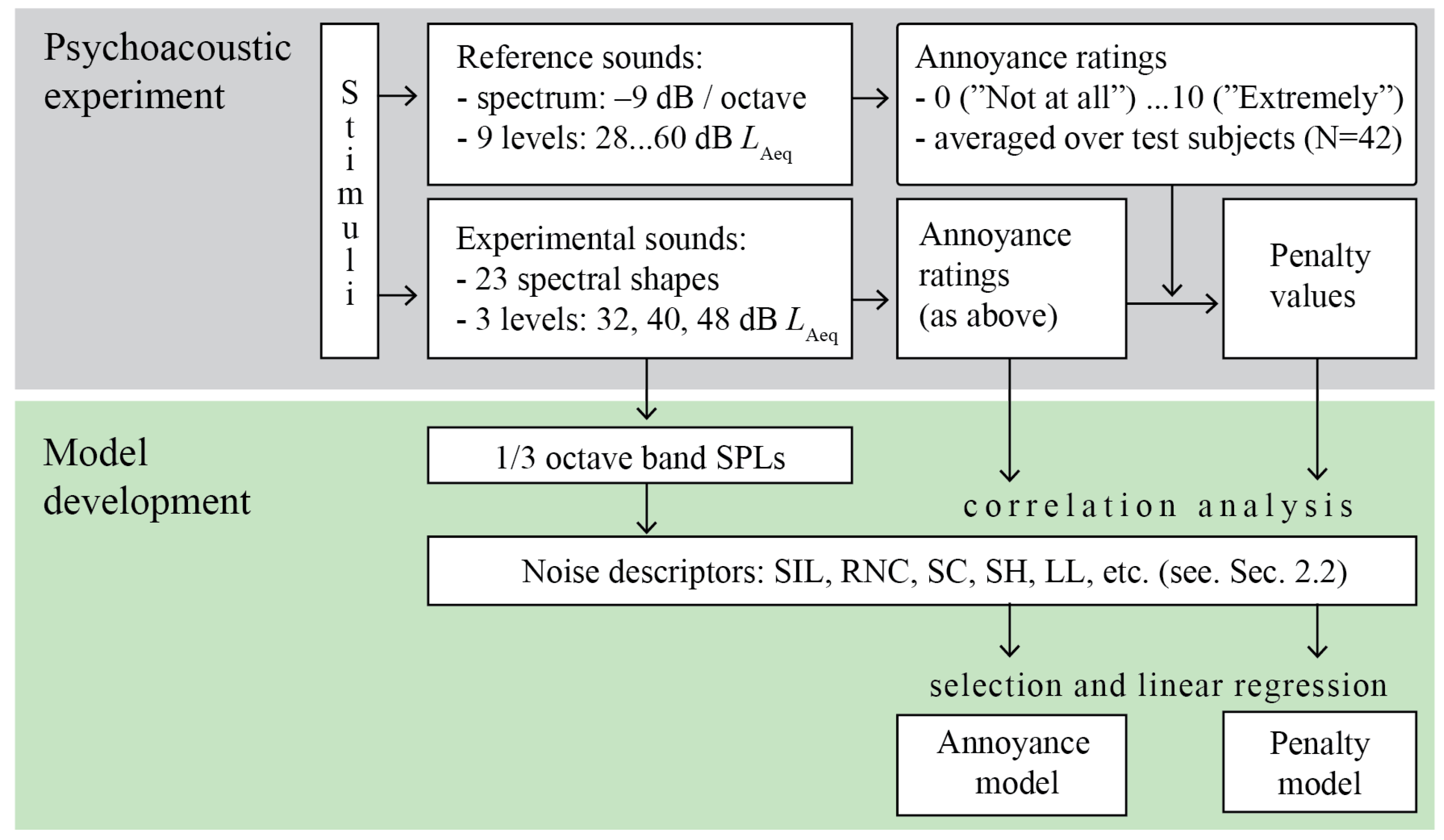
Figure 1 illustrates the workflow adopted in this study. Subjective data used for developing the models comprised annoyance ratings and penalty values for 69 steady-state noise sounds (23 spectral shapes at three L Aeq levels). One-third octave band SPLs were used to compute a range of single-number noise descriptors (presented in Section 2.2). Correlation analyses were used to identify the most relevant descriptors, and linear regression was used to model annoyance ratings and penalty. The following sections provide a more detailed description of these steps.

2.1. Psychoacoustic Experiment

Subjective data was obtained from a psychoacoustic experiment by Kuusinen et al. [5]. In the experiment, 42 people gave annoyance ratings for 23 broadband noises with distinct spectral shapes, each with three sound levels: 32, 40, and 48 dB L Aeq (i.e., 69 sounds in total). In addition, the stimuli included reference sounds, with a fixed spectrum slope of −9 dB per octave, presented at nine levels (28–60 dB L Aeq ).
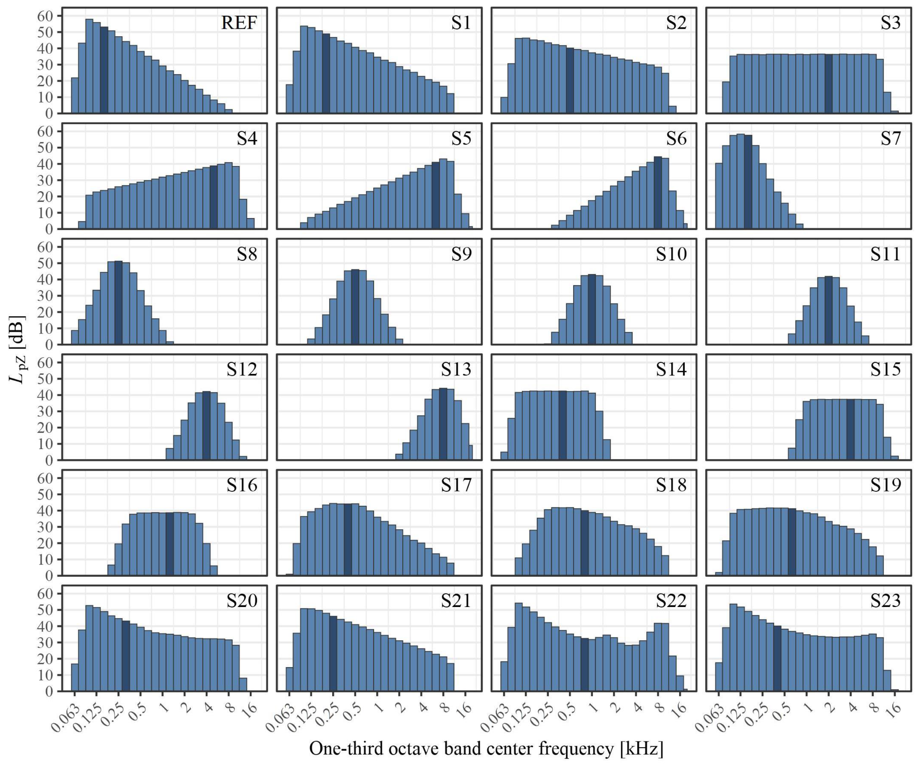
Sounds were played back with two loudspeakers (Genelec 8020D, Genelec Ltd., Iisalmi, Finland) hidden above the suspended ceiling and they could be perceived, for example, as originating from the ventilation system of the room. Sound spectra at 48 dB L Aeq are shown in Figure 2, and one-third octave SPLs are tabulated in Table S1 (Supplementary Materials). The reference spectrum is also illustrated in Figure 2. This spectrum was selected as the reference because it had been previously observed to be among the least annoying spectra [15]. Sound examples to listen to are included in the Supplementary Materials (Audio S1).
Annoyance was rated on an 11-point scale (0 = “Not at all” to 10 = “Extremely”) in response to the following question: “How much does the sound disturb, annoy, or bother you?” No contextual information was provided. Penalty ratings for the 69 spectrally modified sounds were derived by using the responses to the reference sounds (procedure illustrated in Figure S1, Supplementary Materials). Table 1 presents the annoyance ratings and penalty values averaged over the participants. These values were used for the current study. Only the data of the 69 experimental sounds is included because the penalty values are not meaningful for the reference sounds.
Preliminary observations by Kuusinen et al. [5] indicated that L Aeq significantly influenced annoyance ratings for all sounds within the 32–48 dB range. Furthermore, sounds with greater high-frequency energy relative to low-frequency energy were rated as more annoying and had larger penalty values. For instance, hissy sounds such as S6, S13, and S16 had larger k values, compared to sounds like S1 and S7, with sound energy concentrated in lower-frequency bands.
An important observation for the current study was that the annoyance ratings were observed to be level-dependent, whereas penalty values were level-independent, reflecting primarily the influence of spectral shape. This relationship is also illustrated in Figure S2 (Supplementary Material). This distinction forms the basis for analyzing associations with objective noise descriptors, which were not addressed in the preliminary analysis by Kuusinen et al. [5].

2.2. Noise Descriptors

The noise descriptors were categorized into level-dependent descriptors and (level-independent) spectral shape descriptors based on the observations in [5]. We considered level-dependent descriptors to be directly influenced by L Aeq , whereas spectral shape descriptors quantify characteristics of the spectral shape and were considered level-independent. As mentioned, distinguishing level-dependent and spectral shape indices is important in our study because the annoyance ratings were observed to be level-dependent, whereas penalty values were level-independent (see Table 1, and the illustration in Figure S2 in Supplementary Materials).

2.2.1. Level-Dependent Descriptors

The following level-dependent descriptors were considered.
L Aeq , L Zeq [dB]. These a broadband A- and Z-weighted (i.e., non-weighted) equivalent SPLs. L Aeq , L Zeq levels are equivalent to the level of a continuous steady-state noise that has the same duration as the measurement. Values were measured with a calibrated sound level meter (Nti Audio XL2).
Speech Interference Level ( S I L ) quantifies the sound level at the frequencies important for speech communication. It is calculated as the arithmetic average S P L over the 500, 1000, 2000, and 4000 Hz octave frequency bands [19,37]. Hongisto et al. [15] found S I L to be strongly correlated with the overall acoustic satisfaction of steady-state noises. They recommended S I L to be used as the primary noise index for assessing noise in office environments due to its simplicity in terms of calculation.
Noise Criterion ( N C ). Calculation of N C is based on S I L , meaning that the N C curve to compare the measured values with is selected by the S I L value. If some measured value is over the selected curve, the tangency method is used to derive the N C value. The tangency method involves superimposing measured octave band S P L values over the rating curves. The rating is determined by the curve just above (i.e., “touching”) the measured S P L values [18,19].
Preferred Noise Criterion ( P N C ). The procedure is the same as for N C , but instead of S I L , the P N C curve is selected based on preferred S I L , which is the average 500, 1000, and 2000 Hz octave bands [38].
Noise Rating ( N R ). N R rating is determined by the tangency method. Functions to derive N R curves are specified in the BS 8233 standard [39].
Balanced Noise Criterion ( N C B ). N C B curves follow the equal-loudness-level contours, so they are more closely spaced at low frequencies than at higher ones. The N C B rating was developed to be consistent with loudness perception. The S I L value is used to select the reference N C B curve to compare the measured SPLs with. Additional qualification of the rating is added if the noise contains “rumble” or “hiss” [21]. As mentioned, this additional qualification is not included in our work.
Room Criterion ( R C ). R C rating curves are parallel lines with a constant slope of −5 dB per octave. The R C value/curve is determined by the value at 1 kHz that equals the arithmetic average of measured SPLs over 500, 1000, and 2000 Hz octave bands. The R C procedure includes a separate assessment of spectral shape for rumble (‘R’), hiss (‘H’), neutral (‘N’), and tonal (‘T’) [18,20]. This additional qualification is not included in our work.
Room Noise Criterion ( R N C ). R N C curves can be considered as an “average” of N C B and R C curves. They basically follow the N C B curve shapes at low frequencies between 16 to 250 Hz, but at the higher frequencies from 250 to 8000 Hz they follow the R C curve shapes. R N C was developed to better consider the possible low-frequency effects of poorly designed HVAC systems (e.g., surging, turbulence, and rattling) than the N C B rating scheme, but also not to be as restrictive as the R C curves when the low frequencies are not problematic. The R N C rating value is determined by the tangency method (as described for N C ) [18]. The evaluation of low-frequency effects is not included in this study.
Loudness level ( L L ) [phons]. Loudness level was calculated using the Zwicker loudness model, as specified in the ISO 532-1:2017 [26] standard. The Zwicker model is appropriate for monophonic steady-state noise signals. Loudness level was computed using the acousticLoudness function in Matlab (R2024a), with 1/3-octave band S P L values as the input. The input values are included in Table S1 (Supplementary Material).
Loudness level + sharpness ( L L S H ). We adapted the perceptual annoyance model proposed by Fastl and Zwicker [24] to comprise LL and sharpness ( S H ) only. Roughness and fluctuation strength were excluded because they are not relevant for stationary signals lacking amplitude modulations. The adapted equation was L L S H = L L × ( 1 + W ( S H ) ) , where L L is the loudness level and W ( S H ) is the contribution of sharpness: W ( S H ) = max ( 0 , S H 1.75 ) × ( 0.25 + log 10 ( L L + 10 ) ) . Calculation of S H is described in Section 2.2.2.

2.2.2. Spectral Shape Descriptors

The following spectral shape descriptors were considered.
The spectral centroid ( S C ) is an estimate of the center location of the sound energy “mass” on the frequency scale [40]. The mathematical formula of the spectral centroid, S C [Hz], is as follows:
S C = n = 1 N ( f n · x n ) / n = 1 N x n ,
where f n [Hz] represents the center frequency of one-third octave band n, x n is the unweighted S P L [dB] of the band n, and N is the number of bands.
Spectral spread ( S S ) is an estimate of the spread of sound energy around the spectral centroid [41]. Correspondingly, the mathematical formula of spectral spread, S S [Hz], is as follows: S S = ( n = 1 N ( f n S C ) 2 × x n ) / n = 1 N x n .
Both S C and S S are conventionally derived from sound signals via Fourier transformation. However, we calculated the values using one-third octave band S P L values since they are readily available in practical noise measurements.
It is important to note the practical limitations in S C calculation. Because S C is calculated as a weighted mean, even very small S P L values in the highest-frequency bands would potentially have a strong influence on the final S C value. However, the frequency components with very small SPLs, especially if they are below hearing threshold levels, have no perceptual relevance and their influence should be removed from the calculation. Therefore, S P L (i.e., x n ) values that were below hearing threshold levels of ISO 389-7 [42] were set to zero to eliminate the influence of inaudible bands. In addition, S P L values below 15 dB were also set to zero because there is always some low-level background noise, such as electric noise, present in measured S P L values, which is perceptually irrelevant when the overall sound level is 32 dB L Aeq or higher.
Sharpness ( S H ) is a measure of high-frequency content in a sound. The higher the concentration of sound energy at high frequencies, the sharper the sound. The calculation procedure of S H is like that of S C , but it is based on specific loudness level values on the Bark scale weighted according to a specific weighting scheme. Sharpness was calculated using the acousticSharpness function in Matlab (R2024a), with one-third octave S P L values as the input parameter. The default weighting scheme of DIN 45692 [43] was used. Specific details of the algorithm are omitted here for brevity. More information is given by Fastl and Zwicker [24] and Matlab (R2024a) documentation (acousticSharpness function).
L Alohi is calculated as the level difference between the low (125–500 Hz) and high (1000–8000 Hz) A-weighted octave band levels. Note that in previous studies by Veitch et al. [16] and Hongisto et al. [15], the low-frequency range for L Alohi was 16 to 500 Hz. In this study, the lowest bands (16–63 Hz) were excluded because the experimental sounds in [5] were band-passed between 100 Hz and 10 kHz.
N r a t i o and N l o w were introduced by Töpken and van de Par [36]. Both employ specific loudness levels on the Bark scale. N r a t i o is the ratio between the loudness levels at low (2–5 barks, approximately 100–500 Hz) and high (10–24 barks, approximately 1100–16,000 Hz) frequencies. N l o w is calculated as the level of the lowest (0–2 barks, approximately 20–200 Hz) frequencies normalized to the overall loudness level. According to Töpken and van de Par [36], N r a t i o should distinguish between unpleasant and pleasant (fan) noises, and N l o w aims to distinguish the “humming” fan noises from the others.
Quality Assessment Index ( Q A I ). The Quality Assessment Index is an extension of the R C rating scheme introduced in the R C Mark II method [20]. It uses the same −5 dB/octave rating curves as R C . In short, the Q A I value is derived from the differences between the measured 1/1 octave spectrum and the reference curve in the low- (16, 31.5, and 63 Hz), mid- (125, 250, and 500 Hz), and high-frequency (1000, 2000, and 4000 Hz) regions. The differences are calculated by using averages of sound energy, and Q A I is defined as the maximum difference between the low-, middle- and, high-frequency groups. Similar Q A I values may be obtained with very different spectrum shapes. In practice, Q A I is more influenced by the sound energy at the higher-frequency bands due the sloping shape of the R C rating curves.

2.3. Data Analysis

Data was analyzed with correlation analysis and linear regression. Annoyance and penalty results of each sound were averaged over the participants to focus on the overall results instead of individual differences. We used the data of the experimental sounds (N = 69) only, as penalties were derived from annoyance ratings of reference sounds, and reference sounds do not have meaningful penalty values. To maintain consistency between annoyance and penalty analyses, reference sounds were also excluded from the annoyance ratings.
Spectral centroid ( S C ) and sharpness ( S H ) values were log-transformed to linearize their relationship with annoyance and penalty, as scatterplots indicated clear non-linear patterns for these variables.
Correlation analysis involved calculating Pearson’s product-moment correlation coefficients (r) and partial correlation coefficients ( r p ) between objective noise descriptors (tabulated in Supplementary Table S2) and the mean subjective annoyance ratings and penalty values shown in Table 1. To distinguish between r and r p , we refer to the former as “simple” and the latter as “partial.” Partial correlations were computed by controlling for level effects, meaning the linear influence of sound level was removed from the simple correlation. Thus, partial correlation coefficients reflect associations attributable to spectral differences among the experimental sounds. Details of partial correlation computation follow Kim [44]. Finally, based on the correlation analysis results, the most suitable noise descriptors were selected for modeling annoyance ratings and penalty values using linear regression.
All statistical analyses and data visualizations were performed in R statistical programming language (R version 4.2.2) [45] with tidyverse [46] and ppcor [44] packages.
Generative artificial intelligence (GenAI) tools were used to assist with writing scripts for data visualization. Specifically, AI was employed to generate and optimize R code for data visualization. No GenAI tools were used to generate data or graphics beyond code assistance. All analyses, interpretations, and final visualizations were reviewed, edited and validated by the authors.

3. Results

3.1. Objective Descriptors

The descriptive statistics of the objective descriptors for the experimental sounds are summarized in Table 2. The detailed numerical values are also given Table S2 (Supplementary Materials). Note that L Aeq values may not be exactly 32, 40, or 48 dB because some variability in the measured values was accepted in the experiment.

3.2. Correlations: Level-Dependent Descriptors

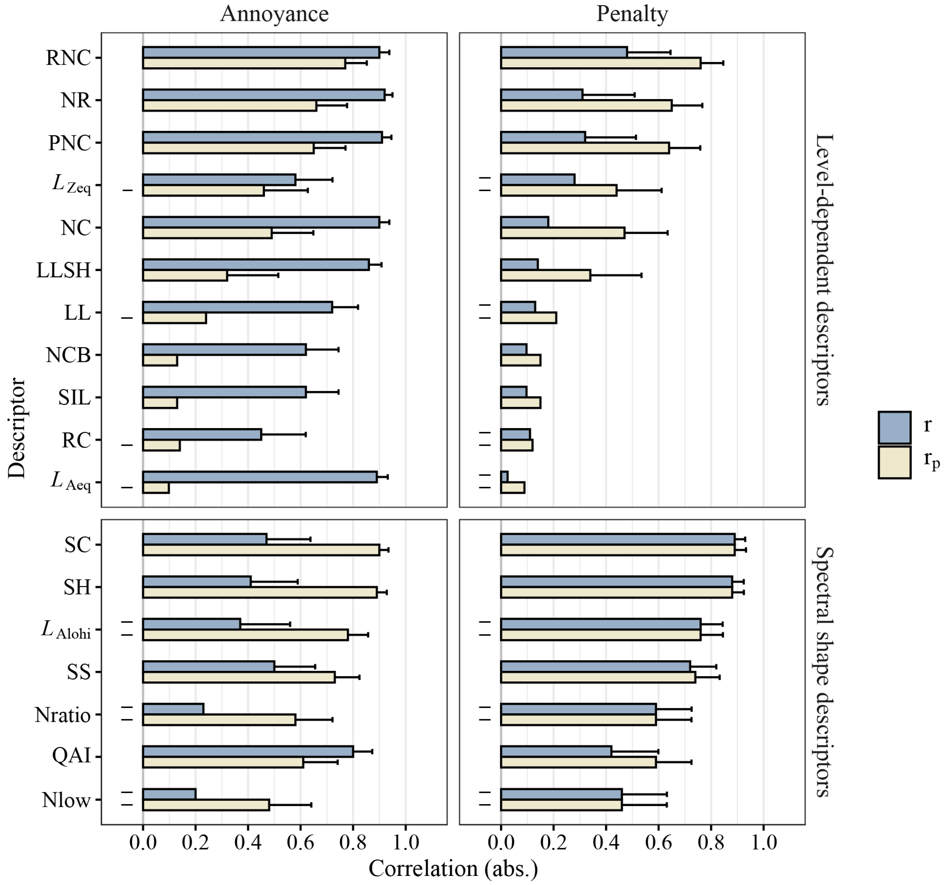
Correlation analysis results are shown in Figure 3, with numeric values in Tables S3–S6 (Supplementary Materials) and linear relationships illustrated in Figures S3–S6 (Supplementary Materials).
For level-dependent descriptors and annoyance, all simple correlations (r) were significant ( p < 0.01 ). R N C , N R , P N C , N C , L L S H , and L Aeq exhibited the highest r values (0.86–0.92), while other indices were below 0.73. Partial correlations ( r p ) were lower, with R N C showing the strongest association ( r p = 0.77).
For level-dependent descriptors and penalty, significant simple correlations were observed only for R N C (r = 0.48), P N C (r = 0.32), and N R (r = 0.31). Partial correlations were higher, with R N C again strongest ( r p = 0.77), followed by N R (0.65), P N C (0.64), N C (0.47), L Zeq (−0.44), and L L S H (0.34). Partial correlations were nearly identical whether based on annoyance ratings or penalties.

3.3. Correlations: Spectral Shape Descriptors

For spectral shape descriptors and annoyance, the highest simple correlation was observed for Q A I (r = 0.80), while others were below 0.50. Correlations were generally stronger for penalty, with all coefficients statistically significant. Particularly high values were found for S C (r = 0.89), S H (r = 0.88), and L Alohi (r = −0.76). Partial correlations for annoyance closely matched those for penalty, and differences between r and r p were minimal for most descriptors. The only exception was Q A I , where r p exceeded r ( r p = 0.59 vs. r = 0.42).

3.4. Linear Regression Models

Many level-dependent descriptors exhibited nearly equal and strong simple correlation coefficients with noise annoyance, but the partial correlations indicated R N C as the most suitable candidate for regression modeling.
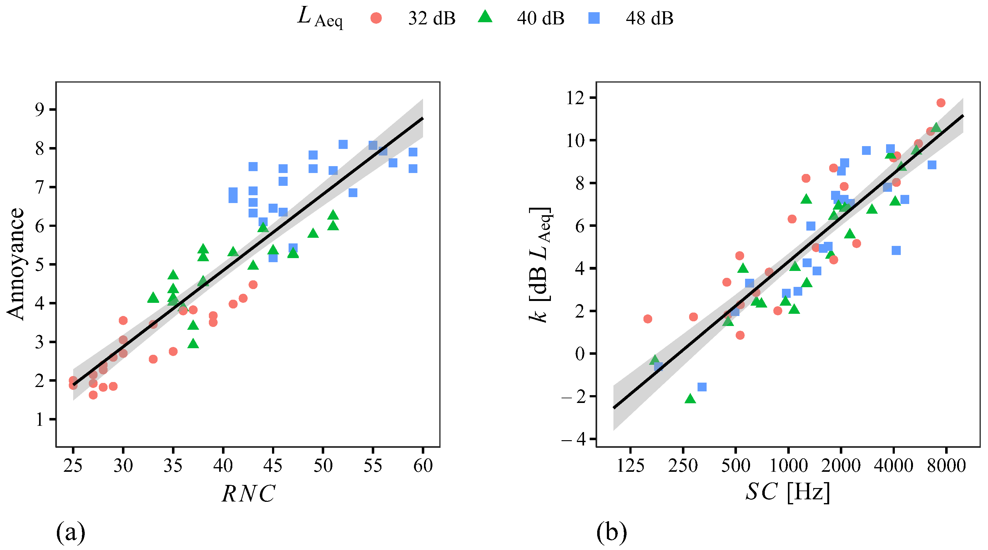
Figure 4a illustrates the linear correspondence between R N C and the annoyance ratings. The model was statistically significant (F (1,67) = 289, p < 0.001), explaining 81% of the variance ( R 2 = 0.81) with a low residual standard error ( R S E = 0.81). The estimated regression equation for annoyance, a, is as follows:
a = 0.2 × R N C 3.0
The 95% confidence intervals for the slope and the intercept for this equation were as follows: slope C I 95 % [0.17, 0.22] and intercept C I 95 % [−4.0, −2.1].
For spectral shape descriptors, S C and S H showed the strongest correlations with penalty ( S C : r = 0.89; S H : r = 0.88). Given their similarity, S C was selected for regression modeling due to its slightly higher correlation and additional advantages discussed in Section 4.2.
Figure 4b illustrates the linear relationship between S C and penalty values. The model was highly significant (F (1,67) = 252, p < 0.001), explaining 79% of the variance ( R 2 = 0.79) with a residual standard error of 1.47. The estimated regression equation for penalty, k, is as follows:
k = 6.9 × log 10 ( S C ) 16.3
The 95% confidence intervals for the slope and the intercept for this equation were as follows: slope C I 95 % [6.0, 7.7] and intercept C I 95 % [−19.0, −13.5].

4. Discussion

4.1. General

This study introduces the first objective model for determining the annoyance penalty of wideband steady-state noise (Equation (3)). Until now, the assessment of the sound spectrum has been mostly qualitative, while, for instance, tonality-based penalties are standardized ISO 1996-1:2016 [6]. Our findings highlight that the spectrum—a fundamental property of all sounds—should be assessed prior to tonality, impulsiveness, or other features that increase annoyance.
Although models for both annoyance and annoyance penalty are presented, the annoyance penalty model merits particular attention, as it offers immediate utility, for example, in environmental noise assessment and noise control strategies.

4.2. Level-Dependent Noise Descriptors and Annoyance

To begin with, the simple correlation between L Aeq and annoyance was very high (r = 0.89), while the partial correlation was near zero, as expected since L Aeq was an independent variable in the experiment. Several other descriptors ( R N C , P N C , N R , and N C ) also showed strong simple correlations, making it impossible to identify a single best descriptor based on r alone. However, partial correlations—where the effect of L Aeq was removed—indicated that R N C was the most suitable candidate, suggesting that it captures spectral influence on annoyance effectively, besides the level.
This result is unlikely due to the shape of R N C curves alone, as N C B and R C performed poorly despite the fact that they contain similar curve shapes [47]. Instead, the tangency method used to derive R N C ratings likely explains its superior performance compared to the arithmetic averaging used for N C B and R C . This interpretation aligns with Schomer and Bradley [48], who also identified R N C as a superior index compared to N C B and R C .
The R C Mark II methodology [20] includes the Quality Assessment Index ( Q A I ), which is calculated from the spectral deviations relative to the R C curve shape at a specific rating level. Q A I is intended to describe spectral shape, but our results indicate that Q A I is level-dependent, meaning that the spectral deviations vary with the sound level despite the shape remaining the same. Therefore, Q A I cannot be recommended as a spectral shape descriptor for noise annoyance assessment.
Loudness level ( L L ) did not correlate as strongly with annoyance or penalty as other descriptors. Combining L L with sharpness ( L L S H ) improved the correlation slightly but remained weaker than the best-performing descriptors. The absence of L L among the best descriptors was somewhat unexpected, as loudness is often considered a primary factor in annoyance. However, previous studies have reported similar findings for relatively soft sounds with comparable SPLs [27], where other attributes such as sharpness had greater influence. Likewise, Schäffer et al. [49] found Zwicker loudness inadequate for predicting the annoyance of noises with three different spectral shapes and different amounts of amplitude modulation. They noted that annoyance increased with low-frequency energy, which contrasts with our study, but the results are not directly comparable due to differences in frequency range (their sounds extended below 100 Hz, whereas ours were high-pass filtered at 100 Hz).
One explanation for L L ’s poor performance may be bandwidth effects: sounds with equal L Aeq but narrower bandwidths yield lower L L values [24]. In our data, some octave band bandpass-filtered sounds were rated more annoying than sounds with wider bandwidths, despite having lower L L . This discrepancy suggests that L L is not a reliable indicator of annoyance for steady-state sounds with equal L Aeq but differing spectral content. Given the broad range of spectra examined in this study, the assumption that L L predicts annoyance appears unjustified.
Ayr et al. [23] evaluated noise descriptors in office environments through occupant surveys and in situ acoustic measurements. Our results regarding noise annoyance are mostly in line with their findings. They reported correlations above 0.8 for N C , P N C , N C B , N R , R C , and R N C , but in contrast to our results, R C and N C B performed a little better than the others. Moreover, they found that L Aeq was clearly the strongest descriptor, while Zwicker’s L L also performed better than the descriptors based on the rating curves. Given that their L Aeq levels varied considerably, their finding agrees with our observation that L Aeq dominates when level variations are large (16 dB in our study). In summary, L Aeq strongly influences annoyance when level differences are substantial, whereas spectrum shape becomes more important when level variations are small.
Hongisto et al. [15] found S I L and N C B as key descriptors for assessing acoustic satisfaction with steady-state wideband noise. Our findings contradict this, as both performed poorly in our correlation analyses. This discrepancy likely stems from differences in experimental design: their study used a constant level of 42 dB L Aeq , whereas ours included three levels (32, 40, and 48 dB). The level effect, which was a key interest in our study, was notably lacking in [15] and its significance in our results was evident.

4.3. Model of Spectrum-Based Annoyance Penalty

The primary objective was to identify suitable descriptors for determining spectrum-based annoyance penalties for steady-state broadband sounds. S C , S H , and L Alohi emerged as the strongest candidates, each showing correlations near 0.9. Although L Alohi performed slightly weaker than S C and S H , it still outperformed S S , N r a t i o , and N l o w . Importantly, S C , S H , and L Alohi were largely independent of L Aeq , indicating their applicability across levels within the studied range (32–48 dB).
Many previous studies have demonstrated the association between annoyance and sharpness [9,10,11,12,13]. Our findings align with Schmidt et al. [32], who reported that sharpness was the most influential descriptor for annoyance in airborne wind energy systems at equal A-weighted levels. Moreover, the influence of S H has been found particularly apparent with relatively quiet sounds [27]. Since both S H and S C estimate the central frequency of sound energy, these findings likely extend to S C , although previous studies did not examine S C directly. In our study, both descriptors showed strong associations with penalty across three L Aeq levels (32–48 dB), reinforcing their importance in annoyance assessment.
L Alohi also emerged as a candidate, consistent with Veitch et al. [16], who found it suitable for assessing acoustic satisfaction with speech-masking sounds. However, L Alohi involves an arbitrary frequency division to “low-” and “high”-frequency regions, which is not self-evident, and it exhibited a slightly weaker correlation compared to S H and S C .
The spectral centroid was here computed using the measured SPLs in 1/3 octave frequency bands, excluding bands with S P L s below ISO 389-7 [42] hearing thresholds or 15 dB. Sharpness was calculated from the specific loudness values on the Bark scale, which were also derived from the 1/3 octave S P L values.
While both descriptors are similar, S C is simpler and more practical for environmental noise measurements and penalty assessment, as it avoids psychoacoustic conversions to the Bark scale, which is rarely used in noise measurement practice. Additionally, S C is expressed in Hertz, making it more intuitive. For these reasons, S C was selected for the regression model (Equation (3)) and is recommended for further development of spectrum-based penalty procedures.

4.4. Strengths and Weaknesses

This study is based on a single experiment using synthetic steady-state noises [5], which limits ecological validity. Real sounds often have many different features, such as temporal variations (intermittence, impulsiveness, and amplitude modulations), spatial variations, and tonality, which may also affect annoyance. Further research using real-world recordings is needed to validate the penalty model (Equation (2)) and to examine the combined effects of different features on annoyance and penalty. Current knowledge is insufficient in evaluating, for instance, how the annoyance penalty should be determined if the sound not only is “hissy” (highly annoying spectrum) but also contains prominent tones.
The model of Equation (2) can be directly applied in practical sound level measurements to determine how much penalty the sound deserves based on its spectrum. A practical example of estimating penalty with proposed model is given in the Appendix A in although the sound level range was limited to 32–48 dB L Aeq , we believe that our model can be applied in a slightly broader range, from 25 to 55 dB, because the results indicated that the annoyance penalty was level-independent within 32–48 dB. It would be important to conduct further experimental research to validate our model in this broader range and also with real-world field recordings.

5. Conclusions

This study identified objective descriptors that explained well the subjective noise annoyance of spectrally different steady-state sounds and the annoyance penalty [dB] that should be added to measured L Aeq to account for the impact of spectrum shape on the subjective annoyance.
The Room Noise Criterion ( R N C ) was the best noise descriptor that could capture both the influence of overall level and the influence of spectral shape on annoyance ratings. The regression equation was as follows: a = 0.2 × R N C 3 , where annoyance ranges from 0 (“Not at all annoying”) to 10 (“Extremely annoying”).
The spectral centroid ( S C ) was the most suitable descriptor for modeling the annoyance penalty, with the equation k = 6.9 × log 10 ( S C ) 16.3 .
Both models are expected to be applicable at least within 32–48 dB L Aeq .

Supplementary Materials

The following supporting information can be downloaded at https://www.mdpi.com/article/10.3390/app16020783/s1, Audio S1: Audiofiles in .wav-format (48 kHz, 16 bit). File names correspond to Figure 1 in the main text. Signals are normalized to full scale ([1, −1]). Table S1: Unweighted 1/3-octave band SPLs for each experimental sound. Table S2: Objective descriptor values for each experimental sound. Table S3: Correlation test results for objective descriptors correlated with annoyance ratings. Table S4: Correlation test results for objective descriptors correlated with penalty. Table S5: Partial correlation test results for objective descriptors correlated with annoyance ratings. Table S6: Partial correlation test results for objective descriptors correlated with penalty. Figure S1: The determination of annoyance penalty. Figure S2: Scatterplot of annoyance ratings and penalty values per each L Aeq level. Figure S3: Scatterplots of annoyance ratings vs. values of the level-dependent descriptors. Figure S4: Scatterplots of penalty values vs. values of the level-dependent descriptors. Figure S5: Scatterplots of annoyance ratings vs. values of the spectral shape descriptors. Figure S6: Scatterplots of penalty values vs. values of the spectral shape descriptors.

Author Contributions

Conceptualization, A.K. and V.H.; methodology, A.K. and V.H.; software, A.K.; validation, A.K. and V.H.; formal analysis, A.K.; investigation, A.K.; resources, V.H.; data curation, A.K.; writing—original draft preparation, A.K.; writing—review and editing, A.K. and V.H.; visualization, A.K.; supervision, V.H.; project administration, V.H.; funding acquisition, V.H. All authors have read and agreed to the published version of the manuscript.

Funding

This research was funded by the project “NeCom (2023–2026)” conducted by Turku University of Applied Sciences. The project was 70% funded by Business Finland [Grant 3958/31/2022]. The rest was financed by Turku University of Applied Sciences, Antti-Teollisuus Ltd., Halton Marine Ltd., Lautex Ltd., Meyer Turku Ltd., Piikkio Works Ltd., Ruukki Construction Ltd., Saint-Gobain Finland Ltd., and SBA Interior Ltd. The funders were not involved in the study design, collection, analysis, interpretation of data, the writing of this article or the decision to submit it for publication.

Institutional Review Board Statement

This study was conducted in accordance with the Declaration of Helsinki and approved by the Ethics Committee of Turku University of Applied Sciences (Ääniympäristötutkimus 2023/1, 16 March 2023).

Informed Consent Statement

Informed consent was obtained from all subjects involved in the study.

Data Availability Statement

All data to reproduce this work has been included in this article and the Supplementary Materials.

Conflicts of Interest

The authors declare no conflicts of interest. The funders had no role in the design of the study; in the collection, analyses, or interpretation of data; in the writing of the manuscript; or in the decision to publish the results.

Abbreviations

The following abbreviations are used in this manuscript:
S P L Sound pressure level
L Z e q Z-weighted equivalent sound pressure level
L A e q A-weighted equivalent sound pressure level
S I L Speech interference level
N C Noise criterion
P N C Preferred noise criterion
N C B Balanced noise criterion
N R Noise rating
R N C Room noise criterion
R C Room criterion
L L Loudness level
L L S H Loudness level + sharpness
L Alohi The level difference between the low (125–500 Hz) and high (1000–8000 Hz) A-weighted octave band levels.
Q A I Quality assessment index
S H Sharpness
S C Spectral centroid
S S Spectral spread
N r a t i o Loudness ratio
N l o w Relative loudness of low frequencies
rPearson’s product moment correlation coefficient
r p Partial Pearson’s product moment correlation coefficient

Appendix A. Example of Estimating Penalty with the Proposed Model

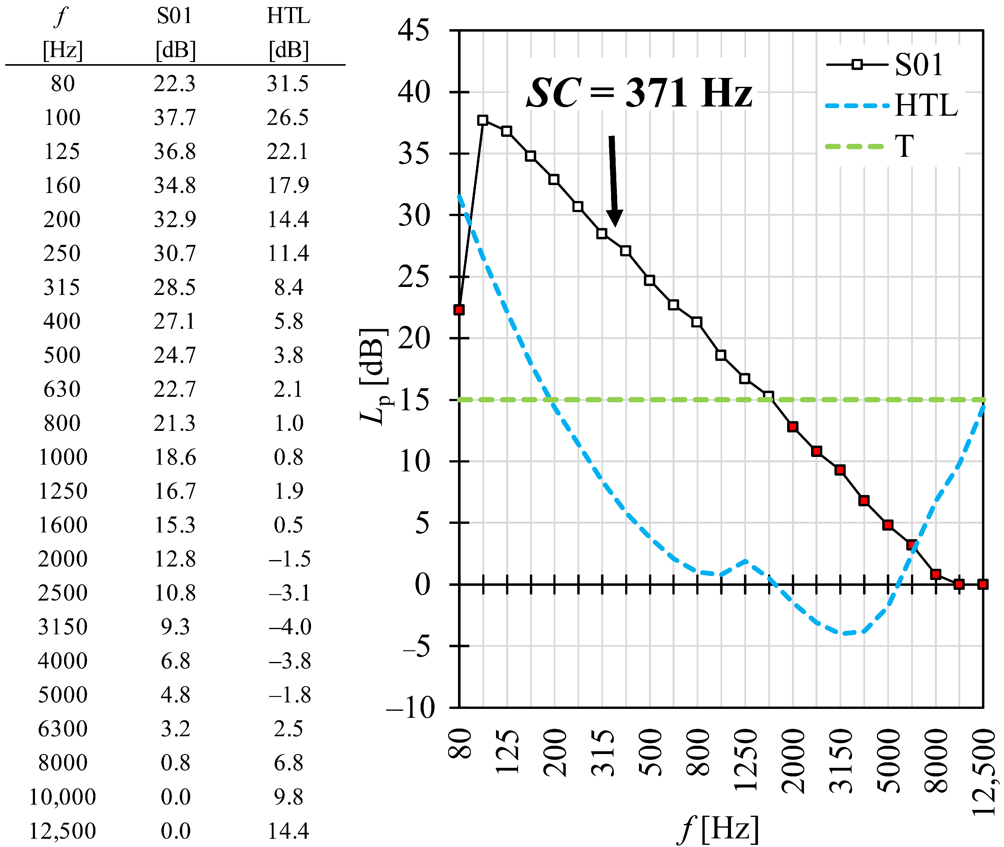
Figure A1 shows an example of the calculation procedure for sound S01 (32 dB L Aeq ). The corresponding unweighted one-third octave band sound pressure levels are presented in Table S1 (Supplementary Materials). The spectral centroid according to Equation (1) is S C = 371 Hz. Note that bands 80 Hz and 8000–12,500 Hz are not considered in the calculation of S C , since the S P L s are under the hearing threshold level of ISO 389-7. Bands 2000–6300 Hz are also ignored since the S P L s are under the threshold T (i.e., they are perceptually irrelevant).
The penalty estimate according to Equation (3) is k = 1.4 dB. Note that this value is an estimate based on the proposed model, and it is not exactly the same as the mean value reported in Table 1, which, in contrast, corresponds to the subjective annoyance ratings.
Figure A1. Example of the estimation of penalty for sound S01. H T L is the S P L of the hearing threshold according to ISO 389-7. T = 15 dB is another threshold, explained in Section 4.3. The penalty value k according to Equation (3) is 1.4 dB.
Applsci 16 00783 g0a1

References

  1. Hongisto, V. Annoyance penalties due to tonal, impulsive, and amplitude-modulated characters in sound. In Proceedings of the 14th ICBEN Congress on Noise as a Public Health Problem, Belgrade, Serbia, 18–22 June 2023; p. 178. Available online: https://www.icben.org/2023/presenting178.pdf (accessed on 4 January 2026).
  2. Oliva, D.; Hongisto, V.; Haapakangas, A. Annoyance of low-level tonal sounds—Factors affecting the penalty. Build. Environ. 2017, 123, 404–414. [Google Scholar] [CrossRef] [Scilit]
  3. Rajala, V.; Hongisto, V. Annoyance penalty of impulsive noise—The effect of impulse onset. Build. Environ. 2020, 168, 106539. [Google Scholar] [CrossRef] [Scilit]
  4. Schomer, P.D. Time of day noise adjustments or “penalties”. J. Acoust. Soc. Am. 1983, 73, 546–555. [Google Scholar] [CrossRef] [Scilit] [PubMed]
  5. Kuusinen, A.; Rantanen, E.; Hongisto, V. Annoyance penalty due to the spectrum shape of wideband noise. Build. Environ. 2024, 250, 111163. [Google Scholar] [CrossRef] [Scilit]
  6. ISO 1996-1:2016; Acoustics—Description, Measurement and Assessment of Environmental Noise—Part 1: Basic Quantities and Assessment Procedures. International Organization for Standardization: Geneva, Switzerland, 2016.
  7. ISO/PAS 1996-3:2022; Acoustics—Description, Measurement and Assessment of Environmental Noise—Part 3: Objective Method for the Measurement of Prominence of Impulsive Sounds and for Adjustment of LAeq. International Organization for Standardization: Geneva, Switzerland, 2022.
  8. Virjonen, P.; Hongisto, V.; Radun, J. Annoyance penalty of periodically amplitude-modulated wide-band sound. J. Acoust. Soc. Am. 2019, 146, 4159–4170. [Google Scholar] [CrossRef] [Scilit]
  9. Atamer, S.; Altinsoy, M.E. Sound quality of dishwashers: Annoyance perception. Appl. Acoust. 2021, 180, 108099. [Google Scholar] [CrossRef] [Scilit]
  10. Atamer, S.; Altinsoy, M.E. Vacuum Cleaner Noise Annoyance: An Investigation of Psychoacoustic Parameters, Effect of Test Methodology, and Interaction Effect between Loudness and Sharpness. Appl. Sci. 2023, 13, 6136. [Google Scholar] [CrossRef] [Scilit]
  11. Gwak, D.Y.; Han, D.; Lee, S. Sound quality factors influencing annoyance from hovering UAV. J. Sound Vib. 2020, 489, 115651. [Google Scholar] [CrossRef] [Scilit]
  12. Jeon, J.Y.; You, J.; Jeong, C.I.; Kim, S.Y.; Jho, M.J. Varying the spectral envelope of air-conditioning sounds to enhance indoor acoustic comfort. Build. Environ. 2011, 46, 739–746. [Google Scholar] [CrossRef] [Scilit]
  13. Soeta, Y.; Shimokura, R. Sound quality evaluation of air-conditioner noise based on factors of the autocorrelation function. Appl. Acoust. 2017, 124, 11–19. [Google Scholar] [CrossRef] [Scilit]
  14. Catak, N.O.; Lazoglu, I. A review of sound quality in consumer products: Research trends, metrics, and sectoral insights. J. Acoust. Soc. Am. 2025, 158, 3412–3439. [Google Scholar] [CrossRef] [Scilit]
  15. Hongisto, V.; Oliva, D.; Rekola, L. Subjective and objective rating of spectrally different pseudorandom noises—Implications for speech masking design. J. Acoust. Soc. Am. 2015, 137, 1344–1355. [Google Scholar] [CrossRef] [Scilit] [PubMed]
  16. Veitch, J.A.; Bradley, J.S.; Legault, L.M.; Norcross, S.; Svec, J.M. Masking Speech in Open-Plan Offices with Simulated Ventilation Noise: Noise Level and Spectral Composition Effects on Acoustic Satisfaction; Institute for Research in Construction: Natick, MA, USA, 2002. [Google Scholar] [CrossRef] [Scilit]
  17. Tocci, G.C. Room noise criteria—The state of the art in the year 2000. Noise News Int. 2000, 8, 106–119. [Google Scholar] [CrossRef] [Scilit]
  18. ANSI/ASA S12.2-2008; Criteria for Evaluating Room Noise. American National Standards Institute and Acoustical Society of America: Melville, NY, USA, 2008.
  19. Beranek, L.L. Revised Criteria for Noise in Buildings. Noise Control 1957, 3, 19–27. [Google Scholar] [CrossRef] [Scilit]
  20. Blazier, W.E. RC Mark II: A refined procedure for rating the noise of heating, ventilating, and air-conditioning (HVAC) systems in buildings. Noise Control Eng. J. 1997, 45, 243–250. [Google Scholar] [CrossRef] [Scilit]
  21. Beranek, L.L. Balanced noise-criterion (NCB) curves. J. Acoust. Soc. Am. 1989, 86, 650–664. [Google Scholar] [CrossRef] [Scilit]
  22. Wang, L.; Bowden, E. Finding Connections Among Indoor Noise Criteria, Human Perception, and Worker Performance. Acoust. Today 2006, 2, 33–37. [Google Scholar] [CrossRef] [Scilit]
  23. Ayr, U.; Cirillo, E.; Fato, I.; Martellotta, F. A new approach to assessing the performance of noise indices in buildings. Appl. Acoust. 2003, 64, 129–145. [Google Scholar] [CrossRef] [Scilit]
  24. Fastl, H.; Zwicker, E. Psychoacoustics: Facts and Models; Springer: Berlin/Heidelberg, Germany, 2007. [Google Scholar] [CrossRef] [Scilit]
  25. Fastl, H. The Psychoacoustics of Sound-Quality Evaluation. Acustica 1997, 83, 754–764. [Google Scholar]
  26. ISO 532-1:2017; Acoustics—Methods for Calculating Loudness—Part 1: Zwicker Method. International Organization for Standardization: Geneva, Switzerland, 2017.
  27. Berglund, B.; Preis, A.; Rankin, K. Relationship between loudness and annoyance for ten community sounds. Environ. Int. 1990, 16, 523–531. [Google Scholar] [CrossRef] [Scilit]
  28. Schlittenlacher, J.; Hashimoto, T.; Fastl, H.; Namba, S.; Kuwano, S.; Hatano, S. Loudness of pink noise and stationary technical sounds. In Proceedings of the 40th International Congress and Exposition on Noise Control Engineering 2011, INTER-NOISE 2011, Osaka, Japan, 4–7 September 2011; Volume 4. [Google Scholar]
  29. Skagerstrand, Å.; Köbler, S.; Stenfelt, S. Loudness and annoyance of disturbing sounds–perception by normal hearing subjects. Int. J. Audiol. 2017, 56, 775–783. [Google Scholar] [CrossRef] [Scilit] [PubMed]
  30. Novaković, T.; Curović, L.; Hočevar, M.; Prezelj, J. Impact of geometric modifications of small axial fans on psychoacoustic metrics. Appl. Acoust. 2024, 218, 109913. [Google Scholar] [CrossRef] [Scilit]
  31. Torija, A.J.; Li, Z.; Chaitanya, P. Psychoacoustic modelling of rotor noise. Appl. Acoust. 2022, 218, 109411. [Google Scholar] [CrossRef] [Scilit] [PubMed]
  32. Schmidt, H.; Yupa-Villanueva, R.M.; Ragni, D.; Merino-Martínez, R.; van Gool, P.J.R.; Schmehl, R. Exploring noise annoyance and sound quality for airborne wind energy systems: Insights from a listening experiment. Wind. Energy Sci. 2025, 10, 579–595. [Google Scholar] [CrossRef] [Scilit]
  33. Yang, C.; Pang, L.; Liang, J.; Cao, X.; Fan, Y.; Zhang, J. Experimental Investigation of Task Performance and Human Vigilance in Different Noise Environments. Appl. Sci. 2022, 12, 11376. [Google Scholar] [CrossRef] [Scilit]
  34. Key, K.F.; Payne, M.C. Effects of noise frequency on performance and annoyance for women and men. Percept. Mot. Ski. 1981, 52, 435–441. [Google Scholar] [CrossRef] [Scilit]
  35. Landström, U.; Åkerlund, E.; Kjellberg, A.; Tesarz, M. Exposure levels, tonal components, and noise annoyance in working environments. Environ. Int. 1995, 21, 265–275. [Google Scholar] [CrossRef] [Scilit]
  36. Töpken, S.; van de Par, S. Perceptual dimensions of fan noise and their relationship to indexes based on the specific loudness. Acta Acust. United Acust. 2019, 105, 195–209. [Google Scholar] [CrossRef] [Scilit]
  37. ANSI/ASA S12.65-2006 (R2020); American National Standard for Rating Noise with Respect to Speech Interference. American National Standards Institute and Acoustical Society of America: Melville, NY, USA, 2006.
  38. Beranek, L.L.; Blazier, W.E.; Figwer, J.J. Revision of Noise Criteria Curves. J. Acoust. Soc. Am. 1971, 50, 96. [Google Scholar] [CrossRef] [Scilit]
  39. BS 8233:2014; Guidance on Sound Insulation and Noise Reduction for Buildings. British Standards Institution: London, UK, 2014.
  40. Caclin, A.; McAdams, S.; Smith, B.K.; Winsberg, S. Acoustic correlates of timbre space dimensions: A confirmatory study using synthetic tones. J. Acoust. Soc. Am. 2005, 118, 471–482. [Google Scholar] [CrossRef] [Scilit]
  41. Peeters, G.; Giordano, B.L.; Susini, P.; Misdariis, N.; McAdams, S. The Timbre Toolbox: Extracting audio descriptors from musical signals. J. Acoust. Soc. Am. 2011, 130, 2902–2916. [Google Scholar] [CrossRef] [Scilit] [PubMed]
  42. ISO 389-7:2005; Acoustics—Reference Zero for the Calibration of Audiometric Equipment—Part 7: Reference Threshold of Hearing Under Free-Field and Diffuse-Field Listening Conditions. International Organization for Standardization: Geneva, Switzerland, 2005.
  43. DIN 45692:2009-08; Measurement Technique for the Simulation of the Auditory Sensation of Sharpness. Deutsches Institut für Normung e.V.: Berlin, Germany, 2009.
  44. Kim, S. ppcor: An R Package for a Fast Calculation to Semi-partial Correlation Coefficients. Commun. Stat. Appl. Methods 2015, 22, 665–674. [Google Scholar] [CrossRef] [Scilit]
  45. R Core Team. R: A Language and Environment for Statistical Computing; R Foundation for Statistical Computing: Vienna, Austria, 2024; Available online: https://www.R-project.org/ (accessed on 4 January 2026).
  46. Wickham, H.; Averick, M.; Bryan, J.; Chang, W.; McGowan, L.; François, R.; Grolemund, G.; Hayes, A.; Henry, L.; Hester, J.; et al. Welcome to the Tidyverse. J. Open Source Softw. 2019, 4, 1686. [Google Scholar] [CrossRef] [Scilit]
  47. Schomer, P.D. Proposed revisions to room noise criteria. Noise Control Eng. 2000, 48, 85–96. [Google Scholar] [CrossRef] [Scilit]
  48. Schomer, P.D.; Bradley, J.S. Test of proposed revisions to room noise criteria curves. Noise Control Eng. J. 2000, 48, 124–129. [Google Scholar] [CrossRef] [Scilit]
  49. Schäffer, B.; Pieren, R.; Schlittmeier, S.J.; Brink, M. Effects of different spectral shapes and amplitude modulation of broadband noise on annoyance reactions in a controlled listening experiment. Int. J. Environ. Res. Public Health 2018, 15, 1029. [Google Scholar] [CrossRef] [Scilit]
Figure 1. Overview of the workflow in this study, including the main aspects of the psychoacoustic experiment (stimuli and subjective data) and model development (computation of noise descriptors and data analysis methods).
Applsci 16 00783 g001
Figure 2. The unweighted SPLs, L pZ [dB], in one-third octave band center frequencies for the experimental sounds at the 48 dB L Aeq level. The band containing the spectral centroid is highlighted with a darker shade. The one-third octave band values are also tabulated in Table S1 (Supplementary Materials).
Applsci 16 00783 g002
Figure 3. Pearson’s simple correlation coefficients, r, and partial correlations, r p , between the objective descriptors and the annoyance ratings of the 69 experimental sounds. Negative correlations are denoted with a minus sign (−). Partial correlations were calculated by controlling for the level (i.e., L Aeq ). Whiskers denote the upper limit of 95% confidence intervals of the correlation coefficients, and they are drawn only for correlations that were statistically significantly different from zero (p < 0.01). The abbreviations of the descriptors are explained in Section 2.2.
Applsci 16 00783 g003
Figure 4. Scatterplots and linear correspondence between (a) the Room Noise Criterion ( R N C ) and annoyance ratings and (b) the spectral centroid ( S C ) and penalty scores. The thick black lines illustrate the linear models of Equations (2) and (3), respectively. Grey areas illustrate the 95% confidence intervals. Different colors and shapes represent the three L Aeq levels.
Applsci 16 00783 g004
Table 1. Mean annoyance ratings and the corresponding annoyance penalty values, k, for the 23 spectrally modified sounds at the three L Aeq levels, 32, 40, and 48 dB. The data is based on Kuusinen et al. [5] with the permission of the publisher.
AnnoyancePenalty, k [dB]
ID32 dB40 dB48 dB32 dB40 dB48 dB
S11.94.16.71.82.34.3
S22.44.77.53.84.67.4
S32.85.07.45.25.67.0
S43.55.28.18.06.79.5
S54.05.87.69.88.77.8
S64.16.07.510.49.57.2
S71.83.45.41.6−0.4−0.6
S81.92.95.21.7−2.2−1.6
S92.64.56.44.63.93.3
S103.04.66.36.34.02.9
S113.55.37.57.86.97.2
S123.85.36.89.37.14.8
S134.56.27.911.810.58.8
S142.33.96.13.31.52.0
S153.55.47.28.27.26.0
S163.85.98.19.29.39.6
S171.64.16.30.92.42.8
S181.94.36.92.03.35.0
S192.14.06.62.92.03.9
S202.75.27.55.06.47.2
S212.04.16.92.32.44.9
S222.55.37.84.46.98.6
S233.75.37.98.76.88.9
Table 2. Descriptive statistics of the objective descriptors for the sounds in Table 1. Abbreviations: “M” = mean; “SD” = standard deviation; “MD” = median; “Min” = minimum; “Max” = Maximum; “Q1” = first quartile, i.e., the 25th percentile; “Q3”, third quartile, i.e., the 75th quartile.
DescriptorMSDMDMinMaxQ1Q3
L Zeq [dB]46.66.345.737.363.442.050.2
L Aeq [dB]40.46.640.432.048.732.548.2
S I L [dB]26.88.525.09.042.021.033.0
N C 37.87.737.024.052.032.044.0
P N C 40.47.940.025.056.036.046.0
N C B 27.88.526.010.043.022.034.0
N R 40.07.740.027.055.035.046.0
R N C 40.38.741.025.059.035.046.0
R C 27.510.027.07.044.022.035.0
L L [phon]53.29.454.032.069.046.060.0
L L S H 3.32.03.20.87.51.64.1
L Alohi [dB]−7.617.6−1.7−41.832.3−23.53.1
Q A I [dB]28.88.129.214.350.922.333.9
S H [acum]1.81.31.40.35.90.92.6
S C [Hz]21171805168815774517012794
S S [Hz]1560105217734930205342637
N r a t i o 1.53.50.60.019.00.11.1
N l o w 0.10.10.00.00.40.00.1
Disclaimer/Publisher’s Note: The statements, opinions and data contained in all publications are solely those of the individual author(s) and contributor(s) and not of MDPI and/or the editor(s). MDPI and/or the editor(s) disclaim responsibility for any injury to people or property resulting from any ideas, methods, instructions or products referred to in the content.