1. Introduction
Electroencephalography (EEG) is commonly used in clinical diagnostics to detect epilepsy, brain tumors, and sleep disorders, among other neurological conditions [
1,
2]. Diagnoses are made by identifying evolving or stationary patterns across different brain regions. EEG signals also convey information about a subject’s mental state, as patterns in specific spectral regions are known to correspond to distinct cognitive conditions. For example, low-frequency activity is associated with relaxed or drowsy states, whereas higher-frequency activity reflects concentration and cognitive engagement [
3,
4]. More recently, machine learning (ML) expanded EEG analysis beyond manual inspection, enabling the automatic extraction and classification of complex patterns from raw signals. These developments allow for continuous patient monitoring and brain–computer interface (BCI) applications. Representative application areas include emotion recognition [
5,
6], mental workload assessment [
7], sleep-stage classification [
8], motor imagery decoding [
9], and, more recently, inner-speech recognition [
10].
The application of machine learning models to EEG analysis presents challenges that begin with how the data are represented [
11]. Some studies use the raw time series directly as input to convolutional neural networks (CNNs) to extract spatial patterns [
12]. However, handcrafted features are often derived from the raw signals, such as band power, statistical metrics, and more recent approaches have incorporated Riemannian geometry to model the covariance structure of multichannel data [
13]. The choice of data representation depends on the intended application and strongly impact model performance. However, since it is rarely known in advance which features are most informative, feature extraction often produces redundant, irrelevant, or noisy variables, which can significantly reduce classification performance [
14,
15].
Overfitting is another constant problem in EEG classification, as small variations in electrode placement, sensor quality, or environmental noise can lead to substantial changes in the recorded signals [
16]. More critically, individual subjects often present different patterns, causing models trained on one participant to generalize poorly to others. This cross-subject variability results in a drop in classification performance when applied to unseen individuals, complicating the deployment of EEG-based machine learning systems in plug-and-play scenarios.
Performance degradation in ML is often attributed to overly complex models that, instead of learning meaningful patterns, memorize the training data by fitting it too closely. This allows the model to perform well on the training set but poorly on unseen data. However, in cross-subject problems, the issue can arise even before model training. Although the model may learn effectively from the training data, the behavior of the testing data can differ depending on how features are defined and processed. Certain features may capture properties that vary across subjects, while others remain invariant, which can affect generalization. To address this issue, this work presents an extensive evaluation of how EEG preprocessing settings, such as window length, overlap, and feature construction, affect the performance and generalization of mental state classification models. Motivated by the problems of cross-subject generalization, we introduce a new perspective on feature selection (FS) grounded in correlation geometry. Rather than operating on the feature space, the proposed method represents EEG data through its correlation structure, which captures relationships among features. Correlation matrices are constructed across subjects and mental states, and features are analyzed based on how their associated patterns vary across these groups. The objective is to identify features that amplify differences between mental states while presenting consistent behavior across subjects, where each subject is treated as a different domain.
Most existing EEG-based mental state classification studies focus on either handcrafted feature extraction, deep learning representations, or data augmentation strategies to improve performance [
2,
4,
17]. In contrast, this work addresses the problem of cross-subject generalization directly at the feature selection level by explicitly modeling feature correlations and their stability across subjects. This distinction is particularly relevant for practical BCI systems, where subject-specific calibration or synthetic data generation may be infeasible.
A more subtle contribution of this work is the distinction between local and global generalization. Local generalization focuses on data from a single domain and is only concerned with separating mental states. In contrast, global generalization aims to preserve class separability while ensuring invariance across subjects. By changing how distances between correlation matrices are computed and aggregated, the method allows transitioning between these two regimes.
The proposed method is systematically evaluated and compared against established feature selection and dimensionality reduction (DR) techniques in the context of EEG mental state classification. Beyond classification performance, the method provides intuitive visualizations that expose shifts in data structure across subjects and states, offering additional understanding about the sources of generalization and overfitting.
The main contributions of this work are summarized as follows:
A correlation-based feature selection framework that jointly accounts for class separability and inter-subject domain invariance.
A simple and interpretable visualization for detecting structural shifts across subjects and mental states.
Flexibility to transition between local and global generalization in EEG feature analysis.
An extensive experimental evaluation on EEG mental state classification, including comparisons with established FS and DR methods.
The paper is organized as follows.
Section 2 discusses the challenges associated with cross-subject variability in EEG-based classification.
Section 3 provides background on EEG data acquisition, preprocessing procedures, feature extraction strategies, and common FS and DR techniques used to define model inputs.
Section 4 introduces the proposed correlation-based method and presents the implementation pseudocode.
Section 5 describes the experimental setup and evaluation, detailing the datasets, preprocessing parameters, and model configurations.
Section 6 reports the experimental results across multiple scenarios, followed by a discussion of the findings. Finally,
Section 7 concludes the paper.
2. Cross-Subject Problem
Most publicly available EEG datasets are collected from a limited pool of subjects [
16] under controlled experimental conditions. Although this allows reproducibility and scientific analysis, it does not fully reflect the variability present in practical scenarios. As a result, the limited number of subjects and the low variability of recording conditions may cause models to learn subject-specific and non-transferable features, which can lead to poor performance when applied to data collected on different subjects, sensors, or experimental settings [
18].
Performance degradation on cross-subject evaluation is a well-known issue in EEG classification tasks [
19]. Methods to address this issue usually involves calibration, in which a small amount of data from a new subject is used to adapt a pretrained model [
20]. This idea aims to improve performance while using as little target subject data as possible, reducing calibration time. For example, domain-adaptive methods fine-tune the model using a limited number of samples from the target domain [
19].
From an FS perspective, few studies focus on cross-subject generalization. Outside the EEG domain, Kuo et al. [
21] proposed a multi-objective FS method based on a Non-dominated Sorting Genetic Algorithm (NSGA), which balances discriminative power and domain invariance using kernel-based measures derived from source and target distributions. Another approach, introduced by [
22], does not directly select features but instead uses labeled target-domain data to identify the most suitable training subjects for a given target subject. However, both approaches still assume access to target-domain data.
Despite these advances, cross-subject generalization in EEG remains unresolved. Although these methods do not fully solve the problem, feature selection approaches that promote domain invariance while preserving class separability remain promising. In particular, methods that use interpretable features without relying on target-domain calibration are attractive for cross-subject generalization.
3. Background
This section outlines an end-to-end pipeline for EEG classification tasks, covering the stages from data acquisition to preparing model inputs. The focus is on data handling, preprocessing, and feature engineering steps that are specific to EEG analysis, while the details of the ML models themselves are omitted, as their concepts are consistent with those used in other application domains.
3.1. EEG Data Collection
EEG is a noninvasive technique with high temporal resolution [
23] that records the brain’s electrical activity through electrodes placed on the scalp. According to the international 10–20 system [
24,
25], each electrode is labeled using a letter corresponding to a specific cortical region and a numerical index denoting its relative position. Although this spatial configuration is standardized, the number and placement of electrodes may vary across studies depending on the research objectives and equipment used. The recorded signals form multichannel time series, capturing the temporal dynamics of neural oscillations across brain regions, which are often divided into frequency bands (delta, theta, alpha, beta, and gamma) [
5,
26]. Several commercial headsets have been developed to enable low-cost, portable data acquisition [
27]. Devices such as Muse Headband [
28], Biosemi Active Two, or Emotiv EPOC are adopted in educational and affective studies [
29].
EEG datasets are usually collected from a group of subjects participating in controlled experimental studies. Each experiment is divided into trials and sessions, where participants perform tasks or respond to predefined cues designed to induce emotional states. Before each trial, participants receive detailed instructions guiding the task execution. Sessions are generally kept short to minimize mental fatigue and maintain signal quality [
10]. In some protocols, multiple sessions are conducted for the same participant using identical conditions to assess intra-subject variability and signal stability over time. Because EEG data collection is time-consuming and requires specialized equipment and supervision, the number of participants in most studies remains limited.
Many researchers rely on publicly available datasets. Initiatives such as the OpenNeuro repository facilitate data sharing [
30] to ensure consistency across studies. EEG datasets are increasingly organized according to the Brain Imaging Data Structure (BIDS) standard, which defines a common format for storing and annotating medical data [
31]. Under the BIDS convention, datasets are organized into folders by subject and session, accompanied by metadata files that describe the experimental design, recording parameters, and behavioral annotations. The repository typically distinguishes between raw data and derived data, which represent preprocessed or filtered versions with artifacts and noise removed.
3.2. Feature Extraction
Although some deep learning approaches, such as CNNs, operate directly on raw EEG time series [
12], most methods rely on feature extraction to derive compact, informative representations from the electrode signals [
32]. This approach helps mitigate overfitting and reduces computational complexity.
Feature extraction is perhaps the most consequential stage in EEG analysis, as it encodes all the information used to train the model. This study adopts an extensive collection of features originally introduced in [
33], encompassing four categories: statistical, temporal, spectral, and spatial, summarized in
Table 1.
Naturally, numerous alternative feature extraction techniques have been proposed in the EEG literature, including both handcrafted and deep features [
17]. A comprehensive implementation of all available methods lies beyond the scope of this study; however, readers seeking a broader overview of EEG feature extraction approaches are referred to [
2,
8,
34].
3.3. Feature Space Transformation
EEG data can produce a large number of features. However, high-dimensional representations often include noisy, redundant, or irrelevant variables, which may obscure meaningful patterns and reduce model performance. Features may also present variability across subjects, further complicating cross-subject generalization. Therefore, it is common to apply feature selection or dimensionality reduction techniques before training the model.
Table 2 provides a brief description of the methods evaluated in this work.
3.3.1. Feature Selection
Feature selection methods can be categorized as model-agnostic or model-dependent. Model-agnostic approaches, also known as filter methods, are independent of the learning algorithm and often rely on statistical or information-theoretic criteria, such as mutual information, correlation, or entropy, to quantify the relevance of each feature with respect to the target variable. Although computationally efficient and easy to interpret, these methods usually evaluate features individually and may fail to capture inter-feature dependencies [
35]. In contrast, model-dependent approaches evaluate subsets of features based on the performance of a specific classification model, for example, through recursive feature elimination, sequential forward selection, or embedded methods such as feature importance in random forests. Hybrid techniques combine the two paradigms, for instance, applying a lightweight filter method to reduce dimensionality before a wrapper or embedded-based fine-tuning step [
36].
A property of FS methods is that they preserve the original feature representation without applying mathematical transformations. While this maintains interpretability, it also means that information contained in discarded features is irretrievably lost before model training.
3.3.2. Dimensionality Reduction
Rather than discarding features entirely, DR techniques transform the original data into a lower-dimensional space through linear or nonlinear mappings. Classical linear approaches such as Principal Component Analysis (PCA) reorder the feature axes according to the directions of maximum variance, capturing the most significant components [
37]. Nonlinear methods, including autoencoders (AEs), learn more flexible mappings that encode the data into a latent representation capable of reconstructing the original inputs through a decoder [
38].
Unlike FS, which seeks to identify the most discriminative subset of original variables, DR aims to transform the features while maintaining their information. These methods use a new set of features; therefore, they lose the interpretable meaning of the original features.
Table 2.
Description of classical feature selection, dimensionality reduction, and the correlation-based approaches proposed in this work.
Table 2.
Description of classical feature selection, dimensionality reduction, and the correlation-based approaches proposed in this work.
| Method | Description | Reference |
|---|
| ANOVA | A statistical F-test that selects features by measuring how much its mean differs between target classes relative to its variability within classes. | [39] |
| Chi-Squared Test (Chi-2) | Ranks features by measuring statistical dependence between feature values and class labels using the chi-squared statistic. | [40] |
| Mutual Information (MI) | Estimates the mutual information between each feature and the target variable, capturing relevance and redundancy. | [41] |
| Pearson Correlation | Uses the Pearson correlation coefficient to select features and remove redundancies. | [42] |
| Correlation-Based (CFS) | Selects feature subsets by maximizing correlation with the target class while minimizing inter-feature redundancy. | [43] |
| Relief | Assigns feature weights by comparing differences between nearest neighbors of the same class (hits) and different classes (misses). | [44] |
| One Rule (OneR) | Uses simple one-rule learners to rank features based on their predictive performance. | [45] |
| LASSO | Performs embedded feature selection by imposing an penalty on regression coefficients, driving irrelevant weights to zero. | [46] |
| Genetic Algorithm (GA) | Searches for optimal feature subsets using evolutionary operators such as selection, crossover, and mutation. | [47] |
| Random Forest (RF) | Estimates feature importance based on RF models. | [48] |
| Principal Component Analysis (PCA) | Linear projection that maximizes data variance along orthogonal components. | [37] |
| Kernel PCA (kPCA) | Nonlinear extension of PCA using kernel functions to capture complex feature patterns. | [49] |
| Locally Linear Embedding (LLE) | Nonlinear dimensionality reduction method that computes a low-dimensional, neighborhood-preserving embedding of high-dimensional data. | [50] |
| Autoencoder (AE) | A neural network that encodes data into a low-dimensional latent space and reconstructs it through a decoder. | [38] |
| C-DIFS | Selects features presenting minimal dispersion of correlation vectors across subjects, ensuring domain invariance. | - |
| C-SSFS | Emphasizes features whose correlation patterns differ between mental states. | - |
| C-HDSFS(M/W/B) | Balances inter-subject invariance and state discriminability using Euclidean Mean/Wasserstein/Bhattacharyya distance. | - |
4. Correlation-Based Feature Selection
This section describes the correlation-based feature selection methodology designed to identify features that generalize across subjects while remaining discriminative of mental states. Rather than operating in the feature space, the method uses a correlation representation that captures relational behavior. This representation measures feature relevance in terms of structural consistency and separation, rather than information-based or model-dependent analysis.
The method is composed of three core components:
A correlation-based feature representation, which can be constructed using different grouping assumptions (domain, class, or joint domain-class);
A distance measure used to quantify feature stability or discriminability; and
An optimization strategy that selects features based on these distances.
By decoupling the representation, distance measure, and optimization procedure, the proposed methodology provides a flexible and extensible mechanism for feature selection. Different generalization objectives can be addressed by specifying how correlation matrices are computed and how distances between feature behaviors are measured. Each component of the methodology is described in detail before presenting specific instantiations tailored to different generalization settings.
4.1. Feature Representation, Comparison, and Selection
Let denote the feature matrix, where n is the number of samples and d the number of features. The proposed methodology evaluates feature relevance through their structural relationships. These relationships are captured using correlation matrices, which provide a compact description of inter-feature dependencies and form the basis for representation, comparison, and selection.
Given a set of samples
X, a covariance matrix is computed as:
The corresponding correlation matrix
is obtained by normalizing each covariance coefficient:
Each feature
is represented by its correlation vector
which encodes how feature
f co-varies with all other features in the representation.
Depending on how samples are grouped prior to correlation estimation, different aspects of feature behavior can be emphasized. Correlation matrices may be computed using samples belonging to the same domain (subject-wise), the same class (state-wise), or jointly across domains and classes. Let denote the correlation matrix computed for a group g, where g may correspond to a domain, a class, or a domain–class pair. The associated correlation vectors provide group-specific characterizations of feature behavior. This group idea will be clearer in a further section when the method is implemented.
The feature score is quantified by comparing correlation vectors across groups using a distance function:
where
denotes the set of groups under consideration and
is a distance measure defined over vectors or distributions of correlation vectors.
This formulation evaluates feature importance through group-dependent relational behavior. The interpretation of the distance depends explicitly on the grouping criterion used to construct the feature groups. When correlation matrices are grouped by domain, small values of indicate that the feature has stable behavior across domains, thereby supporting domain invariance. Conversely, when grouping is performed by class (state), large values of indicate that the feature captures distinct relational structures between classes, promoting class separability.
Given a relevance score
for each feature, FS is formulated as an iterative pruning process. Let
denote the initial feature set. At iteration
t, correlation matrices
are computed using only the features in
, and relevance scores
are evaluated. The least informative feature according to the selected criterion is removed,
and the process is repeated until
, where
K is the desired number of selected features.
4.2. Method Instantiations
The proposed methodology can be instantiated in different ways depending on (i) how samples are grouped for correlation estimation and (ii) which distance measure is used to compare feature correlation vectors. By specifying these two elements, the method can be tailored for different generalization objectives, such as domain invariance, class separability, or both.
Table 3 summarizes the three instantiations considered in this work, highlighting their grouping strategy, distance measure, and objective.
4.2.1. C-DIFS: Correlation Domain-Invariant Feature Selection
The C-DIFS method is designed to identify domain-invariant features. The idea is that features showing consistent inter-feature relationships across domains are more likely to generalize to unseen subjects.
Let
denote the set of domains (subjects). For each domain
, a correlation matrix
is computed using samples belonging exclusively to that domain. Each feature
is then represented by its domain correlation vector
, which encodes how feature
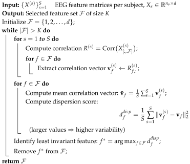
f relates to all other features within the same domain. To quantify domain invariance, C-DIFS measures the variability of these correlation vectors across domains. For each feature
f, a dispersion score is defined as
This score measures how consistently a feature’s relational structure is preserved across domains. Features with smaller dispersion values exhibit more stable correlation behavior and are therefore considered more domain-invariant.
Feature selection is performed using the pruning strategy described previously. Starting from the full feature set, features with the largest dispersion scores are iteratively removed, and correlation matrices are recomputed using only the remaining features, ensuring that feature interactions are dynamically updated during pruning. The complete C-DIFS procedure is summarized in Algorithm 1. Since it does not rely on class label information, C-DIFS can be applied in unsupervised settings.
| Algorithm 1: Correlation Domain-Invariant Feature Selection (C-DIFS) |
 |
4.2.2. C-SSFS: Correlation State-Separability Feature Selection
The C-SSFS method focuses on identifying features with discriminative relational behavior across mental states. Unlike C-DIFS, which emphasizes domain invariance, this instantiation targets class separability.
Let
denote the set of mental states. For each class
, a correlation matrix
is computed by pooling samples belonging to that class across all domains. Each feature
is then represented by its class correlation vector
, which captures how feature
f relates to all other features under mental state
c. Feature relevance is quantified by measuring the separation between correlation vectors associated with different mental states. In the binary classification setting considered in this work, a state separability score is defined as
where larger values indicate greater differences in relational behavior across states. Features with large state separability scores are therefore considered more discriminative. The complete C-SSFS procedure is summarized in Algorithm 2.
| Algorithm 2: Correlation State-Separability Feature Selection (C-SSFS) |
 |
4.2.3. C-HDSFS: Correlation Hybrid Domain–State Feature Selection
The C-HDSFS method jointly accounts for domain variability and class discrimination, targeting global generalization across subjects. This instantiation integrates the domain invariance and state separability by modeling feature behavior across both subjects and mental states.
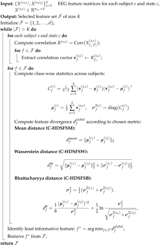
Let denote the set of domains (subjects) and the set of mental states. For each domain–class pair , a correlation matrix is computed using samples belonging to domain s and class c. Each feature is represented by its domain–class correlation vector , which characterizes the relational behavior of feature f under a specific subject and mental state. The distances can be computed using different measures, such as:
Mean Distance. A first comparison is obtained by evaluating differences in average relational behavior across subjects. For each class
c, the mean correlation vector is computed as
The global relevance of feature
f is then quantified by the Euclidean distance between class-wise means,
This measure compares the correlation vectors across subjects by treating each subject as an independent contribution to the mean correlation vector, while ignoring variance between domains.
Wasserstein Distance. To incorporate variance across domains, the distributions of correlation vectors are approximated as multivariate Gaussian distributions,
where the empirical covariance is given by
The Wasserstein distance between the two Gaussian distributions associated with classes
and
is computed as [
51]:
However, given the limited number of samples, estimating full covariance matrices is unreliable. To address this, the multivariate distributions are approximated as independent univariate Gaussians by retaining only the diagonal terms:
. The trace term simplifies to
, leading to the expression:
Bhattacharyya Distance. An alternative distributional measure is the Bhattacharyya distance [
52], which evaluates the overlap between two Gaussian distributions. For the general multivariate case, considering that
the Bhattacharyya distance is calculated by
As before, only the diagonal terms are retained:
with
Therefore, the Bhattacharyya distance simplifies to the compact form:
where all operations (multiplication, division, and logarithm) are applied element-wise.
The C-HDSFS procedure is summarized in Algorithm 3. By integrating domain invariance and class separability within a unified correlation-based formulation, C-HDSFS variants provide a mechanism for selecting features that focuses on cross-subject generalization.
| Algorithm 3: Correlation Hybrid Domain–State Feature Selection (C-HDSFS) |
 |
5. Experimental Setup
So far, we have discussed the components of EEG-based classification, from data acquisition and preprocessing to feature extraction and the formulation of the proposed method.
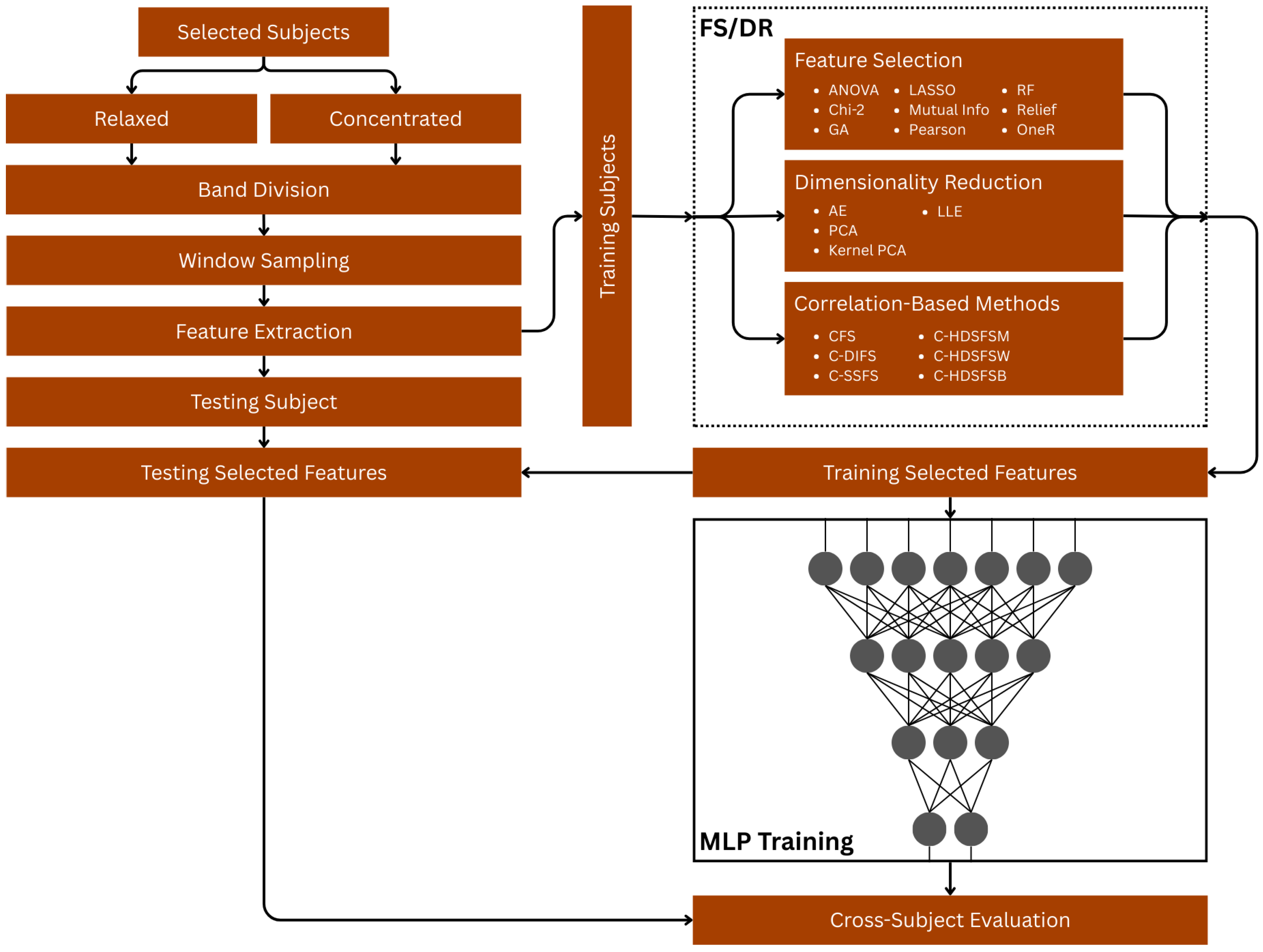
Figure 1 illustrates the complete experimental pipeline, covering all stages from EEG data collection to mental-state classification and model evaluation, which was based on [
4] work. Each block in the diagram corresponds to a specific stage, which is described in detail.
This study uses a publicly available dataset collected in [
33], aiming to capture EEG patterns associated with different mental states. Data were recorded from four participants under two controlled experimental conditions. In the concentrated condition, subjects were instructed to solve a visual puzzle task for approximately 60 s, while in the relaxed condition, they were asked to sit comfortably and perform slow, deep-breathing exercises to induce a calm state. EEG signals were acquired using the Muse headband [
28], which includes four electrodes positioned over the frontal and parietal regions, at sites TP9, AF7, AF8, and TP10, according to the international 10–20 system [
24].
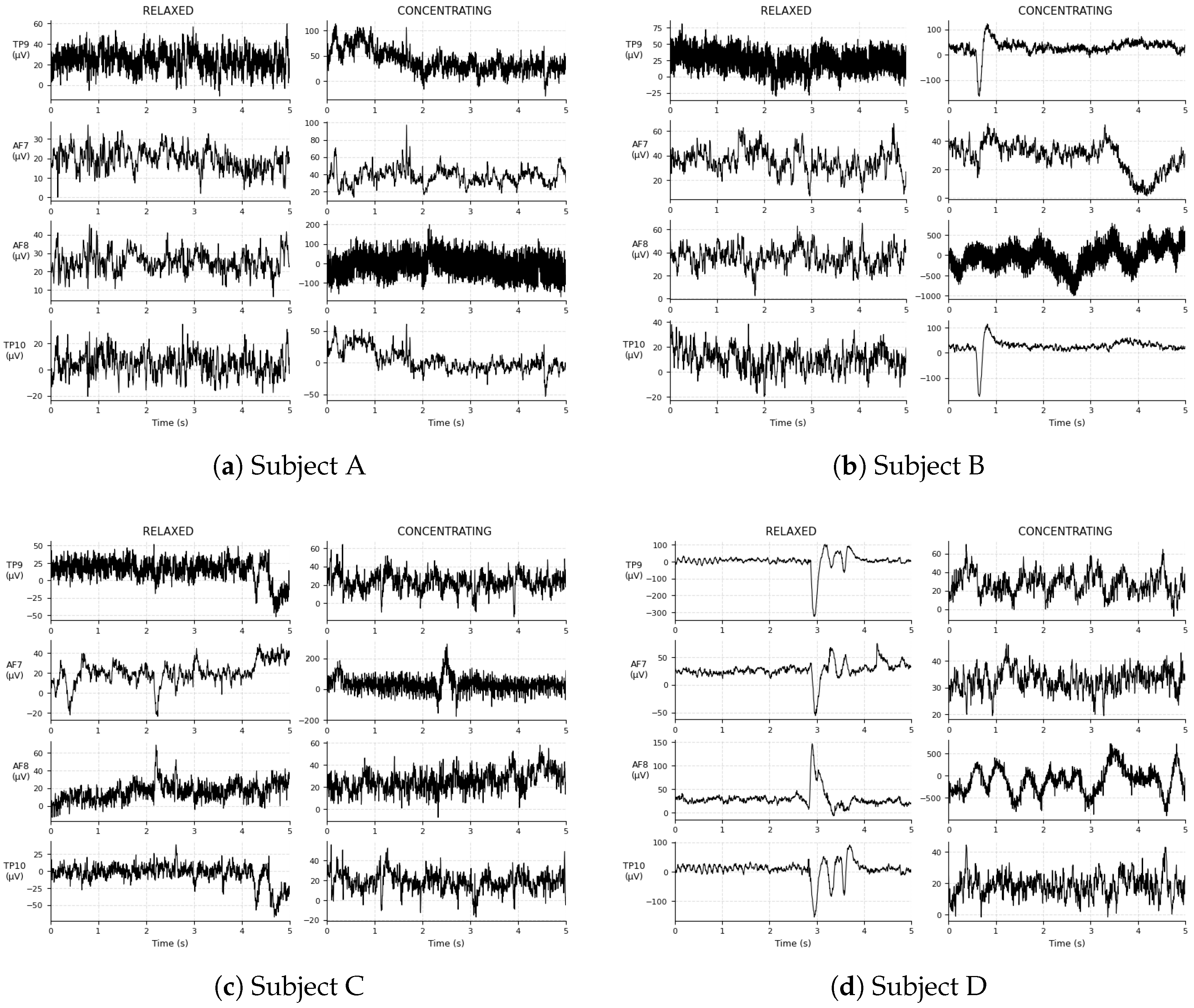
Figure 2 illustrates raw EEG recordings from each subject in both experimental conditions, showing the differences in signals between concentrated and relaxed states.
Although the analysis can be performed directly on the raw EEG signals, it is well established that specific brain patterns are associated with different frequency ranges [
53]. Therefore, the EEG signal is divided into five frequency bands: delta (0.5–3.5 Hz); theta (4–7.5 Hz); alpha (8–12 Hz); beta (12–30 Hz); and gamma (30–45 Hz), where versions of the EEG data were derived using a Butterworth filter [
54], each corresponding to one of the frequency bands above.
The raw EEG recordings are continuous multichannel time series that must be segmented into shorter, fixed-length samples for feature extraction and labeling. This segmentation process transforms the continuous signal into a collection of smaller time windows. Each window represents a specific temporal snapshot associated with a given mental-state label. The samples were created using a sliding-window approach with a fixed duration and an overlap percentage between consecutive windows. Each extracted segment is treated as an independent sample, preserving the temporal continuity of the EEG signal while increasing the number of training instances available.
Feature extraction is applied independently to each segmented EEG window, yielding a feature vector that summarizes its properties as described in
Section 3. Because the extraction process is repeated for each of the five frequency bands, the resulting feature dimensionality corresponds to the number of extracted features multiplied by five. Therefore, for the raw signal, there are 514 features, while 2556 features are available for the five bands.
The training and testing sets were defined following a leave-one-subject-out (LOSO) cross-validation strategy. In each iteration, data from three subjects were used to train the model, while the remaining subject was reserved exclusively for testing. This approach ensures that the model is evaluated on entirely unseen data from a different individual, thereby providing an assessment of its cross-subject generalization capability.
Then, feature selection, dimensionality reduction, and correlation-based methods are applied. Each technique produces a different set of features that are used to train and evaluate the classification model using identical conditions for comparison. It is important to note that, unlike feature selection, dimensionality reduction transforms the original variables into a new set of features in a lower-dimensional latent space, thereby sacrificing interpretability in exchange for potentially improved representational efficiency.
The classification model employed in this study is a multilayer perceptron (MLP) designed to evaluate different feature selection strategies rather than to maximize absolute performance. Given the limited dataset size, a shallow architecture was adopted. The network consists of an input layer that matches the feature dimensionality, followed by two fully connected hidden layers with 128 and 64 neurons, respectively, each utilizing the Rectified Linear Unit (ReLU) activation function. Dropout layers with a rate of 0.3 were inserted after each dense layer to avoid overfitting, and the output layer uses softmax to produce class probabilities. The model was trained for 50 epochs with a batch size of 64 using the Adam optimizer (learning rate = 0.001), categorical cross-entropy loss function, and accuracy as the evaluation metric. Input features were standardized within each cross-validation fold using statistics computed from the training data. No random seed was fixed to allow variability in initialization across different configuration runs. This lightweight architecture provides a benchmark for comparing the impact of FS and DR methods under identical training conditions.
The experimental setup was designed to evaluate three aspects of model performance. First, the influence of the number of selected features on classification accuracy was examined. Second, the impact of window length and overlap percentage on performance was analyzed, showing how temporal segmentation parameters affect signal representation. Finally, the model’s ability to generalize to unseen subjects was evaluated, a key criterion for practical EEG systems where subject-specific calibration is undesirable.
6. Results
6.1. Correlation Grouping Visualization
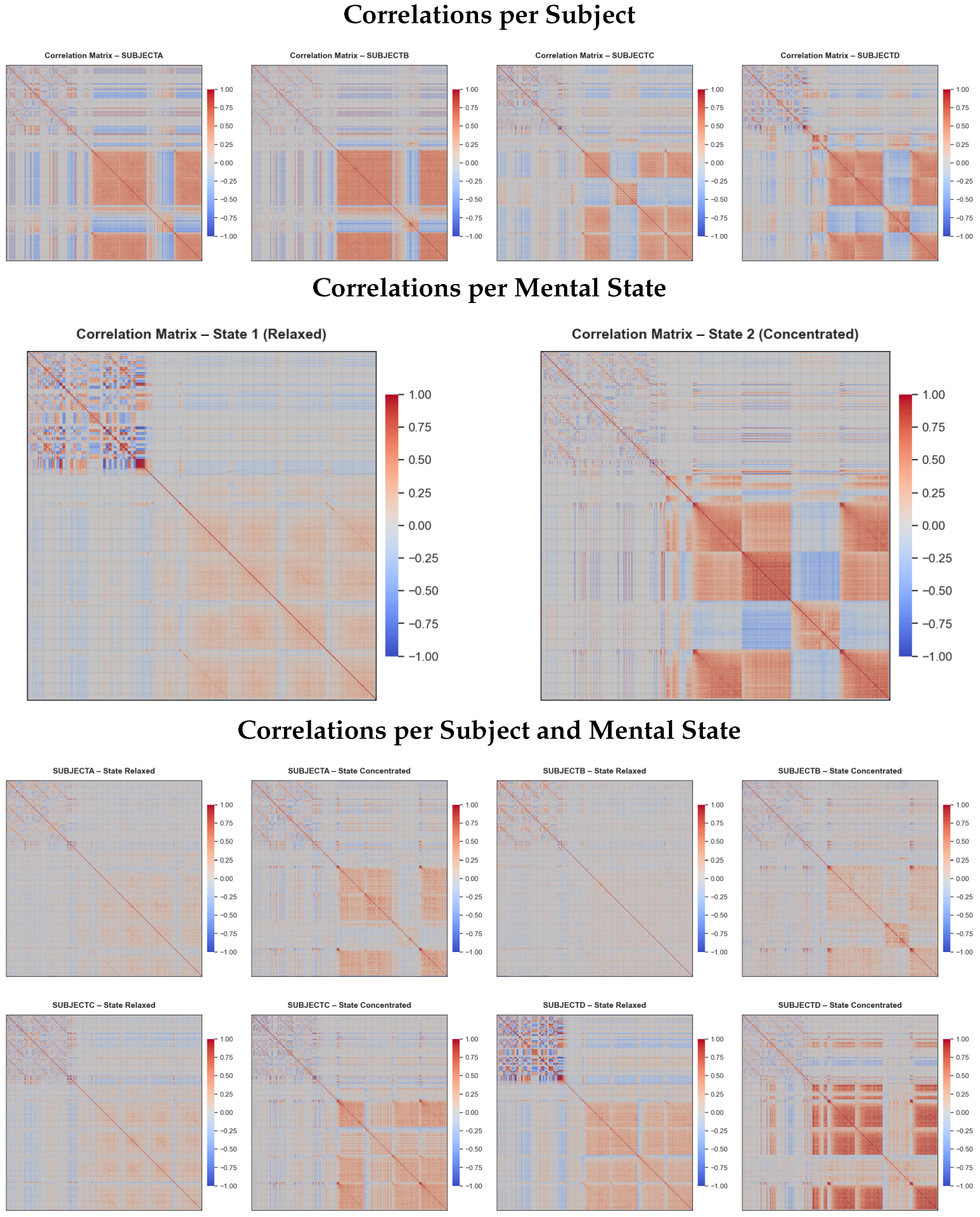
Figure 3 presents a visual analysis of the correlation structures obtained from the three method variants. The correlation matrices reveal how feature interactions vary across subjects and mental states, providing a visual understanding of feature stability and discriminability. In accordance with the LOSO protocol, the correlation matrices are computed exclusively from the training subjects, ensuring that the held-out test subject is never involved in feature selection.
The Correlation per Subject matrices were computed separately for each subject to be interpreted by method C-DIFS. Each matrix encodes the pairwise dependencies between features, representing how each feature correlates with all others. Different patterns can be observed across subjects, indicating individual variability in EEG feature relationships. In particular, Subject C exhibits a more different correlation structure compared to the others, suggesting a potential domain shift that may reduce generalization. C-SSFS uses the Correlations per Mental State matrices, where data from all training subjects are combined, and separate correlation matrices are computed for each mental state. This removes subject-specific information, allowing the analysis to focus on behavioral differences between states. In this case, features that exhibit greater structural changes between the states are expected to be more discriminative and are thus prioritized by the selection algorithm. C-HDSFS variants use the Correlation per Subject and Mental State matrices, which combine both subject and state information by computing one correlation matrix per subject and per state. From a visual inspection, Subjects A and B exhibit similar correlation structures, while Subject C retains its distinctive pattern observed earlier, and Subject D shows stronger overall magnitudes, which may indicate a larger behavioral variance between states.
6.2. Quantitative Evaluation
All experiments were conducted using a LOSO cross-validation, ensuring that each subject was excluded from training and used exclusively for testing. Two signal configurations were evaluated: (i) unfiltered EEG, using features extracted directly from the raw signals, and (ii) band-decomposed EEG, where signals were filtered into five frequency bands. Performance was evaluated across multiple dimensions, including the number of selected features, preprocessing parameters, and subject variability. Since the mental states were collected under controlled experimental conditions, the class labels were balanced and proportional to the duration of each condition. The most unbalanced subject presented 43% relaxed and 57% concentrated samples, which represents a well-distributed dataset. Although the total number of samples varies with the window size and overlap parameters, the proportion between classes remains consistent. With this balanced condition, accuracy was used as the primary evaluation metric across all experimental configurations, while the macro-F1 score was additionally reported to provide a complementary assessment of model performance.
6.2.1. Effect of Feature Dimensionality
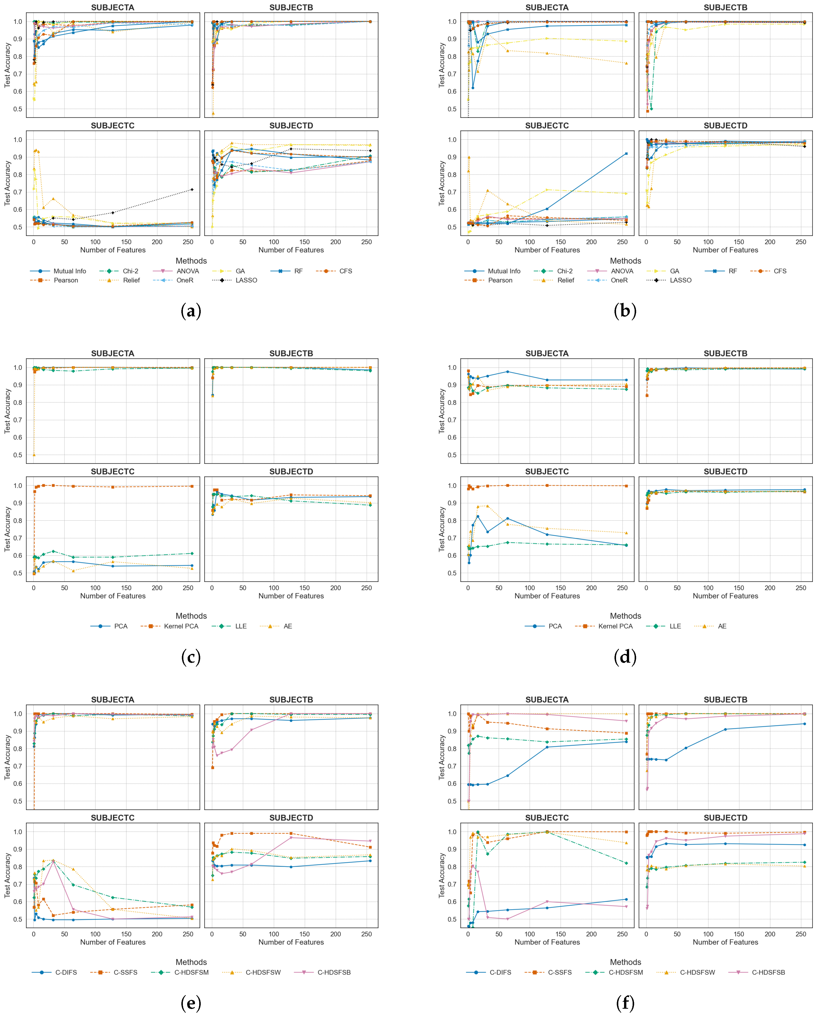
Figure 4 illustrates classification accuracy as a function of the number of selected features for both signal configurations. In this analysis, the segmentation parameters were kept fixed (window length of 1.0 s and overlap percentage of 75%), so that performance variations are attributable to changes in feature dimensionality. Results are shown separately for traditional feature selection, dimensionality reduction, and the proposed correlation-based methods.
For the unfiltered EEG, subjects A, B, and D exhibit relatively stable performance across both feature dimensionality and method choice. In contrast, Subject C presents a pronounced degradation in performance for most traditional FS and DR methods, with accuracy often converging toward chance level. This behavior highlights a strong distributional shift for this subject under cross-subject evaluation. Among the evaluated techniques, only the correlation-based methods, Relief, and Kernel PCA maintain above chance performance, especially with a lower feature number, for Subject C in this setting.
For the band-decomposed EEG, similar trends are observed. Traditional FS methods show modest improvements, with Random Forest demonstrating the strongest baseline performance as the number of features increases. Correlation-based methods demonstrate greater stability across feature numbers. Kernel PCA achieved good performance with these parameters. However, as discussed later, it exhibits high sensitivity to preprocessing conditions.
6.2.2. Effect of Preprocessing Parameters
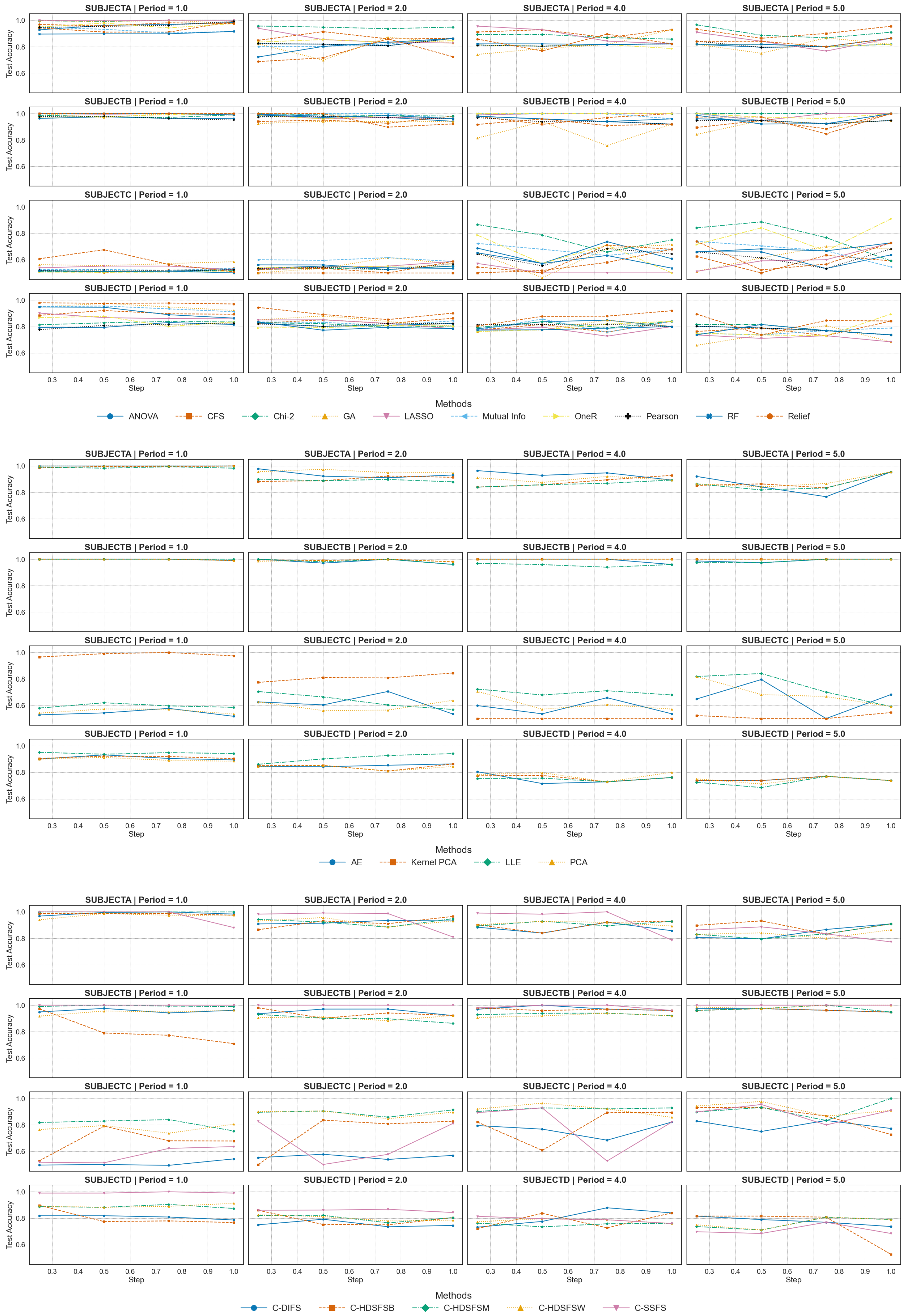
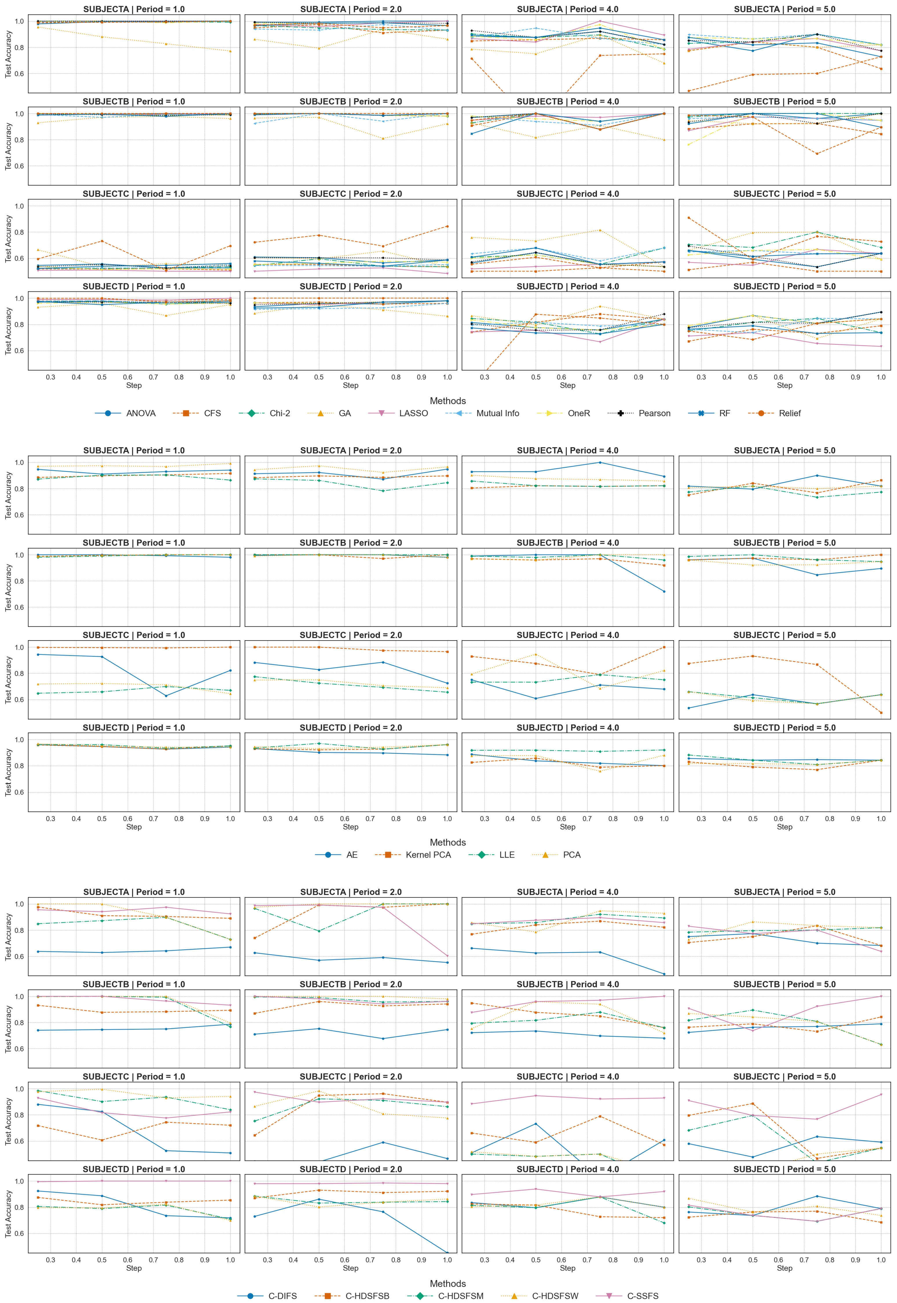
Figure 5 and
Figure 6 present results obtained by fixing the number of selected features at 32 and varying the preprocessing parameters of window length (1, 2, 4, and 5 s) and overlap percentage (75%, 50%, 25%, and 0%). Each column corresponds to a different window length, as indicated in the titles above the plots, while the x-axis represents the overlap step. The step value ranges from 0.25 (equivalent to 75% overlap) to 1.0 (equivalent to 0% overlap, a full window step). Although window overlap increases the total number of samples, it is applied uniformly across all data, ensuring that no class imbalance or bias is introduced. Furthermore, there is no temporal overlap between subjects, so the procedure fully complies with the LOSO protocol. Across both signal configurations, overlap percentage has a small impact on classification performance, while window length shows a substantial influence. For the unfiltered EEG, increasing the window length leads to a sharp performance degradation for Kernel PCA for Subject C, where accuracy approaches chance level. In contrast, the proposed correlation-based methods maintain more stable performance across the range of window sizes. For the band-decomposed EEG, Kernel PCA exhibits less performance degradation as the window length varies, whereas the C-HDSFS methods show increased instability. In contrast, C-SSFS maintains more consistent behavior across different window lengths.
6.2.3. Aggregated Performances
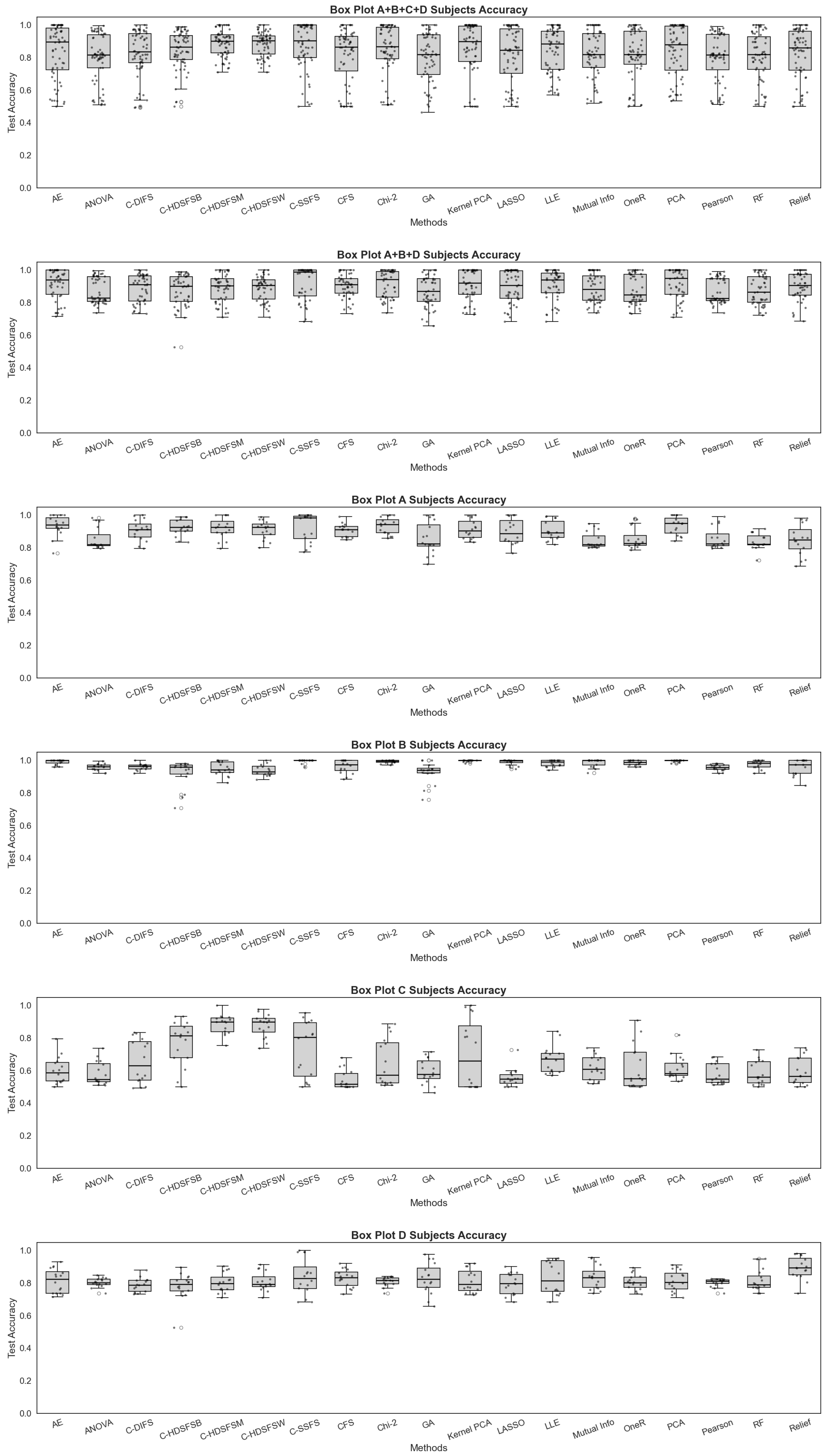
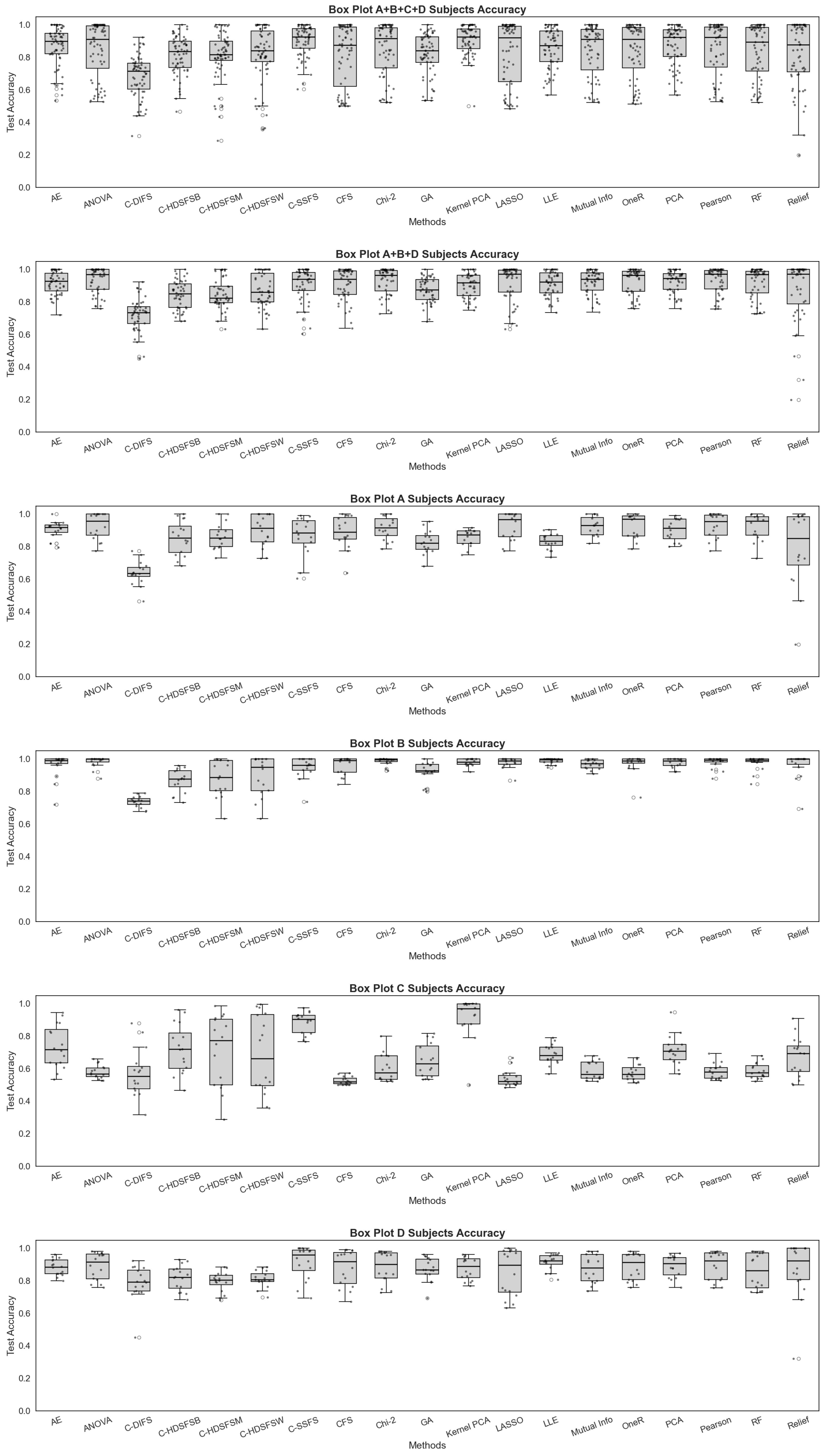
Figure 7 and
Figure 8 summarize performance across all preprocessing configurations using boxplots. Each figure presents individual subject results, the average across all subjects, and the average excluding Subject C. These plots illustrate the Subject C performance variability. For the unfiltered EEG, the C-HDSFS variants, especially those using mean and Wasserstein distances, present an improvement over all competing methods, mitigating the performance drop observed for Subject C. In contrast, for the band-decomposed EEG, Kernel PCA and C-SSFS achieve the strongest aggregated performance, while C-HDSFS variants present increased variance.
This degradation in correlation-based performance can be attributed to correlation estimation instability. Band decomposition increases the feature dimensionality by a factor of five, while the number of samples per group decreases as the window length increases. Since correlation matrices scale quadratically with feature dimensionality, insufficient sample sizes can lead to poorly conditioned correlation matrices. Among the proposed methods, C-SSFS is the least affected, as it relies on only two classes of correlation groups, whereas C-HDSFS requires multiple domain–class correlation estimates.
6.2.4. Quantitative Summary
Table 4 (unfiltered EEG) and
Table 5 (band-decomposed EEG) report the mean and standard deviation of testing accuracy across different subject combinations.
Table 6 and
Table 7 present the corresponding results using the macro-F1 metric. The overall trends observed are similar to those obtained from accuracy, both across methods and subjects; therefore, the following analysis focuses mainly on the accuracy results for simplicity. Additionally,
Table 8 summarizes the average execution time of each method applied to the band-decomposed EEG features.
The proposed methods present a higher computational cost than traditional feature selection approaches due to their iterative pruning strategy. However, feature selection is usually performed as an offline preprocessing step and does not require real-time or low-latency execution, making the observed computational complexity acceptable in practice. Furthermore, given the large number of experimental configurations evaluated in this study, a faster pruning implementation was adopted, in which ten features were removed per iteration instead of a single feature, to reduce the overall computational burden. For clarity, the correlation matrices were not recomputed at each iteration; instead, as features were pruned, the corresponding rows and columns were removed from the precomputed matrices, significantly reducing computation time while preserving equivalent results. The computational complexity of the proposed methods depends on two main factors: the calculation of the correlation matrices and the iterative pruning process. Although the number of matrices increases with the number of subjects and classes, the number of samples used in each decreases proportionally, so the overall complexity can be approximated as , where d is the number of features, n the total number of samples and p is the number of features removed per iteration. The first term corresponds to the correlation computation and the second to the iterative pruning stage.
For the unfiltered EEG, traditional feature selection presents limited cross-subject generalization for Subject C, where the best result is achieved by the Chi-2 method with an accuracy of 61.27%. Dimensionality reduction methods provide moderate improvements, although they remain sensitive to preprocessing choices; Kernel PCA, for instance, achieves 70.23% accuracy. The proposed C-HDSFSM method attains the highest score on Subject C (88.49%) while also presenting the lowest variance, indicating superior robustness to domain shifts. When results are averaged across all subjects, the C-HDSFSM and C-HDSFSW variants achieve the best performance, with accuracies of 88.84% and 88.38%, respectively. These results outperform the best DR method (85.68%) and traditional FS approaches (84.50%). When Subject C is excluded from the evaluation, C-SSFS becomes the top-performing method, reaching 91.88% accuracy, followed by PCA and the autoencoder. This behavior supports the interpretation that C-SSFS focuses on local generalization, performing best when data distributions are relatively stable, whereas the C-HDSFS variants favor global generalization and maintain performance under inter-subject variability.
For the band-decomposed EEG, Kernel PCA shows a slight improvement over C-SSFS when averaging across all subjects, achieving 90.66% accuracy compared to 90.22% for C-SSFS. However, the C-HDSFS variants experience a performance degradation. This effect is likely related to the increased number of features introduced by band decomposition combined with a limited number of samples, which can affect correlation estimation. Traditional FS methods exhibit performance comparable to the unfiltered EEG case, although with a modest improvement.
Overall, these experiments demonstrate the applicability of the proposed correlation-based feature selection methodology in scenarios both with and without significant distribution shifts between training and testing data. The results show that the proposed methods achieve competitive or superior performance compared to established feature selection and dimensionality reduction techniques, while maintaining interpretability.
These results report the mean performance obtained across the entire set of experiments conducted in this study. Among all evaluated configurations, the C-SSFS method combined with band-decomposed features, a 2s window length, and a 75% overlap achieved the best overall performance, reaching an accuracy of 98.52%.
Table 9 compares the proposed approach with representative EEG mental state classification studies using the same dataset. Although the reported accuracies are not directly comparable due to differences in the number of mental states and evaluation protocols, the table provides a reference baseline for contextualizing the expected performance on this dataset while highlighting how the present work analyzes the problem from a different perspective.
Prior studies have focused on handcrafted feature extraction, deep learning architectures, transfer learning, or synthetic data augmentation to enhance classification accuracy. However, these approaches often overlook cross-subject generalization, as they employ evaluation strategies such as k-fold or train/test splits that mix samples from all subjects in both training and testing sets [
4,
33,
55,
56]. The work in [
57] explored knowledge transfer between EMG and EEG domains and briefly examined model performance across modalities before and after transfer learning, which is related to the cross-subject problem but was not its main focus. In contrast, the proposed method explicitly targets the selection of correlated features that remain stable across subjects through correlation-based modeling. This emphasis on inter-subject invariance distinguishes the proposed approach from other methods and contributes a complementary perspective to existing EEG mental-state classification research.
Table 9.
Comparison with prior EEG mental state classification studies using the same dataset. In the Cross-Subject column, Limited denotes experiments that include multiple subjects but mix them in both training and testing, while Partial indicates a brief cross-subject test without further analysis.
Table 9.
Comparison with prior EEG mental state classification studies using the same dataset. In the Cross-Subject column, Limited denotes experiments that include multiple subjects but mix them in both training and testing, while Partial indicates a brief cross-subject test without further analysis.
| Study | Method | States | Cross-Subject | Accuracy | Year |
|---|
| Bird et al. [33] | Handcrafted + FS + ML | 3 | Limited | 87.17% | 2018 |
| Bird et al. [57] | Transfer Learning | 3 | Partial | 82.39% | 2020 |
| Bird et al. [55] | GPT-2 augmentation | 3 | Limited | 96.69% | 2021 |
| Venugopal et al. [4] | GAN augmentation | 2 | Limited | 98.45% | 2024 |
| Manoharan et al. [56] | Deep learning | 3 | Limited | 91.72% | 2024 |
| This work | Correlation-based FS | 2 | Yes | 98.52% | 2025 |
7. Conclusions
This work introduced a novel family of correlation-based feature selection methods designed to improve cross-subject EEG mental state classification. By explicitly modeling inter-feature relationships through correlation structures, the proposed framework identifies features that are both discriminative across mental states and stable across subjects, directly addressing one of the main limitations of EEG-based learning systems: inter-subject variability.
Comprehensive experiments conducted under a cross-subject evaluation protocol demonstrate that the proposed methods consistently achieve superior or competitive performance when compared to established feature selection and dimensionality reduction techniques. The results show that classification accuracy depends on preprocessing choices, such as window length and frequency band decomposition, while overlap percentage has a smaller effect. Feature dimensionality had a greater impact in the presence of pronounced data distribution shifts (Subject C). These findings highlight the importance of jointly considering signal preprocessing and feature selection. The proposed approach achieves improved generalization without relying on subject-specific calibration, deep learning architectures, or synthetic data augmentation, while maintaining feature interpretability. Overall, the findings indicate that correlation-driven feature selection provides a robust and interpretable alternative for cross-subject EEG classification tasks, particularly in scenarios characterized by strong distributional shifts.
Future work will investigate the integration of regularized and shrinkage-based correlation estimators to further improve robustness under limited data conditions, as well as alternative feature selection strategies beyond pruning to obtain more optimal feature subsets. In addition, extending the proposed framework to multi-class mental state classification, higher-density EEG systems, and other biosignals represents a promising direction for broader applicability.