DSM-Based Quantitative Comparison of Centralized and Modular Architectures of a Field-Deployed Electrohydraulic Lifting Device, Validated by Prototype Experiments

Featured Application

Modular electrohydraulic lifting units—each integrating a variable-speed pump drive, a local valve block, a reservoir and a position sensor at the cylinder—are intended for the field erection of large vertical steel storage tanks and for comparable heavy assembly operations in which six to ten lifting points must be raised in synchrony under unequal and variable load.

Abstract

Steel storage tanks are erected on site by multi-cylinder hydraulic lifting, conventionally from one power unit feeding all cylinders through a flow divider. Decentralized alternatives have not been evaluated for this task, and modularity in fluid power is rarely quantified. A ten-cylinder device was analyzed as a centralized (C1) and a modular (C3) variant with a servomotor-driven pump at each cylinder; both were decomposed into five functional modules and compared through a directed design structure matrix (DSM). External dependencies per module fell by 38.6% and mean interface complexity by 30.9%, against only 11.1% for interfaces per module: interfaces were thinned, not removed. Internal cohesion rose from 0.583 to 0.805; the total risk priority number, an ordinal expert-assigned indicator, fell from 2253 to 760. C1 was characterized from documentation and was not tested experimentally; a three-module prototype at a length scale of 0.31 was run through sixteen series: open and closed loop, both directions, four disturbance configurations. In open loop, the error left the ±2% band in every series; in closed loop, it stayed inside the band in lifting and over the last 91–92% of stroke in lowering, cutting the drift rate by one to two orders of magnitude. The structural gain corresponds to removing the hydraulic installation and the flow divider, which dominate both the open-loop drift and the failure-mode ranking; the modular device costs about 58% more.

1. Introduction

Large vertical cylindrical steel storage tanks are assembled on site from rolled shell courses. In the jacking method, the top course and the roof are erected first, and the growing shell is raised repeatedly, so that joining and inspection work stays at working height, and most of the scaffold work disappears [1]; the method remains dominant for tanks of 10–20 m diameter [2]. The shell is thin, geometrically imperfect and comparatively flexible; it is lifted at six to ten points around its circumference, and any difference between the strokes of those points enters the shell as an additional, unintended load [3]. Such assembly-induced stresses add to the design loads, whose analysis for reservoirs of this type is an active subject in itself [4].

Lifting equipment for this task is almost always hydraulic and, in commercial practice, centralized: one power unit feeds all cylinders through a multi-section flow divider and an extensive hydraulic installation of hoses and couplings.

Synchronization is therefore passive: the accuracy of the motion equals the accuracy of the divider. Catalogue split accuracy for gear dividers of this class is 2–5%, and it is further degraded in service by unequal loading of the sections, by differences in their volumetric efficiency and by the compliance and leakage of the distribution network [5,6,7]. Because the position error is the time integral of the flow difference, a deviation that is negligible at the start of a stroke can dominate at its end [8].

The hydraulic installation is also where the practical problems accumulate: one documented reference installation for a ten-cylinder device of the size considered here used 300 m of hose and 40 quick couplings. Every element adds pressure loss [9], and every detachable connection is both a potential leak and an entry point for contamination, which is reported as the cause of 70% of hydraulic failures [10,11], with the most damaging particles comparable in size to the internal clearances of the components [11,12]. Seal degradation adds a slow drift in internal leakage that is difficult to detect [13].

Safety is the second problem. The installation holds a large volume of pressurized fluid and, combined with passive synchronization, leaves loss of holding capacity and uncontrolled descent of a section as the dominant hazards [14,15,16], which lifting-operation studies show to be coupled rather than independent [17,18].

Active synchronization of hydraulic cylinders is, by contrast, a mature research field. Master–slave, equivalent and cross-coupled schemes have been reviewed repeatedly [19,20] with implementations from two-cylinder rigs to multi-cylinder electrohydraulic servo drives [21,22,23,24] reported accuracies reach 0.19–0.27 mm in a four-cylinder master–slave erection system [8] and below 0.1 mm with adaptive cross-coupling [22,23].

Recent work continues in the same direction, halving the synchronization error of a multi-cylinder heavy-machinery lift under asymmetric load by feeding the elastic deformation of the lifted structure back into the loop [25] and holding multi-cylinder synchronization within 0.5 mm under impact loading with a master–slave proportional scheme [26]. These studies refine the control algorithm on a fixed architecture; which architecture the algorithm should run on remains unexamined, remains unexamined; the present work addresses that question.

The hydraulic drive layer has been changing at the same time. In displacement (volumetric) control, a variable-speed electric motor drives a fixed-displacement pump connected directly to the cylinder; throttling losses disappear, and cylinder velocity becomes a direct function of an electrical setpoint [27,28,29]. Electro-hydrostatic actuators and direct-drive volume control built on this principle have been demonstrated from aerospace actuation to heavy-duty machinery powertrains [30,31,32,33,34,35,36,37]. The architectural consequence is that the hydraulic power path becomes short and local, while the long-shared path becomes electrical and informational. Energy consumption is not among the quantities measured in the present work; the energy argument for displacement control is taken from that literature, not re-tested here.

Whether this redistribution of functions is an improvement is a question about product architecture, not about hydraulics. The mapping between functional and physical structure, Ulrich’s definition of architecture [38], determines which changes stay local and which propagate through the product, and it has been formalized in a broad methodological literature on modular design [39,40,41,42,43]. The design structure matrix (DSM) is the standard instrument for making that structure explicit and measurable [44,45], and a large family of clustering algorithms and modularity indicators has grown around it [46,47,48,49,50], with formal roots in network modularity [51,52]. Modularity carries a price: it is routinely obtained at some penalty in performance, mass or component count [53].

A modular architecture also creates measurement points where a centralized one has none. Condition monitoring and predictive maintenance of hydraulic pumps are active research fields [54,55,56,57], and the fluid-power community has identified distributed sensing and communication as the core of its Industry 4.0 agenda [58]. Placing a pump, a valve block, and a displacement sensor at every cylinder makes each lifting point individually observable, and the sensors required for control are the same ones required for diagnosis.

Three gaps follow from this literature. First, modularity in fluid power is argued qualitatively—interchangeability, serviceability, reuse—but is rarely quantified with architecture-level indicators, so competing architectures cannot be compared before they are built. Second, experimental work on synchronization is dominated by two-cylinder laboratory rigs under symmetric load with healthy components, which is exactly the condition in which the passive centralized solution also performs acceptably; the informative comparison is made under degradation and asymmetry. Third, structural analysis and experimental verification are almost never carried out on the same object, so it remains unknown whether an architecture indicator predicts anything measurable.

This paper addresses those three gaps for one concrete device: a ten-cylinder electrohydraulic lifting system for the field erection of steel storage tanks, developed and tested in an industry-based doctoral project [59,60]. Its contributions are:

• a directed DSM formulation with four indicators and an explicit arithmetic check, applied to the centralized and modular variants of one device instead of a generic example;
• sixteen experimental series on a three-module prototype in which a reduced pump delivery and a 2:1 load asymmetry are injected deliberately, singly and in combination, in both directions of motion;
• a quantitative link between the architecture indicators, the measured synchronization behaviour and the comparative risk assessment of the same object;
• a directional diagnostic rule—effective pump delivery assessed during lifting, holding valves during lowering—derived from the measured fault signatures and requiring no additional hardware.

The remainder of the paper is organized as follows. Section 2 defines the two architectures, the DSM formulation and its indicators, the prototype rig, the experimental programme and the comparative risk assessment. Section 3 reports the structural and experimental results. Section 4 discusses the relationship between them and the limitations of the study, and Section 5 concludes.

2. Materials and Methods

2.1. Compared Architectures

The object of the comparison is a device for the synchronized lifting of large steel tank shells at ten lifting points. Both variants use identical actuators: differential cylinders with an 80 mm piston, a 50 mm rod and a 1295 mm stroke. At the nominal pressure of 9 MPa (90 bar) the piston area of 5027 mm² gives 45.2 kN per cylinder and 452 kN for the complete set. A typical field configuration has six to ten lifting points on temporary brackets around a tank of 10–20 m in diameter.

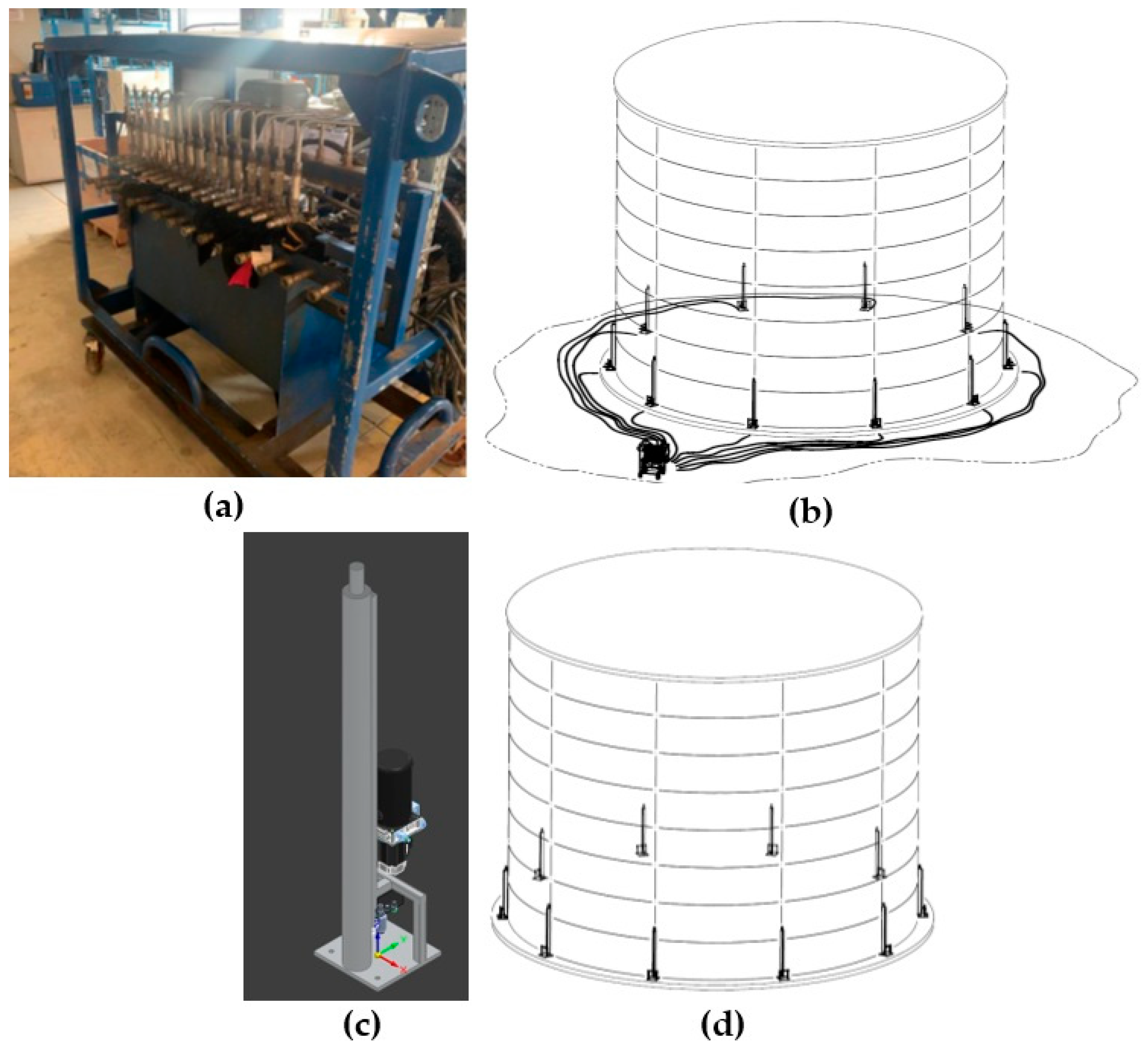
The centralized variant, denoted C1, represents current commercial practice; the unit analyzed here was supplied by a contractor specializing in tank erection: a 5.5 kW electric motor, a 14 cm³/rev gear pump running at 1500 rpm, a 100 L reservoir and a mass of approximately 270 kg without actuators. It feeds a ten-section gear flow divider, for which catalogue split accuracy in this class is 2–5%. The pump delivery of about 20 L/min gives each divider section about 2 L/min, so full extension of one cylinder (6.5 L) takes approximately 210 s. The reference installation documented for this study used 300 m of hose with 40 quick couplings.

The modular variant, denoted C3, replaces the single power unit and the divider by ten identical autonomous modules supervised by a common PLC. Each module integrates a 0.75 kW, 230 V servomotor running at up to 3000 rpm, a gear pump, a local valve block carrying the safety and holding functions, an aluminum reservoir of approximately 10 L, the cylinder and a displacement sensor, and weighs approximately 40 kg. Matching the 210 s stroke time of the centralized variant requires 1.9 L/min per cylinder, about 0.4 kW at the pump shaft against the 0.75 kW rating of the servomotor. The total fluid volume is of the same order in both variants, about 100 L, but in C3 it is divided into ten independent circuits, and the hydraulic installation of more than 300 m of hose disappears. Installed electrical power is 5.5 kW in a single unit for C1 against 7.5 kW distributed over ten units for C3, while the heaviest single item to be handled on site falls from 270 kg (without actuators) to 40 kg (with actuator).

The designations C1 and C3 are those of the underlying design study, in which an intermediate variant C2—the central power unit retained, but passive flow division replaced by proportional valves at each cylinder—was also examined; the original labels are kept here for traceability with the source documentation. C1, rather than C2, is the reference of this paper because C1 is the variant in service: it is the equipment the contractor concerned actually operates, and it is what a modular device would replace. C2 was ranked between the two in the weighted evaluation of that study, above C1 and below C3, so it is an untested intermediate rather than a discarded weak option. This limits what the comparison establishes. The results below hold against a centralized architecture with passive flow division; a comparison against individually controlled proportional sections would have to be made on the same terms before anything could be concluded about it.

Both architectures are shown in Figure 1: C1 as the power unit with the gear flow divider and as a visualization of the field installation, and C3 as a model of the autonomous module and a visualization of the corresponding installation.

2.2. Functional Decomposition and DSM Formulation

Both architectures were decomposed into five functional modules, each defined by the function it performs and not by the physical location of its parts. The number of modules was held at five in both cases, because ${IF}_{\mathrm{m}\mathrm{o}\mathrm{d}}$ and ${iw}_{\mathrm{m}\mathrm{o}\mathrm{d}}$ are per-module quantities and are comparable only at equal $N_{\mathrm{m}}$. The functional partition itself differs between the variants, and that difference is the design change under study: C1 contains a flow divider and a distribution network that C3 does not, so no partition can be held common to both, and the indicators compare architecture and partition pairs rather than alternative partitions of one fixed system, which is the decision actually faced at this stage of design. In C1, the modules are M1, generation and conditioning of hydraulic power; M2, division of flow; M3, transmission and connection; M4, actuation and load holding; and M5, measurement and supervision. In C3, the actuation function moves into the power module, and the partition becomes M1, the autonomous drive-actuation unit; M2, supervisory control; M3, electrical supply; M4, mechanical attachment; and M5, communication and diagnostics. The decomposition follows the systematic-design convention of establishing the function structure before the physical embodiment [39] and the functional modelling approach to modularization [41]. The element lists contain 21 elements for C1 and 20 for C3 and are given in

Table 1. Functional modules and their constituent elements in the centralized (C1) and modular (C3) architectures.

Module	C1—Centralized	C3—Modular
M1	Drive motor; hydraulic pump; oil tank; filtration; safety valves; cooling	Servomotor; gear pump; local hydraulic block; safety valves; cylinder; encoder/displacement sensor; local reservoir and oil circuit; module connections
M2	Gear flow divider; flow compensation; volume equalization	PLC controller; operator panel; synchronization algorithm; trajectory setting and supervision
M3	Supply lines; return lines; quick couplings; measurement ports	Drive power supply; electrical protection; emergency-stop and enable circuit
M4	Cylinders; hydraulic locks; counterbalance valves; mountings	Attachment to the structure; latch, gripper and pins
M5	Operator panel; control signals; measurement signals; alarms and supervision	Communication bus; status and alarm signals; data logging and diagnostics
Σ	21 elements, 112 directed dependencies	20 elements, 109 directed dependencies

.

Dependencies between elements were established by the author team from the hydraulic and electrical schematics, the bills of material and the functional analysis of both variants, following the interaction-classification practice introduced by Pimmler and Eppinger [45] and the review conventions summarized by Browning [44]. The result is a binary directed matrix with a zero diagonal, in which x_ij = 1 when element i depends on element j. Directed matrices were used because several of the couplings are one-sided: a measurement signal informs the controller, while the controller does not act on the sensor. In total, C1 contains 112 directed dependencies, and C3 contains 109.

A dependency x_ij = 1 was recorded when element i requires element j for its function through one of four interaction types: energy (hydraulic or electrical power passes from j to i), material (working fluid flows from j to i), signal (a measurement or a command issued by j is an input of i), or spatial (i is mounted on, fixed to, or mechanically loaded by j). Each type was checked against a documented source: the hydraulic and electrical schematics for energy and material, the interface list of the control programme for signal, and the assembly drawings and bills of material for spatial dependencies. Relations that exist only during assembly or service, and physical adjacency without a functional exchange, were not recorded. The same rule was applied to both variants by the same team, so any residual bias in identifying dependencies acts on the two matrices alike.

Four indicators were computed from the matrices. The internal cohesion of module k, which contains $n_k$ elements linked by $x_{\mathrm{i}\mathrm{w},k}$ internal dependencies, is the fraction of the $n_k^2-n_k$ ordered element pairs inside the module that are actually realized:

$$c_{\mathrm{i}\mathrm{n}\mathrm{t},k}={\displaystyle \frac{x_{\mathrm{i}\mathrm{w},k}}{\left(n_k^2-n_k\right)}}$$

(1)

The mean internal cohesion of an architecture is the pooled ratio of the two sums and not the arithmetic mean of the module values, so that each module is weighted by the number of pairs it contains:

$${\overline{c}}_{\mathrm{i}\mathrm{n}\mathrm{t}}={\displaystyle \frac{{\sum }_k{x}_{\mathrm{i}\mathrm{w},k}}{{\sum }_k\left(n_k^2-n_k\right)}}$$

(2)

The remaining three indicators describe the boundaries of the modules instead of their interiors. With $N_{\mathrm{m}}$ modules, $N_{\mathrm{I}\mathrm{F}}$ unordered module pairs that exchange at least one dependency, and $2N_{\mathrm{i}\mathrm{w},\mathrm{e}\mathrm{x}\mathrm{t}}$ individual dependencies crossing module boundaries, the number of interfaces per module, the number of external dependencies per module and the mean interface complexity are:

$${IF}_{\mathrm{m}\mathrm{o}\mathrm{d}}={\displaystyle \frac{2N_{\mathrm{I}\mathrm{F}}}{N_{\mathrm{m}}}}$$

(3)

$${iw}_{\mathrm{m}\mathrm{o}\mathrm{d}}={\displaystyle \frac{2N_{\mathrm{i}\mathrm{w},\mathrm{e}\mathrm{x}\mathrm{t}}}{N_{\mathrm{m}}}}$$

(4)

$$C_{\mathrm{I}\mathrm{F}}={\displaystyle \frac{N_{\mathrm{i}\mathrm{w},\mathrm{e}\mathrm{x}\mathrm{t}}}{N_{\mathrm{I}\mathrm{F}}}}$$

(5)

The factor 2 in (3) and (4) follows from the handshake lemma of graph theory (every edge is counted once at each of its two endpoints, so the sum of the degrees over all nodes is twice the number of edges): every interface and every crossing dependency is counted once at each of the two modules it connects, so the sum taken over all modules is twice the total.

The three boundary indicators are not independent. Multiplying (3) by (5) returns (4), because $N_{\mathrm{I}\mathrm{F}}$ cancels:

$${iw}_{\mathrm{m}\mathrm{o}\mathrm{d}}={IF}_{\mathrm{m}\mathrm{o}\mathrm{d}}·C_{\mathrm{I}\mathrm{F}}$$

(6)

Equation (6) holds for any matrix, and it therefore verifies the transcription and the rounding of the computed values but cannot detect a miscount. The counts themselves were verified by requiring the internal and the external dependencies to sum to the total number of entries in each matrix; both matrices satisfy this balance (Supplementary Materials, Tables S1 and S2).

Higher values of ${\overline{c}}_{\mathrm{i}\mathrm{n}\mathrm{t}}$ and lower values of ${IF}_{\mathrm{m}\mathrm{o}\mathrm{d}}$, ${iw}_{\mathrm{m}\mathrm{o}\mathrm{d}}$ and $C_{\mathrm{I}\mathrm{F}}$ indicate a more modular architecture. Because indicators of this family are known to be sensitive to the conventions used to build the matrix, the whole computation was repeated on matrices symmetrized by logical disjunction, in which a dependency in either direction is counted as a mutual coupling. That sensitivity analysis is reported alongside the main result in Section 3.2. The matrices and the module assignment were established by the author team, and this is a limitation shared with the failure-mode scores: both rest on expert judgement. Its impact is bounded in two ways. The symmetrization check reported in Section 3.2 shows that the ranking of the two architectures does not depend on the matrix convention, and the complete dependency matrices are published in the Supplementary Materials, so every indicator can be recomputed independently, under alternative module assignments, or by an independent panel of experts coding the dependencies anew from the same schematics and bills of material.

2.3. Prototype Test Rig

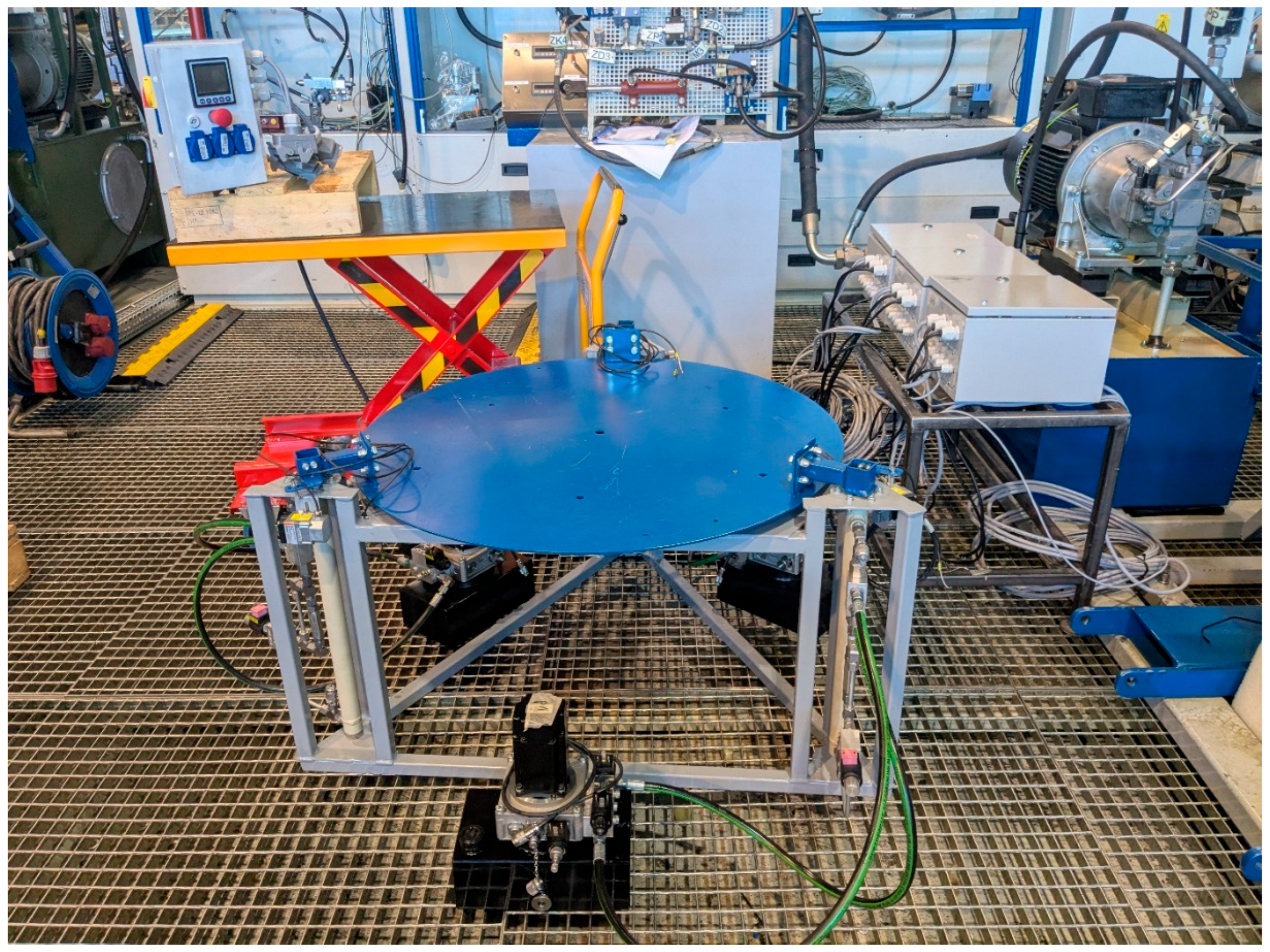
A three-module prototype of the modular architecture was built for experimental verification [60]. The number of modules was reduced from ten to three because three support points define a plane and therefore form a statically determinate arrangement: no redundant constraint can mask a synchronization error by redistributing load, so every difference between module strokes appears as a measurable tilt of the load plate. The three cylinders are spaced at 120° on a welded steel frame and carry a common circular load plate with radial mounting holes that allow the load to be displaced towards a chosen module; rod ends are articulated to avoid transverse constraint.

Each module uses a 0.75 kW servomotor driving a 0.26 cm³/rev gear pump and a cylinder with a 25 mm piston, an 18 mm rod and a 400 mm stroke, each cylinder loaded to 2.45 kN. On the 491 mm² piston area, that load corresponds to 50 bar, the upper end of the 11–50 bar working range of the rig, against 90 bar in the target device, so the pressure scale is λ_p = 50/90 = 0.556. The length scale is taken from the piston diameters, λ_L = 25/80 = 0.3125, which gives an area scale λ_A = 0.0977; the same scale obtained from the strokes, 400/1295 = 0.309, differs by 1.2%, confirming that the geometric scaling is consistent. The force scale follows as λ_Aλ_p = 0.054, confirmed by the ratio of nominal loads, 2.45 kN against 45.2 kN. Cylinder velocity ranges from about 14 mm/s at the nominal 1800 rpm of the servomotor to 24.4 mm/s at its maximum of 3000 rpm. The similarity achieved is geometric and static, not dynamic; the dynamic effects that the scaling distorts, and their consequences for transferring the results, are set out in Section Limitations and Transferability. The ratio of pump displacements gives a flow scale λ_Q = 0.26/1.2 = 0.217, hence a velocity scale λ_v = λ_Q/λ_A = 2.22 and a time scale λ_t = 0.309/2.22 = 0.139; both are confirmed directly by the measured quantities, 14.3 mm/s against 6.4 mm/s and 28 s against 201 s. Drift rates and transient lengths therefore do not transfer numerically, whereas quantities referred to the stroke do—which is why every synchronization result below is reported as a fraction of stroke. The rig is shown in Figure 2.

Position is measured by Kübler A41 draw-wire encoders (Fritz Kübler GmbH, Villingen-Schwenningen, Germany) with a 2000 mm range, ±0.15 mm repeatability and ±0.35% full-scale linearity, and pressure by IFM PT5401 transducers (ifm electronic gmbh, Essen, Germany) with a 0–250 bar range, 1 ms response and ±0.5% full-scale accuracy; pressure is recorded to verify the applied load and does not enter the control loop. Signals are acquired as 4–20 mA loops by a Horner XL4 OCS controller (Horner Automation Group, Indianapolis, IN, USA) with 12-bit analogue inputs and a 5–10 ms cycle. Twelve bits over the 2000 mm measuring range give 0.49 mm per bit, and with loop noise the effective position resolution is about ±1 mm; at the maximum velocity of 24.4 mm/s the 10 ms cycle corresponds to 0.24 mm of travel, well below that resolution. Speed setpoints are issued as 0–10 V, 16-bit signals to Astraada SRV-64 servo amplifiers (ASTOR, Kraków, Poland) whose inner loop closes on a 23-bit absolute encoder.

The quantity evaluated in the experiments is the difference between the positions of two modules, each measured by its own channel. Combining the specified error sources of the two channels formally—the linearity of the encoders (±0.35% of the 2000 mm full scale), the 1 mm resolution of the acquisition chain and the ±0.15 mm repeatability of the readings—gives an expanded uncertainty of about 11.5 mm at k = 2, almost all of it coming from the linearity term. This formal estimate is, however, far more pessimistic than the measurement it describes, for three reasons. The linearity error is systematic: it does not scatter randomly but varies slowly along the measuring range. Both channels use identical encoders and work over the same first fifth of that range, 0–400 mm out of 2000 mm, so a large part of the linearity error is the same in both channels and disappears when one reading is subtracted from the other. Whatever constant part remains is then removed by the calibration offset before each series. The resolution actually achieved by the measurement is shown by the data themselves: positions repeat between runs to 1.8–2.6 mm, independently determined quantities agree with one another, and both observations are consistent with the ±1 mm resolution of the acquisition chain. Steady-phase errors of 1.3–1.5 mm should therefore be read as indistinguishable from zero at the resolution of the measuring channel, while the verdicts on the ±8.0 mm band are unaffected, because every margin measured was far larger.

2.4. Synchronization Control

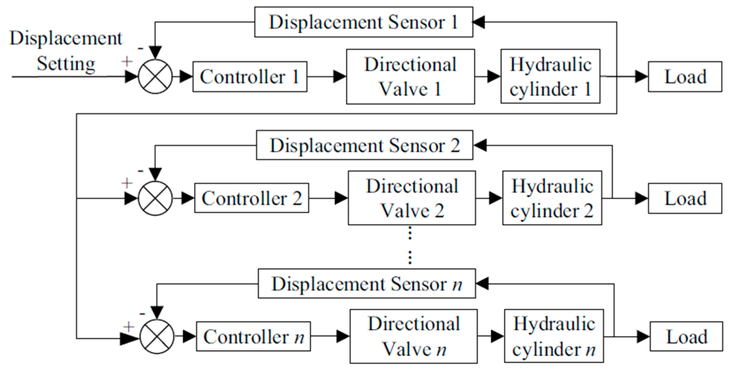
The three modules are synchronized by a two-level control structure. Each servo amplifier closes an inner speed loop on the 23-bit motor encoder of its drive, while the programmable logic controller closes an outer position loop on the draw-wire encoders within the 5–10 ms cycle given in Section 2.3. Module 1 is the master: its channel carries no controller and runs at a constant speed nm, 1800 rpm in every series, so that its motion defines the reference trajectory. Modules 2 and 3 are slaves and are corrected towards it. Figure 3 shows the structure.

The inner speed loop introduces a lag between the commanded and the actual pump speed, represented by a first-order element with the time constant T_s:

$${\displaystyle \frac{N_i\left(s\right)}{N_i^{\mathrm{s}\mathrm{e}\mathrm{t}}\left(s\right)}}={\displaystyle \frac{1}{T_{\mathrm{s}}s+1}}$$

(7)

with T_s = 0.05 s identified from the step responses of the drives. The synchronization error of slave i is the difference between the master and the slave position, corrected by the constant offset $e_{0,i}$ of its measuring channel:

$$e_i\left(t\right)=x_1\left(t\right)-x_i\left(t\right)-e_{0,i}$$

(8)

The error is quantized to q = 1 mm, the resolution of the acquisition chain, and the controller adds a proportional–integral–derivative correction to the master speed:

$$n_i^{\mathrm{s}\mathrm{e}\mathrm{t}}(t)=n_{\mathrm{m}}+K_{\mathrm{p}}{e}_i(t)+K_{\mathrm{i}}{\int }_0^t{e}_i\left(\tau \right)\mathrm{d}\tau +K_{\mathrm{d}}{\displaystyle \frac{\mathrm{d}{e}_i}{\mathrm{d}t}}$$

(9)

The commanded speed is then limited to the range of the drive:

$$0\le n_i^{\mathrm{s}\mathrm{e}\mathrm{t}}\le n_{\mathrm{m}\mathrm{a}\mathrm{x}}$$

(10)

The gains set in the controller were K_p = 40, K_i = 0 and K_d = 8. These numbers have no physical units, because the controller works in the internal units of the measuring channel and of the drive command, not in millimetres and rpm. The conversion is: 1 mm of error = 62.4 channel units; 1 command unit = 0.0915 rpm (32,767 units = 3000 rpm); K_p = 40 therefore adds about 228 rpm per millimetre of error, and one 1 mm step of the error—the resolution of the channel—moves the command by 2496 units, that is, by 228 rpm. The derivative parameter is entered in 10 ms units and acts as a derivative time, so K_d = 8 corresponds to T_d = 0.08 s, and the derivative term $T_{\mathrm{d}}{\displaystyle \frac{\mathrm{d}\mathrm{e}}{\mathrm{d}t}}$, computed against real time rather than per scan, contributes about 0.46 rpm for every 1 mm/s of error rate. The gains were not optimized. They were selected experimentally on the rig, before the sixteen-series programme, against a single requirement: that the closed-loop error stay within the ±2% band under the disturbance configurations of Section 2.5, including the combined one. K_d = 8 was set first to damp the start transient without introducing visible speed oscillation of the slaves; K_p was then raised from a low initial value until the ±2% requirement was met with a margin in the combined-disturbance case. The resulting value of 40 also satisfies two implementation constraints: it leaves the slaves a speed reserve of about 39% below saturation at the master speed of 1800 rpm, and it does not cause the command to alternate between adjacent quantization levels during the steady phase. No other criterion, such as minimum settling time or minimum RMS error, was applied, and a systematic tuning of the loop, including the integral term discussed below, is left to the full-scale device.

The integral gain was left at zero, so the controller works as a proportional–derivative one and the steady error derived below stays in the signal. This was intentional, for two reasons. First, that error grows with the loss of pump delivery, so it is exactly the quantity that the diagnostic rule of Section 3.5 makes use of; removing it would remove the symptom. Second, the command can only be corrected upwards, within the limit of Equation (10), and with such a one-sided limit an integral term would keep accumulating during the catch-up transients and then overshoot—the windup problem—unless an additional anti-windup scheme were implemented. What limits the loop in practice is not the gains but the speed reserve of about 39% noted above, which decides how much loss of pump delivery the loop can still make up for. Both choices are specific to this research prototype and were made so that the steady error remains visible as a diagnostic quantity; they are not a recommendation for a production device. A field version of the controller should carry the integral term, with anti-windup on the one-sided limit of Equation (10). The diagnostic information is not lost by that change: the same pump deficit then appears as a persistent offset in the integral term, that is, in the recorded control effort, instead of in the position error.

The derivative term acts on an error already quantized to 1 mm, and the recorded commands show what this means in practice. Through the steady phase, the quantized error keeps the same value for many controller cycles, so its change from one cycle to the next is zero, and the derivative adds nothing; the command then simply sits on one of the discrete levels spaced by K_pq. In two undisturbed lifting series, 96–99% of the recorded slave commands lie exactly on those levels, one quantization step apart; when the error jumps to the next millimetre, the derivative responds with a single-cycle spike, which the drive, with its 0.05 s time constant, averages out. On this rig, the behaviour was acceptable and is reported as measured; in a production version, the derivative should be filtered, or formed from a smoother estimate of the error rate, rather than left to be absorbed by the slow response of the drive.

The structure has one more consequence, and the measurements confirm it. In steady motion, the error does not change, so the derivative term is zero, and with K_i = 0, only the proportional part remains. Master and slave move at the same linear speed when k_v,1nm = k_v,ini^set; inserting the control law into this condition and solving for the error gives its steady value:

$$e_i^{\mathrm{s}\mathrm{s}}={\displaystyle \frac{n_{\mathrm{m}}}{K_{\mathrm{p}}}}{\displaystyle \frac{k_{\mathrm{v},1}-k_{\mathrm{v},i}}{k_{\mathrm{v},i}}}$$

(11)

Equation (11) has three practical consequences, taken up in Section 3.4: the steady error is proportional to the delivery that the slave pump has lost; raising K_p shrinks it only until quantization makes the command jump between widely spaced levels; and wear below the 1 mm resolution, invisible in positions, remains visible in the speed command, which the controller records anyway, with no additional sensor. This last point is why the integral term was left off: enabling it would drive the error of Equation (11) to zero and, with the error, erase the wear signature in the position readings.

2.5. Experimental Programme and Evaluation Criteria

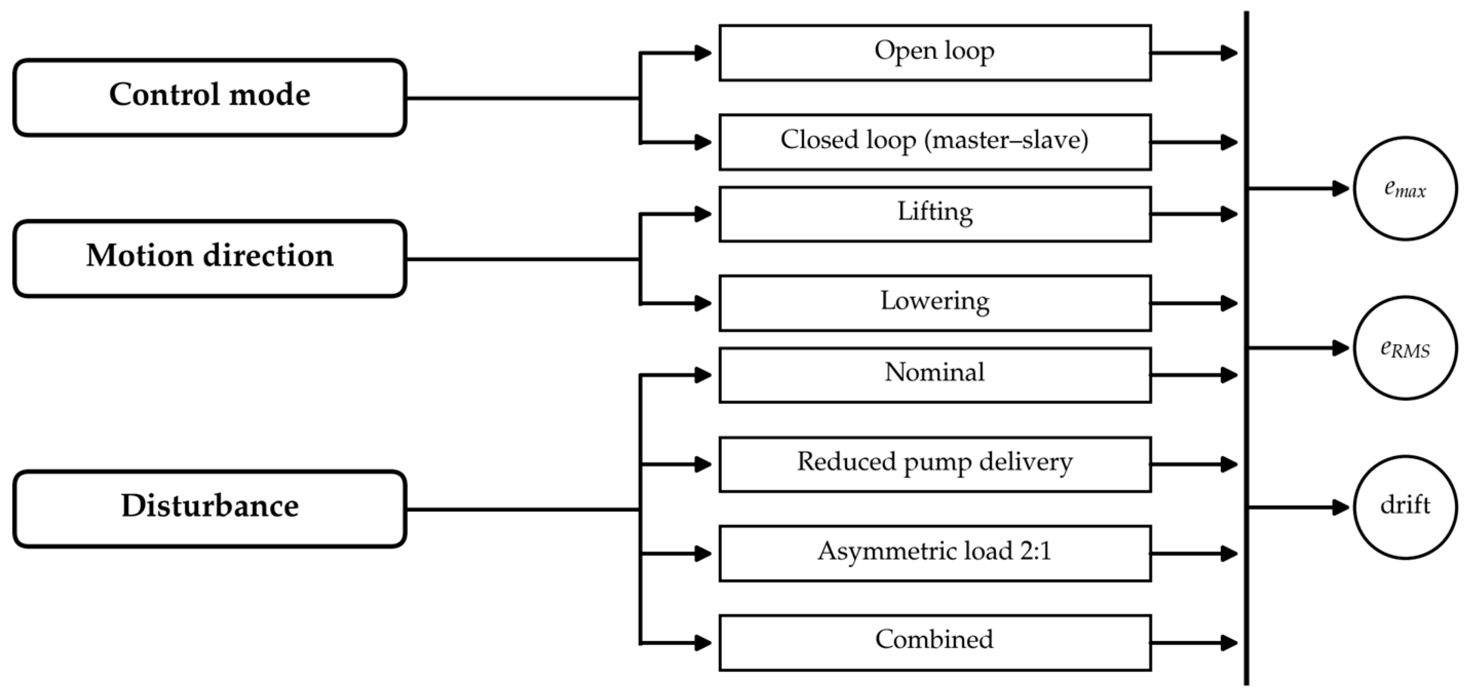
Sixteen series, S1–S16, form a full 2 × 2 × 4 factorial design in control mode, direction of motion and disturbance configuration, shown in Figure 4. The analysis was carried out on two levels: on the error curve averaged over the runs of each scenario (the ensemble curve, interpolated on a common 0.1 s grid), whose indicators are quoted in the text and tables, and on each run individually, which yields the run-to-run statistics. Every scenario was recorded in five runs, except S3 and S4 with four; no runs were excluded, so n in the tables of Section 3.3 and Section 3.4 equals the number of recorded runs. For every series, Tables of Section 3.3 and Section 3.4 report the ensemble indicator, the standard deviation of that indicator across the individual runs and the standard error of the ensemble regression slope; the individual-run values are available in the Supplementary Materials feedback, and the run-to-run dispersion of the position traces, taken as the mean standard deviation over the three channels, is 0.7–2.2 mm across the scenarios. With four to five runs per cell, no hypothesis tests are performed, and no confidence intervals are quoted; comparisons between series are stated as observations accompanied by their spread.

The control modes are:

• open loop, in which all three modules receive the same speed setpoint and no position feedback is applied—this is the feedback-free baseline of the modular prototype itself and the reference against which the benefit of closed-loop control is quantified. It shares with passive flow division the property that the cylinders receive a nominally equal, uncorrected flow, but it is not a measurement of the centralized architecture, as explained below;
• closed loop, in which module positions are measured, and modules 2 and 3 are corrected towards module 1, which runs at a constant speed as the master, by the control of Section 2.4.

The centralized variant was not tested physically; it was characterized from supplier documentation and functional analysis, and no experimental result in this paper refers to it directly. What the open-loop series share with passive flow division is functional: in both cases the cylinders receive a nominally equal flow set by positive displacement, no position feedback acts on the result, and the motion error is the time integral of whatever mismatch remains. That mismatch is of the same order in the two cases: a catalogue split accuracy of 2–5% for gear dividers of this class against a measured velocity spread of 3.3% between the nominally identical modules of the rig. What the open-loop series do not reproduce are the additional error sources of a real distribution network: hose compliance, leakage, and unequal loading of the divider sections, all of which act in the direction of a larger error in the centralized device. The open-loop results should therefore be read as the behaviour of a modular device without feedback, which is at the same time a favourable case of uncorrected flow division; they are not a measurement of the centralized variant, and the experimental comparison made in this paper is between open- and closed-loop operation of C3.

One difference between the rig and the centralized device is structural rather than parametric. In a gear flow divider, the sections sit on a common shaft, so a change in load at one outlet alters the pressure across that section, changes its internal leakage and affects every other outlet; on the rig, each module has its own pump and its own closed circuit, so a disturbance applied at one module stays there. The useful side of that coupling—all sections forced to a common speed—is reproduced on the rig, where every pump receives the same setpoint. Propagation of a disturbance between lifting points is not.

The rig therefore isolates the effect of each disturbance cleanly, which is what a factorial programme requires, but it cannot show how such a disturbance would spread in a centralized device. That propagation is very much the inter-module dependency the design structure matrix counts, and its absence from the rig is a further reason to expect the open-loop results to understate the error of the centralized architecture; the size of that understatement was not measured.

The four disturbance configurations are shown in Figure 4; two of them require a note on how they were realized.

• Reduced pump delivery was obtained by throttling the outlet of the pump of module 3. This reproduces the effect of pump wear on the delivered flow but not its mechanism: a worn pump shows pressure-dependent internal leakage, a volumetric efficiency that falls with load and temperature, and a nonlinear progression in time, whereas the throttle imposes a fixed loss of delivery. The disturbance is therefore called reduced pump delivery throughout, and the diagnostic rule of Section 3.5 is stated in those terms.
• The 2:1 load asymmetry was obtained by placing additional weights over one module so that its vertical support reaction is twice that of each of the others.

The quantity evaluated in every series is the difference in position between two modules. With three modules there are three such pairs, and the results are reported for the extreme pair, formed by the leading and the master module of the series concerned. Four indicators are derived from that signal: the maximum error e_max, its root mean square value e_RMS, the drift rate as the slope of a linear regression of error against time, and the fraction of stroke completed when the error first leaves the tolerance band.

Two evaluation windows are used. The full window covers the entire record, including the start transient, which lasts about one second in lifting and 1.1–1.2 s in lowering. The steady phase covers the constant-velocity part of the motion that follows it, and in lowering it covers the remaining 91–92% of the stroke. The maximum and the root mean square error are reported over both windows; the drift rate over the steady phase only.

The acceptance criterion is a synchronization error of ±2% of stroke, taken as the largest difference in position between any two lifting points, which corresponds to ±25.9 mm at the 1295 mm stroke of the target device and to ±8.0 mm at the 400 mm stroke of the rig. The band was not taken from a standard: it is an operational requirement specified for the device by the contractor that performs such erections, reflecting that company’s experience with tank lifting, and it is not a structural safety limit derived from the strength of the shell. Its engineering logic is nevertheless easy to trace. Passive synchronization by gear flow dividers is limited by internal leakage, by differences in the volumetric efficiency of the sections and by unequal loading of the actuators, which in practice give split errors between a fraction of a percent and a few percent [5,6,7]. A band of ±2% of stroke is therefore what well-maintained equipment of the current type can be expected to hold, and a replacement architecture has to hold at least the same.

A simple geometric check indicates that the band is compatible with the geometry of the lifted shell, although it does not establish a structural limit. With six to ten points on a 10–20 m tank, the permitted 25.9 mm difference tilts the supporting chord by at most about 1:200, the same order as the 1:200 out-of-plumbness that API 650 allows for the finished shell [62]. No standard covers the jacking phase itself, so this is a comparison of orders of magnitude, not a normative argument.

Where the criterion is met over the whole record, no band-exit value is reported. The effect of closed-loop control is quantified by a reduction factor, defined as the ratio of the open-loop to the closed-loop drift rate in absolute value for the matching pair of series and computed from unrounded values. Every run is documented by a measurement record containing the raw position traces of all three modules, the derived error signals, and the corresponding control effort.

A grey-box model was identified in MATLAB/Simulink R2026a (The MathWorks Inc., Natick, MA, USA) to separate the contributions of the individual mechanisms. Its structure follows the physics of the drive described in Section 2.4: cylinder velocity is proportional to servomotor speed through a coefficient k_v,i determined for each module, with a first-order lag and a transport delay. The coefficients, the time constant and the delay were identified on a subset of the series, and the model was then checked against further series from other disturbance configurations; therefore, the residuals reported in Section 3.5 come from series not used for identification.

2.6. Comparative Risk Assessment

A failure mode and effects analysis was carried out for the lifting function of both architectures. Hazard identification and the risk-reduction logic follow the general principles of ISO 12100 [16]; the analysis procedure and the risk priority number follow IEC 60812 [63]. The risk priority number RPN = S·O·D is used as the ranking measure, with severity S, occurrence O and detectability D scored on ten-point scales, so that RPN ranges from 1 to 1000. Severity is anchored to the consequence of losing position control at one lifting point, occurrence to the expected frequency of the initiating event per erection cycle, and detectability to whether the fault becomes observable before the position is lost.

The list of ten failure modes relevant to the lifting function was compiled from direct observation of the erection process and from the operating experience of the contractor that performs such work. The modes were then scored for both variants by expert judgement, using the same modes and the same scales for the two architectures. The scoring was carried out by the same team that established the dependency matrices of Section 2.2—the authors—whose experience spans the design of the modular variant, the manufacture of power units of the class analyzed and the erection practice in which both architectures operate, so the assessment is internal rather than independent, and its sensitivity to that fact is tested below. Severity was changed between the variants only where the architecture changes the consequence itself and not its likelihood, so the differences arise mainly from occurrence and detectability. The modes, their scores and their classification as low (RPN ≤ 80), medium (81–160), high (161–300) or critical (>300) are given in Section 3.6.

RPN is an ordinal expert-assigned indicator, and its products are not unique, so neither the individual values nor their sum is a measure of absolute risk, and the percentage change quoted below must not be read as an equivalent reduction in engineering risk. The values serve here as a common yardstick for two architectures assessed with the same modes, the same scales and the same panel. Expert subjectivity affects the absolute scores more than their difference—a systematic shift in the scales moves both variants together—but scores of this kind remain open to optimism bias in favour of the variant under development, so the comparison was tested against deliberate worsening of the modular scores rather than presented as a point estimate (Section 3.6).

3. Results

3.1. Functional Modules and Aggregated Dependency Structure

Table 1 lists the five modules of each architecture together with the elements assigned to them.

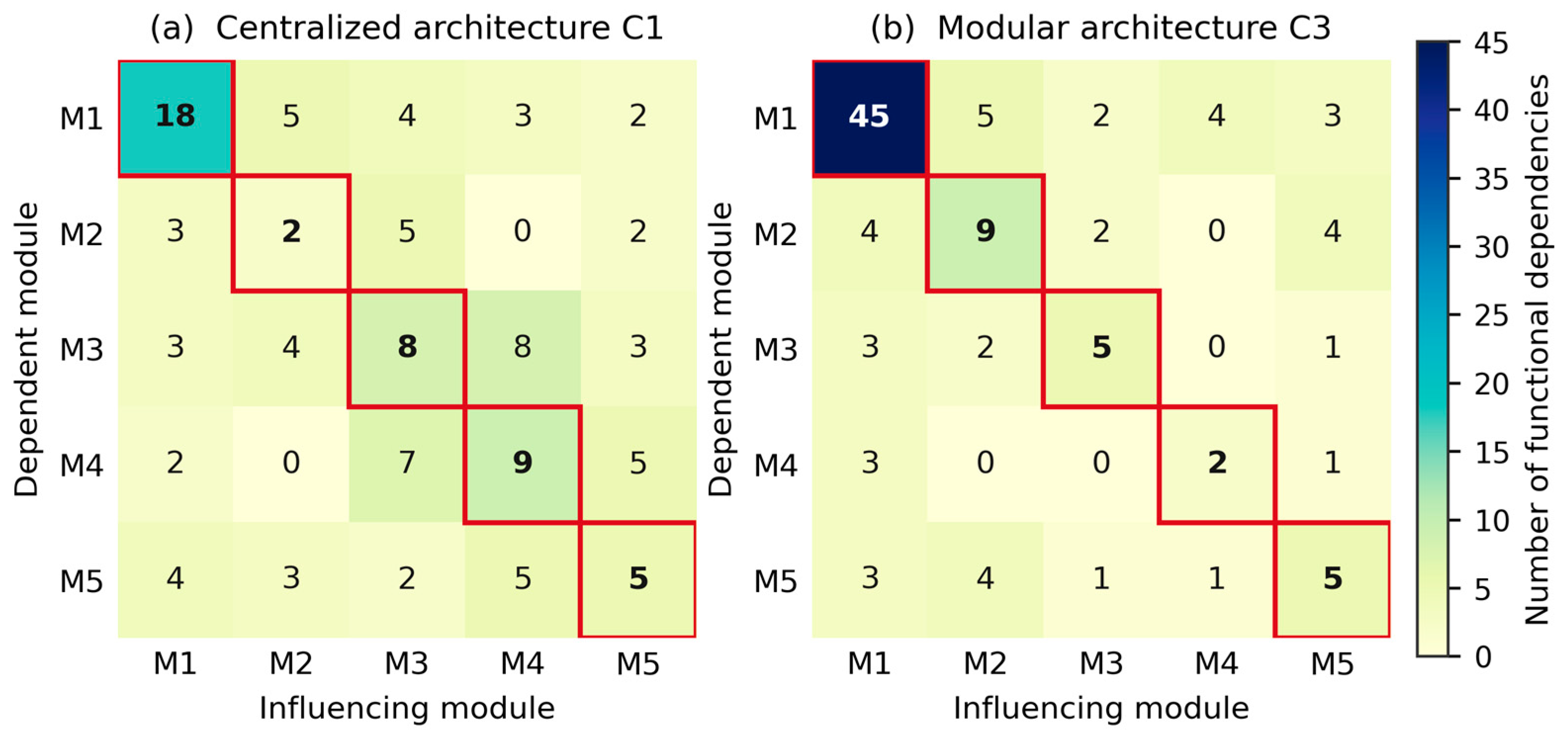
The two architectures contain almost the same total amount of structure: C1 has 21 elements linked by 112 directed dependencies, and C3 has 20 elements linked by 109. The difference is not in how much structure there is, but in where it sits. Figure 5 shows the dependencies summed up at the level of the five modules: the cells on the diagonal count the dependencies that stay inside a module, and the remaining cells count those that cross from one module to another.

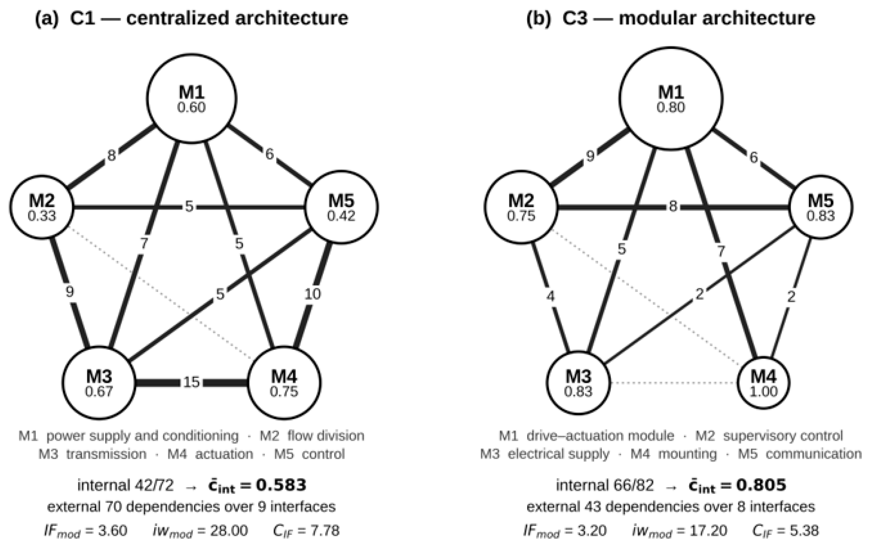
In C1, the internal dependencies total 42 against 70 crossing module boundaries; in C3, the ratio is reversed, with 66 internal against 43 external. The single largest change is in M1, which grows from six elements with 18 internal dependencies in C1 to eight elements with 45 internal dependencies in C3, because the modular architecture pulls the pump, the valve block, the reservoir, the cylinder and the sensor into one physical assembly. Only one pair of modules exchanges nothing in C1, namely M2 and M4; in C3, two pairs do; M2 with M4 and M3 with M4.

3.2. Modularity Indicators

The four indicators computed from the two matrices are collected in

Table 2. Modularity indicators of the two architectures, computed from the directed matrices according to Equations (1)–(5).

Indicator	Meaning	C1	C3	Change
${\overline{c}}_{\mathrm{i}\mathrm{n}\mathrm{t}}$	Mean internal cohesion (higher is better)	0.583	0.805	+38.1%
IFmod	Interfaces per module	3.60	3.20	−11.1%
iwmod	External dependencies per module	28.00	17.20	−38.6%
CIF	Mean interface complexity	7.78	5.38	−30.9%

Consistency check by Equation (6): 3.60 × 7.78 = 28.0 for C1 and 3.20 × 5.38 = 17.2 for C3.

; the per-module counts behind them are given in the Supplementary Materials.

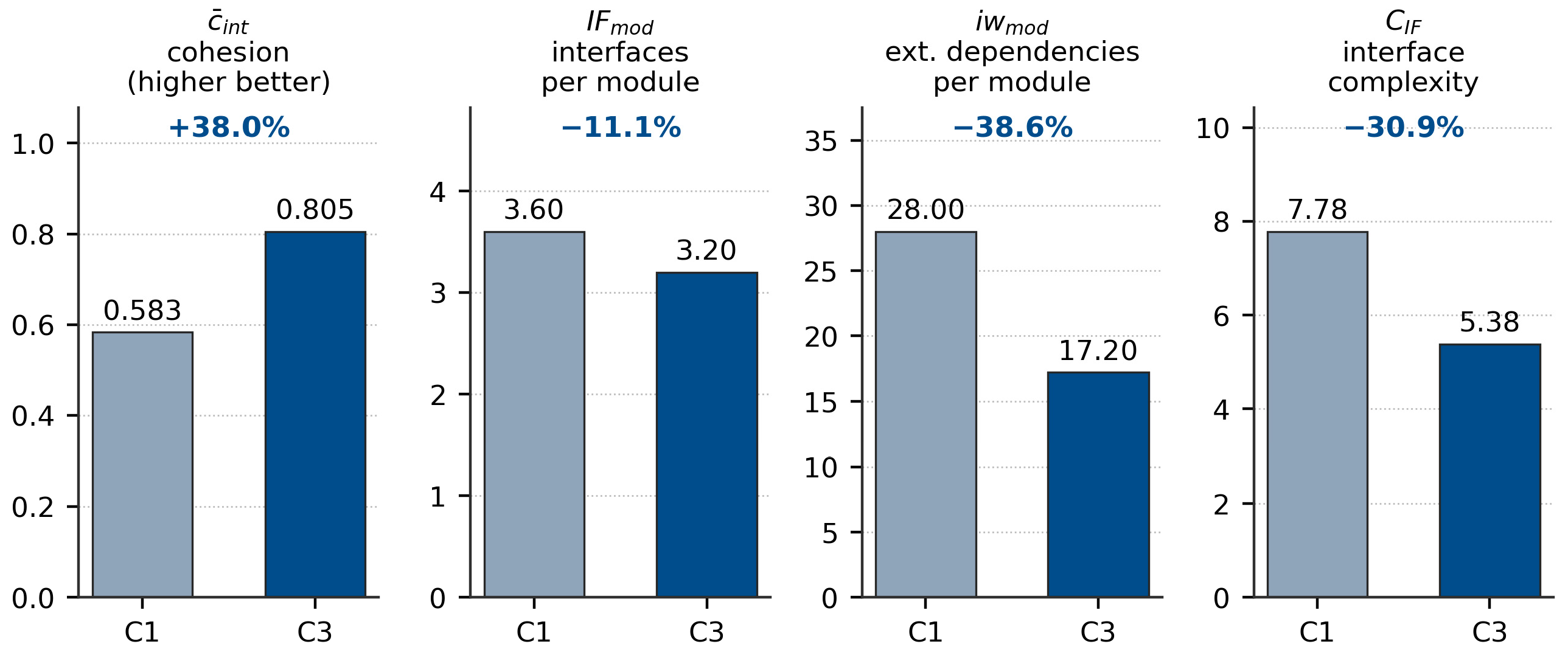
All four indicators move in the direction of greater modularity, and the identity of Equation (6) is satisfied for both matrices. The number of module pairs that must exchange something at all barely changes: IF_mod falls by only 11.1%, from 3.60 to 3.20, because the five functions still have to interact, whatever the physical arrangement. The traffic on each of those interfaces, by contrast, falls sharply—C_IF by 30.9% and, consequently, iw_mod by 38.6%. Modularization therefore reduced the content of the interfaces rather than their number. Figure 6 summarizes the four indicators, and Figure 7 shows the module-level dependency structure from which they are computed.

The whole computation was repeated on matrices in which a dependency in either direction was counted as a mutual coupling. This gives ${\overline{c}}_{\mathrm{i}\mathrm{n}\mathrm{t}}$ = 0.806 for C1 and 0.976 for C3 (+21.1%), iw_mod = 40.80 and 24.00 (−41.2%) and C_IF = 11.33 and 7.50 (−33.8%), with IF_mod unchanged at 3.60 and 3.20. The absolute values are different—they have to be, since every one-sided coupling is now counted twice—but the direction and the ranking of all four indicators stay the same. The conclusion therefore does not depend on how the matrix was built. Per-module cohesion values are given in the Supplementary Materials. The dependency counts behind these indicators can be verified from the complete matrices published in the Supplementary Materials, which also allow the indicators to be recomputed under alternative module assignments or after an independent re-coding of the dependencies by experts outside the author team; the sensitivity checks reported here bound the two choices that such a recomputation could vary—the matrix convention (symmetrization, above) and the deliberate worsening of the expert scores (Section 3.6).

3.3. Open-Loop Synchronization

The eight open-loop series are summarized in

Table 3. Open-loop synchronization indicators for the extreme module pair, referred to the 400 mm rig stroke. Percentages in parentheses are fractions of stroke. Values are indicators of the ensemble-averaged error curve over the n runs of the series; ± is the standard deviation of the same indicator computed for each run individually. No runs were excluded. Band exit is the first crossing of ±8.0 mm by the ensemble curve, as a percentage of the common motion window. The standard error of the ensemble regression slope is 0.004–0.013 mm/s across the series.

Series	Configuration	n	emax Δ(1−3) [mm]	eRMS Δ(1−3) [mm]	Drift Δ(1−3) [mm/s]	Band Exit [%]
S1	lifting, nominal	5	14.60 ± 0.55 (3.65%)	9.03 ± 0.40	+0.476 ± 0.007	46
S5	lifting, reduced pump delivery	5	19.60 ± 0.45 (4.90%)	12.06 ± 0.25	+0.660 ± 0.008	34
S9	lifting, 2:1 load asymmetry	5	15.60 ± 0.55 (3.90%)	9.69 ± 0.54	+0.514 ± 0.006	43
S13	lifting, combined	5	21.54 ± 0.45 (5.39%)	13.32 ± 0.43	+0.712 ± 0.010	33
S2	lowering, nominal	5	14.00 ± 1.34 (3.50%)	7.65 ± 1.33	−1.014 ± 0.044	60
S6	lowering, reduced pump delivery	5	14.60 ± 3.11 (3.65%)	7.93 ± 2.18	−1.106 ± 0.027	60
S10	lowering, 2:1 load asymmetry	5	14.06 ± 4.83 (3.52%)	7.69 ± 3.87	−0.980 ± 0.074	61
S14	lowering, combined	5	13.66 ± 4.10 (3.42%)	7.19 ± 3.25	−1.112 ± 0.115	63

, in each case for the extreme module pair.

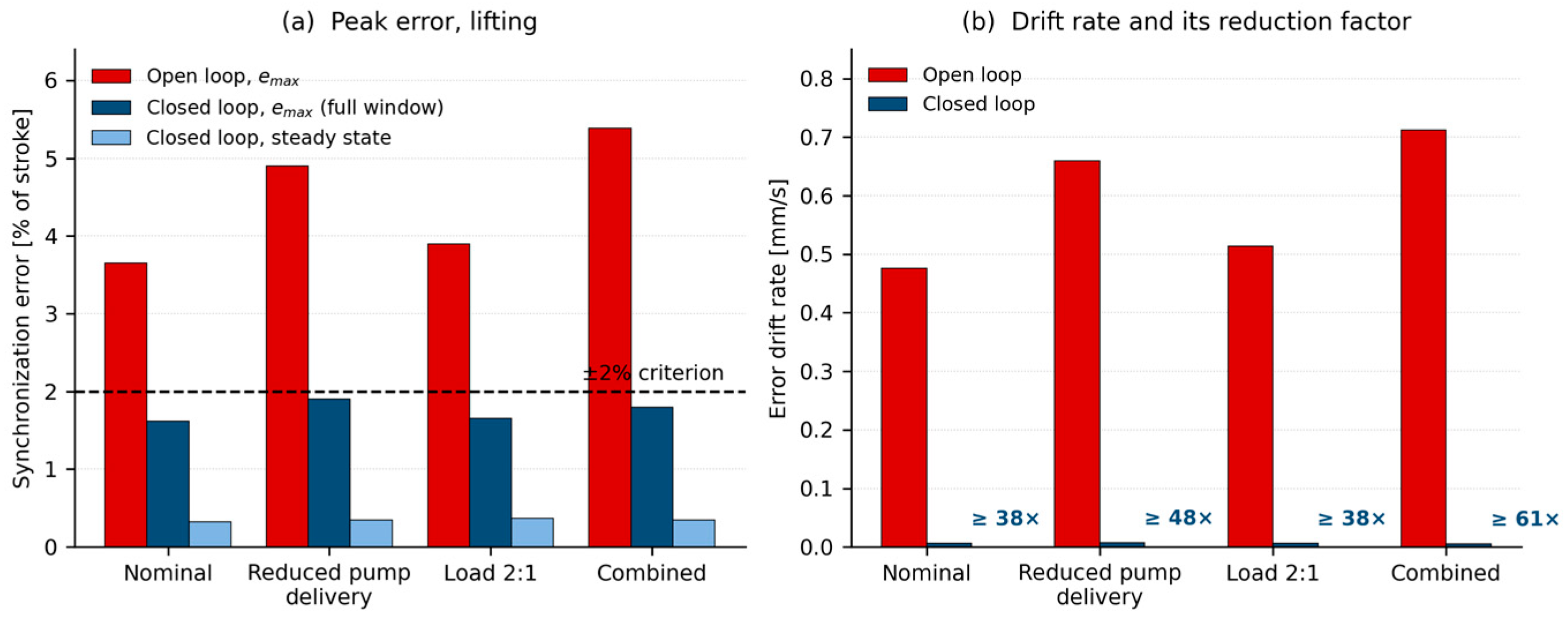
All eight open-loop series left the ±2% band: the lifting series after 33–46% of the motion window, the worst being the combined-disturbance case, and the lowering series after 60–63%. Even the nominal case was far from acceptable: with healthy pumps and a symmetric load, the extreme pair still drifted 14.60 mm apart, or 3.65% of stroke. The reason can be seen in the measured properties of the modules themselves. Their nominal velocities were 14.41, 14.10 and 13.93 mm/s, a spread of 3.3%, and this spread comes directly from the volumetric efficiencies of the pumps, 0.88 to 0.91, which differ by the same 3.3%: at equal displacement and equal speed the two spreads must be equal. Since the position error is simply the accumulated difference in the velocities, modules whose speeds differ by a few percent must end up a few percent of the stroke apart, whatever the stroke is.

Lowering is consistently worse than lifting: the drift rates, between 0.980 and 1.112 mm/s, are roughly twice as large. During descent, the load is driven by gravity, and the pilot-operated check valves open only after a certain pressure difference has built up, which adds a threshold behaviour of its own. The travel times of all twenty open-loop descents agree to within ±3% (13.2–14.1 s), but the drift itself varies between runs. Five of the twenty form a group with milder drift rates of −0.89 to −0.94 mm/s against −1.02 to −1.15 mm/s for the remaining fifteen, separated by a gap of 0.07 mm/s. The mild descents do not cluster in time within the measurement session, and their travel times, velocities and working pressures are indistinguishable from the rest, so the effect is treated as genuine run-to-run variability of the descent path, with the opening behaviour of the pilot-operated check valves as the plausible source. It accounts for most of the 2–10% run-to-run dispersion of the lowering drift rates and for the visibly larger dispersion of the lowering peak errors in Table 3. Nothing similar occurs in any lifting series (drift dispersion 1–2%); in closed loop the same one-sided character appears once: in one S16 descent with a drift of +0.37 mm/s against a typical +0.08 mm/s, and the loop keeps the error inside the band regardless, so the variability of the descent path is the disturbance that is the feedback.

3.4. Closed-Loop Synchronization

The eight closed-loop series are summarized in

Table 4. Closed-loop synchronization indicators. For lifting, the peak error occurs within the start transient; for lowering, the peak is the start transient itself, before the counterbalance valves of the slave modules open.

Series	Configuration	n	Peak Error, Full Window [mm]	emax, Steady Phase [mm] 2	Drift Δ(1−3) [mm/s]	Drift Reduction 3
S3	lifting, nominal	4	6.46 ± 0.95 (1.62%)	1.29 (0.32%)	−0.006 ± 0.002	≥38×
S7	lifting, reduced pump delivery	5	7.59 ± 0.44 (1.90%)	1.37 (0.34%)	−0.007 ± 0.003	≥48×
S11	lifting, 2:1 load asymmetry	5	6.62 ± 0.44 (1.66%)	1.46 (0.37%)	−0.006 ± 0.004	≥38×
S15	lifting, combined	5	7.19 ± 0.54 (1.80%)	1.38 (0.35%)	−0.005 ± 0.003	≥61×
S4	lowering, nominal	4	28.50 ± 0.58 (7.13%) 1	5.66 (1.42%)	+0.082 ± 0.038	12× ± 4
S8	lowering, reduced pump delivery	5	27.87 ± 0.80 (6.97%) 1	4.39 (1.10%)	+0.079 ± 0.068	14× ± 5
S12	lowering, 2:1 load asymmetry	5	25.62 ± 0.37 (6.41%) 1	5.65 (1.41%)	+0.049 ± 0.074	20× ± 10
S16	lowering, combined	5	25.30 ± 0.98 (6.33%) 1	5.18 (1.30%)	+0.022 ± 0.149	≥14×

¹ Transient peak on the pair Δ(1−2), the extreme pair of the start transient in every lowering series; the error re-enters the ±2% band permanently after 1.1–1.2 s, that is, after 8–9% of the motion window. ² Ensemble value; the extreme steady-phase pair is Δ(1−3) in S3, S7, S4 and S8 and Δ(1−2) in S11, S15, S12 and S16. Per-run steady maxima are higher (2.1–2.4 mm in lifting) because ensemble averaging smooths the ±1 mm quantization. ³ Ratio of the matching open- and closed-loop drift rates from unrounded values; where the closed-loop slope is indistinguishable from zero (|slope| ≤ 2 SE), the reduction is a lower bound computed with |slope| + 2 SE, and ± propagates the run-to-run SD of both drifts.

, with the reduction factor referred to the matching open-loop series.

In lifting, closed-loop control kept the error inside the ±2% band over the whole measurement window, start transient included. The largest error, 6.46–7.59 mm, appears about one second after the start—an unavoidable feature of master–slave control, which can react to an error only after that error has already been measured. Once the loop settles, the error drops to 1.29–1.46 mm, or 0.32–0.37% of stroke, and the drift practically stops: 0.005–0.007 mm/s, indistinguishable from zero at the resolution of the measuring chain and at least 38 to 61 times smaller than in the matching open-loop series (Figure 8).

In lowering, the picture differs in one respect only. Within the first 0.6 s, an error of 25.3–28.5 mm builds up on the pair Δ(1−2), and the reason is purely mechanical: the master starts moving immediately, while the slave modules cannot move at all until their valves open, and by then the master has already travelled 28–32 mm. The controller catches up, and the error returns to the band permanently after 8–9% of the motion window, staying at 4.39–5.66 mm, or 1.10–1.42% of stroke, over the remainder. The transient comes from the hydraulic holding circuit, not from the controller, and it is the reason why the reduction factor on descent, 12 to 20 times, is smaller than on ascent, where the closed-loop drift is indistinguishable from zero, and the reduction is at least 38–61-fold.

Referring to the stroke, the steady-phase errors of 0.32–0.37% in lifting and 1.10–1.42% in lowering lie well inside the ±2% criterion. No conversion of these values to millimetres of the target device is made, because the synchronization error arises from velocity mismatch and component dynamics, which do not scale with length (Section Limitations and Transferability). The effort needed to achieve this was small. The corrections stayed between +1.4% and +5.1% of the master setpoint, and the drives reached the 2500 rpm software limit only while catching up after the start, for 2–5% of the motion time, which leaves about 39% of speed reserve at the 1800 rpm master speed. The recorded commands also confirm the stepwise behaviour predicted in Section 2.4: the command of a slave alternates between levels 228 rpm apart, that is, by one 1 mm step of the position error. Averaged over the steady phase of two undisturbed lifting series, module 2 received +1.6–2.0% extra speed and module 3 received +2.9–3.1%, against pump deficits of 2.25% and 3.25% obtained from the velocity coefficients of Section 3.5. Dividing those corrections by the effective gain of 228.5 rpm/mm gives steady errors of 0.13–0.16 mm and 0.23–0.24 mm, against the 0.18 mm and 0.26 mm predicted by Equation (11). One caveat applies: the steady-phase error of 1.3–1.5 mm lies at the resolution limit of the measuring chain and is, in the sense of Section 2.3, indistinguishable from zero, so these values are upper bounds.

3.5. Superposition of Disturbances and Directional Signature

The additivity of the two disturbances is examined in

Table 5. Superposition of the individual disturbance contributions to the open-loop drift rate. Uncertainties are propagated from the standard errors of the ensemble regression slopes.

Direction	Base [mm/s]	Pump Increment [mm/s]	Load Increment [mm/s]	Predicted [mm/s]	Measured [mm/s]	Deviation
Lifting	+0.476	+0.184	+0.038	+0.698 ± 0.007	+0.712 ± 0.004	−1.9%
Lowering	−1.014	−0.092	+0.034	−1.073 ± 0.020	−1.112 ± 0.013	−3.5%

.

In lifting, the sum of the individually measured contributions predicts the combined case to within 1.9%, inside the combined uncertainty of the slopes. In lowering, the sum falls short of the measurement by 3.5%, against a combined standard uncertainty of about 2%, so the deviation is at the edge of what the present data resolve. Additivity of the two disturbances is therefore not contradicted in either direction, and a margin of about 10% on any predicted descent behaviour is retained as a prudent allowance.

The two directions also react to the two faults in opposite ways, and this is where the diagnostic value lies. In lifting, throttling the pump of module 3 raised the drift rate by 39%, while the 2:1 load asymmetry raised it by only 8%: in ascent, the pumps do the work, so ascent responds to the pumps. In lowering, the sensitivity flips. The same pump fault raised the drift rate by only 9%, and the correction demanded by the module with the throttled pump grew by a mere 0.4%—on descent the pump is almost invisible. The load asymmetry, by contrast, raised the peak error of the affected pair Δ(1−2) from 6.8 to 11.9 mm and doubled its RMS error, from 3.8 to 7.6 mm. In the nominal descent, that pair stays inside the ±2% band for the whole window; under the 2:1 asymmetry, it leaves the band after 63% because, in descent, gravity does the work and the counterbalance valve of the loaded module opens earlier. In terms of the factorial design of Section 2.5, this is a disturbance-by-direction interaction: the effect of each disturbance depends on the level of the direction factor. The practical rule follows directly: a loss of effective pump delivery is best assessed from lifting data and the condition of the holding valves from lowering data. The rule has been verified for an imposed loss of delivery only; a naturally worn pump adds pressure-dependent leakage, so its signature in the field is expected to be load-dependent rather than constant, and confirmation of the cause requires a separate measurement (Section Limitations and Transferability).

The grey-box model reproduces all of this. The identified velocity coefficients of the three modules are 0.00801, 0.00783 and 0.00775 mm·s⁻¹·rpm⁻¹; the velocities predicted from them agree with the measurements to better than 0.1%, and the error slopes of 0.33 and 0.48 mm/s are reproduced to within a few percent. The first-order lag with delay leaves a position residual of 0.47–0.58 mm root mean square in lifting and below 1.3 mm in lowering—on series that were not used for the identification. Two further checks support the model. Treating the velocity coefficients as constant is backed by observation: a pronounced redistribution of pressure between two open-loop runs left the cylinder velocities unchanged. In addition, the coefficients agree with the geometry of the drive: a 0.26 cm³/rev pump working on a 491 mm² piston gives 0.0088 mm·s⁻¹·rpm⁻¹, so the measured values correspond to a volumetric efficiency of about 0.91. The velocity spread of 3.3% quoted in Section 2.5 is the measured quantity, obtained from the open-loop regressions; the spread of volumetric efficiency is derived from it under the assumption of equal motor speed, so the two figures are not independent confirmations of each other.

3.6. Risk Assessment Results

The failure mode scores of the two architectures are compared in

Table 6. Failure mode and effects analysis of the lifting function: risk priority numbers for the centralized (C1) and modular (C3) architectures.

No.	Failure Mode	RPN C1	Level C1	RPN C3	Level C3	Reduction
1	Hydraulic hose rupture or loss of tightness	240	High	80	Low	66.7%
2	Incorrect hose connection	315	Critical	54	Low	82.9%
3	Working-fluid contamination during assembly	288	High	96	Medium	66.7%
4	Flow-divider damage or jamming	252	High	72	Low	71.4%
5	Loss of cylinder synchronization	350	Critical	90	Medium	74.3%
6	Uncontrolled lowering of a section	180	High	80	Low	55.6%
7	Loss of power supply	120	Medium	72	Low	40.0%
8	Position-sensor failure or loss of position information	168	High	63	Low	62.5%
9	Operator error during start-up or mode change	160	Medium	72	Low	55.0%
10	Pressure exceedance or section overload	180	High	81	Medium	55.0%
Σ	Total	2253	-	760	-	66.3%

.

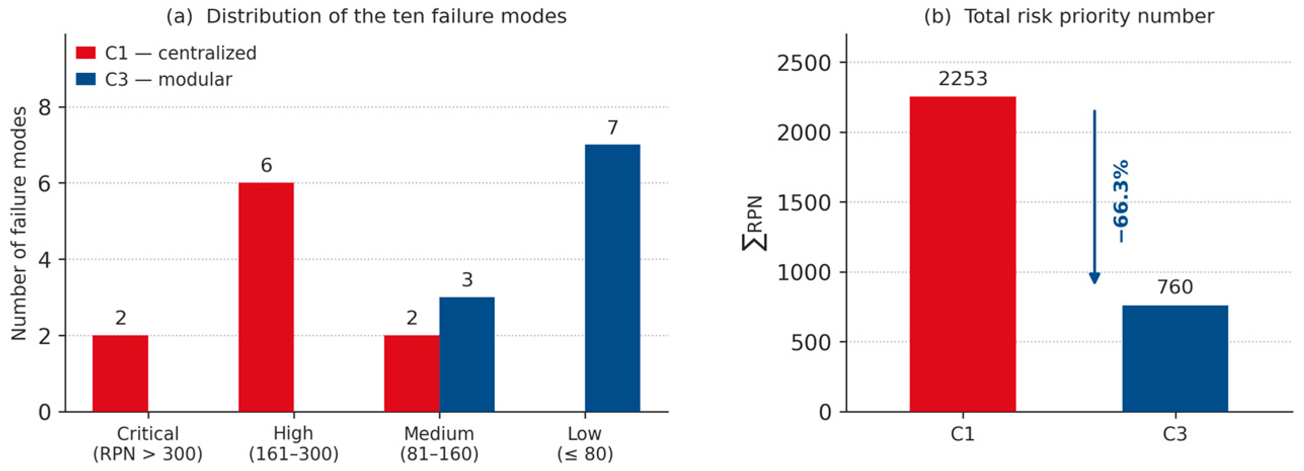
The total risk priority number falls from 2253 to 760, a reduction of 66.3% in this ordinal expert-assigned indicator, and the distribution changes qualitatively: C1 contains two critical, six high-risk and two medium-risk modes and no low-risk ones, whereas C3 contains no critical and no high-risk modes and seven low-risk ones (Figure 9). The largest relative reductions are for incorrect hose connection, loss of synchronization, and damage to the flow divider, all three rooted in the shared hydraulic installation.

The mechanism of the reduction is visible in the individual scores. Severity is almost unchanged: it is identical in nine of the ten modes and changes only for damage to the flow divider, an element the modular architecture does not contain. Loss of synchronization, for example, is scored 10·5·7 in C1 and 10·3·3 in C3, the severity of 10 being retained while occurrence and detectability improve. Severity is a property of the lifted load and of the consequences of dropping it, and no change in architecture can make a falling tank shell less severe. What architecture can change is how often the initiating event occurs and how early it is detected. Three mechanisms account for essentially all of the improvement: the elimination of long lines and of most detachable connections; the localization of the actuating and holding functions at the cylinder; and the presence of position measurement and diagnostic communication in every module. The last of these is not an assumption: the improvement in the detectability score for loss of synchronization follows from the demonstrated ability of the modular architecture to measure and correct the error continuously, and from the directional fault signatures reported in Section 3.5.

Because the scores are judgements, the comparison was checked against deliberate worsening of the modular ones rather than reported as a point estimate. Holding the detectability of the modular variant at the value assigned to the centralized one, that is, granting the modular architecture no benefit at all from local measurement, still leaves a total of 1431 against 2253, a reduction of 36.5%. Holding occurrence instead, so that the modular architecture is granted no reduction in the frequency of the initiating events, leaves 1192, a reduction of 47.1%. Penalizing both at once, by adding one point to every occurrence and every detectability score of the modular variant, gives 1368, a reduction of 39.3%, and the highest single value is then 160, so no failure mode reaches the high band even under that penalty. The sign and the order of magnitude of the comparison therefore do not depend on the precise scores, only on the direction of the changes, and that direction follows from the architecture itself: fewer detachable connections, load holding at the cylinder and position measurement in every module.

4. Discussion

The structural indicators and the measured behaviour point in the same direction, and the link between them is a concrete mechanism, not a correlation. The indicators iw_mod and C_IF measure the number of individual dependencies that cross module boundaries. In the centralized device, those dependencies are realized physically by the hydraulic installation and the flow divider—exactly the elements that carry the passive synchronization function, and exactly the elements that the failure mode analysis identifies as the dominant risk drivers. Reducing external dependencies by 38.6% is thus not an abstract improvement in a matrix: it is the removal of more than 300 m of hose, of the associated couplings and of the divider whose split accuracy previously determined the accuracy of the motion.

The relative size of the four changes are themselves informative. That IF_mod falls by only 11.1% while C_IF falls by 30.9% indicates that modularization did not eliminate the need for the five functions to interact; it reduced the number of individual dependencies realizing each interaction. For a device that is repeatedly assembled and disassembled under field conditions, this is the more valuable of the two effects, because the assembly time, the leakage risk and the number of parts to be handled attach to individual connections rather than to the abstract existence of an interface. An architecture with the same number of interfaces but thinner ones is substantially easier to erect and to service.

The cohesion indicator must be read with more care than the other three. Equation (2) rewards internal density, and the modular architecture concentrates eight elements in M1, so part of the increase from 0.583 to 0.805 follows from the definition of the indicator itself rather than from any real change in the design. This is why four indicators are reported together rather than one, why the identity of Equation (6) is used as an arithmetic check, and why the disjunctive symmetrization was computed: under that alternative convention the absolute values change considerably but the direction of all four indicators is preserved. Readers who prefer a different convention for building the matrix will obtain different numbers, but not a different conclusion. Metrics of this family are known to disagree with one another in individual cases [49,50], which is an argument for reporting the underlying counts, as is done in the Supplementary Materials, and not only the indicators.

Compared with the synchronization literature—tracking fluctuations of 0.19–0.27 mm [8,19] and below 0.1 mm with adaptive cross-coupling [22,23]—the steady-phase errors here, 1.29–1.46 mm, are large. The comparison is not like-for-like: the results reported here are obtained on three cylinders rather than two, with a deliberately imposed loss of pump delivery and a 2:1 load asymmetry rather than healthy components and a symmetric load, at considerably longer strokes, and through an acquisition chain whose ±1 mm resolution places the steady-phase error at the limit of what can be resolved. The informative result is not the absolute error, but its invariance: across four disturbance configurations the steady-phase error varied only between 1.29 and 1.46 mm, and the criterion was met throughout every lifting series. A control scheme whose performance is insensitive to the state of the components is worth more in field conditions than one that is excellent when everything is healthy.

The directional asymmetry is probably the most transferable finding of the experimental programme. Lifting and lowering do not. The structural gain corresponds to removing the hydraulic installation and the flow divider, which dominates both the open-differ in difficulty; they have different fault signatures, because in ascent the pumps do the work and in descent gravity does, with the counterbalance valves metering it. A loss of pump delivery that increases the ascent drift rate by 39% increases the descent drift rate by only 9%, while a load asymmetry that raises the ascent drift rate by only 8% roughly doubles the error of the affected pair in descent. This yields a diagnostic rule that requires no additional hardware in a device that already measures module positions: assess effective pump delivery from lifting data and holding valve condition from lowering data. Given the attention currently devoted to predictive maintenance of hydraulic components [54,55,57], a signature that is available from the normal working cycle without additional instrumentation is a practical asset.

Modularization is not free in engineering terms either. Replacing one central power unit with ten self-contained units multiplies the number of servo drives, power-electronic converters, local valve blocks and sensors, adds a communication network and a supervisory control programme that the centralized device does not need, and makes the lifting function dependent on an electrical supply at every lifting point rather than at one. This is the classical modularity trade-off [53] in a specific instance, and it is the reason why the structural indicators alone cannot decide between the two architectures: they measure how the dependencies are distributed, not how much apparatus is required to realize them. The penalty and the operational advantages that offset it are considered next, in directional terms only.

One dimension deliberately left outside the experimental programme is cost. A life-cycle cost comparison structured according to IEC 60300-3-3 [64] into acquisition, installation, energy, operation, maintenance, downtime, environmental and disposal costs, favours the centralized architecture in one category (acquisition) and the modular architecture in the remaining seven, the differences being driven by the extensive hydraulic installation, by throttling and flow splitting, by divider and hose wear, and by the immobilization of the whole system during a repair. Set against that, an order-of-magnitude estimate based on a supplier offer for the central power unit and on catalogue component prices puts the purchase price of the modular device about 58% higher. This is a directional comparison of categories and not a discounted cash-flow model: it does not establish a payback period, and whether the trade is worthwhile depends on utilization, since a device used for a few erections a year is dominated by its purchase price and one in continuous service by downtime.

Limitations and Transferability

The three lines of evidence do not have the same status. The structural indicators and the risk assessment compare C1 with C3 directly, but both rest on documentation and expert judgement. The experiments compare open- with closed-loop operation of the modular prototype only: the centralized variant was characterized from a device in commercial use, its technical documentation and a functional analysis, and was never tested. The open-loop series share with passive flow division the absence of position feedback, but they do not reproduce hose compliance, network leakage, and unequal loading of the divider sections, nor the coupling of those sections through a common shaft, all of which act towards a larger error (Section 2.5). Every statement about the performance of C1 in this paper is therefore an inference from those mechanisms and not a measurement; what the experiments establish is that closed-loop control removes almost all of the drift that uncorrected flow division produces on this rig.

The prototype reproduces the target device geometrically (λ_L = 0.3125) and statically (λ_p = 0.556) but not dynamically: it moves about twice as fast and completes its stroke in a seventh of the time. The effects this distorts are those with time constants of their own. The counterbalance and pilot-operated check valves open only after a pressure difference has built up, and that opening time occupies a larger fraction of the short rig stroke than it would at full scale, so the descent transient of 8–9% of the motion window is likely to be an upper bound. Fluid compressibility and line compliance are smaller in absolute terms in the short lines of the rig than in a 1295 mm cylinder at 90 bar, so the start of motion is stiffer on the rig than it will be in the field. Internal leakage of pumps, valves and cylinder seals grows with pressure, so at 90 bar the velocity mismatch between nominally identical modules, and with it the open-loop drift and the correction demanded in closed loop, will be larger than the 3.3% measured at 11–50 bar; the 39% speed reserve of Section 3.4 is the margin available for that increase. For these reasons, the errors are reported as fractions of stroke; no millimetre value is transferred to the target device, and the prototype results should be read as a favourable case that fixes the direction and the order of magnitude of the effects rather than their field values.

The rig has three modules and the target device ten. The master–slave structure scales linearly: each additional slave adds one position channel and one control loop; even for ten channels, the 5–10 ms controller cycle remains far below the drive time constant of 0.05 s and the 1–2 s transients. Communication does not accumulate either, because the speed setpoints are 0–10 V analogue outputs closed locally by the servo amplifiers and refreshed every cycle; a ten-module device needs ten analogue channels, and a fieldbus implementation, if preferred in the field, would add a per-node latency small compared with the same time constant. Because every module has its own closed circuit, there is no hydraulic path by which a disturbance at one lifting point can propagate to another, so the isolation observed with three modules does not deteriorate with ten. The mechanical coupling through the shell, however, does change: with more than three support points, the arrangement is statically indeterminate; the shell redistributes load between points, and partly masks position differences, and the number of module pairs grows to 45. The master-referenced error used here should then be complemented by a plane-fit or maximum-pairwise criterion referred to adjacent points. None of this has been tested; it is the object of the planned full-scale trial.

Each scenario was repeated five times (four in two scenarios), which supports the standard deviations, ranges and slope uncertainties now reported but not formal inference. The failure mode scores and the dependency matrices are expert judgements on common scales; they were checked by symmetrization and by deliberate worsening of the scores, which makes the comparisons internally consistent without making the absolute values meaningful outside them. The base pump speed was fixed throughout, so the interaction between synchronization and velocity profiling was not explored. Electrical energy consumption over a full working cycle was not measured, so the energy advantage of displacement control is argued from the literature [27,29,35] and from the elimination of throttling rather than demonstrated on this device. Finally, no reliability data from service, no results across the full temperature range, no certification, and no serial deployment exist yet, and the diagnostic rule has been verified only for a controlled, imposed loss of pump delivery, not for a naturally worn component.

Future work follows directly from those limitations: a full-scale ten-module device operating at 90 bar, a measured energy balance over a complete erection cycle, and naturally aged components for validating the diagnostic signatures. On the control side, the descent transient caused by the opening delay of the counterbalance valves is the obvious target: a feed-forward term derived from the measured valve characteristic should shorten it substantially, since it is a predictable effect.

5. Conclusions

(1) The centralized and modular variants of the same ten-cylinder lifting device contain almost the same amount of structure—112 against 109 directed dependencies—but distribute it very differently. Modularization raised the mean internal cohesion from 0.583 to 0.805 (+38.1%) and lowered the external dependencies per module by 38.6% and the mean interface complexity by 30.9%, while the number of interfaces per module fell by only 11.1%: modularization thinned the interfaces rather than removing them. The direction of all four indicators is independent of the matrix convention.

(2) Open-loop operation of the modular prototype, in which the modules receive a common speed command without position feedback, left the ±2—of-stroke band in all eight series—the lifting series after 33–46% of the motion window, the lowering series after 60–63%—and even the undisturbed lifting case reached 3.65% of stroke. A velocity spread of 3.3% between nominally identical modules is enough to produce this, because the position error is the accumulated difference in the velocities. The centralized variant was not tested; its behaviour is inferred from documentation and from the error mechanisms it shares with, and adds to, uncorrected flow division.

(3) Closed-loop master–slave control met the ±2% criterion over the whole window in the four lifting series, and over the last 91–92% of the motion window in the four lowering series, where a start transient set by the counterbalance valves exceeds the band. This holds under simultaneous reduced pump delivery and 2:1 load asymmetry as well, and in the present tests the error drift rate fell by one to two orders of magnitude: in lifting to below the resolution of the measuring chain (at least 38–61-fold), in lowering 12–20-fold. The steady-phase error was 0.32–0.37% of stroke in lifting and 1.10–1.42% in lowering, requiring correction amplitudes of at most 5.1% and leaving approximately 39% of speed reserve.

(4) Lifting and lowering have distinct fault signatures. A reduced pump delivery raises the ascent drift rate by 39% but the descent rate by only 9%, whereas a 2:1 load asymmetry raises the ascent drift rate by only 8% yet roughly doubles the error of the affected pair in descent. The effective delivery of the pumps should therefore be assessed from lifting data and holding valves from lowering data—a diagnostic rule that requires no additional hardware.

(5) The total risk priority number, an ordinal expert-assigned indicator, fell by 66.3%, from 2253 to 760, and no critical or high-risk failure mode remained in the modular architecture. The improvement comes from lower occurrence and better detectability, not from reduced severity, which is identical in nine of the ten failure modes—the expected and correct result for a lifting device.

Taken together, the results support the central methodological claim of the paper. The elements identified by the matrix as carrying the heaviest inter-module traffic are the same elements that the failure analysis identifies as the dominant risk drivers and the experiments identify as the source of drift—so an architecture-level indicator computed before construction pointed to what the hardware later showed to matter. The evidence rests on a single device and on a prototype at a length scale of 0.31, so the direction of the findings transfers more safely than their numerical values. It is also documentary rather than experimental for the centralized variant, so the comparison between the architectures is a structural and risk-based one, supported by a prototype test of the modular variant alone; and the modular device costs about 58% more to purchase, a premium that its operational advantages must repay. For a production version, the controller should carry an integral term with anti-windup, with the pump diagnostic read from the control effort rather than from the residual position error.

References

1. Ziółko, J.; Supernak, E.; Bąkowski, T. Stalowe zbiorniki walcowe pionowe—Metody ich montażu stosowane w Polsce od drugiej połowy XX wieku. Inż. Bud. 2018, 74, 445–451. [Google Scholar]
2. Budkiewicz, Z.; Jereczek, P.; Mikulski, T. Montaż płaszczy osłonowych i zbiorników stalowych metodą podbudowy [Erection of Shielding Shells and Steel Tanks by the Jacking-Up Method]. Inż. Bud. 2007, 63, 570–572. [Google Scholar]
3. Zamorowski, J.; Gremza, G. A System Consists of Lifted Steel Tank and Four Assembly Supports with Variable Assembly Conditions. SGEM 2018, 40, 263–269. [Google Scholar] [CrossRef] [Scilit]
4. Kamran, H.; Komasi, M.; Mousavi, S.H. Optimization and Simulation of Fluid Reservoirs under Seismic Loads Using Finite Element Analysis and Artificial Neural Networks. J. Civ. Eng. Mater. Appl. 2025, 9, 111–124. [Google Scholar] [CrossRef]
5. Rybak, A.; Meskhi, B.; Rudoy, D.; Olshevskaya, A.; Teplyakova, S.; Kolesnikov, I.; Prutskov, A. Test Bench for Throttle Flow Dividers-Adders. BIO Web Conf. 2024, 113, 05016. [Google Scholar] [CrossRef] [Scilit]
6. Kumar, D.; Mahato, A.C.; Prakash, O.; Kumar, K. Priority Flow Divider Valve and Its Dynamic Analysis Using Various Hydraulic Drive Systems: A Bond Graph Approach. Mech. Sci. 2022, 13, 459–472. [Google Scholar] [CrossRef] [Scilit]
7. Hradecký, J.M. Description of Pressure-Multiplying Efficiency Model Creation Used for Pressure Intensifiers Based on Rotary Flow Dividers. Energies 2023, 16, 4014. [Google Scholar] [CrossRef] [Scilit]
8. Li, K.; Chen, J.; Xiao, Z.; Xu, M. An Electrohydraulic System for Synchronized Roof Erection. Autom. Constr. 2003, 12, 29–42. [Google Scholar] [CrossRef] [Scilit]
9. Zardin, B.; Cillo, G.; Rinaldini, C.; Mattarelli, E.; Borghi, M. Pressure Losses in Hydraulic Manifolds. Energies 2017, 10, 310. [Google Scholar] [CrossRef] [Scilit]
10. Singh, M.; Lathkar, G.; Basu, S. Failure Prevention of Hydraulic System Based on Oil Contamination. J. Inst. Eng. Ser. C 2012, 93, 269–274. [Google Scholar] [CrossRef] [Scilit]
11. Sharma, A.; Kumar, N.; Das, A. A Review on Wear Failure of Hydraulic Components: Existing Problems and Possible Solutions. Eng. Res. Express 2024, 6, 012502. [Google Scholar] [CrossRef] [Scilit]
12. Novak, N.; Trajkovski, A.; Kalin, M.; Majdič, F. Degradation of Hydraulic System Due to Wear Particles or Medium Test Dust. Appl. Sci. 2023, 13, 7777. [Google Scholar] [CrossRef] [Scilit]
13. Xing, Y.; Zhai, F.; Li, S.; Wang, X.; He, Z. A Study on Radial Oil Seal Leakage Failure Due to Viscoelasticity under Dynamic Eccentricity. ILT 2024, 76, 1197–1204. [Google Scholar] [CrossRef] [Scilit]
14. Dindorf, R. Bezpieczeństwo Układów Hydraulicznych i Pneumatycznych; Wydawnictwo Politechniki Świętokrzyskiej: Kielce, Poland, 2018; ISBN 978-83-65719-24-9. [Google Scholar]
15. Locking Protection is Key to Hydraulic System Safety. Fluid Power Journal. Available online: https://fluidpowerjournal.com/ (accessed on 27 June 2026).
16. ISO 12100:2010; Safety of Machinery-General Principles for Design-Risk Assessment and Risk Reduction. International Organization for Standardization: Geneva, Switzerland, 2010.
17. Yan, K.; Jin, L.; Yu, X. Ordered Weighted Evaluation Method of Lifting Operation Safety Risks Considering Coupling Effect. Sci. Rep. 2024, 14, 5776. [Google Scholar] [CrossRef] [Scilit] [PubMed]
18. Del Giudice, M.E.; Sharafkhani, M.; Di Nardo, M.; Murino, T.; Leva, M.C. Exploring Safety of Machineries and Training: An Overview of Current Literature Applied to Manufacturing Environments. Processes 2024, 12, 684. [Google Scholar] [CrossRef] [Scilit]
19. Meena, K.; Dhavalikar, M.; Thorat, S. A Review on the Position Control of Hydraulic Cylinder for Accuracy and Response Time. Mater. Today Proc. 2023, 72, 995–999. [Google Scholar] [CrossRef] [Scilit]
20. Wang, J. Hydraulic Synchronization Control Research Status and Outlook. J. Eng. Res. Rep. 2024, 26, 458–470. [Google Scholar] [CrossRef] [Scilit]
21. Liu, L.P. Dual Hydraulic Cylinders Synchronized Control Strategy. Adv. Mater. Res. 2014, 898, 546–549. [Google Scholar] [CrossRef] [Scilit]
22. Sun, C.; Dong, X.; Li, J. Cross-Coupled Sliding Mode Synchronous Control for a Double Lifting Point Hydraulic Hoist. Sensors 2023, 23, 9387. [Google Scholar] [CrossRef] [Scilit] [PubMed]
23. Sun, H.; Chiu, G.T.-C. Motion Synchronization for Dual-Cylinder Electrohydraulic Lift Systems. IEEE/ASME Trans. Mechatron. 2002, 7, 171–181. [Google Scholar] [CrossRef]
24. Woś, P.; Dindorf, R. Synchronization of the Movement for Multi-Cylinder Electrohydraulic Servo Driver. EPJ Web Conf. 2022, 269, 01069. [Google Scholar] [CrossRef] [Scilit]
25. Xue, Y.; Wang, B.; Xu, J.; Sun, Q.; Zhang, P. Research on Multi-Cylinder Coordinated Coupling Synchronous Control Strategy Based on Strain Energy. Sci. Rep. 2025, 15, 44277. [Google Scholar] [CrossRef] [Scilit] [PubMed]
26. Wang, J.; Hao, S.; Li, W. Study on Multiple Hydraulic Cylinders Synchronous Control Under Impact Load. In The 8th International Conference on Advances in Construction Machinery and Vehicle Engineering; Halgamuge, S.K., Zhang, H., Zhao, D., Bian, Y., Eds.; Lecture Notes in Mechanical Engineering; Springer Nature: Singapore, 2024; pp. 505–518. ISBN 978-981-97-1875-7. [Google Scholar]
27. Vukovic, M.; Murrenhoff, H. The Next Generation of Fluid Power Systems. Procedia Eng. 2015, 106, 2–7. [Google Scholar] [CrossRef] [Scilit]
28. Mahato, A.C.; Ghoshal, S.K. An Overview of Energy Savings Approaches on Hydraulic Drive Systems. Int. J. Fluid Power 2020, 21, 81–118. [Google Scholar] [CrossRef] [Scilit]
29. Alemdaroglu, U.; Guler, Z.; Sevim, S.; Dalkiran, F. Energy Efficiency by Reducing Throttling Losses in Hydraulic Systems. J. Mechatron. Artif. Intell. Eng. 2023, 4, 1–7. [Google Scholar] [CrossRef] [Scilit]
30. Gao, G.; Wen, J.; Liu, X.; Zhang, Z. Synchronous Smooth Sliding Mode Control for Parallel Mechanism Based on Coupling Analysis. Int. J. Adv. Robot. Syst. 2013, 10, 173. [Google Scholar] [CrossRef] [Scilit] [PubMed]
31. Milecki, A.; Jakubowski, A.; Kubacki, A. Design and Control of a Linear Rotary Electro-Hydraulic Servo Drive Unit. Appl. Sci. 2023, 13, 8598. [Google Scholar] [CrossRef] [Scilit]
32. Yan, G.; Jin, Z.; Zhang, T.; Zhang, C.; Ai, C.; Chen, G. Exploring the Essence of Servo Pump Control. Processes 2022, 10, 786. [Google Scholar] [CrossRef] [Scilit]
33. Chen, G.; Jia, P.; Yan, G.; Liu, H.; Chen, W.; Jia, C.; Ai, C. Research on Feedback-Linearized Sliding Mode Control of Direct-Drive Volume Control Electro-Hydraulic Servo System. Processes 2021, 9, 1676. [Google Scholar] [CrossRef] [Scilit]
34. Stawiński, Ł.; Kosucki, A.; Skowrońska, J.; Malenta, P. Energy Efficiency Improvement of Hydraulic Indirect Elevator. Energies 2025, 18, 2163. [Google Scholar] [CrossRef] [Scilit]
35. Qu, S.; Fassbender, D.; Vacca, A.; Busquets, E. A High-Efficient Solution for Electro-Hydraulic Actuators with Energy Regeneration Capability. Energy 2020, 216, 119291. [Google Scholar] [CrossRef] [Scilit]
36. Quan, Z.; Ge, L.; Wei, Z.; Li, Y.W.; Quan, L. A Survey of Powertrain Technologies for Energy-Efficient Heavy-Duty Machinery. Proc. IEEE 2021, 109, 279–308. [Google Scholar] [CrossRef] [Scilit]
37. Li, R.; Zhang, Y.; Feng, Z.; Xu, J.; Wu, X.; Liu, M.; Xia, Y.; Sun, Q.; Yuan, W. Review of the Progress of Energy Saving of Hydraulic Control Systems. Processes 2023, 11, 3304. [Google Scholar] [CrossRef] [Scilit]
38. Ulrich, K. The Role of Product Architecture in the Manufacturing Firm. Res. Policy 1995, 24, 419–440. [Google Scholar] [CrossRef] [Scilit]
39. Pahl, G.; Beitz, W.; Feldhusen, J.; Grote, K.-H. Engineering Design: A Systematic Approach, 3rd ed.; Wallace, K., Blessing, L., Eds.; Springer: London, UK, 2007; ISBN 978-1-84628-318-5. [Google Scholar]
40. Erixon, G. Modular Function Deployment-A Method for Product Modularisation. Ph.D. Thesis, Royal Institute of Technology (KTH), Stockholm, Sweden, 1998. [Google Scholar]
41. Levandowski, C.; Müller, J.R.; Isaksson, O. Modularization in Concept Development Using Functional Modeling. In Advances in Transdisciplinary Engineering; IOS Press: Amsterdam, The Netherlands, 2016. [Google Scholar]
42. Baldwin, C.Y.; Clark, K.B. Modularity in the Design of Complex Engineering Systems. In Complex Engineered Systems: Science Meets Technology; Braha, D., Minai, A.A., Bar-Yam, Y., Eds.; Springer: Berlin/Heidelberg, Germany, 2006; pp. 175–205. ISBN 978-3-540-32834-6. [Google Scholar]
43. Pakkanen, J.; Juuti, T.; Lehtonen, T.; Mämmelä, J. Why to Design Modular Products? Procedia CIRP 2022, 109, 31–36. [Google Scholar] [CrossRef] [Scilit]
44. Browning, T.R. Applying the Design Structure Matrix to System Decomposition and Integration Problems: A Review and New Directions. IEEE Trans. Eng. Manag. 2001, 48, 292–306. [Google Scholar] [CrossRef] [Scilit]
45. Pimmler, T.U.; Eppinger, S.D. Integration Analysis of Product Decompositions. In Proceedings of the ASME 1994 Design Technical Conferences, Minneapolis, MN, USA, 11–14 September 1994; pp. 343–351. [Google Scholar]
46. Sinha, K.; Han, S.; Suh, E.S. Design Structure Matrix-based Modularization Approach for Complex Systems with Multiple Design Constraints. Syst. Eng. 2020, 23, 211–220. [Google Scholar] [CrossRef] [Scilit]
47. Wang, S.; Li, Z.; He, C.; Liu, D.; Zou, G. An Integrated Method for Modular Design Based on Auto-Generated Multi-Attribute DSM and Improved Genetic Algorithm. Symmetry 2022, 14, 48. [Google Scholar] [CrossRef] [Scilit]
48. Jung, S.; Simpson, T.W. New Modularity Indices for Modularity Assessment and Clustering of Product Architecture. J. Eng. Des. 2016, 28, 1–22. [Google Scholar] [CrossRef] [Scilit]
49. Guo, F.; Gershenson, J.K. Comparison of Modular Measurement Methods Based on Consistency Analysis and Sensitivity Analysis. In Proceedings of the ASME 2003 International Design Engineering Technical Conferences, Chicago, IL, USA, 2–6 September 2003; pp. 393–401. [Google Scholar] [CrossRef] [Scilit]
50. Cheng, X.; Wan, C.; Qiu, H.; Luo, J. A Measure for Modularity and Comparative Analysis of Modularity Metrics. In Proceedings of the 24th International Conference on Industrial Engineering and Engineering Management 2018; Huang, G.Q., Chien, C.-F., Dou, R., Eds.; Springer: Singapore, 2019; pp. 266–277. [Google Scholar]
51. Fortunato, S. Community Detection in Graphs. Phys. Rep. 2010, 486, 75–174. [Google Scholar] [CrossRef] [Scilit]
52. Newman, M. Networks, 2nd ed.; Oxford University Press: Oxford, UK, 2018; ISBN 978-0-19-880509-0. [Google Scholar]
53. Hölttä, K.; Suh, E.S.; de Weck, O. Tradeoff Between Modularity and Performance for Engineered Systems and Products. In Proceedings of the International Conference on Engineering Design (ICED 05), Melbourne, Australia, 15–18 August 2005. [Google Scholar]
54. Rivera, D.; Scholz, M.; Fritscher, M.; Krauss, M.; Schilling, K. Towards a Predictive Maintenance System of a Hydraulic Pump. IFAC-PapersOnLine 2018, 51, 447–452. [Google Scholar] [CrossRef] [Scilit]
55. Sharma, A.; Punj, P.; Kumar, N.; Das, A.; Kumar, A. Lifetime Prediction of a Hydraulic Pump Using ARIMA Model. Arab. J. Sci. Eng. 2023, 49, 1713–1725. [Google Scholar] [CrossRef] [Scilit]
56. Araste, Z.; Sadighi, A.; Jamimoghaddam, M. Fault Diagnosis of a Centrifugal Pump Using Electrical Signature Analysis and Support Vector Machine. J. Vib. Eng. Technol. 2022, 11, 2057–2067. [Google Scholar] [CrossRef] [Scilit]
57. Zakharov, V.; Huynh, V.K.; Minav, T. AI-Based Hydraulic and Electrical Fault Identification in Direct-Driven Hydraulic Systems. IEEE Access 2026, 14, 4940–4952. [Google Scholar] [CrossRef] [Scilit]
58. Becker, M.; Karaoglu, S.; Makansi, F.; Radtke, J.; Schmitz, K. Industry 4.0: Review of the State of the Art in Fluid Power Research and Industry. Int. J. Fluid Power 2025, 26, 573–624. [Google Scholar] [CrossRef] [Scilit]
59. Żuczek, A.; Rząsiński, R. The Concept of an Energy-Efficient, Modular Hydraulic Device That Increases Work Safety and Reduces Labor Intensity in the Construction of Large-Scale Structures in Field Conditions. In Proceedings of the Intelligent Systems in Production Engineering and Maintenance III; Burduk, A., Batako, A.D.L., Machado, J., Wyczółkowski, R., Dostatni, E., Rojek, I., Eds.; Springer Nature: Cham, Switzerland, 2024; pp. 615–626. [Google Scholar] [CrossRef] [Scilit]
60. Żuczek, A.; Rząsiński, R. Synchronization of Hydraulic Actuators Motion in an Energy-Efficient, Modular Hydraulic Device: Concept of Device and Construction of a Test Stand. In Proceedings of the Intelligent Systems in Production Engineering and Maintenance IV; Burduk, A., Janmanee, P., Batako, A.D.L., Patalas-Maliszewska, J., Dostatni, E., Kochańska, J., Wyczółkowski, R., Eds.; Springer Nature: Cham, Switzerland, 2026; pp. 140–153. [Google Scholar] [CrossRef] [Scilit] [PubMed]
61. Salerno, F.; Ulrich, L.; Maculotti, G.; Moos, S.; Genta, G.; Vezzetti, E.; Galetto, M. A Metrological Approach for Augmented Reality Tooltip Tracking Assessment. Comput. Ind. 2026, 175, 104430. [Google Scholar] [CrossRef] [Scilit]
62. API 650-Plumbness Tolerance for One Shell. Available online: https://www.eng-tips.com/threads/api-650-plumbness-tolerance-for-one-shell.460434/ (accessed on 21 August 2026).
63. IEC 60812:2018; Failure Modes and Effects Analysis (FMEA and FMECA). International Electrotechnical Commission: Geneva, Switzerland, 2018.
64. IEC 60300:2017; Dependability Management—Part 3-3: Application Guide—Life Cycle Costing. International Electrotechnical Commission: Geneva, Switzerland, 2017.
Figure 1. The compared concepts of the lifting device: (a) photograph of a power unit of the centralized concept C1 with the gear flow divider; (b) visualization of the C1 field installation at the tank; (c) model of the autonomous module of the modular concept C3; (d) visualization of the corresponding C3 installation.
Applsci 16 09092 g001
Figure 2. Three-module prototype of the modular lifting device: three cylinders at 120° under a common load plate, each with its own servomotor-driven power module.
Applsci 16 09092 g002
Figure 3. Two−level master−slave synchronization structure: the master runs at constant speed without a controller, while each slave adds a correction, formed from its position error against the master, to the master speed.
Applsci 16 09092 g003
Figure 4. Factorial structure of the experimental programme: two control modes × two directions of motion × four disturbance configurations, giving sixteen series. The three main response variables are shown; the fraction of stroke at band exit is derived from the same records [61].
Applsci 16 09092 g004
Figure 5. Module-level aggregation of the directed design structure matrices: (a) centralized architecture C1; (b) modular architecture C3. Rows are dependent modules, columns are influencing modules; diagonal cells, outlined in red, contain dependencies internal to a module.
Applsci 16 09092 g005
Figure 6. Modularity indicators of the centralized (C1) and modular (C3) architectures, with the relative change annotated above each pair of bars.
Applsci 16 09092 g006
Figure 7. Module-level dependency graph of the two architectures: (a) centralized C1; (b) modular C3. Node area is proportional to the number of functional elements assigned to the module and the value inside each node gives its internal cohesion cint,k of Equation (1); edge width and the adjacent number give the number of directed dependencies crossing that module pair, and a dashed line marks a pair with no interface at all. The graph is the module-level aggregation of Figure 5, read as a network.
Applsci 16 09092 g007
Figure 8. Closed-loop performance in lifting: (a) peak synchronization error in open and closed loop, with the closed-loop steady-state value shown separately, against the ±2% criterion; (b) error drift rate in both control modes. Values are ensemble indicators of the extreme pair Δ(1−3). The reduction factors are lower bounds, because the closed-loop slopes are indistinguishable from zero at the resolution of the measuring chain.
Applsci 16 09092 g008
Figure 9. Comparative risk assessment of the two architectures: (a) distribution of the ten failure modes across the four risk levels; (b) total risk priority number.
Applsci 16 09092 g009