Article

Strain-Based Quantitative Inversion of Localized Corrosion Defects in Storage Tanks Using Finite Element-Driven Machine Learning

1
School of Architecture and Civil Engineering, Northeast Petroleum University, Daqing 163318, China
2
School of Civil Engineering and Architecture, Guangxi Minzu University, Nanning 530006, China
3
College of Civil Engineering, Dalian Minzu University, Dalian 116600, China
*
Authors to whom correspondence should be addressed.
Appl. Sci. 2026, 16(18), 9095; https://doi.org/10.3390/app16189095 (registering DOI)
Submission received: 27 August 2026 / Revised: 10 September 2026 / Accepted: 11 September 2026 / Published: 13 September 2026
(This article belongs to the Topic Digital Manufacturing Technology)

Abstract

Wall thinning caused by corrosion changes the circumferential strain response of storage tanks, but nonlinear coupling among structural parameters, loading conditions, strain characteristics, and defect geometry makes direct inversion difficult. This paper develops a strain-based, finite element (FE)-based machine learning model to predict corrosion depth and pit diameter from externally observable strain features. A reduced-scale hydrostatic test verified the external observability of localized inner wall thinning. A parametric finite element model was then used to generate 1072 samples. TabNet was selected among five regression models optimized using Bayesian optimization (BO), and Multi-Head Attention (MHA) was incorporated to improve feature interactions. On a held-out test subset of the FE-generated dataset, the dual-output BO-MHA-TabNet achieved mean absolute errors (MAEs) of 0.226 mm for corrosion depth and 24.252 mm for pit diameter. The corresponding R2 values were 0.9612 and 0.9377, respectively. Shapley additive explanations (SHAP) analysis identified the strain concentration factor and maximum circumferential strain as the most significant features, consistent with local stiffness reduction and strain concentration. This study is a numerical proof of concept supported by an observability experiment. The proposed framework provides an interpretable approach for strain-based quantitative evaluation of corrosion defects in storage tanks.

1. Introduction

Large quantities of crude oil, refined petroleum products, and other liquid energy resources are commonly stored in atmospheric vertical storage tanks. In the long-term operation, water, salts, sediments, microorganisms, and other corrosive elements are likely to be concentrated at the bottom of the tank, thus providing a corrosion-prone environment to the lower shell courses and tank floor. Localized corrosion causes localized loss of metals, which decreases the remaining wall thickness and impairs the local load-bearing capacity. When the thinning of the walls advances to leakage or loss of containment, it can lead to operational disturbances, environmental pollution, fire, explosions, and significant economic damages [1,2]. Thus, to have a reliable integrity management, it is necessary to not only detect and localize corrosion but also quantitatively characterize defect geometry. Specifically, the depth of corrosion and the lateral extent are important parameters that can be used to assess the extent of wall loss and make further maintenance and repair decisions.
The existing methods of localized corrosion evaluation of storage tanks are primarily based on ultrasonic thickness measurement, magnetic flux leakage inspection, acoustic-emission monitoring, and robotic inspection methods. Robotic ultrasonic inspection has enhanced the accessibility of tank wall areas and may be useful in determining localized corrosion, estimating the maximum wall loss, and determining the remaining service life [3]. Moreover, multilevel assessment techniques have been established to include coating condition, cathodic protection, soil corrosion and other unpredictable factors in tank floor corrosion tests [4]. These methods offer the necessary assistance to regular integrity tests. Nevertheless, they might necessitate tank shutdown, cleaning, surface preparation, access to restricted areas or specialized scanning equipment. Moreover, the outcomes of inspection are usually indicative of the structural condition at discrete inspection intervals. It is difficult to continuously and minimally invasive measure localized inner wall corrosion during normal tank operating conditions.
External sensing offers a possible method of getting information on corrosion without necessarily having to access the corroded inner surface. Strain is one of the possible structural responses, and it is especially applicable in the case of localized thinning of the wall, as it changes the stiffness and load transfer properties of the structure. Distributed fiber-optic sensing studies have shown that externally measured strain distributions can be utilized to detect and measure corrosion in pipelines [5]. This has been followed by the introduction of machine learning techniques to differentiate strain characteristics that are linked to corrosion, cracking, and their co-occurrence [6]. Magnetic flux leakage signals have been also combined with residual neural networks to evaluate reliability [7], and intelligent classification methods have been created to detect the type of defects based on the magnetic inspection data [8]. These experiments affirm that externally measured signals bear information that is related to inaccessible material loss. However, the majority of the current studies are dedicated to pipelines and are mainly concerned with the detection of corrosion, its classification, spatial representation, or the general amount of damage. Much less attention has been given to the quantitative estimation of various geometric parameters of localized corrosion using the external circumferential strain response of storage tanks.
Mechanically, a cylindrically loaded tank wall with a hydrostatic load is mainly subjected to circumferential membrane forces. Localized inner wall corrosion decreases the remaining thickness and local stiffness, alters the original load transfer path, and causes strain concentration on the respective external surface. The scale of this response is determined not only by corrosion depth but also by pit diameter, wall thickness, hydrostatic loading, defect location, and interactions between neighboring pits. Nonlinear finite element studies have shown that geometry and spatial distribution of grouped corrosion defects play a major role in determining the residual strength of cylindrical structures [9]. Combined loading experiments on reliability have also demonstrated that the dimensions of corrosion and the loading conditions have a combined influence on structural safety [10]. These results provide a mechanical correlation between localized loss of the wall and structural response.
Machine learning has also been combined with finite element analysis to enhance the computational efficiency of corrosion assessment. Parametric simulation-based data-driven models have been created to forecast the residual strength of subsea pipelines with multiple corrosion defects [11]. On the same note, neural network models have been used to predict the remaining capacity of corroded pipelines in different structural and defect conditions [12]. Nevertheless, these studies are mainly focused on the forward problem, in which the geometry of corrosion is known and the structural response, failure pressure or residual strength is predicted. Conversely, the inverse problem that is explored in this paper is much more difficult. The depth of corrosion and pit diameter have a nonlinear relationship with the local strain response. As a result, different combinations of corrosion depth and pit diameter can produce the same level of peak strain, and it is challenging to estimate both parameters using a simple analytical relationship or a single strain value.
The prediction of corrosion loss, corrosion rate, and maximum pitting depth have become increasingly the subject of machine learning approaches. Inspection record-based models, service age-based models, structural location-based models and environmental condition-based models have performed satisfactorily in predicting corrosion loss in offshore storage structures [13]. Intelligent frameworks based on feature selection have also been suggested to determine the influential variables and enhance the prediction of maximum defect depth [14]. Ensemble learning approaches have been used to improve the description of nonlinear relationships between operational, environmental, and material variables [15], and interpretable models have been used to explore the contributions and interactions of corrosion-related features [16]. Dimensionality reduction based on kernel and neural networks has also been used to model corrosion degradation of subsea pipelines [17]. The inputs of these methods are however usually environmental parameters, operating conditions, material properties, service time, or historical inspection data. They do not explicitly include the mechanical response caused by localized wall thinning, and their outputs are usually restricted to one corrosion-related indicator.
Recent deep-learning research has been on enhancing nonlinear representation and cross-feature interactions. Deep neural networks have been applied to forecast the maximum pitting depth of buried pipelines and have shown benefits in the learning of complex relationships with multivariate data [18]. Corrosion rate prediction models have also included attention mechanisms to give various weights to the environmental and operational factors [19]. Ensemble learning frameworks that are interpretable have been used to combine prediction models with Shapley additive explanations (SHAP)-based analysis to understand the contribution of individual features [20]. Transformer-based architectures have also been proposed to learn dependencies between variables related to corrosion [21], and hybrid Bayesian neural network and extreme gradient boosting (XGBoost) models have been proposed to predict maximum pitting depth [22]. These papers show that sophisticated machine learning methods can be used to evaluate corrosion. However, the majority of current models continue to predict only one parameter of corrosion and a mechanically constrained mapping of external circumferential strain features to corrosion depth and pit diameter has not yet been systematically developed in storage tanks.
To address these gaps, this study develops a strain-based, finite element (FE)-driven machine learning framework for the simultaneous inversion of corrosion depth and pit diameter in storage tank walls. Unlike conventional corrosion detection or classification, the proposed framework quantitatively estimates two geometric parameters of a hidden defect. It also differs from corrosion prediction models driven mainly by environmental or inspection variables because it uses mechanically informative external strain features. In contrast to finite element–machine learning studies that predict residual strength from known defects, this work investigates the inverse mapping from FE-derived strain–response features to unknown defect geometry. The dual-output formulation further distinguishes the present study from single-output corrosion models and strain-based monitoring approaches developed mainly for pipelines. Accordingly, the main contributions of this study are summarized as follows. (1) A partial similarity hydrostatic experiment is conducted to verify whether localized inner wall corrosion can be detected through external circumferential strain measurements. (2) A parametric FE model is checked through mesh convergence analysis and an analytical comparison of global radial displacement. The model is then used to examine multi-defect interactions and strain sensitivity and to generate a multi-condition corrosion dataset. (3) Five regression models are compared within a unified Bayesian optimization (BO) framework, and a dual-output multi-head attention (MHA)-TabNet model simultaneously predicts corrosion depth and pit diameter. (4) The proposed model is evaluated using a held-out test subset of the FE-generated dataset, while SHAP analysis assesses feature contributions and the mechanical consistency of the learned relationships.

2. Physical and Numerical Basis for Strain-Based Inversion

2.1. Inversion Principle and Research Framework

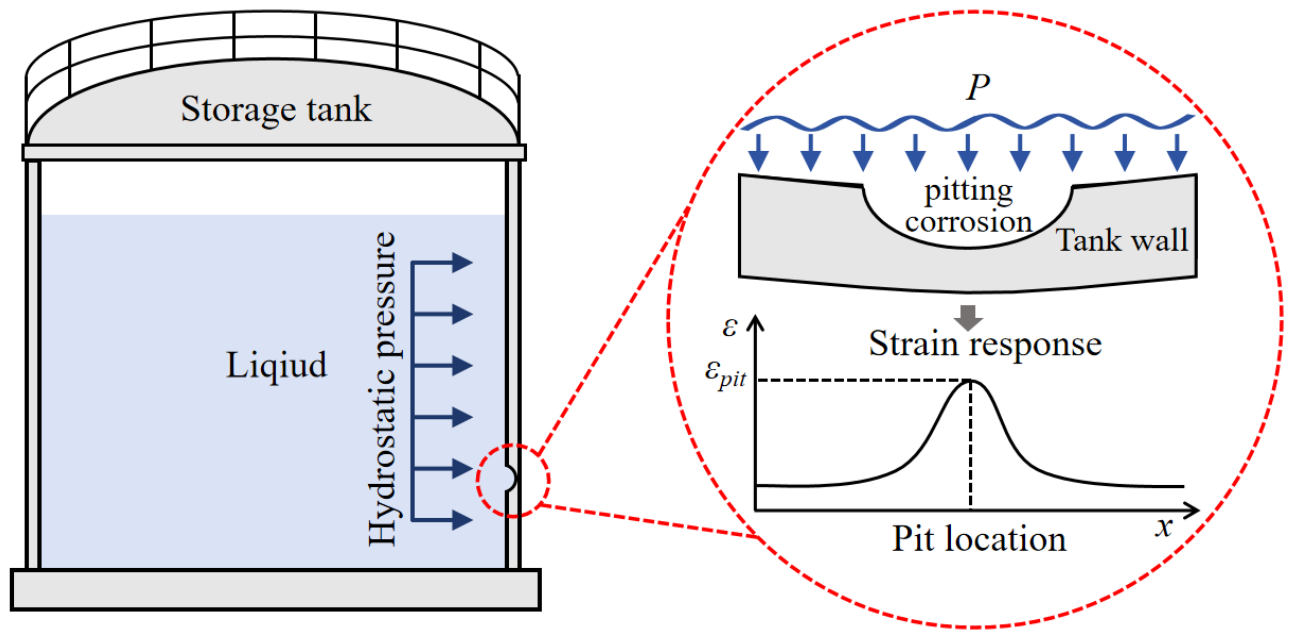
Localized corrosion decreases the remaining wall thickness and local stiffness of the tank wall. When the load is hydrostatically loaded, the redistribution of the load path around the weakened area leads to localized circumferential strain increases. Since this response is measurable on the external surface, strain changes offer a physical foundation to assess internal corrosion defects.
Figure 1 indicates that the circumferential strain response of the intact tank wall is relatively uniform under hydrostatic pressure. In the case of localized inner wall corrosion, the consequent decrease in wall thickness causes strain concentration on the external surface. The size and location of this strain response depend on the geometry of defects. Thus, circumferential strain measured externally has information about the internal corrosion state.
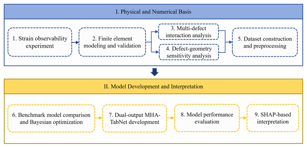
Figure 2 shows the general structure of the research. The first experiment is a partial similarity hydrostatic experiment to identify whether localized inner wall thinning generates a measurable circumferential strain response on the external surface. A parametric finite element model is then developed and assessed through mesh convergence analysis and analytical comparison. Based on this model, the interactions between the neighboring corrosion pits and the sensitivity of the strain response to the defect geometry are explored. A multi-condition finite element dataset is then created and employed to develop a data-driven model for quantitative corrosion defect inversion. Lastly, the model performance and feature contributions are compared to assess the accuracy and physical consistency of the proposed method.

2.2. Experimental Assessment of Strain Observability

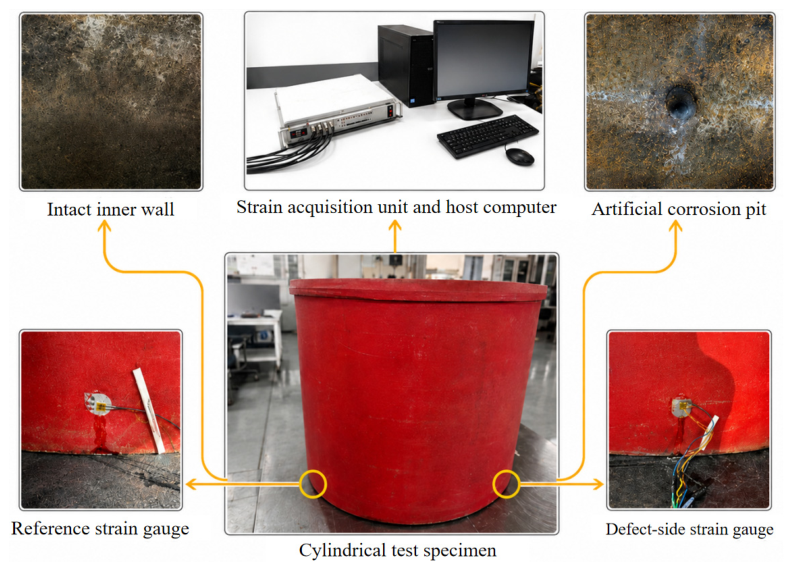
A partial similarity hydrostatic test was performed before extrapolating the conditions studied by parametric finite element simulations to establish whether localized inner wall thinning would produce a measurable strain response on the external surface. The specimen was not a strictly scaled replica of a full-scale storage tank, but it had the major physical features that controlled the response, such as a Q235 thin-walled cylindrical structure, localized thinning of the inner wall, hydrostatic loading, and external circumferential strain measurement. Thus, the strain response mechanism and external observability of corrosion was tested and not to replicate the absolute response of a full-scale tank or to directly validate the finite element model.
The height of the cylindrical specimen was 1.3 m, diameter was 1.0 m and wall thickness was 3 mm. On the inside wall of the bottom of the specimen, a circular artificial corrosion pit with a pit diameter of 10 mm and a depth of 1 mm was machined. Two three-directional strain gauges (Jiangsu Donghua Testing Technology Co., Ltd., Jingjiang, Jiangsu, China) of the same orientation were mounted on the outside surface at the same height. One of the gauges was placed directly opposite the artificial pit and the other at the diametrically opposite intact point as a reference point. The subsequent comparison was made using only the circumferential strain components.
The strain gauges were attached to DH5922N strain acquisition system (Jiangsu Donghua Testing Technology Co., Ltd., Jingjiang, Jiangsu, China), and the signals were recorded at 1 s intervals. The specimen was filled with water gradually during the test and kept in a full-water condition. The specimen was filled and allowed to stabilize after 10 min when the water level and strain readings were at equilibrium. Figure 3 illustrates the specimen, artificial pit, strain gauge system, and data acquisition system.
The two gauges were at the same elevation and thus they were subjected to the same hydrostatic head and almost similar structural and loading conditions. The main distinction between the two positions was the localized inner wall thinning under the defect-side gauge. This paired design thus allowed for the detection of the strain variation caused by the defect and reduced the impact of the overall loading conditions. The circumferential strains at the defect-side and intact reference positions were stabilized to 28 με and 8 με, respectively. The defect-side strain was about 3.5 times greater than the reference value, which indicates that localized inner wall thinning can result in a distinctly identifiable strain amplification on the outer surface. These findings justify the application of external circumferential strain as a response variable to be used in the analysis of corrosion defects later.

2.3. Finite Element Model and Assessment

2.3.1. Model Development and Mesh Independence Verification

After the experimental validation of the observability of the strain, a parametric finite element model was developed with the help of the Static Structural module of ANSYS Workbench 2023 R1. The reference structure was a typical 5000 m3 atmospheric storage tank. Other auxiliary elements, including stairways, manholes, and wind girders, were excluded since they do not have much impact on the local circumferential strain response that is being studied in this paper. The tank was thus simplified to a thin-walled cylindrical structure and modeled with 20-node SOLID186 elements. Q235 steel was modeled as a linear elastic material with an elastic modulus of 209 GPa and a Poisson’s ratio of 0.3. Its yield strength of 235 MPa was used as the reference limit for assessing the applicability of the linear elastic assumption. Table 1 presents the reference parameters used to define the finite element model.
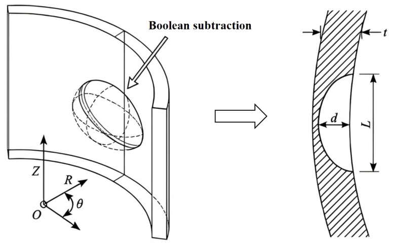
To analyze localized corrosion pits, smooth idealized geometries are often used since the depth, width, and profile of the pit directly affect the stress or strain concentration that occurs [23,24]. In this study, the localized corrosion defect was represented as an axisymmetric spherical cap pit on the inner tank wall. The cutting sphere and penetration depth were calculated at each prescribed corrosion depth d and pit diameter L, and the pit geometry was created by Boolean subtraction. In this case, d is the maximum depth of wall loss, and L denotes the pit diameter, defined as the diameter of the circular opening; therefore, it does not distinguish between the axial and circumferential directions. The defect center was adjusted at 1 m above the tank bottom, which is the lower wall area where water and impurities are likely to accumulate, and corrosion is more probable to take place. The modeling procedure and geometric definitions are presented in Figure 4.
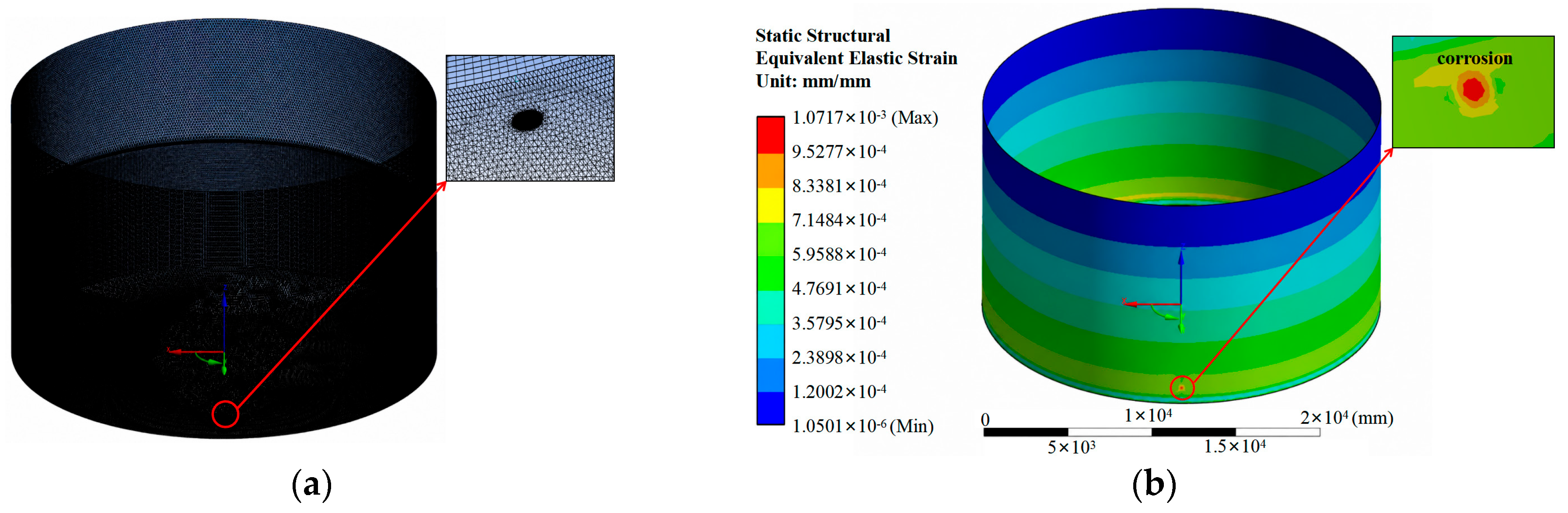
A swept mesh was used to discretize the bottom plate, while the tank wall was discretized using three-dimensional, 20-node quadratic SOLID186 elements. Local face sizing was applied to the spherical cap pit surface to resolve the steep strain gradient caused by the local reduction in wall thickness, and the transition mesh surrounding the refined region was generated automatically. The center of the bottom plate was assigned a fixed support (ux = uy = uz = 0) to eliminate rigid body motion, and the bottom support boundary was constrained in the axial direction (uz = 0). Radial and circumferential displacements were left unconstrained elsewhere. Hydrostatic pressure was applied normal to the inner surfaces of the tank wall and bottom plate and varied linearly with liquid depth, from zero at the free surface to the maximum value at the tank bottom. Figure 5a shows the global mesh and the locally refined defect region.
The strain distribution in a representative circumferential form is presented in Figure 5b. The corrosion area has a distinct localized strain increase compared to the adjacent intact wall. The highest circumferential strain in this area was obtained as the main response value to be used in the mesh convergence, mechanical response, and dataset analyses.
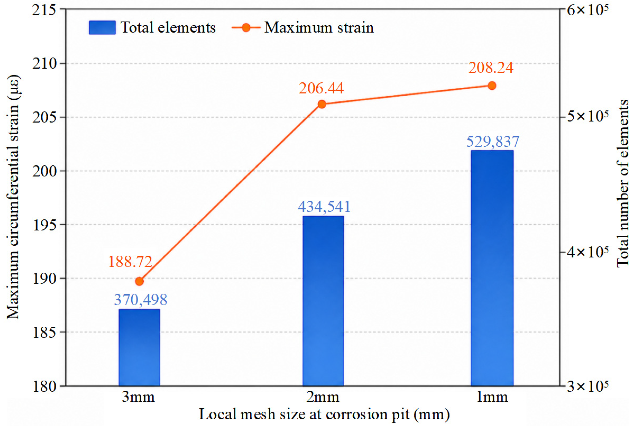
In order to assess the sensitivity of the defect region response to local mesh refinement, the corrosion pit surface was given three target element sizes of 3.0, 2.0 and 1.0 mm. The local face sizing control was the only one that was varied and the global body sizing, meshing techniques, geometry, material properties, loading conditions, and boundary constraints were kept constant. The transition elements around it were automatically regenerated in each local mesh size, which gave a total of 370,498, 434,541, and 529,837 elements, respectively. The maximum circumferential strain of each mesh configuration was obtained by the same geometrically defined corrosion region by the same result evaluation procedure.
The highest circumferential strains were recorded as 188.72, 206.44 and 208.24 με with local mesh sizes of 3.0, 2.0 and 1.0 mm, respectively, as shown in Figure 6. When the corrosion pit mesh was refined to 2.0 mm, the calculated strain was higher by 8.58%, which means that the 3.0 mm mesh was not adequate to measure the local strain concentration. Additional refinement to 2.0 to 1.0 mm only changed the calculated strain by 0.86% even though the total number of elements increased to 529,837 (434,541). This small variation shows that the response of the defect region had stabilized. Thus, a local mesh size of 2.0 mm was selected to use in further parametric simulations to obtain a compromise between numerical accuracy and computational efficiency.

2.3.2. Analytical Verification of the Global Response

Direct analytical verification of the corrosion-induced local strain field was not adopted because the three-dimensional stress and strain fields around a finite corrosion pit are complex and difficult to evaluate analytically. Instead, due to the axisymmetry of the tank geometry and hydrostatic loading, the radial displacement of the intact tank wall was evaluated using classical elastic cylindrical shell theory, which provides a well-established analytical reference for verifying the global response of the FE model [25]. Under axisymmetric small-deformation conditions, radial displacement represents the change in the tank radius and therefore directly reflects the circumferential expansion of the wall. When normalized by the tank radius, it gives the circumferential strain, εθur/R. Therefore, the radial displacement comparison is directly related to the global circumferential deformation response. Although this comparison does not directly validate the local strain at the corrosion pit, it provides a verified baseline FE model for investigating the relationship between local corrosion and strain.
Let z denote the vertical coordinate measured upward from the tank bottom and let H denote the liquid level. The hydrostatic pressure acting on the inner surface of the tank wall is expressed as
p ( z ) = ρ g ( H z )
where ρ is the liquid density and g is the gravitational acceleration. Under axisymmetric loading conditions, the radial displacement w(z) of a thin cylindrical shell satisfies
D d 4 w d z 4 + E t R 2 w = p ( z )
where E is the elastic modulus, t is the wall thickness, R is the tank radius, and D is the flexural rigidity of the cylindrical shell:
D = E t 3 12 1 v 2
where v is Poisson’s ratio. Introducing the shell characteristic parameter
λ = E t 4 R 2 D 1 / 4
The radial displacement under linearly varying hydrostatic pressure can be written as
w ( z ) = ρ g R 2 E t ( H z ) + e λ z C 1 cos ( λ z ) + C 2 sin ( λ z )
The former is the deformation of the membrane due to the hydrostatic pressure, and the latter is the local deformation due to the bottom constraint. Using the fixed bottom boundary conditions
w ( 0 ) = 0 , d w d z | z = 0 = 0
gives
C 1 = ρ g R 2 H E t , C 2 = ρ g R 2 E t 1 λ H
Substitution of Equation (7) into Equation (5) yields the radial displacement of the tank wall:
w ( z ) = ρ g R 2 E t ( H z ) e λ z H cos ( λ z ) + H 1 λ sin ( λ z )
The finite element model was used to extract radial displacements at 1, 2, 3 and 4 m tank wall heights. The relative error between the analytical and finite element results was calculated as
E r r o r = w F E w A w A × 100 %
where w A and w F E are the analytical and finite element radial displacements, respectively. The comparison is presented in Table 2.
The relative errors of the four chosen locations were between 1.15% and 5.53%, which means that there was a good agreement between the analytical and finite element results. This comparison shows that the global stiffness, distribution of hydrostatic pressure and bottom constraints were fairly modeled in the finite element model. Together with the mesh independence verification in Section 2.3.1, these results support the use of the model in the subsequent parametric analyses.

2.4. Mechanical Response and Applicability Analysis

2.4.1. Multi-Defect Interaction and Equivalent Representation

Corrosion flaws on tank walls can be in groups and not in isolated pits. Past research has demonstrated that the interaction between neighboring corrosion defects is controlled by their spacing, alignment, and relative geometry [26]. Since the following dataset and inversion model corrosion in terms of an equivalent single defect, the interaction between neighboring pits was studied to understand the relevance of this model.
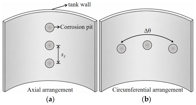
A typical case of a tank wall thickness of t = 10 mm, a corrosion depth of d = 4 mm, and a pit diameter of L = 100 mm was chosen. The same material properties, loading conditions, and boundary constraints as the finite element model described in Section 2.3 were used to establish two- and three-pit models. The pits were either in the axial or circumferential direction as illustrated in Figure 7. In the axial arrangement, the center-to-center spacing sz between neighboring pits was varied and normalized by the pit diameter L, giving the dimensionless spacing sz/L. In the circumferential arrangement, the angular separation Δθ between neighboring pits was varied. The response indicator was the maximum circumferential strain in the defect region, and the single-pit result was taken as the reference value.
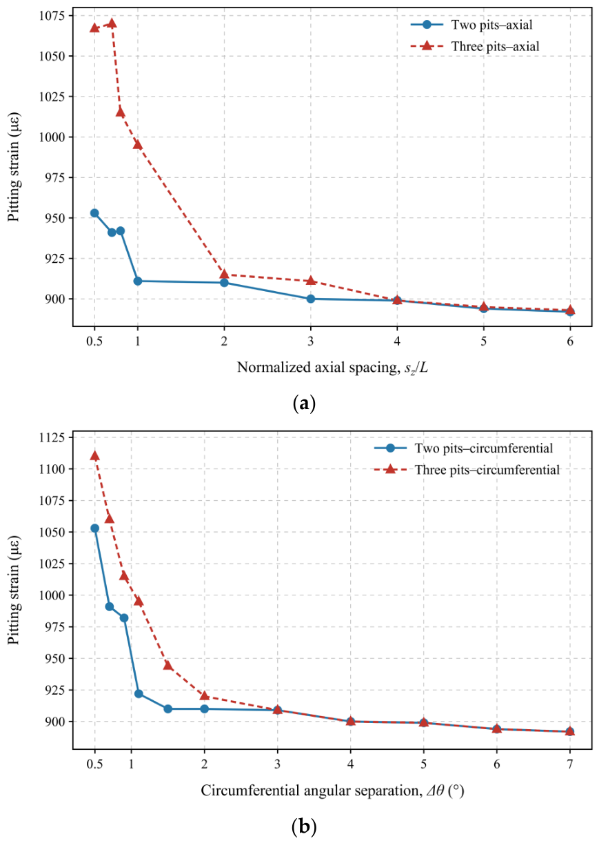
Figure 8a indicates that the maximum circumferential strain decreased with increasing normalized axial spacing sz/L. At small values of sz/L, the strain concentration regions of neighboring pits overlapped, resulting in a pronounced interaction effect. The three-pit configuration generally produced a higher strain response than the two-pit configuration. As sz/L increased, the interaction weakened, and the responses of both configurations approached the single-pit level at approximately sz/L = 2.
A similar trend was observed for the circumferential arrangement, as shown in Figure 8b. The maximum circumferential strain decreased rapidly with increasing angular separation. The interaction was stronger at small angular separations because neighboring pits collectively perturbed the circumferential load transfer path. As the angular separation increased to approximately 2°, the responses of both configurations gradually approached the single-pit level.
These findings suggest that closely spaced pits should be treated as an interacting defect group. As the spacing increases, the interaction weakens, and the pits can be represented and evaluated separately. The normalized axial spacing of approximately sz/L = 2 and the circumferential angular separation of approximately 2° apply only to the representative defect geometry and loading conditions considered in this analysis and should not be interpreted as general interaction thresholds.

2.4.2. Sensitivity of Strain Response to Defect Geometry

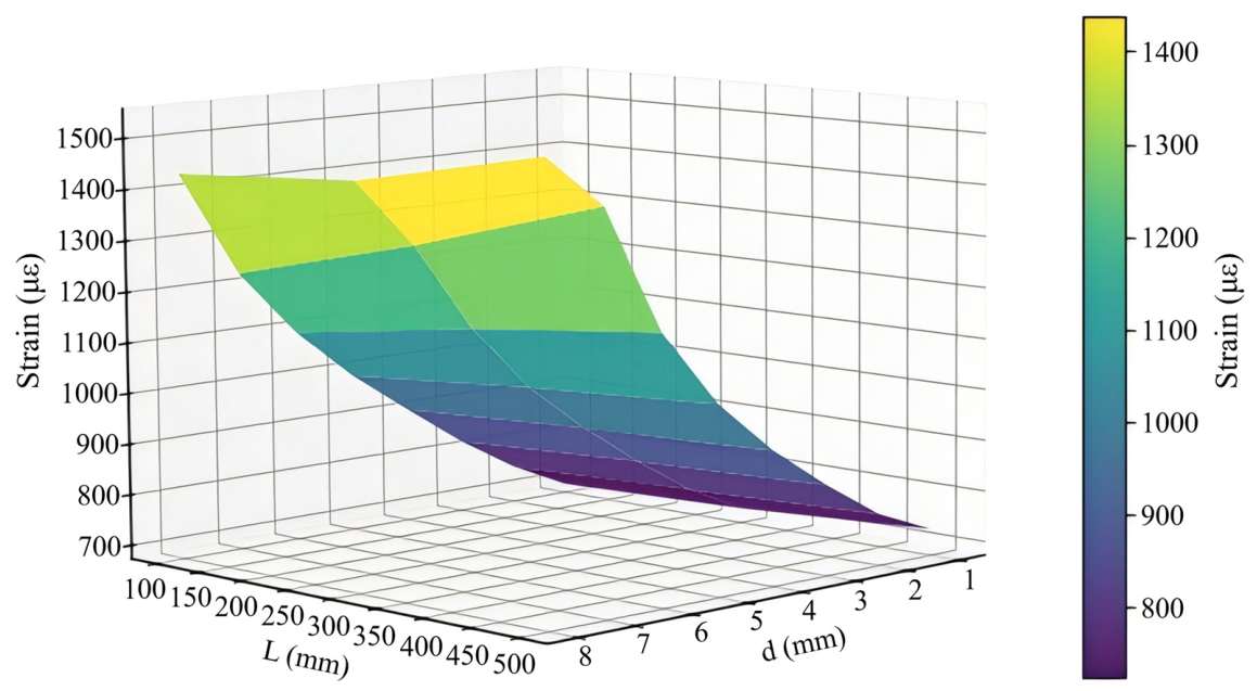
A sequence of single-pit finite element models were studied to investigate how defect geometry affects the local strain response under a representative service condition. The depth of corrosion d and the pit diameter L were varied, and the wall thickness, hydrostatic pressure, defect location, material properties, and boundary conditions were kept constant. Each combination of parameters was extracted to give the maximum circumferential strain in the corrosion region, and the response surface is shown in Figure 9.
The maximum circumferential strain was found to grow with the corrosion depth and pit diameter as indicated in Figure 9, but the sensitivities to the two parameters were not equal. The response surface rose sharply along the depth direction, which showed that the depth of corrosion was a significant factor in the local strain amplification. This effect was more pronounced when the depth was more than about 4 mm. The local stiffness was further lowered with a decrease in the remaining wall thickness, leading to a rapid rise in the maximum circumferential strain.
Pit diameter had a relatively moderate impact. At a given corrosion depth, the maximum circumferential strain increased gradually with increasing pit diameter, but the rate of increase decreased as pit diameter increased. The larger the pit diameter, the larger the region of wall-thinning, and the larger the portion of the tank wall influenced, but the smaller the incremental effect of the local peak strain.
The findings show that the main geometric parameter that determines the local strain amplification is the corrosion depth, and the secondary, but not negligible, influence is the pit diameter. In addition, the curved response surface shows that the two parameters have nonlinear and coupled effects. Different combinations of corrosion depth and pit diameter can thus produce the same local strain level, making it difficult to determine both parameters directly from a single strain value. This property of response offers the mechanical foundation of the multivariate joint inversion technique that is formulated in the next section.

3. Dataset Construction and Preprocessing

3.1. Dataset Construction

Based on the applicability analysis in Section 2.4.1, the equivalent single-defect FE model was used to generate the numerical dataset. The design space was defined in terms of wall thickness t, hydrostatic pressure p, corrosion depth d, and pit diameter L. To ensure the applicability of the linear elastic material model, additional restrictions were imposed on combinations of high hydrostatic pressure and large corrosion depth. The variables t and p were treated as predefined paired discrete variables rather than independently sampled random variables. Four pressure levels were assigned to each wall thickness: for t = 5 mm, p = 22.07, 44.14, 66.21, and 88.29 kPa; for t = 6 mm, p = 26.97, 53.95, 80.93, and 107.91 kPa; for t = 7 mm, p = 31.88, 63.76, 95.64, and 127.53 kPa; and for t = 10 mm, p = 29.70, 59.30, 89.00, and 118.70 kPa. Within each wall thickness–pressure stratum, d and L were generated using Latin hypercube sampling (LHS) [27], implemented in Python 3.9 using NumPy 2.0.2 with a fixed seed of 42. Uniform design space marginals were used within each sampling batch. The general parameter ranges were 1 ≤ d ≤ min (8, 0.8 t) mm and 50 ≤ L ≤ 500 mm. For the high-pressure cases with t = 10 mm, the upper limit of d was further restricted to 6 mm at p = 89.00 kPa and 5 mm at p = 118.70 kPa. Consequently, every case satisfied d < t, and the remaining wall thickness was at least 0.2 t, with a minimum absolute value of 1 mm.
In all simulations, the corrosion pit center was located 1 m above the tank bottom, corresponding to the corrosion-sensitive lower wall region. Thus, p represents the hydrostatic pressure at this fixed defect position, and the defect location was not treated as a variable. Parameter assignment, geometry updating, remeshing, static solution, and response extraction were automated using a Python script. A total of 1072 FE cases were generated within the restricted design space. The maximum equivalent (von Mises) stress extracted from the FE results was 212.6 MPa, which is below the yield strength of Q235 steel (235 MPa). Therefore, all cases used for model development remained within the assumed linear elastic regime.
For each simulation, the maximum circumferential strain in the corrosion region was extracted as the pitting strain εpit. The reference strain εref was obtained from an intact region at the same elevation within the same FE model. The strain concentration factor (SCF) was then calculated as
S C F = ε p i t ε r e f
The input vector of the ith sample was expressed as
x i = t i , p i , ε p i t , i , S C F i T
and the corresponding output vector was
y i = d i , L i T
The inversion framework is based on strain response features. The pitting strain provides an absolute measure of the localized circumferential response, whereas the SCF characterizes the relative strain amplification caused by localized wall thinning. Wall thickness and hydrostatic pressure describe the structural stiffness and loading conditions under which the strain response is generated, thereby helping distinguish similar strain responses produced under different conditions. The equivalent corrosion geometry is jointly characterized by corrosion depth and pit diameter, which are treated as two regression outputs.
Using a fixed random seed of 42, the 1072-case dataset was randomly divided into training and testing subsets at a ratio of 70:30, yielding 750 training cases and 322 testing cases. Model development, including hyperparameter optimization, was conducted exclusively using the training subset, while the held-out testing subset was used only for final performance evaluation. Both subsets were derived from the same FE formulation, spherical cap defect representation, linear elastic material model, fixed defect location, and restricted elastic design space. Therefore, the reported testing results quantify the interpolation performance for previously unseen parameter combinations within the FE-generated design space rather than external validation using a different numerical model, defect geometry, tank, or experimental dataset.

3.2. Data Analysis and Preprocessing

The descriptive statistics of the four input variables and two output variables are summarized in Table 3. The variables had significant differences in their units and numerical ranges. Specifically, the range of numbers of the pit diameter was significantly broader than the corrosion depth, whereas the maximum circumferential strain was many orders of magnitude lower than the structural and loading parameters. These variations were taken into account in the following data preprocessing.
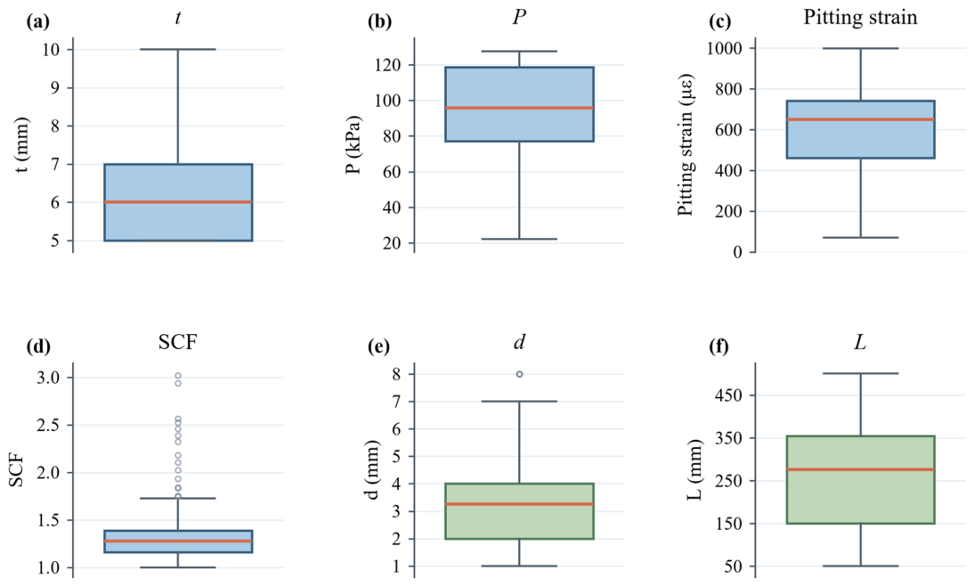
As shown in Figure 10, most variables exhibit relatively compact distributions. Although several high-value cases in the SCF and corrosion depth distributions lie beyond the box plot whiskers, these cases remain within the predefined parameter ranges and satisfy the elastic criterion described in Section 3.1.
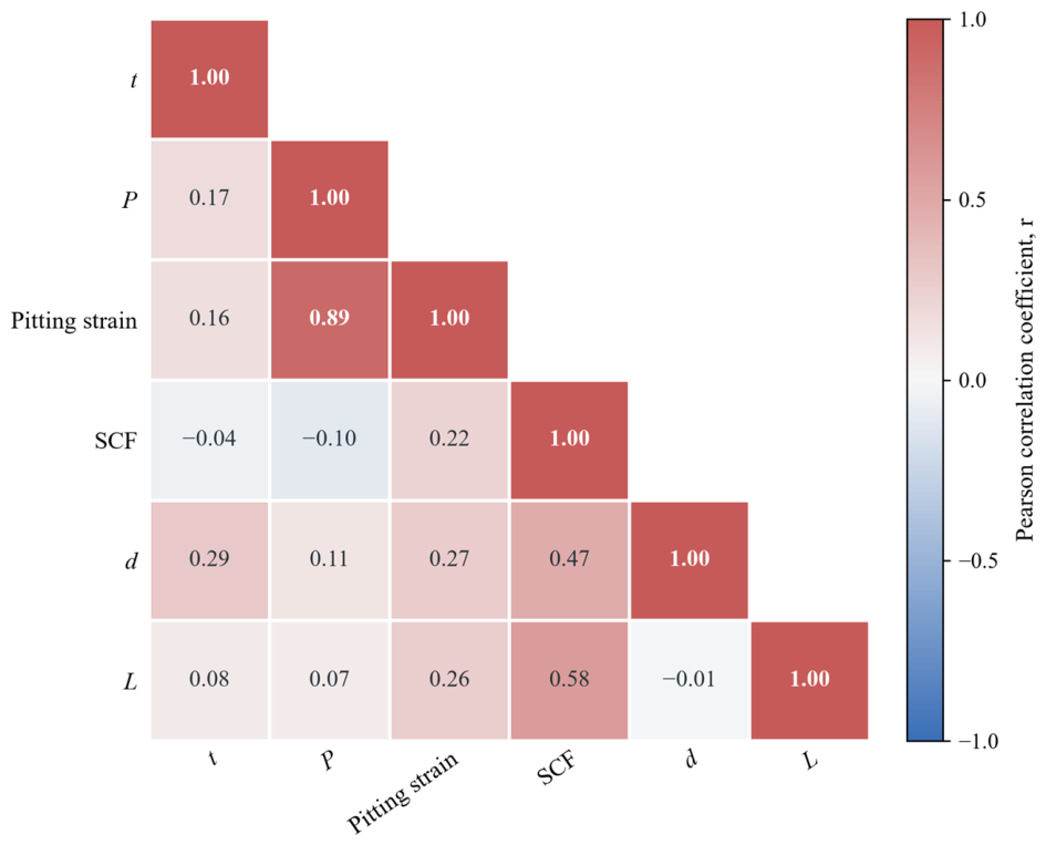
The pairwise linear relationships among the variables were evaluated using Pearson correlation analysis. As shown in Figure 11, hydrostatic pressure and maximum circumferential strain were strongly positively correlated (r = 0.89), consistent with the increase in strain response with applied loading in the elastic regime. The absolute values of all other pairwise correlations did not exceed 0.58. Corrosion depth was positively correlated with maximum circumferential strain (r = 0.27) and SCF (r = 0.47), while pit diameter showed corresponding correlations of 0.26 and 0.58. These weak-to-moderate correlations indicate that the relationship between either defect parameter and any individual input feature is not adequately described by a simple linear mapping. Therefore, the correlation matrix was used to characterize the relationships among variables rather than as a direct feature elimination criterion.
Intelligent frameworks that are based on feature selection have been used to predict corrosion defects to determine informative input variables. All four input variables were not dropped in the current study since they are unique structural, loading, and strain response properties. Further analysis was done on variance inflation factor (VIF) to determine multicollinearity of the four input variables [28]:
V I F j = 1 1 R j 2
where R j 2 is the coefficient of determination of the regression of the jth input feature on the other input features. The VIF values of wall thickness, hydrostatic pressure, maximum circumferential strain, and SCF were 1.03, 8.95, 9.31, and 1.90, respectively. All values were below the practical screening threshold of 10, although hydrostatic pressure and maximum circumferential strain showed relatively high VIF values. This threshold was treated as a diagnostic rather than an automatic feature removal rule. Both variables were retained because hydrostatic pressure represents the applied load, whereas maximum circumferential strain represents the corresponding structural response. SCF was also retained because it characterizes localized strain amplification relative to the reference region.
The four input features were standardized with the following equation to remove the differences in numerical scale.
x * = x μ σ
where x and x * denote the original and standardized values, respectively, and μ and σ are the mean and standard deviation calculated from the training set. The same parameters were then applied to the testing set to prevent information leakage.
The two output variables were processed separately. The depth of corrosion was directly standardized by means of the Equation (14). Since the numerical range of pit diameter was significantly greater, it was initially transformed with
L l o g = ln L
The values were then transformed and standardized. The two outputs were then transformed back to their original scales, and the performance measures were then calculated after prediction. This process minimized the scale differences between the two targets and retained the dual-output formulation of the inversion task.

4. Development and Evaluation of the Corrosion Defect Inversion Model

4.1. Benchmark Model Comparison and Selection

Five standard regression algorithms were chosen as benchmark algorithms: random forest (RF), support vector regression (SVR), XGBoost, multilayer perceptron (MLP), and TabNet. These models are various learning processes, such as bagging-based decision trees, kernel-based regression, boosting-based decision trees, traditional neural networks, and attention-based learning with structured tabular data. Their performance was contrasted to determine an appropriate backbone model to learn the nonlinear relationship between external strain responses and corrosion defect geometry.
The same dataset, training–testing partition, and preprocessing procedure as in Section 3 were used to evaluate all benchmark models. The input variables were tank wall thickness, hydrostatic pressure, maximum circumferential strain, and strain concentration factor, and corrosion depth and pit diameter were considered the two target variables. Each of the methods was tested within the same two-target regression framework. The preprocessing parameters were only obtained using the training set and then applied to the testing set to avoid information leakage.
Since the predictive performance of each model depends on its hyperparameter configuration, BO was applied consistently to all five benchmark models. BO builds a surrogate model of the validation objective and applies an acquisition function to identify promising hyperparameter combinations, making it suitable for computationally expensive black box optimization [29]. For each model, BO was conducted for 50 iterations using five-fold cross-validation on the training subset. After BO, each model was refitted using the complete training subset with the selected hyperparameters and evaluated once on the held-out testing subset. The Expected Improvement acquisition function was used to select the hyperparameter combination evaluated at each iteration. The optimization objective was to minimize the mean cross-validation root mean square error (RMSE) averaged across the standardized corrosion depth output d and the log-transformed and standardized pit diameter output L. The hyperparameter combination with the lowest objective value was selected. The testing subset was excluded from hyperparameter optimization and was used only for the final performance evaluation. Table 4 summarizes the hyperparameter search spaces and the values selected by BO.
The mean absolute error (MAE), RMSE, and coefficient of determination (R2) were used to assess the optimized models. MAE explains the mean size of the prediction errors, and RMSE gives more weight to the large errors. Lower MAE and RMSE values indicate better prediction accuracy. R2 value explains the relationship between the predicted and actual values with a value nearer to 1 showing better performance of the model. The three measures were computed individually on the corrosion depth and pit diameter once the predicted measures were transformed back to their physical units. The testing performance of the five optimized benchmark models is summarized in Table 5.
TabNet was the best overall predictor in the conditions studied, with the lowest MAE and RMSE values and the highest R2 values of corrosion depth and pit diameter. Thus, TabNet was chosen as the most appropriate model to be used in the current corrosion defect inversion task.

4.2. Development and Evaluation of the Dual-Output MHA-TabNet Model

According to the benchmark comparison in Section 4.1, BO-TabNet was chosen as the backbone model to be developed. TabNet is a deep learning model that works with structured tabular data. Recent reviews and enhanced TabNet variants have demonstrated that nonlinear representation learning can be achieved by sequential attention and step-wise feature selection, and still maintain some level of interpretability [30,31]. An Attentive Transformer is used at every decision step to produce a sparse feature mask to choose the variables that are important to the decision at hand, and a Feature Transformer transforms the chosen variables into higher-order representations.
Even though TabNet is capable of dynamically choosing influential features, its Feature Transformer primarily uses fully connected layers and nonlinear activation functions. The sparse mask selects the variables to be kept at each decision step but is not very effective in explicitly modeling joint interactions between tank wall thickness, hydrostatic pressure, maximum circumferential strain, and SCF. This constraint can limit the modeling of the highly coupled nonlinear interaction between strain responses and corrosion geometry.
The feature-interaction methods that rely on attention to tabular data have shown that multiple heads can learn complementary relationships between variables and informative feature weighting [32]. To enhance cross-feature interactions, MHA modules were introduced into the TabNet architecture. Scaled dot-product attention is defined as
A t t e n t i o n ( Q , K , V ) = s o f t m a x Q K T d k V
where Q , K , and V are the query, key, and value matrices, respectively, and d k is the dimension of the key vectors.
The scaling term restricts overly large dot-product values and enhances the numerical stability of the Softmax operation.
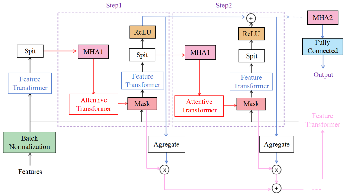
For a mini-batch containing B samples, the standardized input tensor has a shape of B × 4, with the four columns corresponding to tank wall thickness, hydrostatic pressure, maximum circumferential strain, and SCF. At each decision step, the output of the Feature Transformer is divided by the Split operation into a decision representation and an attention representation, with dimensions of B × na and B × na, respectively. As illustrated in Figure 12, MHA1 is applied to the attention branch between the Split operation and the Attentive Transformer. The attention representation is converted into four ordered feature-associated tokens through feature-specific linear projections, with each token corresponding to one input variable. Using the fixed embedding dimension of 64, the resulting MHA1 input tensor has a shape of B × 4 × 64. With the two attention heads selected by BO, each head has an embedding dimension of 32. After head separation, the query, key, and value tensors each have a shape of B × 2 × 4 × 32. The outputs of the attention heads are concatenated and linearly transformed as
M H A ( X ) = C o n c a t h e a d 1 , , h e a d h W o , h e a d i = A t t e n t i o n X W i Q , X W i K , X W i V
In Equation (17), X denotes the token tensor supplied to the corresponding MHA module. Equation (17) is applied separately to MHA1 and MHA2, and the two modules do not share weights. For MHA1, the multi-head output retains a shape of B × 4 × 64 and is subsequently projected back to a representation with a shape of B × na. The resulting representation is passed to the Attentive Transformer to generate the sparse feature mask for the next decision step. At the global level, the decision representations produced by the four decision steps are treated as four ordered step-wise tokens. Each decision representation, with a shape of B × na, is projected to 64 dimensions, resulting in an MHA2 input tensor with a shape of B × 4 × 64. With two attention heads, the corresponding query, key, and value tensors each have a shape of B × 2 × 4 × 32. MHA2 captures the dependencies among the decision-step representations. Its output is summed across the four step-wise tokens and passed to a fully connected regression layer with two output nodes:
y ^ = d ^ , L ^ T
where d ^ and L ^ denote the predicted corrosion depth and pit diameter, respectively. The two output nodes share the fused representation produced by MHA2, allowing for the model to learn information common to both targets while retaining target-specific predictions [33]. Consequently, corrosion depth and pit diameter are predicted simultaneously by a single shared model rather than by two independently trained neural networks.
The BO procedure outlined in Section 4.1 was used to determine the hyperparameters of MHA-TabNet. Since the modified architecture added attention-specific parameters, the search space had the number of attention heads and the attention dropout rate besides the original TabNet parameters. The hyperparameter search spaces and the values selected through BO are listed in Table 6. The optimized model is henceforth called BO-MHA-TabNet.
To compare the baseline and modified architectures under the same model development procedure, the BO-TabNet model selected in Section 4.1 was compared with BO-MHA-TabNet. The training and testing samples, preprocessing procedure, BO strategy, and evaluation metrics were the same in all models. Their results on the same held-out testing set are summarized in Table 7.
Table 7 indicates that BO-MHA-TabNet performed better than BO-TabNet in the inversion of corrosion depth and pit diameter. For corrosion depth, the testing MAE and RMSE decreased from 0.248 and 0.354 mm to 0.226 and 0.257 mm, respectively, while R2 increased from 0.9263 to 0.9612. For pit diameter, the MAE decreased from 28.336 to 24.252 mm, the RMSE decreased from 41.612 to 32.505 mm, and R2 increased from 0.8979 to 0.9377.
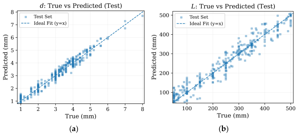
The regression fitting results of BO-MHA-TabNet on the testing set are shown in Figure 13. The actual and predicted values are represented by the horizontal and vertical coordinates, respectively, and the ideal prediction is represented by the dashed y = x line. The predictions of corrosion depth are closely distributed around the ideal line. The predictions of pit diameter also show good overall agreement with the actual values, although a relatively broader and more scattered distribution is observed compared with corrosion depth, with no evident systematic deviation over the investigated range.
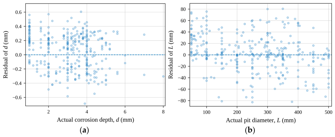
Figure 14 shows the prediction residuals with respect to the actual corrosion depth and pit diameter. The residuals of corrosion depth are mainly distributed around zero and remain relatively stable over the investigated range. For pit diameter, the residuals are also distributed around zero, with a somewhat wider dispersion than that of corrosion depth but without an evident increase with diameter. As shown in Table 8, the absolute prediction errors of both outputs remain generally stable across the different value intervals, whereas the normalized errors are more pronounced for smaller defects. Here, normalized mean absolute error (NMAE) is calculated as the interval MAE divided by the mean actual value within the corresponding interval. The NMAE reaches 13.79% for corrosion depths of 1–3 mm and 23.86% for pit diameters of 50–200 mm but decreases to 4.09% and 6.27% in the largest depth and diameter intervals, respectively. These results indicate that the global average metrics should be interpreted together with the actual defect dimensions, particularly for smaller defects.
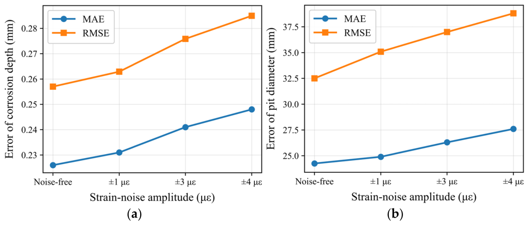
To evaluate the influence of strain measurement uncertainty on the inversion results, bounded random noise was independently introduced into εpit and εref in the testing set. Given the approximate ±1 με strain measurement accuracy of the DH5922N-based acquisition system, disturbance levels of ±1, ±3, and ±4 με were selected to represent nominal, clearly amplified, and conservative upper measurement uncertainties, respectively. For each noise level, the perturbations were sampled uniformly within the corresponding bounds. The strain concentration factor was then recalculated as SCF = εpit/εref, and the perturbed strain features were evaluated using the trained BO-MHA-TabNet model without retraining. Each noise condition was repeated 50 times, and the mean prediction metrics were reported.
As shown in Figure 15, the prediction performance gradually decreased with increasing strain noise amplitude. For corrosion depth, the MAE increased from 0.226 to 0.231, 0.241, and 0.248 mm, while the RMSE increased from 0.257 to 0.263, 0.276, and 0.285 mm, and R2 decreased from 0.9612 to 0.9594, 0.9553, and 0.9523. For pit diameter, the MAE increased from 24.252 to 24.900, 26.300, and 27.600 mm, while the RMSE increased from 32.505 to 35.089, 36.995, and 38.807 mm, and R2 decreased from 0.9377 to 0.9274, 0.9193, and 0.9112. These results indicate that measurement uncertainty gradually reduces prediction accuracy, although the model retains its overall predictive capability within the investigated noise range.
Because BO-TabNet and BO-MHA-TabNet used the same data partition, preprocessing procedure, BO strategy, and evaluation metrics, their testing results can be compared directly. As shown in Table 7, BO-MHA-TabNet achieved lower MAE and RMSE values and higher R2 values for both corrosion depth and pit diameter. Although the magnitude of improvement varied between the two targets and across the three metrics, the optimized BO-MHA-TabNet configuration achieved better overall testing performance than BO-TabNet under the present conditions. BO-MHA-TabNet was therefore adopted as the final dual-output corrosion defect inversion model.

4.3. SHAP-Based Interpretation

Although BO-MHA-TabNet achieved high prediction accuracy, its nonlinear internal structure makes it difficult to determine how input variables contribute to the inversion results. The final BO-MHA-TabNet model was thus subjected to SHAP to measure the contribution of each input feature [34,35]. SHAP analysis was performed separately for the two model outputs. A positive SHAP value means that the respective feature enhances the predicted corrosion depth or pit diameter compared to the baseline prediction, and a negative value means that it reduces the contribution.
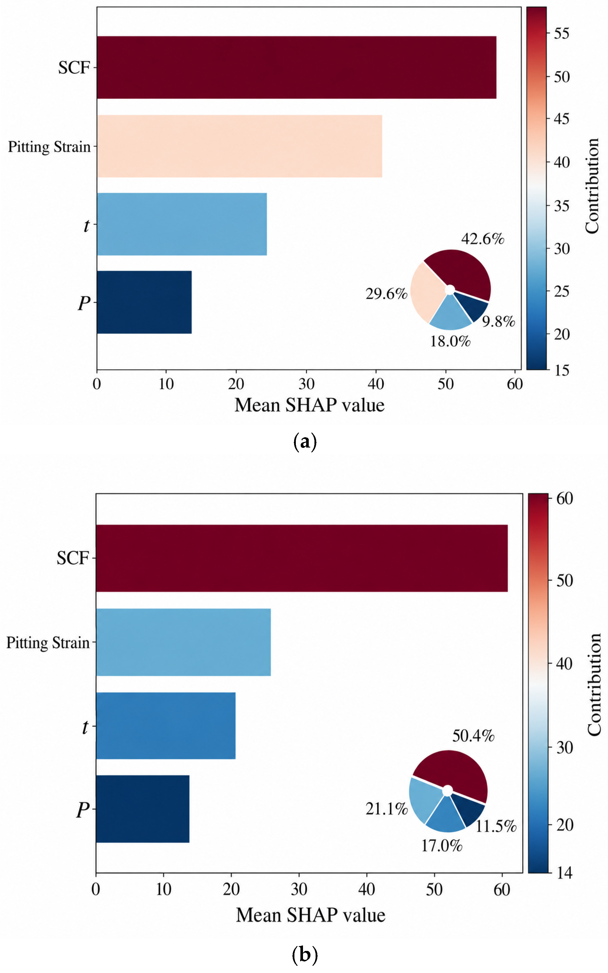
The mean absolute SHAP value was used to assess the global significance of each feature. The feature rankings for the inversion of corrosion depth and pit diameter were generally similar, as indicated in Figure 16. The most significant feature was the strain concentration factor, which contributed about 42–43% of the total contribution to prediction of corrosion depth and about 50% of the contribution to prediction of pit diameter. The highest circumferential strain was second, with a contribution of about 29–30% and 21–22% to the two outputs, respectively. In comparison, tank wall thickness added about 17–18%, and hydrostatic pressure added about 9–12%.
The prevalence of the two strain response characteristics is in line with the physical nature of the proposed inversion method. The strain concentration factor is the amplification of the local response compared to an intact region at the same elevation. Localized thinning of the wall disrupts the circumferential load transfer path and enhances deformation around the corrosion pit, rendering SCF sensitive to defect geometry variations. The maximum circumferential strain is the absolute measure of local deformation and is a direct measure of the decrease in local stiffness. The structural and loading context is given by tank wall thickness and hydrostatic pressure, but some of their effect is already represented by the two strain response features. Their SHAP contributions are thus smaller yet still needed to differentiate similar strain responses produced under varying structural and loading conditions.
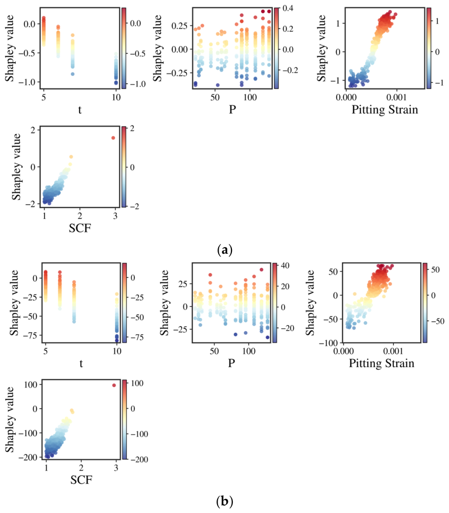
The nonlinear dependence of the four inputs is also demonstrated by the SHAP dependence plots in Figure 17. The points are one sample each, and the horizontal axis is the value of the feature, and the vertical axis is the SHAP contribution. With the increase of SCF, between about 1 and 3, the SHAP value of both outputs gradually shifted to positive. This indicates that stronger local strain concentration led the model to predict larger corrosion depth and pit diameter. The maximum circumferential strain also showed a similar increasing trend with higher strain values tending to contribute positively to both inversion results. The SHAP trends are consistent with the mechanical trends observed in the FE sensitivity analysis.
The thickness of tank walls showed a general negative SHAP trend in the data set under study, which means that it was primarily a structural stiffness variable in the model decision process. Hydrostatic pressure had a smaller SHAP range than the two strain response features. Its primary role was to characterize the overall loading level, whereas local amplification caused by defects was better characterized by the maximum circumferential strain and SCF.
In general, the SHAP results indicate that BO-MHA-TabNet mainly uses local strain amplification due to corrosion to predict defect geometry, and tank wall thickness and hydrostatic pressure are complementary structural and loading data. The rankings of feature importance and dependence trends are in line with the local stiffness reduction and strain concentration mechanisms developed in Section 2. This uniformity enhances the physical plausibility and transparency of the strain-based corrosion defect inversion model. SHAP explains the associations that the model has learned but does not give independent causal evidence; it is used here to ensure that the model decision patterns are consistent with the observed mechanical response.


5. Conclusions and Discussion

This study develops a strain-based approach to quantitatively estimate localized corrosion defects in the walls of storage tanks. The main conclusions are summarized as follows.
  • The partial similarity hydrostatic test confirmed that localized inner wall thinning generates measurable circumferential strain amplification on the outer surface, supporting strain-based corrosion inversion.
  • Corrosion depth and pit diameter have nonlinear, coupled effects on the strain response, with corrosion depth exerting the stronger influence. A single strain value is therefore insufficient to determine both parameters.
  • On the held-out testing subset of the FE-generated dataset, BO-MHA-TabNet predicted corrosion depth and pit diameter with MAEs of 0.226 and 24.252 mm, respectively. The corresponding R2 values were 0.9612 and 0.9377, indicating improved performance over BO-TabNet. The reported performance improvement of BO-MHA-TabNet over BO-TabNet is based on a single fixed data partition, and the corresponding metrics represent interpolation performance within the FE-generated design space rather than experimentally demonstrated defect sizing accuracy.
  • SHAP analysis identified the strain concentration factor and maximum circumferential strain as the most significant features, consistent with local stiffness reduction and strain concentration. Tank wall thickness and hydrostatic pressure provided complementary information on stiffness and loading.
The inferences are dependent on the parameter ranges and modeling assumptions under investigation. The localized corrosion was modeled by an equivalent spherical cap pit in a predefined monitoring area, and the current model is aimed at estimating corrosion depth and pit diameter. Moreover, ideal finite element fields were used to extract the maximum circumferential strain and strain concentration factor. Thus, the accuracy reported is the inversion capability under controlled strain feature conditions and not the overall performance of a field monitoring system.
Overall, the results demonstrate the feasibility of numerically relating externally observable circumferential strain features to localized corrosion geometry. The proposed framework is currently intended for assisted defect sizing after a potentially corroded region has been identified using an existing inspection method. External circumferential-strain sensors would then be arranged over and around the candidate region to obtain the maximum local strain, while reference strain would be measured at intact locations at the same elevation; wall thickness and hydrostatic pressure would be obtained from structural records and liquid-level information, respectively. For future standalone monitoring, densely distributed sensor arrays, such as fiber Bragg grating arrays, could first localize abnormal strain regions and then provide the strain features required for inversion. Such implementation requires further investigation of sensor spacing, strain peak offset, local welds, geometric imperfections, sensor bonding, and possible corrosion in the reference region. Experimental validation of quantitative defect reconstruction under these practical conditions and irregular corrosion morphologies is still required.

Author Contributions

Conceptualization, L.Z., J.S. and Z.W.; methodology, L.Z.; software, L.Z.; validation, L.Z., X.S. and L.C.; formal analysis, L.Z.; investigation, L.Z., X.S. and L.C.; resources, J.S. and Z.W.; data curation, L.Z.; writing—original draft preparation, L.Z.; writing—review and editing, J.S., X.S. and Z.W.; visualization, L.Z.; supervision, J.S. and Z.W.; project administration, J.S. and Z.W.; funding acquisition, J.S. and Z.W. All authors have read and agreed to the published version of the manuscript.

Funding

This research was funded by the Science and Technology Project of China Huanqiu Contracting & Engineering Co., Ltd., grant number 2246E-CA-MC-002.

Institutional Review Board Statement

Not applicable.

Informed Consent Statement

Not applicable.

Data Availability Statement

The original contributions presented in this study are included in the article. Further inquiries can be directed to the corresponding authors.

Conflicts of Interest

The authors declare that this study received funding from China Huanqiu Contracting & Engineering Co., Ltd. The funder had the following involvement with the study: study design, analysis, and interpretation of data.

References

  1. Qi, S.; Shuai, J.; Shi, L.; Li, Y.; Zhou, L. Quantitative risk assessment of leakage accident of crude oil storage tank based on fuzzy Bayesian network and improved AHP. J. Loss Prev. Process Ind. 2024, 90, 105341. [Google Scholar] [CrossRef] [Scilit]
  2. Dominici, L.E.; Del Panno, M.T.; Viera, M.R. Effect of tetrakis(hydroxymethyl)phosphonium sulfate (THPS) on the microbial community and corrosion of carbon steel in a simulated crude-oil storage tank environment. Geoenergy Sci. Eng. 2024, 236, 212775. [Google Scholar] [CrossRef] [Scilit]
  3. He, L.; Wu, J.; Wang, X.; Kang, Y.; Huang, Z.; Wang, H.; Wang, W. Safety assessment of vertical storage tank based on robot ultrasonic online inspection. J. Nondestruct. Eval. 2023, 42, 10. [Google Scholar] [CrossRef] [Scilit]
  4. Zhang, Y.; Wang, S.; Liu, J.; Liu, D.; Li, T.; Wu, W. A corrosion assessment methodology based on triangular intuitionistic fuzzy comprehensive evaluation (TIFCE) with analytic network process (TIFANP): An application to external corrosion of the storage tank floor. Expert Syst. Appl. 2024, 238, 121896. [Google Scholar] [CrossRef] [Scilit]
  5. Liu, Y.; Tan, X.; Bao, Y. Machine learning-assisted intelligent interpretation of distributed fiber optic sensor data for automated monitoring of pipeline corrosion. Measurement 2024, 226, 114190. [Google Scholar] [CrossRef] [Scilit]
  6. Liu, Y.; Huang, Y.; Bao, Y. Machine learning-empowered automatic analysis of distributed fiber optic sensor data for monitoring coincident corrosion and cracks in pipelines. Measurement 2025, 247, 116805. [Google Scholar] [CrossRef] [Scilit]
  7. Chen, Y.; Tian, Z.; Wei, H.; Dong, S. Reliability analysis of corroded pipes using MFL signals and residual neural networks. Process Saf. Environ. Prot. 2024, 184, 1131–1142. [Google Scholar] [CrossRef] [Scilit]
  8. Pan, J.; Gao, L. A novel method for defects marking and classifying in MFL inspection of pipeline. Int. J. Press. Vessels Pip. 2023, 202, 104892. [Google Scholar] [CrossRef] [Scilit]
  9. Zhou, R.; Gu, X.; Luo, X. Residual strength prediction of X80 steel pipelines containing group corrosion defects. Ocean Eng. 2023, 274, 114077. [Google Scholar] [CrossRef] [Scilit]
  10. Chen, Y.; Hou, F.; Dong, S.; Guo, L.; Xia, T.; He, G. Reliability evaluation of corroded pipeline under combined loadings based on back propagation neural network method. Ocean Eng. 2022, 262, 111910. [Google Scholar] [CrossRef] [Scilit]
  11. Li, X.; Jia, R.; Zhang, R. A data-driven methodology for predicting residual strength of subsea pipeline with double corrosion defects. Ocean Eng. 2023, 279, 114530. [Google Scholar] [CrossRef] [Scilit]
  12. Chen, Z.; Li, X.; Wang, W.; Li, Y.; Shi, L.; Li, Y. Residual strength prediction of corroded pipelines using multilayer perceptron and modified feedforward neural network. Reliab. Eng. Syst. Saf. 2023, 231, 108980. [Google Scholar] [CrossRef] [Scilit]
  13. Pereira, A.A.; Neves, A.C.; Ladeira, D.; Caprace, J.-D. Corrosion prediction of FPSOs hull using machine learning. Mar. Struct. 2024, 97, 103652. [Google Scholar] [CrossRef] [Scilit]
  14. Lu, H.; Peng, H.; Xu, Z.-D.; Matthews, J.C.; Wang, N.; Iseley, T. A feature selection–based intelligent framework for predicting maximum depth of corroded pipeline defects. J. Perform. Constr. Facil. 2022, 36, 04022044. [Google Scholar] [CrossRef] [Scilit]
  15. Ben Seghier, M.E.A.; Höche, D.; Zheludkevich, M. Prediction of the internal corrosion rate for oil and gas pipeline: Implementation of ensemble learning techniques. J. Nat. Gas Sci. Eng. 2022, 99, 104425. [Google Scholar] [CrossRef] [Scilit]
  16. Song, Y.; Wang, Q.; Zhang, X.; Dong, L.; Bai, S.; Zeng, D.; Zhang, Z.; Zhang, H.; Xi, Y. Interpretable machine learning for maximum corrosion depth and influence factor analysis. npj Mater. Degrad. 2023, 7, 9. [Google Scholar] [CrossRef] [Scilit]
  17. Li, X.; Jia, R.; Zhang, R.; Yang, S.; Chen, G. A KPCA-BRANN based data-driven approach to model corrosion degradation of subsea oil pipelines. Reliab. Eng. Syst. Saf. 2022, 219, 108231. [Google Scholar] [CrossRef] [Scilit]
  18. Akhlaghi, B.; Mesghali, H.; Ehteshami, M.; Mohammadpour, J.; Salehi, F.; Abbassi, R. Predictive deep learning for pitting corrosion modeling in buried transmission pipelines. Process Saf. Environ. Prot. 2023, 174, 320–327. [Google Scholar] [CrossRef] [Scilit]
  19. Guang, Y.; Wang, W.; Song, H.; Mi, H.; Tang, J.; Zhao, Z. Prediction of external corrosion rate for buried oil and gas pipelines: A novel deep learning method with DNN and attention mechanism. Int. J. Press. Vessels Pip. 2024, 209, 105218. [Google Scholar] [CrossRef] [Scilit]
  20. Hu, J. Prediction of the internal corrosion rate for oil and gas pipelines and influence factor analysis with interpretable ensemble learning. Int. J. Press. Vessels Pip. 2024, 212, 105329. [Google Scholar] [CrossRef] [Scilit]
  21. Tan, L.; Yang, Y.; Zhang, K.; Liao, K.; He, G.; Tian, J.; Lu, X. Prediction of internal corrosion rate for gas pipeline: A new method based on transformer architecture. Comput. Chem. Eng. 2025, 198, 109084. [Google Scholar] [CrossRef] [Scilit]
  22. Sun, S.; Cui, Z.; Zhang, D. Machine learning-based maximum pipeline pitting corrosion depth prediction using hybrid FVIM-BNN-XGB model. Eng. Fail. Anal. 2025, 175, 109603. [Google Scholar] [CrossRef] [Scilit]
  23. Shojai, M.S.; Schaumann, P.; Brömer, T. Probabilistic modelling of pitting corrosion and its impact on stress concentrations in steel structures in the offshore wind energy. Mar. Struct. 2022, 84, 103232. [Google Scholar] [CrossRef] [Scilit]
  24. Zeng, S.; Ren, S.; Gu, S.; Gu, Y.; Kong, C.; Zhou, Q. Effects of size parameters of stepwise corrosion pit on stress concentration of steel and its computation model establishment. KSCE J. Civ. Eng. 2022, 26, 2813–2825. [Google Scholar] [CrossRef] [Scilit]
  25. Zhao, M. A novel elastic analytical model for API 650 liquid storage tanks: Stress and deformation analysis under hydrostatic loads. J. Press. Vessel Technol. 2026, 1–24. [Google Scholar] [CrossRef] [Scilit]
  26. Zhang, Y.; Wang, W.; Shuai, J.; Shuai, Y.; Hua, L.; Lv, Z. A novel assessment method to identifying the interaction between adjacent corrosion defects and its effect on the burst capacity of pipelines. Ocean Eng. 2023, 281, 114842. [Google Scholar] [CrossRef] [Scilit]
  27. McKay, M.D.; Beckman, R.J.; Conover, W.J. A comparison of three methods for selecting values of input variables in the analysis of output from a computer code. Technometrics 1979, 21, 239–245. [Google Scholar] [CrossRef] [Scilit]
  28. O’Brien, R.M. A caution regarding rules of thumb for variance inflation factors. Qual. Quant. 2007, 41, 673–690. [Google Scholar] [CrossRef] [Scilit]
  29. Shahriari, B.; Swersky, K.; Wang, Z.; Adams, R.P.; de Freitas, N. Taking the human out of the loop: A review of Bayesian optimization. Proc. IEEE 2016, 104, 148–175. [Google Scholar] [CrossRef] [Scilit]
  30. Borisov, V.; Leemann, T.; Seßler, K.; Haug, J.; Pawelczyk, M.; Kasneci, G. Deep neural networks and tabular data: A survey. IEEE Trans. Neural Netw. Learn. Syst. 2024, 35, 7499–7519. [Google Scholar] [CrossRef] [Scilit] [PubMed]
  31. Liu, J.; Tian, T.; Liu, Y.; Hu, S.; Li, M. iTabNet: An improved neural network for tabular data and its application to predict socioeconomic and environmental attributes. Neural Comput. Appl. 2023, 35, 11389–11402. [Google Scholar] [CrossRef] [Scilit]
  32. Pham, H.; Tan, Y.; Singh, T.; Pavlopoulos, V.; Patnayakuni, R. A multi-head attention-like feature selection approach for tabular data. Knowl.-Based Syst. 2024, 301, 112250. [Google Scholar] [CrossRef] [Scilit]
  33. Borchani, H.; Varando, G.; Bielza, C.; Larrañaga, P. A survey on multi-output regression. WIREs Data Min. Knowl. Discov. 2015, 5, 216–233. [Google Scholar] [CrossRef] [Scilit]
  34. Lundberg, S.M.; Erion, G.; Chen, H.; DeGrave, A.; Prutkin, J.M.; Nair, B.; Katz, R.; Himmelfarb, J.; Bansal, N.; Lee, S.-I. From local explanations to global understanding with explainable AI for trees. Nat. Mach. Intell. 2020, 2, 56–67. [Google Scholar] [CrossRef] [Scilit] [PubMed]
  35. Chen, H.; Lundberg, S.M.; Lee, S.-I. Explaining a series of models by propagating Shapley values. Nat. Commun. 2022, 13, 4512. [Google Scholar] [CrossRef] [Scilit] [PubMed]
Figure 1. Strain response of a tank wall with internal corrosion under hydrostatic loading.
Applsci 16 09095 g001
Figure 2. Overall research framework for strain-based corrosion defect inversion. MHA, multi-head attention; SHAP, Shapley additive explanations.
Applsci 16 09095 g002
Figure 3. Partial similarity hydrostatic test setup and paired strain measurement arrangement.
Applsci 16 09095 g003
Figure 4. Construction and geometric definition of the spherical cap corrosion defect.
Applsci 16 09095 g004
Figure 5. Finite element model and representative circumferential strain response: (a) Global mesh and local refinement around the corrosion pit. (b) Global circumferential strain distribution and enlarged defect region response.
Applsci 16 09095 g005
Figure 6. Mesh independence verification based on the maximum circumferential strain in the corrosion region.
Applsci 16 09095 g006
Figure 7. Schematic arrangements of multiple corrosion pits: (a) Axial arrangement. (b) Circumferential arrangement.
Applsci 16 09095 g007
Figure 8. Pitting strain interaction among multiple corrosion pits: (a) effect of normalized axial spacing sz/L; (b) effect of circumferential angular separation.
Applsci 16 09095 g008
Figure 9. Sensitivity surface of the maximum circumferential strain to corrosion depth and pit diameter.
Applsci 16 09095 g009
Figure 10. Box plots of the input and output variables: (a) t. (b) P. (c) Pitting strain. (d) SCF. (e) d. (f) L.
Applsci 16 09095 g010
Figure 11. Pearson correlation coefficient matrix of the input and output variables.
Applsci 16 09095 g011
Figure 12. Architecture of the dual-output MHA-TabNet model. ReLU, rectified linear unit.
Applsci 16 09095 g012
Figure 13. Predicted versus actual values obtained using BO-MHA-TabNet on the testing set: (a) corrosion depth; (b) pit diameter.
Applsci 16 09095 g013
Figure 14. Prediction residuals versus actual defect dimensions: (a) corrosion depth; (b) pit diameter.
Applsci 16 09095 g014
Figure 15. Influence of strain measurement noise on the prediction performance of BO-MHA-TabNet: (a) corrosion depth; (b) pit diameter.
Applsci 16 09095 g015
Figure 16. Global SHAP feature importance: (a) inversion of corrosion depth; (b) inversion of pit diameter.
Applsci 16 09095 g016
Figure 17. SHAP dependence plots of the input features: (a) inversion of corrosion depth; (b) inversion of pit diameter.
Applsci 16 09095 g017
Table 1. Reference parameters of the finite element model.
Model ParameterValue
MaterialQ235 steel
Element typeSOLID186
Tank diameter/mm23,700
Tank height/mm12,691
Wall thickness/mm10
Bottom thickness/mm9
Elastic modulus/GPa209
Poisson’s ratio0.3
Yield strength/MPa235
Steel density/kg·m−37850
Liquid density/kg·m−31000
Table 2. Comparison of analytical and finite element radial displacements.
Tank-Wall Height/mAnalytical Value/mmFinite Element Value/mmError/%
17.417.825.53
26.756.912.37
36.076.141.15
45.285.422.65
Table 3. Statistical characteristics of the dataset. SCF, strain concentration factor.
VariableMinimumMaximumMeanStandard Deviation
Wall thickness/mm5.0010.006.761.68
Hydrostatic pressure/kPa22.07127.5390.0031.31
εpit/με71998580226
SCF1.003.021.290.19
Corrosion depth/mm1.008.003.191.33
Pit diameter/mm50.00500.00263.90131.46
Table 4. Hyperparameter search ranges and optimal values for the benchmark models. RF, random forest; MLP, multilayer perceptron; SVR, support vector regression; XGBoost, extreme gradient boosting.
ModelHyperparameterSearch SpaceSelected Value
RFn_estimators[10, 200]102
max_depth[4, 15]13
max_features[1, 4]3
MLPalpha[0.001, 0.1]0.01
hidden_layer_sizes[50, 200]200
learning_rate_init[0.001, 0.01]0.01
max_iter[200, 800]440
SVRC[1, 1000]489
gamma[0.01, 0.1]0.05
epsilon[0.01, 0.1]0.05
XGBoostlearning_rate[0.01, 0.3]0.01
max_depth[3, 8]8
n_estimators[100, 1000]800
subsample[0.5, 1.0]0.7
gamma[0, 1]0.5
colsample_bytree[0.5, 1.0]0.8
TabNetn_d[8, 256]32
n_a[8, 256]8
n_steps[3, 6]3
lr[0.001, 0.1]0.001
γ[1.0, 1.5]1
Table 5. Testing performance of the Bayesian-optimized benchmark models. MAE, mean absolute error; RMSE, root mean square error.
TargetModelMAE (mm)RMSE (mm)R2
dRF0.3670.4450.8834
SVR0.4350.5050.8499
XGBoost0.2950.3630.9225
MLP0.3010.4110.9006
TabNet0.2480.3540.9263
LRF35.13246.1900.8742
SVR46.34358.1670.8005
XGBoost28.97442.7180.8924
MLP31.25843.6800.8875
TabNet28.33641.6120.8979
Table 6. Hyperparameter search ranges and optimal values for the MHA-TabNet model.
HyperparameterSearch RangeOptimal Value
n_d[32, 256]32
n_a[32, 256]64
n_steps[3, 6]4
lr[0.001, 0.1]0.001
num_heads[2, 4, 8]2
attn_dropout[0.0, 0.5]0.3
γ[1.0, 1.5]1.2
Table 7. Testing performance comparison between BO-TabNet and BO-MHA-TabNet. BO, Bayesian optimization.
TargetModelMAE (mm)RMSE (mm)R2
dBO-TabNet0.2480.3540.9263
BO-MHA-TabNet0.2260.2570.9612
LBO-TabNet28.33641.6120.8979
BO-MHA-TabNet24.25232.5050.9377
Table 8. Interval-wise prediction errors of BO-MHA-TabNet on the testing set. NMAE, normalized mean absolute error.
TargetActual Value Interval (mm)MAE (mm)RMSE (mm)NMAE (%)
d1 ≤ d < 30.2330.26313.79
3 ≤ d < 50.2210.2545.94
5 ≤ d ≤ 80.2270.2524.09
Overall0.2260.2577.24
L50 ≤ L < 20023.98831.96123.86
200 ≤ L < 35023.26231.3038.65
350 ≤ L ≤ 50025.94334.7006.27
Overall24.25232.5059.48
Disclaimer/Publisher’s Note: The statements, opinions and data contained in all publications are solely those of the individual author(s) and contributor(s) and not of MDPI and/or the editor(s). MDPI and/or the editor(s) disclaim responsibility for any injury to people or property resulting from any ideas, methods, instructions or products referred to in the content.