Research on Optimization of Material Transportation Scheduling for Water Conservancy Engineering Considering Emergency Response to Vehicle Malfunctions

Abstract

In-transit vehicle malfunctions during material transportation in water conservancy construction can cause delivery delays, disrupt subsequent tasks, and lead to duplicate material requisitions. To address these issues, this study develops a material transportation scheduling optimization model that explicitly incorporates vehicle-malfunction response. The model minimizes total transportation cost subject to vehicle capacity, resource compatibility, time-window, and non-duplicate-requisition constraints. Two response strategies are considered: continued transportation after on-site repair and relay transportation using an external temporary emergency vehicle. The failed task and its affected subsequent tasks are dynamically rescheduled. An adaptive hill-climbing genetic algorithm (AHCGA) is employed to coordinate transportation-batch generation, task sequencing, and resource assignment. The case study shows that, under the no-malfunction baseline scenario, all transportation batches complete unloading within their acceptable time windows. Across 30 runs, AHCGA achieves a mean total cost of CNY 9179.86; Wilcoxon signed-rank tests indicate statistically significant cost differences between AHCGA and both GA and HCGA (p < 0.001). The best AHCGA run yields a total transportation cost of CNY 8794.40 with zero total delay. Multi-scenario comparisons and sensitivity analyses further show that neither on-site repair nor external relay is universally dominant. Their relative suitability depends jointly on failed-task characteristics, on-site response and repair time, emergency-vehicle response time, transshipment efficiency, and call-out cost. The proposed model provides quantitative decision support for material transportation organization, vehicle-malfunction response, and post-malfunction rescheduling in water conservancy construction.

1. Introduction

Water conservancy construction is typically characterized by geographically dispersed work areas, multiple work fronts, substantial material demand, complex on-site road conditions, and stringent requirements for construction continuity. Construction materials such as sand and gravel, rockfill, reinforcing steel, and formwork must be delivered to different construction zones in a timely manner and in accordance with the construction schedule. The effectiveness of material transportation organization therefore directly affects vehicle utilization, unloading-equipment utilization, coordination between successive construction activities, and project cost. Jin et al. [1] investigated on-site material transportation schemes for large- and medium-sized hydropower projects and showed that transportation cost, delivery speed, and construction organization efficiency are closely interrelated. Xu et al. [2] examined key technologies for intelligent concrete transportation in super-high arch dams, highlighting the strong continuity, strict timeliness, and coordinated control requirements of critical material transportation in water conservancy projects. Nolz [3] integrated construction scheduling with material delivery and emphasized the need to coordinate material supply with construction demand. Ying et al. [4] analyzed construction logistics from the perspective of vehicle movements and demonstrated that vehicle access, loading and unloading operations, and on-site road conditions materially affect logistics efficiency. Collectively, these studies indicate that material transportation in water conservancy projects is not a simple point-to-point delivery problem but a complex scheduling process jointly governed by vehicles, materials, unloading equipment, and construction progress.

Vehicle malfunction is an important source of disruption in construction-material transportation for water conservancy projects. In practice, transport vehicles may be immobilized in transit because of mechanical malfunctions, tire damage, blocked construction access roads, or muddy road conditions. Once a vehicle malfunctions, the loaded materials may no longer reach the target construction zone as scheduled, while the vehicle’s subsequent availability, unloading-equipment occupancy, and later transportation tasks may also be affected. In the broader literature on vehicle routing and dynamic disruptions, Dantzig et al. [5] provided the classical mathematical formulation of the truck-dispatching problem, laying a foundation for subsequent vehicle-routing research. Clarke and Wright [6] proposed the savings algorithm for deliveries from a central depot to multiple demand points, providing a representative approach to distribution route optimization. Solomon [7] developed and compared several heuristics for vehicle-routing and scheduling problems with time windows, offering an important basis for scheduling under time-window constraints. Pillac et al. [8] systematically reviewed dynamic vehicle-routing problems from the perspectives of information dynamics and information quality and summarized representative applications and solution methods. Mu et al. [9] developed a disruption management model to rapidly generate revised routes following vehicle breakdowns during distribution, with primary emphasis on route adjustment after a breakdown. Eglese and Zambirinis [10] reviewed disruption management in road freight routing and scheduling, summarizing disruption types, rescheduling objectives, and associated modeling approaches from a general road freight perspective. In China, Qu et al. [11], Xue et al. [12], Wang et al. [13], and Wu et al. [14] investigated emergency-material scheduling from the perspectives of timeliness, equity, access constraints, road constraints, and emergency scheduling for water conservancy projects. These studies provide an important foundation for vehicle route optimization, dynamic disruption management, and emergency-material allocation. However, unlike general route adjustment after a vehicle malfunction, material transportation in water conservancy construction must also account for the continued delivery of already loaded materials, vehicle–material compatibility, unloading-equipment occupancy, and the propagation of disruptions to subsequent transportation tasks. This motivates the coordinated optimization of malfunction-response decisions and post-malfunction transportation task rescheduling.

Material transportation scheduling with vehicle-malfunction response in water conservancy construction simultaneously involves transportation batch generation, vehicle assignment, unloading-equipment matching, task sequencing, time-window constraints, and selection of a malfunction-response strategy, resulting in a highly combinatorial optimization problem. Intelligent optimization algorithms are widely used for vehicle-routing and scheduling problems because of their global search capability and flexibility in handling complex constraints. Goldberg [15] systematically established the theoretical foundations of genetic algorithms. Lang and Hu [16] combined hill-climbing with a genetic algorithm for logistics distribution route optimization. Fan et al. [17] employed a hybrid genetic algorithm for a multi-depot joint-distribution routing problem, while Wu et al. [18] used an improved adaptive genetic algorithm for logistics distribution route optimization. Li et al. [19] applied an improved simulated annealing algorithm to large-scale scheduling; Li and Gu [20] proposed a dual-population hybrid genetic algorithm for a complex scheduling problem; and Ren et al. [21] and Tang et al. [22] investigated vehicle route optimization using improved ant colony algorithms. Chen [23] further showed that engineering-material transportation scheduling is typically characterized by numerous constraints, a large solution space, and substantial computational complexity, making improved intelligent optimization algorithms particularly suitable. Recent engineering optimization research has also increasingly integrated data-driven models with optimization algorithms. Qays et al. [24], for example, combined a data-driven model with classical optimization for a complex engineering operation problem to jointly address operational performance, economic performance, and computational efficiency. These developments indicate that the integration of multiple decision inputs with tailored optimization algorithms is becoming increasingly important for complex engineering systems. Existing studies have combined genetic algorithms with hill-climbing search and adaptive parameter adjustment to improve solution performance; however, most focus on general logistics distribution or vehicle-routing problems and provide relatively limited treatment of the coordinated optimization of transportation-batch generation, vehicle assignment, unloading-equipment matching, time-window constraints, and vehicle-malfunction response. Accordingly, this study develops an AHCGA framework tailored to water conservancy construction by integrating adaptive genetic search, hill-climbing local search, and dynamic rescheduling of tasks affected by vehicle malfunctions.

In summary, prior studies have established important foundations for vehicle route optimization, dynamic disruption management, and intelligent optimization, but research remains limited on the coordinated treatment of task disruptions, resource state changes, and the continued delivery of materials already released from inventory after a vehicle malfunction in water conservancy construction. Against this background, this study formulates a material transportation scheduling optimization model that explicitly incorporates vehicle-malfunction response. The objective is to minimize total transportation cost, including vehicle fixed cost, travel cost, loading and unloading waiting cost, unloading-equipment operating cost, site-occupancy cost, delay penalty cost, and malfunction-response cost. The model further incorporates construction zone material demand, vehicle capacity, vehicle–material compatibility, unloading-equipment compatibility, time-window constraints, and a non-duplicate-requisition requirement for materials already released from inventory. Two malfunction-response strategies are modeled within the same framework: continued transportation after on-site repair and relay transportation using an external temporary emergency vehicle. The failed task and its affected subsequent tasks are then dynamically rescheduled. By converting post-malfunction emergency decisions into a quantifiable and comparable cost optimization problem, the proposed approach prevents duplicate requisitions and double counting of task quantities, mitigates the effect of material delays on construction progress, and provides a quantitative basis for organizing material transportation, responding to vehicle malfunctions, and selecting scheduling solutions at water conservancy construction sites.

2. Problem Description

Consider a water conservancy construction site with one material supply point O, multiple construction zones j, multiple construction-material types m, multiple transport vehicles i, and multiple items of unloading equipment h. The total demand for material m in construction zone j is assumed to be known.

Under normal operating conditions, vehicle i waits for loading resources at material supply point O. When both vehicle i and the relevant loading resource are available, the vehicle begins loading the material assigned to the corresponding batch. After loading is completed, vehicle i departs from material supply point O and follows the designated route to target construction zone j. If the corresponding unloading equipment h is occupied when the vehicle arrives, vehicle i waits until the equipment becomes available. The unloading completion time is taken as the time at which the batch becomes available for construction use. Completion before the preferred time window incurs a site-occupancy cost, whereas completion after the preferred time window incurs a delay penalty.

If vehicle i malfunctions in transit, the model considers two emergency-response strategies. Under the first strategy, transportation continues after on-site repair: the failed vehicle is repaired at the malfunction location and then delivers its original load of material m to target construction zone j. Under the second strategy, an external temporary emergency vehicle provides relay transportation: the project team temporarily mobilizes a compatible vehicle from an external provider or partner organization, dispatches it to the malfunction location, transfers material m from the failed vehicle to the emergency vehicle, and then delivers the material to the original target construction zone j.

3. Assumptions

• The total demand for each material type in every construction zone is known before scheduling. However, neither the number of transportation batches nor the quantity in each batch is predetermined; the model generates them automatically according to vehicle capacities and scheduling requirements.
• Materials are transported from one supply point to multiple construction zones. After completing a transportation task, a vehicle returns to the supply point or proceeds to its next scheduled task.
• Vehicle type, capacity, compatible material types, and travel cost are known. A vehicle can only transport materials compatible with its type.
• The number, service capacity, and compatible material types of the unloading equipment in each construction zone are known. A vehicle must wait if the unloading equipment is occupied upon arrival.
• Loading time, unloading time, and transshipment time at the malfunction location are proportional to the actual quantity transported in the batch.
• Each construction zone has a specified material demand period, for example, 09:00–10:30. Because vehicle queuing, road access conditions, and loading or unloading delays may cause short-term deviations from the preferred delivery period, an acceptable time window is defined around the preferred time window. In the case study, the acceptable time window extends 30 min before and after the preferred window, providing a buffer between material supply timeliness requirements and scheduling feasibility. This 30 min value is a case-specific parameter rather than a universal threshold and can be adjusted in practice according to transportation distance, on-site organization, and construction supply requirements. A schedule is deemed infeasible if unloading is completed outside the acceptable time window.
• A vehicle malfunction occurs during an already generated transportation task. In the baseline schedule, the malfunction time, on-site response and repair time, and external emergency-vehicle response time are treated as given parameters. Because malfunction severity, road conditions, and the availability of emergency resources may vary in practice, these parameters are perturbed over different values in the sensitivity analysis to evaluate how such uncertainty affects the choice of malfunction-response strategy.
• Once a batch has been released from inventory and loaded, the same materials may not be requisitioned again from the supply point because of a vehicle malfunction. Materials already loaded on the failed vehicle must continue to their original target construction zone.
• For a failed transportation task whose materials have already been loaded, only two response strategies are considered for the failed load itself: continued transportation after on-site repair and relay transportation using an external temporary emergency vehicle. A vehicle from the existing fleet is not used to directly replace the failed vehicle because doing so could occupy a vehicle already assigned to another task and further disrupt the baseline schedule. During post-malfunction dynamic rescheduling, however, available vehicles in the existing fleet may be reassigned to affected tasks that have not yet started.
• The transportation route between the material supply point and each construction zone is assumed to remain fixed during the scheduling horizon. Vehicles therefore follow predetermined routes, and post-malfunction detours or route reselection are not considered.
• Apart from the specified vehicle malfunction, no other emergency events affecting the transportation process are considered.

4. Model Formulation

4.1. Definitions of Sets, Indices, and Parameters

The sets, parameters, and associated definitions used for material transportation in water conservancy projects are presented in

Table 1. Sets and indices.

Set or Index	Definition
O	Material supply point
j	Index of construction zones, $j=1,2,\dots ,J$
m	Index of material types, $m=1,2,\dots ,M$
i	Index of transport vehicles, $i=1,2,\dots ,I$
h	Index of unloading equipment, $h=1,2,\dots ,H$
k	Index of the kth transportation batch of material m for construction zone j, $k=1,2,\dots ,K_{jm}$

and

Table 2. Definitions of parameters.

Parameter	Definition	Parameter	Definition
$D_{jm}$	Total demand for material m in construction zone j (t)	$Q_i$	Maximum capacity of vehicle i (t)
$d_{jmk}$	Actual quantity transported in the kth batch of material m for construction zone j (t)	${\lambda }_{im}$	Compatibility parameter between vehicle i and material m: 1 if vehicle i can transport material m; 0 otherwise
${\mu }_{hm}$	Compatibility parameter between unloading equipment h and material m: 1 if equipment h can unload material m; 0 otherwise	$T_{oj}^i$	Normal travel time for vehicle i from material supply point O to construction zone j (min)
$T_{jo}^i$	Travel time for vehicle i to return from construction zone j to material supply point O (min)	$b{t}_{im}$	Time required for vehicle i to load a unit weight of material m (min/t)
$u{t}_{hm}$	Time required for unloading equipment h to unload a unit weight of material m (min/t)	$[A_j^m,B_j^m]$	Preferred time window for material m in construction zone j
$[E_j^m,L_j^m]$	Acceptable time window for material m in construction zone j	$F_{jmk}$	Malfunction indicator for batch (j, m, k): 1 if a malfunction occurs; 0 otherwise
${\tau }_{jmk}$	Malfunction occurrence time for batch (j, m, k)	$T_{jmk}^{rep}$	Total on-site response and repair time for the failed vehicle (min)
$T_{jmk}^{call}$	Time required for an external emergency vehicle to reach the malfunction location (min)	$t_m^{tr}$	Transshipment time per unit weight of material m at the malfunction location (min/t)
$T_{fj}^m$	Remaining travel time from the malfunction location to construction zone j (min)	$T_{fo}^i$	Time for failed vehicle i to return from the malfunction location to the material supply point after repair (min)
$C_i^D$	Daily fixed cost of vehicle i (CNY)	$c_i^T$	Travel cost of vehicle i per unit time (CNY/min)
$C_h^U$	Operating cost of unloading equipment h per unit time (CNY/min)	$\alpha$	Vehicle waiting cost coefficient per unit time, shared by loading and unloading waiting (CNY/min)
$\beta$	Site-occupancy cost coefficient per unit time (CNY/min)	$\delta$	Delay penalty coefficient per unit time (CNY/min)
$C^{rep}$	Fixed vehicle-malfunction repair cost (CNY)	$c_i^P$	Downtime cost of failed vehicle i at the malfunction location per unit time (CNY/min)
$C^{call}$	Cost per call-out of an external emergency vehicle (CNY)	$c_m^{tr}$	Transshipment cost per unit weight of material m at the malfunction location (CNY/t)
$x_{ijhmk}$	1 if vehicle i uses unloading equipment h to execute batch (j, m, k); 0 otherwise	$s_i$	1 if vehicle i is used; 0 otherwise
$y_{jmk}$	1 if the failed batch (j, m, k) continues transportation after on-site repair; 0 otherwise	$z_{jmk}$	1 if the failed batch (j, m, k) uses relay transportation by an external temporary emergency vehicle; 0 otherwise
$R{T}_i^{pre}$	Availability time of vehicle i before its current task	$A{G}_m^{pre}$	Availability time of the loading resource for material m before the current batch starts, i.e., the time at which the preceding vehicle carrying material m finishes loading and leaves the loading point
$WB{T}_{ijhmk}$	Loading waiting time (min)	$BS{T}_{jhmk}$	Loading start time
$B{T}_{ijmk}$	Loading duration for batch (j, m, k)	$S{T}_{ijhmk}$	Vehicle departure time
$A{T}_{ijhmk}$	Vehicle arrival time at the construction zone without a malfunction	$A{T}_{jmk}^{act}$	Actual arrival time at the construction zone after malfunction response
$G{T}_{jh}^{pre}$	Current availability time of unloading equipment h in construction zone j	$W{T}_{jhmk}$	Unloading waiting time (min)
$U{T}_{jhmk}$	Unload start time	$U{L}_{jhmk}$	Unloading duration for batch (j, m, k)
$C{T}_{jhmk}$	Unload end time	$P{T}_{jhmk}$	Site-occupancy time (min)
$D{T}_{jhmk}$	Delay time (min)	$P_{jmk}^{call}$	Downtime of the failed vehicle at the malfunction location when external emergency-vehicle relay is selected (min)
$NF{T}_{jhmk}$	Next-available time of vehicle i after completing or handling task (j, h, m, k)	-	-

.

4.2. Relationships Among Variables

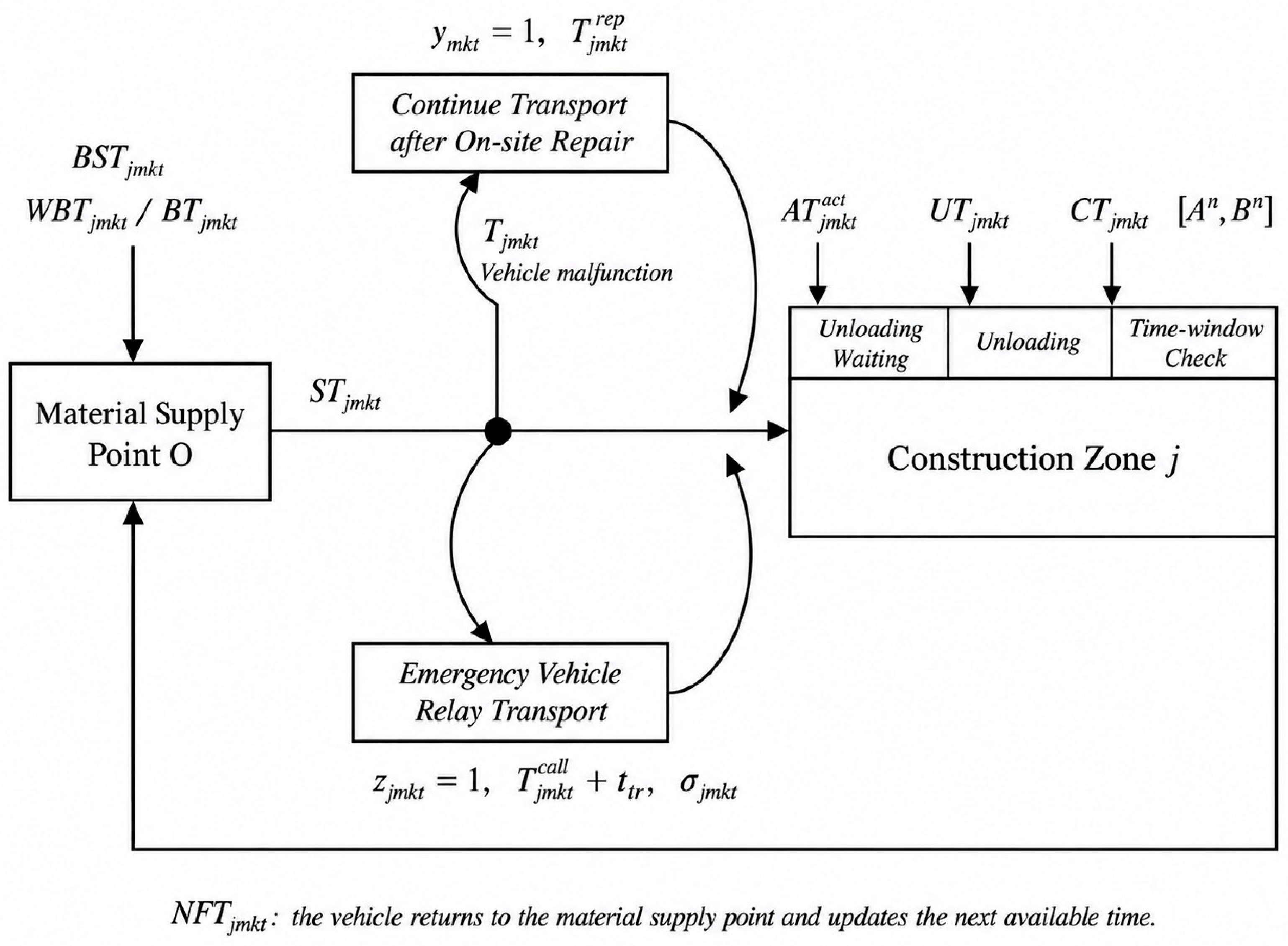
Figure 1 details the material transportation process for a water conservancy project. The parameters involved can be described with reference to the figure as follows. When vehicle i uses unloading equipment h to execute batch (j, m, k), the vehicle’s next-available time upon returning to the material supply point is $R{T}_i^{pre}$ (i.e., $NF{T}_{jhmk}$). If the loading resource for material m is occupied by the preceding vehicle at time $R{T}_i^{pre}$, vehicle i waits until that resource becomes available before loading. Once loading is complete, vehicle i departs from the material supply point at time $S{T}_{ijhmk}$, travels for $T_{oj}^i$, and arrives at construction zone j at time $A{T}_{ijhmk}$. If vehicle i fails in transit at time ${\tau }_{jmk}$, one of two response strategies may be selected. Under on-site repair, vehicle i resumes its trip to construction zone j after a repair duration of $T_{jmk}^{rep}$. Under emergency-vehicle relay, an emergency vehicle carries the material to construction zone j after the response and transshipment periods, while the failed vehicle returns to the material supply point for its next task after being repaired at the malfunction location. The actual arrival time of vehicle i is then $A{T}_{jmk}^{act}$. If the unloading equipment for material m in construction zone j is occupied, vehicle i incurs an unloading waiting time of $W{T}_{jhmk}$ and begins unloading at time $U{T}_{jhmk}$. The unloading duration $U{L}_{jhmk}$ depends on the actual transported quantity $d_{jmk}$, and material handling is completed at time $C{T}_{jhmk}$. Completion before $A_j^m$ incurs site-occupancy time, whereas completion after $B_j^m$ incurs delay penalty time. After unloading, vehicle i leaves construction zone j and returns to the material supply point after a return travel time of $T_{jo}^i$, whereupon its next-available time is updated to $NF{T}_{jhmk}$ (i.e., $R{T}_i^{pre}$).

4.3. Basic Time Variable Relationship During the Transportation Process

A normal material transportation task in a water conservancy project comprises four stages: loading, transportation, unloading, and calculation of deviations from the time window. For concise notation, we define, ${[x]}^{+}=\max \{0,x\}$, which equals x when x > 0 and 0 otherwise.

The recursive time relationships for the loading stage are:

$$\left\{\begin{array}{l}BS{T}_{ijhmk}=\max \{R{T}_i^{pre},A{G}_m^{pre}\}\hfill \\ WB{T}_{ijhmk}=BS{T}_{ijhmk}-R{T}_i^{pre}\hfill \\ B{T}_{ijmk}=b{t}_{im}{d}_{jmk}\hfill \\ S{T}_{ijhmk}=BS{T}_{ijhmk}+B{T}_{ijmk}\hfill \end{array}\right.$$

(1)

Without a malfunction, the vehicle arrival time at the construction zone is:

$$A{T}_{ijhmk}=S{T}_{ijhmk}+T_{oj}^i$$

(2)

After the vehicle reaches the construction zone, the recursive time relationships for unloading are:

$$\left\{\begin{array}{l}U{T}_{jhmk}=\max \{A{T}_{ijhmk}^{act},G{T}_{jh}^{pre}\}\hfill \\ W{T}_{jhmk}=U{T}_{jhmk}-A{T}_{ijhmk}^{act}\hfill \\ U{L}_{jhmk}=u{t}_{hm}{d}_{jmk}\hfill \\ C{T}_{jhmk}=U{T}_{jhmk}+U{L}_{jhmk}\hfill \end{array}\right.$$

(3)

If unloading is completed outside the preferred time window, either site-occupancy time or delay time is incurred:

$$\left\{\begin{array}{l}P{T}_{jhmk}={[A_j^m-C{T}_{jhmk}]}^{+}\hfill \\ D{T}_{jhmk}={[C{T}_{jhmk}-B_j^m]}^{+}\hfill \end{array}\right.$$

(4)

4.4. Time Relationships for Vehicle-Malfunction Emergency Response

When a vehicle fails in transit, no new material demand is generated. Instead, on the condition that the materials loaded onto the failed vehicle continue to their original target construction zone, two response strategies are considered: on-site repair and relay transportation using an external temporary emergency vehicle.

Under the on-site-repair strategy, the failed vehicle continues to its original target construction zone after repair. Its arrival time is:

$$A{T}_{ijhmk}^{rep}={\tau }_{jmk}+T_{jmk}^{rep}+T_{fj}^m$$

(5)

Under the external temporary emergency-vehicle relay strategy, the emergency vehicle reaches the malfunction location, receives the transferred materials, and transports them to the original target construction zone. Its arrival time is:

$$A{T}_{jmk}^{call}={\tau }_{jmk}+T_{jmk}^{call}+t_m^{tr}{d}_{jmk}+T_{fj}^m$$

(6)

After accounting for the malfunction status and response strategy, the actual arrival time of batch (j, m, k) is:

$$A{T}_{jmk}^{act}=(1-F_{jmk}){\displaystyle {\displaystyle \sum _{i=1}^I}{\displaystyle \sum _{h=1}^H{x}_{ijhmk}}}A{T}_{ijhmk}+y_{jmk}{\displaystyle {\displaystyle \sum _{i=1}^I}{\displaystyle \sum _{h=1}^H{x}_{ijhmk}}}A{T}_{ijhmk}^{rep}+z_{jmk}A{T}_{jmk}^{call}$$

(7)

When the external-relay strategy is selected, the failed vehicle cannot return to the supply point until both its own repair and material transshipment have been completed. Its downtime is:

$$P_{jmk}^{call}=\max \{T_{jmk}^{rep},T_{jmk}^{call}+t_m^{tr}{d}_{jmk}\}$$

(8)

The vehicle’s next-available time is:

$$NF{T}_{ijhmk}=\left\{\begin{array}{ll}C{T}_{jhmk}+T_{jo}^i,\hfill & F_{jmk}=0\mathrm{or}{y}_{jmk}=1\hfill \\ {\tau }_{jmk}+P_{jmk}^{call}+T_{fo}^i,\hfill & z_{jmk}=1\hfill \end{array}\right.$$

(9)

4.5. Objective Function

The cost of scheduling construction-material transportation for a water conservancy project consists primarily of vehicle transportation costs, loading and unloading costs, time efficiency costs, and vehicle-malfunction emergency-response costs. Vehicle transportation costs include fixed vehicle costs and travel costs. Loading and unloading costs include unloading-equipment operating costs and loading or unloading waiting costs. Time efficiency costs include the site-occupancy cost caused by early material arrival and the penalty for delayed delivery. Vehicle-malfunction emergency-response costs include repair, vehicle downtime, external emergency-vehicle call-out, and transshipment at the malfunction location. This article aims to minimize total transportation cost, with the objective function being:

$$\min TC=C_{VF}+C_{VT}+C_U+C_W+C_P+C_D+C_F$$

(10)

where $TC$ denotes total transportation cost and $C_{VF}$, $C_{VT}$, $C_U$, $C_W$, $C_P$, $C_D$, and $C_F$ denote the fixed vehicle cost, vehicle travel cost, unloading-equipment operating cost, loading and unloading waiting cost, site-occupancy cost, delay penalty cost, and vehicle-malfunction emergency-response cost, respectively.

• Vehicle transportation costs.

Vehicle transportation costs represent the costs incurred when transport vehicles are activated and operated, including fixed vehicle costs and travel costs. The fixed cost depends on whether a vehicle is activated and is expressed as:

$$C_{VF}={\displaystyle \sum _{i=1}^I{C}_i^D}{s}_i$$

(11)

Vehicle travel cost depends on actual operating time. Without a malfunction, or when transportation continues after on-site repair, the original vehicle completes both the outbound and return trips. When relay transportation by an external temporary emergency vehicle is used, the original failed vehicle is charged only for the time traveled before malfunction and the time required to return to the material supply point after repair. Vehicle travel cost is expressed as:

$$C_{VT}={\displaystyle \sum _{i=1}^I{\displaystyle \sum _{j=1}^J{\displaystyle \sum _{h=1}^H{\displaystyle \sum _{m=1}^M{\displaystyle \sum _{k=1}^{K_{jm}}{x}_{ijhmk}}}}}}{c}_i^T\left[(1-F_{jmk}+y_{jmk})(T_{oj}^i+T_{jo}^i)+z_{jmk}(e_{ijhmk}+T_{fo}^i)\right]$$

(12)

2.

Loading and unloading costs.

Loading and unloading costs primarily comprise unloading-equipment operating costs and loading or unloading waiting costs. The operating cost of unloading equipment depends on its service duration and is expressed as:

$$C_U={\displaystyle \sum _{i=1}^I{\displaystyle \sum _{j=1}^J{\displaystyle \sum _{h=1}^H{\displaystyle \sum _{m=1}^M{\displaystyle \sum _{k=1}^{K_{jm}}{x}_{ijhmk}}}}}}{C}_h^{U}U{L}_{jhmk}$$

(13)

Loading and unloading waiting costs include the costs incurred while a vehicle waits for loading at the material supply point and for unloading after reaching the construction zone. They are expressed as:

$$C_W=\alpha {\displaystyle \sum _{i=1}^I{\displaystyle \sum _{j=1}^J{\displaystyle \sum _{h=1}^H{\displaystyle \sum _{m=1}^M{\displaystyle \sum _{k=1}^{K_{jm}}{x}_{ijhmk}}}}}}\left(WB{T}_{ijhmk}+W{T}_{ijhmk}\right)$$

(14)

3.

Time efficiency costs.

Because construction sites impose explicit timing requirements on material supply, excessively early arrival causes on-site stockpiling and site occupation, whereas late arrival may disrupt subsequent construction activities. Both site-occupancy and delay penalty costs are therefore considered. The site-occupancy cost is:

$$C_P={\displaystyle \sum _{j=1}^J{\displaystyle \sum _{h=1}^H{\displaystyle \sum _{m=1}^M{\displaystyle \sum _{k=1}^{K_{jm}}\beta }}}}P{T}_{jhmk}$$

(15)

The delay penalty cost is:

$$C_D={\displaystyle \sum _{j=1}^J{\displaystyle \sum _{h=1}^H{\displaystyle \sum _{m=1}^M{\displaystyle \sum _{k=1}^{K_{jm}}\delta }}}}D{T}_{jhmk}$$

(16)

4.

Vehicle-malfunction emergency-response costs.

Vehicle-malfunction emergency-response cost is the principal cost component that distinguishes the proposed model from conventional material transportation scheduling models. It includes the fixed malfunction repair cost, failed-vehicle downtime cost under on-site repair, failed-vehicle downtime cost under external relay, external temporary emergency-vehicle call-out cost, and transshipment cost at the malfunction location. It is expressed as:

$$\begin{array}{cc}\hfill C_F& ={\displaystyle \sum _{i=1}^I{\displaystyle \sum _{j=1}^J{\displaystyle \sum _{h=1}^H{\displaystyle \sum _{m=1}^M{\displaystyle \sum _{k=1}^{K_{jm}}{x}_{ijhmk}}}}}}{F}_{jmk}{C}^{rep}\hfill \\ & +{\displaystyle \sum _{i=1}^I{\displaystyle \sum _{j=1}^J{\displaystyle \sum _{h=1}^H{\displaystyle \sum _{m=1}^M{\displaystyle \sum _{k=1}^{K_{jm}}{x}_{ijhmk}}}}}}{y}_{jmk}{c}_i^P{T}_{jmk}^{rep}\hfill \\ & +{\displaystyle \sum _{i=1}^I{\displaystyle \sum _{j=1}^J{\displaystyle \sum _{h=1}^H{\displaystyle \sum _{m=1}^M{\displaystyle \sum _{k=1}^{K_{jm}}{x}_{ijhmk}}}}}}{z}_{jmk}{c}_i^P{P}_{jmk}^{call}\hfill \\ & +{\displaystyle \sum _{j=1}^J{\displaystyle \sum _{h=1}^H{\displaystyle \sum _{m=1}^M{\displaystyle \sum _{k=1}^{K_{jm}}{z}_{jmk}}}}}\left(C^{call}+c_m^{tr}{d}_{jmk}\right)\hfill \end{array}$$

(17)

4.6. Constraints

To ensure that the model solution satisfies the organizational requirements of construction-material transportation at water conservancy sites, constraints are imposed on basic transportation feasibility, emergency responses to vehicle malfunctions, time windows, material release management, and variable domains.

• Basic transportation feasibility constraints.

In construction-material transportation for water conservancy projects, the demand for each material in every construction zone must be fulfilled collectively by multiple transportation batches, and each batch must be assigned a specific transport vehicle and item of unloading equipment. Vehicle capacity, vehicle–material compatibility, unloading-equipment compatibility, and vehicle activation status all affect task assignment.

$$\left\{\begin{array}{ll}{\displaystyle \sum _{k=1}^{K_{jm}}{d}_{jmk}}=D_{jm},\hfill & \forall j,m,\hfill \\ {\displaystyle \sum _i{\displaystyle \sum _h{x}_{ijhmk}}}=1,\hfill & \forall j,m,k,\hfill \\ d_{jmk}{x}_{ijhmk}\le Q_i,\hfill & \forall i,j,h,m,k,\hfill \\ x_{ijhmk}\le {\lambda }_{im},\hfill & \forall i,j,h,m,k,\hfill \\ x_{ijhm}\le {\mu }_{hm},\hfill & \forall i,j,h,m,k,\hfill \\ x_{ijhkm}\le s_i,\hfill & \forall i,j,h,m,k.\hfill \end{array}\right.$$

(18)

2.

Emergency-response constraints for vehicle malfunctions.

This study considers in-transit malfunctions, meaning that the vehicle has left the material supply point but has not yet reached the target construction zone under normal operation. A malfunction before departure can be handled by replacing or repairing the vehicle, whereas a malfunction after material arrival no longer affects delivery of that batch. The malfunction time must therefore lie between the vehicle’s departure and normal arrival times. After a malfunction, only two response strategies are considered: continuing transportation after on-site repair and relay transportation using an external temporary emergency vehicle.

$$\left\{\begin{array}{ll}S{T}_{ijhmk}\le {\tau }_{jmk}\le A{T}_{ijhmk},\hfill & \forall i,j,h,m,k\mid x_{ijhmk}=1,F_{jmk}=1,\hfill \\ y_{jmk}+z_{jmk}=F_{jmk},\hfill & \forall j,m,k.\hfill \end{array}\right.$$

(19)

3.

Time-window and material release management constraints.

Construction sites have explicit delivery time requirements for each material type. If unloading is completed outside the acceptable time window, the construction zone may be left waiting for materials, equipment and labor may remain idle, or on-site operations may become unbalanced. Accordingly, unloading of every batch must be completed within its acceptable time window. Moreover, a vehicle malfunction may change only the transportation mode and arrival time of the failed batch and the subsequent availability of the failed vehicle; it must not change the original batch, material quantity, or target construction zone.

$$\left\{\begin{array}{l}{E}_j^m\le C{T}_{jhmk}\le L_j^m,\forall j,h,m,k,\hfill \\ d_{jmk}^{out}=d_{jmk}^{arrive}=d_{jmk},\forall j,m,k.\hfill \end{array}\right.$$

(20)

4.

Variable value constraints.

Vehicle assignment, vehicle activation, and malfunction-response strategy selection variables are binary. Malfunction status is a binary parameter specified by the malfunction scenario. Transportation quantities and all time variables are nonnegative.

$$\left\{\begin{array}{l}{x}_{ijhmk},s_i,y_{jmk},z_{jmk}\in \{0,1\},\hfill \\ F_{jmk}\in \{0,1\},\hfill \\ d_{jmk},S{T}_{ijhmk},A{T}_{ijhmk},A{T}_{jmk}^{act},WB{T}_{ijhmk},W{T}_{jhmk},U{T}_{jhmk},C{T}_{jhmk},P{T}_{jhmk},D{T}_{jhmk},NF{T}_{ijhmk}\ge 0\hfill \end{array}\right.$$

(21)

5. Design of the Adaptive Hill-Climbing Genetic Algorithm

The material transportation scheduling model formulated above simultaneously involves transportation-batch generation, vehicle assignment, unloading-equipment assignment, transportation sequence optimization, time-window constraints, and selection of a vehicle-malfunction response strategy. It is therefore a typical combinatorial optimization problem whose solution space expands rapidly as the numbers of construction zones, vehicles, and transportation batches increase, making conventional exact methods difficult to apply. Accordingly, this study employs an adaptive hill-climbing genetic algorithm. Relative to the conventional GA and HCGA with fixed genetic parameters, AHCGA adaptively adjusts crossover and mutation probabilities over the evolutionary process and applies hill-climbing local search to high-quality individuals. In addition, the malfunction-response strategy is incorporated directly into the chromosome representation, and only the failed task and the affected unexecuted tasks are dynamically rescheduled after a malfunction. A complete transportation schedule X is encoded as a chromosome represented by:

$$[X=\left(X_1,X_2,X_3,X_4,X_5\right)]$$

(22)

where $X_1$ denotes the transportation batches and their quantities generated from total material demand in the construction zones and vehicle capacities; $X_2$ denotes the batch-execution sequence; $X_3$ denotes the vehicle assignment result; $X_4$ denotes the unloading-equipment assignment result; and $X_5$ denotes the malfunction-response strategy, where 0 indicates continued transportation after on-site repair and 1 indicates relay transportation by an external temporary emergency vehicle. For a transportation task without a malfunction, $X_5$ is not used in the calculation.

During initial population generation, the algorithm automatically creates transportation batches according to the total demand for each material type in the construction zones and vehicle capacities and then randomly generates transportation sequences, vehicle assignments, and unloading-equipment assignments. To ensure individual feasibility, the algorithm repairs vehicle overload, vehicle–material incompatibility, unloading-equipment incompatibility, and acceptable-time-window violations. If an individual remains infeasible after repair, a penalty is added during fitness evaluation.

During individual decoding, the algorithm follows the batch-execution sequence and calculates, for each batch, the loading start time, vehicle departure time, actual arrival time, unloading start time, unloading completion time, and vehicle next-available time. The total transportation cost of the corresponding schedule is then evaluated using the total cost function. An individual X in the genetic algorithm represents a complete material transportation schedule, including the batches and their transportation quantities, batch-execution sequence, vehicle assignments, unloading-equipment assignments, and malfunction-response strategies. Let the total cost of individual X be $TC\left(X\right)$, the constraint violation penalty be $P\left(X\right)$, and the penalty coefficient be $M$. The fitness function is:

$$Fit(X)={\displaystyle \frac{1}{TC(X)+MP(X)}}$$

(23)

When a transportation schedule satisfies the vehicle capacity, material compatibility, unloading-equipment compatibility, time, and other constraints, $P\left(X\right)=0$; otherwise, a penalty is assigned according to the degree of violation. Because a lower total cost corresponds to higher fitness, the algorithm preferentially retains low-cost schedules that satisfy the constraints.

The genetic operators comprise selection, crossover, and mutation. High-quality individuals are retained through a combination of roulette wheel selection and elitism. Crossover and mutation primarily adjust the transportation sequence, vehicle assignments, unloading-equipment assignments, and malfunction-response strategy. To balance global search capability in the early stage with convergence stability in the later stage, adaptive crossover probability $P_c(g)$ and mutation probability $P_m(g)$ are used:

$$P_c(g)=P_c^{max}-{\displaystyle \frac{g}{G_{\max }}}\left(P_c^{max}-P_c^{min}\right)$$

(24)

$$P_m(g)=P_m^{max}-{\displaystyle \frac{g}{G_{\max }}}\left(P_m^{max}-P_m^{min}\right)$$

(25)

where $g$ is the current iteration, $G_{\max }$ is the maximum number of iterations, $P_c^{max}$ and $P_c^{min}$ are the maximum and minimum crossover probabilities, respectively, and $P_m^{max}$ and $P_m^{min}$ are the maximum and minimum mutation probabilities, respectively.

After the genetic operations, hill-climbing local search is applied to high-quality individuals. Candidate solutions are locally improved by exchanging task positions in the transportation sequence or by reselecting vehicles or unloading equipment. A candidate is accepted if it satisfies all constraints and reduces total cost; otherwise, the incumbent solution is retained.

After a no-malfunction baseline schedule is obtained, one transportation task is selected as the failed task and the on-site-repair and external temporary emergency-vehicle relay strategies are evaluated separately. Tasks already started or completed before the malfunction remain fixed. For the failed task and affected subsequent tasks that have not yet started, vehicle availability, unloading-equipment availability, actual arrival time, and unloading completion time are recalculated to generate a post-malfunction schedule. Vehicle assignments for affected unexecuted tasks are reoptimized according to post-malfunction vehicle availability rather than being fixed to the baseline plan; consequently, available vehicles from the existing fleet may undertake subsequent affected tasks. If a response strategy causes any task to complete unloading outside its acceptable time window, that strategy is deemed infeasible and excluded from the final recommendation. Among the feasible alternatives, the strategy with the lower total cost is selected as the malfunction-response scheduling solution.

In summary, the AHCGA solution procedure consists of the following steps: (1) generate transportation batches from material demand and vehicle capacities and initialize the population; (2) decode and repair each individual and evaluate total transportation cost and fitness; (3) perform selection, adaptive crossover, and mutation; (4) apply hill-climbing local search to high-quality individuals; (5) output the no-malfunction baseline schedule once the stopping criterion is satisfied; and (6) after a vehicle malfunction, update the relevant resource states and reoptimize the failed task together with the affected unexecuted tasks.

6. Case Study

6.1. Case Background Description

A material transportation scheduling problem from a water conservancy project is used as the case study. The construction site contains one material supply point O that supplies sand and gravel, rockfill, reinforcing steel, formwork, and other construction materials to seven construction zones. These zones differ in construction activities, material demands, transportation distances, unloading-equipment conditions, and timing requirements. An inappropriate transportation schedule may therefore cause vehicle waiting, premature material stockpiling, delayed delivery of critical materials, and disruption of subsequent construction activities.

The seven construction zones are the J1 channel lining zone, J2 sluice floor zone, J3 embankment reinforcement zone, J4 pumping station structural zone, J5 diversion open-channel zone, J6 stilling basin zone, and J7 temporary road and construction platform zone. Depending on its construction activities, each zone requires one to four material types.

The case study follows a three-stage solution procedure: no-malfunction baseline scheduling, failed-task selection, and emergency-response comparison. First, a baseline transportation schedule is generated without considering vehicle malfunctions. Second, one transportation task in the baseline schedule is selected as the failed task. Finally, total transportation costs are calculated separately for continued transportation after on-site repair and for relay transportation using an external temporary emergency vehicle, and the feasible strategy with the lower total cost is selected as the malfunction-response scheduling solution.

6.2. Case Data and Parameter Settings

Four construction-material types commonly used in water conservancy projects are considered: sand and gravel, rockfill, reinforcing steel, and formwork. The applicable transport vehicles and unloading methods differ by material type. Sand and gravel and rockfill are transported primarily by dump trucks, whereas reinforcing steel and formwork are transported primarily by flatbed trucks. Multipurpose trucks may carry several material types when vehicle resources are constrained. The material demands and preferred time windows are reported in

Table 3. Material demands and time windows.

ID	$\mathit{j}$	$\mathit{m}$	${\mathit{D}}_{\mathit{j}\mathit{m}}$	${\mathit{T}}_{\mathit{o}\mathit{j}}^{\mathit{i}}$/${\mathit{T}}_{\mathit{j}\mathit{o}}^{\mathit{i}}$	$[{\mathit{A}}_{\mathit{j}}^{\mathit{m}},{\mathit{B}}_{\mathit{j}}^{\mathit{m}}]$
R1	J1	sand and gravel	80	15/12	09:00–10:30
R2	J1	formwork	18	15/12	10:00–11:30
R3	J2	reinforcing steel	32	22/18	09:30–11:30
R4	J2	formwork	20	22/18	10:30–13:30
R5	J2	sand and gravel	40	22/18	11:00–13:00
R6	J3	rockfill	20	28/24	09:30–15:30
R7	J4	reinforcing steel	32	32/27	10:30–13:00
R8	J4	formwork	34	32/27	11:00–13:30
R9	J4	sand and gravel	40	32/27	09:00–17:00
R10	J4	rockfill	28	32/27	10:00–17:30
R11	J5	sand and gravel	20	25/21	11:00–13:30
R12	J5	rockfill	45	25/21	09:00–15:00
R13	J6	reinforcing steel	40	30/25	12:30–14:30
R14	J6	formwork	16	30/25	13:00–15:00
R15	J6	sand and gravel	25	30/25	10:00–17:30
R16	J7	sand and gravel	20	38/32	09:00–16:00
R17	J7	rockfill	25	38/32	13:30–17:30

.

The case study includes eight transport vehicles: dump trucks, flatbed trucks, and multipurpose trucks. Their parameters are listed in

Table 4. Transport vehicle parameters.

ID	Type	${\mathit{Q}}_{\mathit{i}}$	${\mathit{C}}_{\mathit{i}}^{\mathit{D}}$	${\mathit{c}}_{\mathit{i}}^{\mathit{T}}$	${\mathit{c}}_{\mathit{i}}^{\mathit{P}}$	Compatible Materials
V1	dump truck	30	300	3.2	0.8	sand and gravel and rockfill
V2	dump truck	28	280	3.0	0.7	sand and gravel and rockfill
V3	dump truck	25	260	2.8	0.7	sand and gravel and rockfill
V4	flatbed truck	20	260	2.8	0.7	reinforcing steel and formwork
V5	flatbed truck	20	260	2.8	0.7	reinforcing steel and formwork
V6	flatbed truck	15	230	2.6	0.6	reinforcing steel and formwork
V7	multipurpose truck	20	300	3.0	0.8	sand and gravel, rockfill, reinforcing steel, and formwork
V8	multipurpose truck	20	300	3.0	0.8	sand and gravel, rockfill, reinforcing steel, and formwork

.

Each construction zone is equipped with the corresponding unloading equipment. The equipment parameters are listed in

Table 5. Unloading-equipment parameters.

ID	$\mathit{j}$	Compatible Materials	${\mathit{C}}_{\mathit{h}}^{\mathit{U}}$
D1	J1	sand and gravel, rockfill, and formwork	1.6
D2	J2	reinforcing steel, formwork, and sand and gravel	1.8
D3	J3	sand and gravel and rockfill	1.5
D4	J4	sand and gravel, rockfill, reinforcing steel, and formwork	2.0
D5	J5	sand and gravel and rockfill	1.5
D6	J6	reinforcing steel, formwork, and sand and gravel	1.8
D7	J7	sand and gravel and rockfill	1.5

.

Loading, unloading, and transshipment efficiencies at the malfunction location differ by material type. Loading, unloading, and transshipment times are assumed to be proportional to the actual quantity transported in each batch. The corresponding material-handling parameters are listed in

Table 6. Material-handling parameters.

$\mathit{m}$	$\mathit{b}{\mathit{t}}_{\mathit{i}\mathit{m}}$	$\mathit{u}{\mathit{t}}_{\mathit{h}\mathit{m}}$	${\mathit{t}}_{\mathit{m}}^{\mathit{t}\mathit{r}}$	${\mathit{c}}_{\mathit{m}}^{\mathit{t}\mathit{r}}$
sand and gravel	0.60	0.55	0.40	2
rockfill	0.70	0.65	0.50	3
reinforcing steel	1.00	0.90	0.80	4
formwork	0.80	0.85	0.60	3

.

Scheduling begins at 08:00. The waiting cost, early-arrival site-occupancy cost, delay penalty cost, and malfunction-response cost parameters are listed in

Table 7. Cost parameters.

Parameter	Value
Scheduling start time	8:00
Waiting cost	CNY 4.0/min
Early-arrival site-occupancy cost	CNY 4.0/min
Delay penalty cost	CNY 8.0/min
Fixed malfunction repair cost	CNY 200/call
External emergency-vehicle call-out cost	CNY 350/call

.

6.3. Algorithm Parameter Settings

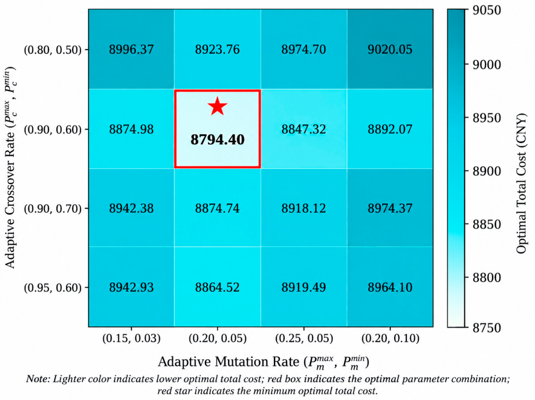
The model incorporates several classes of constraints, including vehicle capacity, vehicle–material compatibility, unloading-equipment compatibility, acceptable time windows, and malfunction-response strategy selection. Inappropriate parameter settings may therefore lead to premature convergence or insufficient exploration of the feasible solution space. To improve the stability and reproducibility of AHCGA and to evaluate the effects of adaptive crossover and mutation probabilities on solution performance, parameter pretests are conducted before the formal optimization using a one-factor-at-a-time approach. The population size is fixed at 100, the maximum number of iterations at 150, and the number of hill-climbing searches at 10. AHCGA is then evaluated under the tested combinations of adaptive crossover and mutation probabilities. Each parameter combination is run independently 10 times, and the best total cost across the repeated runs is used as the parameter selection criterion. The results are shown in Figure 2.

As shown in Figure 2, when $P_c^{max}=0.90$, $P_c^{min}=0.60$, $P_m^{max}=0.20$, and $P_m^{min}=0.05$, the model obtains a minimum total cost of CNY 8794.40, the lowest among all tested combinations. This combination maintains the population’s global search capability while using moderate mutation to improve its ability to escape local optima, thereby avoiding premature convergence. These crossover and mutation probability parameters are therefore used in the subsequent optimization.

6.4. Ablation and Stability Analysis of Algorithmic Enhancement Mechanisms

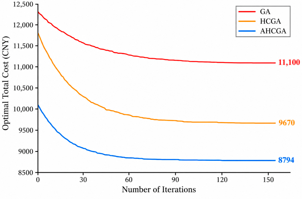
To quantify the contribution of the different enhancement mechanisms incorporated in AHCGA, GA, HCGA, and AHCGA are treated as progressively enhanced variants in an ablation analysis. GA serves as the baseline algorithm; HCGA augments GA with hill-climbing local search to strengthen local exploitation; and AHCGA further introduces adaptive crossover and mutation to balance global exploration and local exploitation over the evolutionary process. Under identical case data and parameter settings, the three algorithms are evaluated using the same set of 30 random seeds, and the best total cost obtained in each run is recorded. In addition to descriptive statistics, Wilcoxon signed-rank tests are used to compare AHCGA with GA and HCGA at a significance level of 0.05. The results are reported in

Table 8. Ablation and statistical test results for GA, HCGA, and AHCGA.

Algorithm	Best Total Cost (CNY)	Mean Total Cost (CNY)	Standard Deviation	Total Earliness (min)	Total Delay Time (min)	Mean Runtime (s)	p-Value	Effect Size r
GA	11,106.70	12,223.78	1362.83	126	528	0.08	<0.001	0.871
HCGA	9670.53	10,165.69	627.56	36	26	0.13	<0.001	0.774
AHCGA	8794.40	9179.86	476.33	7	0	0.18	-	-

Note: Each algorithm was run 30 times using the same set of random seeds. The p-values and effect sizes r correspond to Wilcoxon signed-rank comparisons of GA and HCGA against AHCGA, respectively. A value of p < 0.05 indicates statistical significance, and r > 0.5 indicates a large effect.

and Figure 3.

Table 8 and Figure 3 show the incremental effects of the different algorithmic enhancement mechanisms. Across the 30 runs, the mean total costs of GA, HCGA, and AHCGA are CNY 12,223.78, CNY 10,165.69, and CNY 9179.86, respectively, with corresponding standard deviations of 1362.83, 627.56, and 476.33. Relative to GA, incorporating hill-climbing local search into HCGA substantially reduces both the mean total cost and the dispersion of the solutions. Building on HCGA, the adaptive crossover and mutation mechanisms in AHCGA further reduce the mean total cost to CNY 9179.86 and the standard deviation to 476.33. The Wilcoxon signed-rank tests show statistically significant cost differences between AHCGA and both GA and HCGA (p < 0.001 for both comparisons), with effect sizes of 0.871 and 0.774, respectively, both indicating large effects. AHCGA also attains the lowest best total cost, CNY 8794.40, while reducing total earliness to 7 min and total delay to zero. Its mean runtime is 0.18 s, compared with 0.08 s for GA and 0.13 s for HCGA. The additional computational effort results primarily from adaptive parameter updates and hill-climbing local search. Overall, the ablation results provide statistical support for the contribution of both hill-climbing local search and adaptive genetic operations to solution quality and stability, with a limited increase in computational time.

The baseline case contains seven construction zones, eight transport vehicles, and 26 transportation batches. The chromosome representation, constraint-checking procedure, and post-malfunction rescheduling mechanism are constructed according to the actual numbers of transportation tasks, vehicles, and unloading equipment rather than a fixed problem size. Accordingly, the proposed model and algorithmic framework are structurally extensible to cases with additional construction zones, vehicles, or transportation batches.

6.5. Analysis of Optimization Results

To present the no-malfunction material transportation schedule generated by the model,

Table 9. No-malfunction material transportation schedule.

(j, m, k)	$\mathit{i}$	$\mathit{S}{\mathit{T}}_{\mathit{i}\mathit{j}\mathit{h}\mathit{m}\mathit{k}}$	$\mathit{A}{\mathit{T}}_{\mathit{i}\mathit{j}\mathit{h}\mathit{m}\mathit{k}}$	$\mathit{U}{\mathit{T}}_{\mathit{j}\mathit{h}\mathit{m}\mathit{k}}$	$\mathit{C}{\mathit{T}}_{\mathit{j}\mathit{h}\mathit{m}\mathit{k}}$	$\mathit{N}\mathit{F}{\mathit{T}}_{\mathit{j}\mathit{h}\mathit{m}\mathit{k}}$
J1-sand and gravel-1	V1	08:20	08:35	08:35	08:53	09:05
J1-formwork-1	V5	08:15	08:30	09:58	10:14	10:26
J1-sand and gravel-3	V7	08:30	08:45	08:53	09:02	09:14
J1-sand and gravel-2	V1	09:25	09:40	09:40	09:58	10:10
J2-reinforcing steel-2	V7	09:26	09:48	09:48	09:59	10:17
J2-sand and gravel-1	V1	10:30	10:52	10:52	11:10	11:28
J2-reinforcing steel-1	V7	10:37	10:59	11:10	11:28	11:46
J4-formwork-1	V5	10:42	11:14	11:14	11:31	11:58
J4-reinforcing steel-2	V6	10:49	11:21	11:31	11:42	12:09
J4-reinforcing steel-1	V4	11:09	11:41	11:42	12:00	12:27
J2-sand and gravel-2	V1	11:33	11:55	11:55	12:00	12:18
J5-sand and gravel-1	V7	11:58	12:23	12:23	12:34	12:55
J2-formwork-1	V5	12:14	12:36	12:36	12:53	13:11
J7-sand and gravel-1	V3	12:10	12:48	12:48	12:59	13:31
J4-formwork-2	V6	12:26	12:58	12:58	13:10	13:37
J5-rockfill-1	V1	12:41	13:06	13:06	13:27	13:48
J6-reinforcing steel-1	V4	12:47	13:17	13:17	13:35	14:00
J5-rockfill-2	V7	13:05	13:30	13:30	13:39	14:00
J6-reinforcing steel-2	V5	13:31	14:01	14:01	14:19	14:44
J4-sand and gravel-2	V3	13:36	14:08	14:08	14:13	14:40
J4-sand and gravel-1	V1	14:08	14:40	14:40	14:58	15:25
J3-rockfill-1	V7	14:14	14:42	14:42	14:55	15:19
J6-formwork-1	V4	14:13	14:43	14:43	14:57	15:22
J6-sand and gravel-1	V3	14:55	15:25	15:25	15:39	16:04
J4-rockfill-1	V1	15:45	16:17	16:17	16:36	17:03
J7-rockfill-1	V3	16:22	17:00	17:00	17:17	17:49

reports the schedule corresponding to the best solution obtained above.

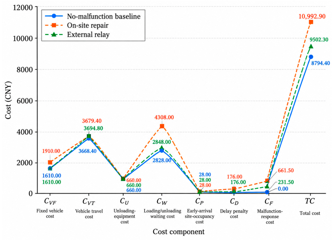
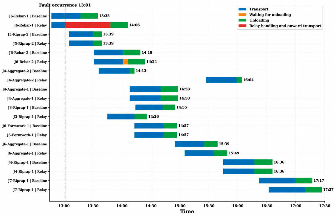
Using the no-malfunction baseline schedule, task J6-reinforcing steel-1 is selected as the failed task. The malfunction occurs at 13:01; the on-site response and repair time is 45 min; the external emergency vehicle requires 15 min to reach the malfunction location; and the failed vehicle requires 15 min to return to the material supply point after repair. After the malfunction, the model fixes either the on-site-repair or external-relay strategy and, under each strategy, reoptimizes the subsequent task sequence, vehicle assignments, and unloading-equipment assignments. The resulting emergency-response costs are compared in Figure 4.

As shown in Figure 4, the total costs of the on-site-repair and external-relay strategies are CNY 10,992.90 and CNY 9502.30, respectively. Because the external temporary emergency-vehicle relay strategy yields the lower total transportation cost, it is selected as the recommended response for the baseline malfunction scenario.

To clearly illustrate the post-malfunction rescheduling mechanism and the direct effect of the vehicle malfunction on the baseline schedule, only the failed task and the affected subsequent tasks are reported in the rescheduling results. Using the recommended external-relay strategy as an example,

Table 10. Post-malfunction material transportation rescheduling results.

(j, m, k)	$\mathit{i}$	$\mathit{S}{\mathit{T}}_{\mathit{i}\mathit{j}\mathit{h}\mathit{m}\mathit{k}}$	$\mathit{A}{\mathit{T}}_{\mathit{j}\mathit{m}\mathit{k}}^{\mathit{a}\mathit{c}\mathit{t}}$	$\mathit{U}{\mathit{T}}_{\mathit{j}\mathit{h}\mathit{m}\mathit{k}}$	$\mathit{C}{\mathit{T}}_{\mathit{j}\mathit{h}\mathit{m}\mathit{k}}$	$\mathit{N}\mathit{F}{\mathit{T}}_{\mathit{j}\mathit{h}\mathit{m}\mathit{k}}$
J6-reinforcing steel-1	Emergency vehicle	12:47	13:48	13:48	14:06	14:01
J5-rockfill-2	V7	13:05	13:30	13:30	13:39	14:00
J6-reinforcing steel-2	V5	13:31	14:01	14:06	14:24	14:49
J3-rockfill-1	V3	13:45	14:13	14:13	14:26	14:50
J4-sand and gravel-1	V1	14:08	14:40	14:40	14:58	15:25
J6-formwork-1	V7	14:13	14:43	14:43	14:57	15:22
J6-sand and gravel-1	V3	15:05	15:35	15:35	15:49	16:14
J4-sand and gravel-2	V7	15:27	15:59	15:59	16:04	16:31
J4-rockfill-1	V1	15:45	16:17	16:17	16:36	17:03
J7-rockfill-1	V3	16:32	17:10	17:10	17:27	17:59

presents the post-malfunction schedule, and Figure 5 shows the Gantt chart for the affected rescheduled tasks.

Table 9 and Figure 4 show that the model generates a feasible material transportation schedule under the no-malfunction baseline scenario, with every transportation batch completing unloading within its acceptable time window. After an in-transit malfunction occurs in batch J6-reinforcing steel-1 at 13:01, the model performs post-malfunction rescheduling separately under the on-site-repair and external temporary emergency-vehicle relay strategies. Their total costs are CNY 10,992.90 and CNY 9502.30, respectively; external relay therefore reduces total cost by CNY 1490.60, or 13.56%. Although external relay introduces additional emergency-vehicle call-out and transshipment costs, it shortens the time required to complete delivery of the affected materials and mitigates the effect of delayed vehicle availability on subsequent tasks, resulting in a lower total transportation cost under the baseline malfunction scenario.

Table 10 and Figure 5 further show that an in-transit vehicle malfunction affects not only the failed batch itself but also subsequent transportation tasks through changes in the vehicle’s next-available time, unloading-equipment occupancy, and task execution sequence. By resequencing the failed task and affected subsequent tasks and reassigning vehicles, the model ensures that materials already released from inventory continue to their original target construction zones while preventing duplicate material requisitions and double counting of task quantities.

6.6. Sensitivity and Scenario Applicability Analysis of Malfunction-Response Strategies

(1) Sensitivity Analysis of Key Emergency-Response Parameters.

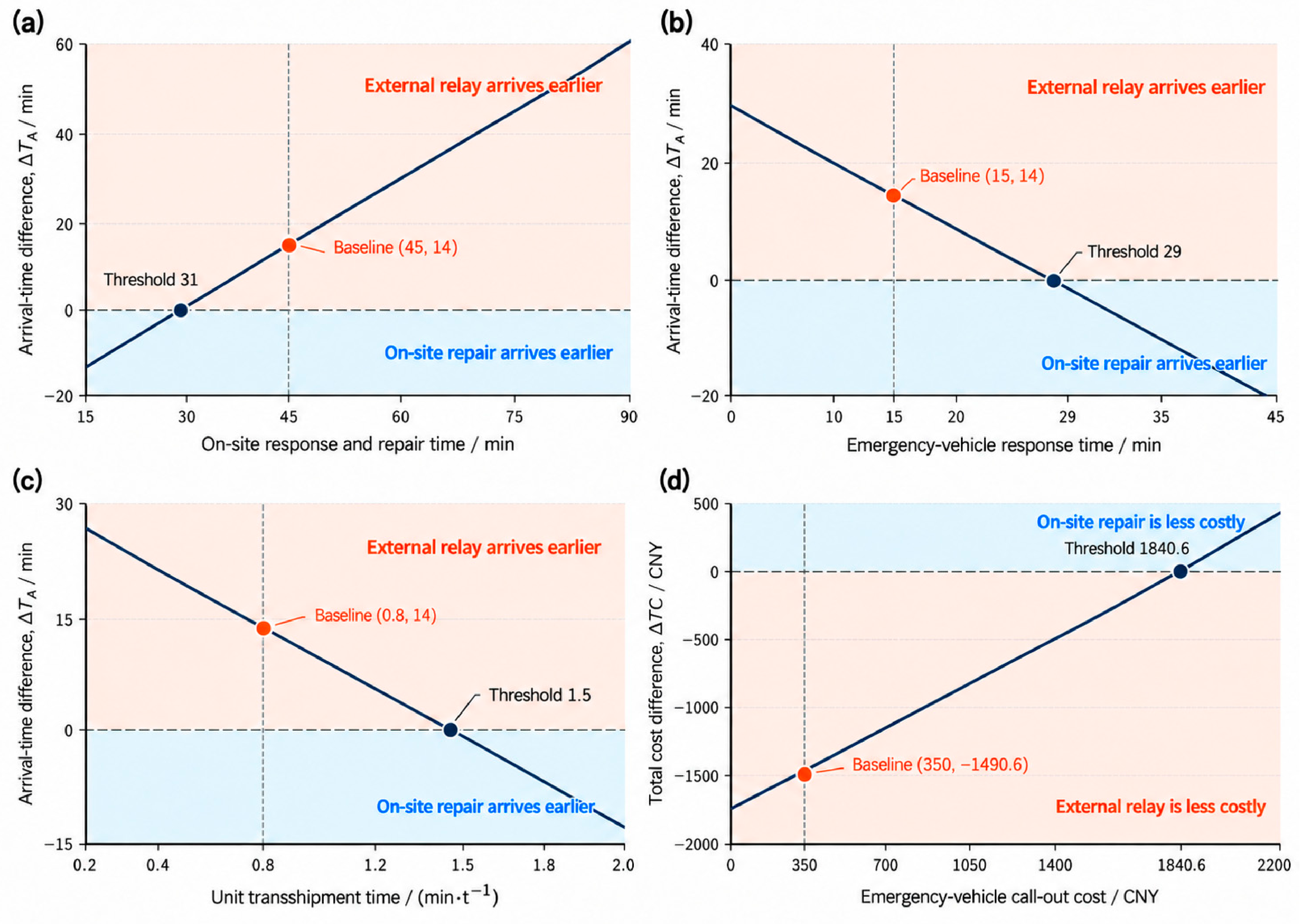
The baseline case shows that for batch J6-reinforcing steel-1 under the specified malfunction parameters, the external temporary emergency-vehicle relay strategy yields a lower total cost than on-site repair. This result, however, is specific to the adopted parameter combination and does not imply that either response strategy is universally dominant. Accordingly, on-site response and repair time, emergency-vehicle response time, unit transshipment time, and emergency-vehicle call-out cost are treated as key uncertain parameters. With the failed task, transportation quantity, and remaining travel time held constant, these parameters are perturbed individually to evaluate how field-level uncertainty affects the timeliness and economic performance of the two response strategies.

For the first three time parameters, the difference in arrival time between the two strategies is defined from Equations (5) and (6) as:

$$\Delta T_A={\mathit{AT}}^{\mathit{rep}}-{\mathit{AT}}^{\mathit{call}}$$

(26)

where $\Delta T_A>0$ indicates that external relay reaches the construction zone earlier, whereas $\Delta T_A<0$ indicates that on-site repair arrives earlier. For the emergency-vehicle call-out cost, the difference in total cost is defined as:

$$\Delta TC={\mathit{TC}}^{\mathit{call}}-{\mathit{TC}}^{\mathit{rep}}$$

(27)

where $\Delta TC<0$ indicates that external relay has the lower cost, whereas $\Delta TC>0$ indicates that on-site repair has the lower cost. The sensitivity analysis results are shown in Figure 6.

As shown in Figure 6a–c, increasing the on-site response and repair time enlarges the timeliness advantage of external relay, whereas increasing the emergency-vehicle response time or unit transshipment time reduces that advantage. Under the case study settings, the critical values of on-site response and repair time, emergency-vehicle response time, and unit transshipment time are 31 min, 29 min, and 1.5 min/t, respectively. Under the baseline scenario, external relay reaches the target construction zone 14 min earlier than on-site repair.

Figure 6d shows a positive relationship between emergency-vehicle call-out cost and the total cost difference between the two response strategies. At a call-out cost of CNY 350/call, external relay costs CNY 1490.60 less than on-site repair. The two strategies have equal total costs when the call-out cost reaches CNY 1840.60/call; above this threshold, the cost advantage shifts progressively toward on-site repair.

External relay is therefore more suitable when on-site response and repair take longer, emergency vehicles can respond rapidly, transshipment efficiency is high, and call-out cost remains moderate. Conversely, on-site repair is more appropriate when the malfunction can be resolved quickly, when the emergency-vehicle response is slow, or when external call-out cost is high. The final response should still be selected from the total cost obtained after dynamic rescheduling, subject to the acceptable time-window constraints. These results further indicate that the preferred response is sensitive to uncertainty in repair time, emergency response, transshipment efficiency, and call-out cost. Near the identified threshold values, relatively small changes in field conditions may reverse the relative advantage of the two strategies. Response decisions should therefore be updated using post-malfunction field information rather than being determined from a single fixed parameter set.

(2) Strategy Applicability under Different Failed-Task Scenarios.

The preceding sensitivity analysis fixes J6-reinforcing steel-1 as the failed task and examines how changes in emergency-response parameters affect the two response strategies. To assess the applicability of the strategies under different failed-task conditions, four representative tasks are selected from the no-malfunction baseline schedule: J1-sand and gravel-1, J5-sand and gravel-1, J6-reinforcing steel-1, and J7-rockfill-1. These tasks differ in outbound travel time, preferred time-window width, and position within the baseline schedule, thereby enabling comparison of the two response strategies under different transportation task conditions.

The outbound travel times of J1-sand and gravel-1, J5-sand and gravel-1, J6-reinforcing steel-1, and J7-rockfill-1 are 15, 25, 30, and 38 min, respectively. Their preferred time windows are 09:00–10:30, 11:00–13:30, 12:30–14:30, and 13:30–17:30, corresponding to time-window widths of 90, 150, 120, and 240 min. The four tasks also occur at early, middle, and late positions in the baseline schedule, allowing the effect of scheduling position on the propagation of malfunction-related disruptions to subsequent tasks to be examined.

To ensure comparability across failed-task scenarios, the principal emergency-response parameters are held constant: the on-site response and repair time is set to 45 min, the external emergency-vehicle response time is set to 15 min, and each malfunction is assumed to occur at approximately the midpoint of the outbound trip. For each failed task, continued transportation after on-site repair and relay transportation using an external temporary emergency vehicle are evaluated separately. The failed task and the affected subsequent unexecuted tasks are then rescheduled by reoptimizing task sequencing, vehicle assignments, and unloading-equipment assignments. The resulting total transportation costs are compared in

Table 11. Comparison of emergency-response strategies under different failed-task scenarios.

(j, m, k)	${\mathit{T}}_{\mathit{o}\mathit{j}}^{\mathit{i}}$	Time-Window Width (min)	Schedule Position	On-Site Repair Total Cost (CNY)	External Relay Total Cost (CNY)	Selected Response
J1-sand and gravel-1	15	90	Early	11,806.20	9144.60	External relay
J5-sand and gravel-1	25	150	Middle	10,777.60	11,389.20	On-site repair
J6-reinforcing steel-1	30	120	Middle	10,992.90	9502.30	External relay
J7-rockfill-1	38	240	Late	11,066.50	9630.70	External relay

.

Table 11 shows that the relative economic performance of the two response strategies varies across failed-task scenarios. For J1-sand and gravel-1, J6-reinforcing steel-1, and J7-rockfill-1, the external-relay strategy yields total costs of CNY 9144.60, CNY 9502.30, and CNY 9630.70, respectively, representing reductions of CNY 2661.60 (22.54%), CNY 1490.60 (13.56%), and CNY 1435.80 (12.97%) relative to on-site repair. External relay is therefore selected in these three scenarios. By contrast, for J5-sand and gravel-1, the on-site-repair strategy has a total cost of CNY 10,777.60, which is CNY 611.60 (5.37%) lower than external relay; on-site repair is therefore selected for this scenario.

Comparison across the four failed tasks indicates that the total cost difference between the two response strategies does not vary monotonically with outbound travel time or preferred time-window width. For example, external relay remains less costly for the relatively short-distance, narrower-window J1 task; on-site repair is less costly for J5 under intermediate travel time and time-window conditions; and external relay again provides a lower total transportation cost for the longer-distance, wider-window J7 task. The preferred response therefore cannot be determined from outbound travel time, time-window width, or schedule position alone. It is also influenced by post-malfunction changes in vehicle next-available times, unloading-equipment occupancy, and subsequent task sequencing.

Taken together, the parameter sensitivity analysis and the failed-task scenario comparison confirm that continued transportation after on-site repair and relay transportation using an external temporary emergency vehicle have no universally dominant relationship. On the one hand, on-site response and repair time, emergency-vehicle response time, unit transshipment time, and emergency-vehicle call-out cost alter the arrival time and total cost differences between the two strategies. On the other hand, the specific failed task affects subsequent transportation through changes in vehicle availability, unloading-equipment occupancy, and task sequencing. Accordingly, after a vehicle malfunction, both response strategies should be evaluated using the actual failed task and current emergency-response parameters, and the final response should be selected according to the total transportation cost obtained from post-malfunction rescheduling.

7. Conclusions

This study addresses material delays, scheduling imbalances, and duplicate requisitions caused by in-transit vehicle malfunctions during material transportation in water conservancy construction. A material transportation scheduling optimization model incorporating vehicle-malfunction response is formulated and evaluated through a case study. The main conclusions are as follows:

• The proposed material transportation scheduling model can accommodate the multi-constraint coordination requirements of water conservancy construction sites. Under the no-malfunction baseline schedule, the model coordinates vehicle types, material categories, unloading equipment, and delivery times across multiple construction zones, material types, vehicles, and unloading resources. All transportation batches complete unloading within their acceptable time windows, demonstrating the scheduling feasibility and engineering applicability of the model.
• To address the multiple decision variables, complex constraints, and large solution space of the scheduling problem, an adaptive hill-climbing genetic algorithm is developed. Across 30 runs, AHCGA achieves a mean total cost of CNY 9179.86, lower than those of GA and HCGA, with a standard deviation of 476.33. Wilcoxon signed-rank tests show statistically significant cost differences between AHCGA and both GA and HCGA, with large effect sizes. In the best run, AHCGA yields a total cost of CNY 8794.40, total earliness of 7 min, and zero total delay. These results support the effectiveness of combining adaptive genetic search with hill-climbing local search for the scheduling problem considered.
• For in-transit vehicle malfunctions, a dynamic rescheduling method is developed that incorporates both on-site repair and external relay. In the baseline malfunction scenario, the total costs of on-site repair and external relay are CNY 10,992.90 and CNY 9502.30, respectively; external relay reduces the total cost by CNY 1490.60, or 13.56%. Additional comparisons across four failed-task scenarios (J1, J5, J6, and J7) show that external relay has the lower total transportation cost for J1, J6, and J7, whereas on-site repair is less costly for J5, confirming that neither response strategy is universally dominant. Sensitivity analysis further shows that external relay is more likely to provide a timeliness or cost advantage when on-site response and repair take longer, emergency vehicles respond more rapidly, transshipment efficiency is higher, and external call-out cost remains moderate. On-site repair is more suitable when the malfunction can be resolved quickly, when the emergency-vehicle response is slow, or when call-out cost is high. The malfunction-response strategy should therefore be determined from the total cost obtained after dynamic rescheduling while satisfying the acceptable time-window constraints.

Overall, the proposed model enables quantitative comparison of alternative vehicle-malfunction responses while accounting for their downstream effects on transportation tasks. It can therefore support material transportation organization, malfunction-response decision-making, and post-malfunction scheduling at water conservancy construction sites.

References

1. Jin, L.H.; Tian, B.; Zhou, H.G. Analysis of optimal on-site material transportation schemes for large and medium-sized hydropower projects. Water Resour. Power 2006, 24, 47–51. [Google Scholar]
2. Xu, J.J.; Chen, W.F.; Tan, Y.S.; Gao, S.K.; Zhou, T.G.; Zhou, M.X.; Liu, C.F.; Liang, C.; Li, X.Q. Intelligent concrete transport methods for super-high arch dams. J. Tsinghua Univ. Sci. Technol. 2021, 61, 768–776. [Google Scholar] [CrossRef]
3. Nolz, C.P. Optimizing construction schedules and material deliveries in city logistics: A case study from the building industry. Flex. Serv. Manuf. J. 2021, 33, 846–878. [Google Scholar] [CrossRef] [Scilit]
4. Ying, F.; Tookey, J.; Roberti, J. Addressing effective construction logistics through the lens of vehicle movements. Eng. Constr. Archit. Manag. 2014, 21, 261–275. [Google Scholar] [CrossRef] [Scilit]
5. Dantzig, G.B.; Ramser, J.H. The truck dispatching problem. Manag. Sci. 1959, 6, 80–91. [Google Scholar] [CrossRef] [Scilit]
6. Clarke, G.; Wright, J.W. Scheduling of vehicles from a central depot to a number of delivery points. Oper. Res. 1964, 12, 568–581. [Google Scholar] [CrossRef] [Scilit]
7. Solomon, M.M. Algorithms for the vehicle routing and scheduling problems with time window constraints. Oper. Res. 1987, 35, 254–265. [Google Scholar] [CrossRef] [Scilit]
8. Pillac, V.; Gendreau, M.; Guéret, C.; Medaglia, A.L. A review of dynamic vehicle routing problems. Eur. J. Oper. Res. 2013, 225, 1–11. [Google Scholar] [CrossRef] [Scilit]
9. Mu, Q.; Fu, Z.; Lysgaard, J.; Eglese, R. Disruption management of the vehicle routing problem with vehicle breakdown. J. Oper. Res. Soc. 2011, 62, 742–749. [Google Scholar] [CrossRef] [Scilit]
10. Eglese, R.; Zambirinis, S. Disruption management in vehicle routing and scheduling for road freight transport: A review. TOP 2018, 26, 1–17. [Google Scholar] [CrossRef] [Scilit]
11. Qu, C.C.; Wang, J.; Huang, J.; He, M.K. Dynamic optimization of post-earthquake emergency-material distribution considering timeliness and equity. Chin. J. Manag. Sci. 2018, 26, 178–187. [Google Scholar] [CrossRef]
12. Xue, X.Q.; Wang, X.P.; Han, T.; Ruan, J.H. Joint optimization of post-disaster emergency-material scheduling considering access constraints and transport-capacity limits. Chin. J. Manag. Sci. 2020, 28, 21–30. [Google Scholar] [CrossRef]
13. Wang, F.Y.; Zhang, K. Optimization model and algorithm for emergency material scheduling considering road constraints. Complex Syst. Complex. Sci. 2022, 19, 53–62. [Google Scholar] [CrossRef]
14. Wu, Y.; Sun, K.C.; Feng, J.W. Optimization of emergency-material scheduling for water conservancy projects based on a bi-level model. Sci. Technol. Eng. 2023, 23, 3991–3996. [Google Scholar]
15. Goldberg, D.E. Genetic Algorithms in Search, Optimization and Machine Learning; Addison-Wesley: Reading, MA, USA, 1989. [Google Scholar]
16. Lang, M.X.; Hu, S.J. Logistics distribution-route optimization using a hybrid genetic algorithm. Chin. J. Manag. Sci. 2002, 10, 51–56. [Google Scholar] [CrossRef]
17. Fan, H.M.; Xu, Z.L.; Li, Y.; Liu, W.Q.; Geng, J. Solving the multi-depot joint-distribution routing problem using a hybrid genetic algorithm. J. Shanghai Jiao Tong Univ. 2019, 53, 1000–1009. [Google Scholar] [CrossRef]
18. Wu, C.; Chen, K.S.; Yao, J. Logistics distribution-route optimization based on an improved adaptive genetic algorithm. Comput. Meas. Control 2018, 26, 236–240. [Google Scholar] [CrossRef]
19. Li, Y.; Li, X.Y.; Mou, J.H. Large-scale permutation flow-shop scheduling based on an improved simulated-annealing algorithm. Comput. Integr. Manuf. Syst. 2020, 26, 366–375. [Google Scholar]
20. Li, J.L.; Gu, X.S. A dual-population hybrid genetic algorithm for distributed flexible job-shop scheduling with preventive maintenance. Control Decis. 2023, 38, 475–482. [Google Scholar]
21. Ren, T.; Luo, T.Y.; Li, S.X.; Xiang, S.; Xiao, H.L.; Xing, L.N. A knowledge-based ant-colony algorithm for cold-chain logistics distribution-route optimization. Control Decis. 2022, 37, 545–554. [Google Scholar] [CrossRef]
22. Tang, H.L.; Tang, H.S.; Zhu, X.L. A low-carbon vehicle-routing problem based on an improved ant-colony algorithm. Chin. J. Manag. Sci. 2021, 29, 118–127. [Google Scholar] [CrossRef]
23. Chen, H.P. Research on a Material-Handling Optimization Model and Intelligent Algorithms for Large Prefabricated Construction Sites. Ph.D. Thesis, Jilin University, Changchun, China, 2024. [Google Scholar]
24. Qays, M.O.; Kumar, R.; Ahmed, M.; Lachowicz, S.; Amin, U. Empowering Optimal Operations with Renewable Energy Solutions for Grid Connected Merredin WA Mining Sector. Appl. Sci. 2025, 15, 5516. [Google Scholar] [CrossRef] [Scilit]
Figure 1. Detailed material transportation process for a water conservancy project.
Applsci 16 08874 g001
Figure 2. Preliminary results for the adaptive crossover and mutation parameters of AHCGA.
Applsci 16 08874 g002
Figure 3. Comparison of the convergence curves of GA, HCGA, and AHCGA.
Applsci 16 08874 g003
Figure 4. Cost comparison of post-malfunction emergency-response strategies.
Applsci 16 08874 g004
Figure 5. Gantt chart of rescheduled tasks affected by the malfunction.
Applsci 16 08874 g005
Figure 6. Sensitivity analysis of malfunction-response strategies: (a) effect of on-site response and repair time on the arrival-time difference between the two response modes; (b) effect of emergency-vehicle response time on the arrival-time difference; (c) effect of unit transshipment time on the arrival-time difference; (d) effect of emergency-vehicle call-out cost on the total-cost difference between the two response modes.
Applsci 16 08874 g006