Multi-View Temporal Structure-Aware Learning for Remaining Useful Life Prediction

Abstract

The accurate prediction of Remaining Useful Life (RUL) is fundamental to Prognostics and Health Management (PHM), enabling predictive maintenance and ensuring the operational safety of complex industrial systems. While deep learning models have demonstrated significant potential in RUL estimation, existing approaches often struggle with noisy sensor signals, inconsistent predictions across overlapping time windows, and a lack of explicit modeling for the underlying temporal structure of the degradation process. This paper proposes a novel multi-view temporal structure-aware learning framework to address these challenges. The framework introduces a multi-view temporal perturbation mechanism that generates multiple perspectives of the degradation state, coupled with a Transformer-based backbone to capture long-range dependencies. To enhance stability and physical rationality, we design a multi-view consistency regularization term and a temporal ordering constraint learning mechanism. These components ensure that the model produces stable predictions across temporal shifts and adheres to the inherent monotonic degradation patterns. Experimental evaluations conducted on the NASA C-MAPSS dataset demonstrate that the proposed method significantly improves prediction accuracy, stability, and structural consistency compared to state-of-the-art baselines.

1. Introduction

Predictive Health Management (PHM) has become an indispensable part of modern industrial operations, especially in the aerospace, manufacturing, and energy sectors [1,2]. The main objective of PHM is to monitor the health status of critical equipment and predict its Remaining Useful Life (RUL), which is the amount of time an equipment can continue to operate normally from the present moment until it fails. Accurate RUL predictions help develop more rational maintenance plans, reduce unexpected downtime, lower maintenance costs, and effectively prevent catastrophic failures.

In recent years, advances in deep learning have significantly promoted research on Remaining Useful Life (RUL) prediction [3,4]. Methods based on long short-term memory (LSTM) networks, convolutional neural networks (CNNs), and Transformers have demonstrated excellent performance in learning complex nonlinear degradation patterns in high-dimensional sensor data [5,6]. However, these methods still face some challenges in practical industrial applications, and several key issues in existing research have not been fully resolved. On the one hand, industrial sensor signals are easily affected by noise and complex environmental factors, leading to the insufficient stability of model prediction results [7]. On the other hand, for adjacent or overlapping time windows, inconsistent prediction results may be generated for the same degradation stage, thereby reducing the reliability of the model. Furthermore, traditional data-driven methods typically focus on minimizing numerical errors (such as mean squared error) as the primary optimization objective, paying less attention to the inherent temporal structure characteristics of equipment degradation, such as the monotonically decreasing nature of Remaining Useful Life (RUL) over time.

Among the aforementioned problems, industrial noise is one of the significant factors affecting the performance of RUL prediction [8]. In real-world industrial scenarios, time degradation signals are typically influenced by a combination of factors, including sensor measurement errors, external environmental interference, and complex operating conditions, thus exhibiting significant noise characteristics. In RUL prediction tasks, this noise can cause the observed time series to deviate from the true degradation trajectory, increasing the difficulty for the model to accurately characterize the evolution of equipment states [9]. Especially in high-dimensional, multivariate sensor data, the noise distribution across different sensor channels often differs, making feature extraction and degradation state modeling even more complex [10,11].

Besides the impact of noise, inconsistencies in prediction results across different time windows also limit the reliability of the model in practical applications [12]. Since equipment degradation is a continuous process, the same device should theoretically have similar Remaining Useful Life (RUL) predictions in adjacent or overlapping time windows. However, existing deep learning methods typically model different time windows as independent samples, lacking explicit constraints on the temporal structure relationships across windows [13]. Therefore, when the input window experiences slight time shifts or changes in its truncation range, the model output is prone to significant fluctuations, even producing non-monotonic predictions that violate the laws of equipment degradation, thus weakening the model’s stability and reliability in practical applications.

Although existing deep learning-based RUL prediction approaches have achieved remarkable progress, several limitations remain unresolved. Transformer-based methods improve long-range temporal dependency modeling, but they usually treat each observation window independently and lack explicit constraints on prediction consistency under temporal shifts. Graph-based approaches can capture relationships among sensors or degradation states; however, their performance strongly depends on manually designed graph structures and may introduce additional computational complexity. Physics-informed and monotonicity-constrained methods incorporate degradation priors into prediction models, but most of them rely on predefined constraints and do not sufficiently consider prediction stability under different observation perspectives. Meanwhile, consistency learning approaches improve robustness by enforcing similar outputs under perturbed inputs, but they rarely integrate temporal degradation ordering information specific to RUL prediction.

To address the aforementioned issues of noise sensitivity and inconsistency in predictions across time windows, this paper proposes a multi-view temporal structure-aware learning method. Its goal is not only to improve the accuracy of Remaining Useful Life (RUL) prediction but also to enhance the model’s robustness to temporal perturbations and make the predictions more consistent with the physical laws governing equipment degradation. To simulate the degradation state of the same equipment under different time observation conditions, this paper designs a multi-view temporal perturbation mechanism [14]. By constructing multiple observation views generated by time offsets, the model is guided to learn the consistency relationship between different time views, thereby constraining the prediction results to maintain structural consistency across different time windows, reducing prediction fluctuations caused by differences in time truncation, and further improving the model’s generalization ability to complex degradation signals. Building upon this, this paper further integrates temporal order constraints into the learning objective, applying explicit ordering constraints to the prediction results between different time views [15]. This enables the model to learn the degradation law of monotonically decreasing Remaining Useful Life (RUL) over time, strengthening the modeling ability of the temporal degradation process from a structural level, and further improving the stability, reliability, and interpretability of the prediction results. The main contributions of this work are summarized as follows:

• A multi-view temporal perturbation strategy is proposed to construct multiple temporally shifted degradation observations, enabling the model to learn stable representations under different observation conditions.
• A temporal structure-aware learning objective combining multi-view consistency regularization and temporal ordering constraints is developed to simultaneously improve prediction stability and degradation rule consistency.
• A dual-branch Transformer–GRN backbone is designed to capture complementary degradation information from different temporal regions and enhance feature fusion capability.
• Extensive experiments on NASA C-MAPSS benchmark datasets demonstrate the effectiveness of the proposed framework in terms of prediction accuracy, stability, and temporal consistency.

2. Related Work

2.1. Remaining Useful Life (RUL) Prediction Method

RUL prediction is a core research task in predictive maintenance and health management and has received considerable attention in recent years, driving the development of numerous deep learning-based methods [16]. Early research primarily employed recurrent neural networks (RNNs) and their variant, long short-term memory networks (LSTMs), to model equipment degradation processes. LSTMs can learn long-term dependencies in time series and have achieved good predictive performance on public datasets such as NASA C-MAPSS [17]. However, as sequence length increases, LSTMs still face gradient vanishing and information compression problems, limiting their ability to model complex degradation patterns [18]. To enhance feature representation capabilities, convolutional neural networks (CNNs) have gradually been introduced into RUL prediction tasks [19]. CNNs utilize local receptive fields and parameter sharing mechanisms to extract features from multivariate sensor data; they can effectively capture local temporal patterns and spatial correlations between variables, thereby enhancing the model’s ability to express local degradation features [14]. Some studies have further combined CNNs with recurrent neural networks (RNNs) to simultaneously consider local feature extraction and temporal dependency modeling, but this still falls short in characterizing long-range temporal dependencies [20,21]. In recent years, Transformer models have gradually become an important research direction for RUL prediction due to their self-attention mechanism advantage in long-sequence modeling [22]. Compared with recursive structures, Transformer models can directly establish global dependencies between different time locations; in modeling complex degradation processes, they exhibit stronger representation capabilities and generalization performance [11]. Graph Neural Networks (GNNs) have also been applied to RUL prediction, modeling sensor variables or time slices as graph structure nodes and utilizing the information propagation mechanism between nodes in the graph to describe the correlations between variables; this further enhances the model’s ability to couple multiple degradation processes [23,24]. Although graph structure methods have good structural representation capabilities for high-dimensional sensor data analysis, their performance is still limited by the graph structure construction method and computational complexity.

Existing deep learning models have significantly improved the accuracy of RUL prediction, but they mainly focus on enhancing feature representation capabilities while paying insufficient attention to the consistency of predictions under different time perspectives and the temporal structure constraints of the degradation process [25,26].

2.2. Time Series Consistency Learning

To improve the stability and generalization ability of models in complex scenarios, consistency learning has gradually become an important research direction in time series modeling in recent years [8]. The basic idea of this type of method is to maintain the consistency of model output under different input perturbations or observation perspectives, thereby reducing the model’s sensitivity to small changes in input [27]. Since time series have continuity and redundancy, the same system state can usually be described by multiple adjacent time windows or different sampling methods; therefore, consistency learning can fully utilize this structural redundancy information, thereby enhancing the model’s robust representation ability to actual degradation patterns. Specifically, self-consistency learning constrains the model to maintain consistency in prediction results under different perturbation inputs or augmented data versions, guiding the model to gradually learn more stable mapping relationships, effectively improving prediction stability and noise resistance [28]. Based on this idea, multi-view learning further utilizes the learning of the same sample under different time perturbations, feature perturbations, or subsequence sampling conditions to form multiple observation perspectives, jointly learning shared representations or consistency relationships between different perspectives, enabling the model to understand the intrinsic structure of the data from multiple observation angles [29,30]. For time series tasks, multi-view learning can effectively alleviate the information limitations caused by a single time window and improve the model’s stability at different observation scales.

Test-Time Augmentation (TTA) extends the concept of consistency to the inference phase of the model. This method applies various augmentation techniques to the input samples, such as time shifting, random pruning, and noise perturbation, and then aggregates multiple predictions to further enhance the robustness of the model’s predictions [31]. Although TTA has achieved good results in both visual and time series tasks, it still relies on a fundamental assumption that predictions should remain consistent across different perturbation samples. Consistency learning can effectively improve the model’s robustness to different inputs [32]. Existing research focuses more on imposing constraints to ensure the consistency of results, rather than jointly modeling inherent temporal degradation patterns during RUL prediction [33].

2.3. Time Structure Constraint Modeling

Besides consistency constraints, incorporating temporal structure information into the model optimization process has become an important research direction in time series modeling in recent years. For RUL prediction tasks, the equipment degradation process usually exhibits clear evolutionary patterns, such as a monotonically decreasing trend in Remaining Useful Life (RUL) over time, and a natural priority order between different time points [13]. Therefore, relying solely on traditional regression error as the optimization objective cannot fully utilize this structural information, thus affecting the stability and physical rationality of the model prediction results.

Monotonic regression, an early application of structural constraint methods, imposes monotonicity constraints on the model’s output to ensure that predictions conform to the physical laws of equipment degradation. In RUL prediction, this method is often used to ensure that predicted lifetime continuously declines over time [34]. However, these methods typically rely heavily on manually designed explicit constraints, making their application in complex high-dimensional feature spaces challenging. On the other hand, ranking loss guides the model to capture temporal structure by learning the relative ranking relationships between samples. For example, when samples are generated from different time windows, ranking constraints can force higher prediction values for earlier time points, thus explicitly capturing the relative ranking relationships in the equipment degradation process [35]. Although this approach addresses the inherent lack of structural information in traditional regression objectives, its performance remains highly dependent on the design quality of the ranking relationships.

In recent years, time-constrained learning has further integrated elements such as temporal consistency, sequence relationships, and dynamic evolution rules into a unified optimization framework, enabling models to learn structural information while reducing sequence prediction errors [36]. Compared to single structural constraint methods, these methods can more comprehensively describe the rules governing the evolution of degradation over time, thus showing greater potential in stabilizing predictions and reasonably improving model interpretability from a physical perspective [37]. Existing research has improved the performance of time series modeling from both consistency learning and temporal structural constraints, but most are independently designed strategies, without fully exploring their synergistic effects in RUL prediction tasks [38]. This motivates this paper to propose a multi-perspective perceptual structured learning method.

3. Methodology

3.1. Problem Formulation

The task of predicting the RUL of equipment is often posed as a regression problem. Predicting RUL involves training a regression model that takes a multivariate time series as input:

$$X=\{x_1,x_2,\dots ,x_T\}$$

where each sensor reading $x_t\in R$ represents the readings from the different sensors at time step t and outputs the Remaining Useful Life (RUL) y of the equipment at time T as follows:

$$\mu =f_{\theta }\left(X\right)$$

where $f_{\theta }$ is the mapping function, and θ represents its parameters. The value of the Remaining Useful Life (RUL) y corresponding to the current prediction time T is as follows:

$$y=T_{fail}-T$$

where $T_{fail}$ is the failure time step of the equipment.

Thus, by minimizing the loss, which is usually the L2 norm of the difference between the predicted RUL and the ground truth RUL, the model learns to predict how many more time steps the equipment will work for before failing.

3.2. Multi-View Temporal Perturbation

In order to enhance the robustness of the model under temporal perturbation conditions and to characterize the consistent features of degradation-related features observed from different temporal perspectives, this paper introduces a multi-view temporal perturbation mechanism. This mechanism constructs multiple semantically related but differently observed temporal views by performing time offset operations in different directions on the same input time series, thus simulating data differences caused by changes in sampling window or different observation starting points in practical engineering scenarios. Given an original time series X, three types of temporal perturbation views are constructed by shifting the observation window along the degradation trajectory. The temporal perturbation operation is implemented as a window displacement operation rather than circular rolling or zero-padding. Specifically, the three views correspond to an earlier observation window, the current observation window, and a later observation window along the same degradation trajectory. The original view preserves the current observation window, while the shifted views $X^{-k}$ and $X^{+k}$ are generated by moving the window position backward and forward along the available historical degradation sequence, respectively. Here k denotes the step size for shifting in time and controls the intensity of perturbations. During the shifting process, the input length remains unchanged. For boundary cases where a complete shifted window cannot be obtained, the corresponding sample is discarded rather than introducing artificial padding values. This strategy ensures that all generated views contain only physically observed sensor information. During training, the shifted views are constructed from the corresponding observed segments along each training degradation trajectory. These views are used only for multi-view representation and structural constraint learning. During inference, only the current observation window available at the prediction time is used, thereby avoiding the use of future observations. Each perturbed view is treated as an independent input fed into the same parameter-shared prediction model so that corresponding RUL predictions can be obtained:

$${\mu }_i=f_{\theta }\left(X^i\right)$$

where i ∈ {0, +k, −k}. Thus, the model not only learns mapping relationships from single-time-window conditions but also shows consistent predictive behavior under different time offset conditions—laying the groundwork for subsequent consistency constraint and structural constraint learning. This multi-view construction approach essentially performs local perturbation sampling on one degradation trajectory along its temporal dimension, enabling explicit exposure during training to “different temporal observations along the same degradation trajectory”—thereby providing the necessary structural basis for later introduced multi-view consistency constraints as well as chronological order constraints.

3.3. Structure-Aware Backbone

To effectively model long-range dependencies and local degradation patterns in multivariate time series, this paper constructs a two-branch Transformer–GRN fusion network as the basic backbone structure for RUL prediction. Starting with patch partitioning, the network learns global degradation trends and early window features on the full sequence branch and the early period branch, respectively, and then fuses and enhances them through the GRN, ultimately outputting RUL prediction results together with multi-view prediction stability information. The current algorithm structure is shown in Figure 1.

The network first uses patch partitioning and embedding. Given a multivariate time series $X\in R^{T\times F}$, where $T$ is the window length and $F$ is the number of sensors, $X$ is first partitioned in a non-overlapping manner along the time dimension by step size, resulting in $p$ consecutive patches. Each patch $p$ concatenates the dimensional features $p\cdot F$ from the time steps into a dimensional vector $F$, forming a patch representation matrix:

$$P\in R^{N\times \left(p·F\right)}$$

Patch implementations need to incorporate embeddings and positional encoding. Each patch is mapped to the latent space via linear projection to obtain an embedding representation $Z\in R^{N\times H}$, where $H$ is the latent space dimension. Since the Transformer lacks sequence awareness, learnable positional encodings are added to the embedding representation to inject temporal positional information.

The Transformer differs from other methods in that it uses a two-branch encoding for early and recent data. For the full sequence branch, the entire patch sequence is input into a multi-layer Transformer encoder to model long-range dependencies, obtain the hidden states $H^{full}\in R^{N\times H}$, and use the hidden state of the last time step $h^{full}=H_N^{full}$ as the global endpoint representation. The early periodic branch only takes the first $N_e$ few patches of the sequence (corresponding to “early_len”) and obtains the hidden states through independent Transformer encoding.

$$H^{early}\in R^{N_e\times H}$$

And mean pooling is used to obtain

$$h^{early}={\displaystyle \frac{1}{N_e}}{\displaystyle \sum _{i=1}^{N_e}}{H}_i^{early},$$

This more stably represents early window information.

Feature fusion and the GRN enhancement process fuse the results from the two branches. The concatenated branch representations are $h^{cat}=[h^{full}\parallel h^{early}]\in {\mathbb{R}}^{2H},$ sequentially passed through two gated residual networks (GRNs) for feature enhancement, and the channel weights are adaptively recalibrated using a Squeeze-and-Excitation (SE) mechanism to obtain the final fused features $h^{fuse}\in {\mathbb{R}}^H$. The prediction head and uncertainty output are then processed. The fully connected prediction head is $h^{fuse}$ input, and the output is an RUL mean result $\mu$.

This structure utilizes both global and early information, enhancing the model’s ability to represent degradation patterns and its robustness and providing a stable and interpretable foundational representation for subsequent multi-view constraint learning.

3.4. Multi-View Consistency Regularization

Building upon the multi-view temporal perturbation mechanism, this paper further introduces multi-view stability constraints to explicitly model the consistency of prediction results under different temporal perturbation inputs. The degradation state of the same device changes gradually within adjacent temporal windows. Therefore, the corresponding RUL predictions are expected to exhibit stable temporal behavior without excessive fluctuations. However, when training solely based on supervised regression loss, the model is susceptible to local temporal perturbations, leading to significant fluctuations in prediction results across different time views, thus reducing prediction stability.

Let the prediction results corresponding to the three time perturbation views be ${\mu }_0$, ${\mu }_{-k}$ and ${\mu }_{+k}$, where ${\mu }_0$ represents the prediction result corresponding to the original time window, ${\mu }_{-k}$ represents the prediction result after shifting the time forward, and ${\mu }_{+k}$ represents the prediction result after shifting the time backward. To constrain the model to maintain stable prediction behavior under different temporal views, this paper uses the statistical variance among the three predictions as a stability regularization term, defined as follows:

$$L_{cons}={\displaystyle \frac{1}{N}}{\displaystyle \sum _{i=1}^N}\mathrm{V}\mathrm{a}\mathrm{r}\left({\mu }_1^{\left(i\right)},{\mu }_0^{\left(i\right)},{\mu }_2^{\left(i\right)}\right),$$

Here, $N$ represents the number of samples in a mini-batch, and $\mathrm{V}\mathrm{a}\mathrm{r}(\cdot )$ represents the statistical variance calculated for the prediction results of the three time views. In the actual training process, the variance in the three sets of prediction results $L_{cons}$ is first calculated for each sample across the three temporal views, and the resulting sample-level variances are then averaged over the mini-batch to obtain the stability regularization loss.

Since variance directly reflects the dispersion of prediction results between views with different temporal perturbations, minimizing this loss can effectively reduce prediction fluctuations between different views, enabling the model to learn a more robust representation to local time shifts. While ensuring prediction accuracy, the multi-view stability constraint further enhances the model’s ability to resist temporal perturbations, thereby improving the model’s generalization performance.

3.5. Temporal Ordering Constraint Learning

In addition to maintaining consistency in predictions across different time-based perturbation views, the equipment degradation process also exhibits inherent temporal monotonicity. As operating time increases, the equipment gradually approaches failure, and its Remaining Useful Life (RUL) should continuously decrease. Therefore, different time-based perturbation views should not only maintain predictive stability but also satisfy a relative magnitude relationship consistent with the degradation law.

We also define ${\mu }_0$ and ${\mu }_{+k}$ as well as ${\mu }_{-k}$: ${\mu }_{-k}$ corresponds to the time-shifted view (earlier operation stage), ${\mu }_0$ corresponds to the current time window, and ${\mu }_{+k}$ corresponds to the time-shifted view (closer to the failure stage). Based on the physical law that RUL decreases with time, the following ordering relationship should be satisfied:

$${\mu }_{+k}<{\mu }_0<{\mu }_{-k}.$$

To incorporate this prior knowledge into the network training process, this paper constructs a ranking loss function based on margin constraints to penalize predictions that violate the aforementioned order relationship. Specifically, it is defined as follows:

$$L_{order}={\displaystyle \frac{1}{N}}{\displaystyle \sum _{i=1}^N}\left[\mathrm{R}\mathrm{e}\mathrm{L}\mathrm{U}\left({\mu }_0^{\left(i\right)}-{\mu }_{-\mathrm{k}}^{\left(i\right)}+m\right)+\mathrm{R}\mathrm{e}\mathrm{L}\mathrm{U}\left({\mu }_{+\mathrm{k}}^{\left(i\right)}-{\mu }_0^{\left(i\right)}+m\right)\right],$$

where $\mathrm{R}\mathrm{e}\mathrm{L}\mathrm{U}(\cdot )$ represents the linear rectification function, and $m$ represents the sorting interval hyperparameter, used to control the minimum allowable prediction interval between different time views. In the experiments presented in this paper, $m$ is fixed at $0.1$ when the sorting relation satisfies. The margin is introduced as a numerical tolerance to avoid predictions that are arbitrarily close. It preserves the correct degradation order rather than representing a physically fixed RUL difference:

$${\mu }_{+k}+m<{\mu }_0<{\mu }_{-k}-m$$

When both ReLU outputs are zero, no additional penalty is imposed; otherwise, only the part that violates the ordering constraint is subject to a linear penalty, thereby driving the model to gradually learn prediction results that conform to the device degradation law.

Compared to supervised learning that relies solely on mean squared error, temporal order constraints further introduce physical priors to the degradation process, enabling the model to learn not only the numerical mapping relationship between the input and the RUL but also the relative ordering structure between different time views, thereby enhancing the physical consistency, stability, and interpretability of the prediction results.

3.6. Final Objective

To simultaneously consider prediction accuracy, multi-view stability, and the temporal monotonicity of the degradation process, this paper unifies the regression loss, multi-view stability constraints, and temporal order constraints into a joint optimization objective. The final loss function is defined as follows:

$$L=L_{reg}+{\lambda }_1{L}_{cons}+{\lambda }_2{L}_{order},$$

where ${\lambda }_1$ and ${\lambda }_2$ represent the weight coefficients corresponding to stability constraints and time sequence constraints, respectively.

The regression loss uses mean squared error (MSE), and supervision is only performed using the prediction results corresponding to the original time view.

$$L_{reg}={\displaystyle \frac{1}{N}}{\displaystyle \sum _{i=1}^N}{\left({\mu }_0^{\left(i\right)}−y^{\left(i\right)}\right)}^2,$$

Here, $y^{\left(i\right)}$ represents the true RUL label of the corresponding sample. Since the original view accurately corresponds to the true label, regression supervision only applies to ${\mu }_0$, while the other two temporal perturbation views mainly participate in the learning of stability and ranking constraints.

In light of the three objectives mentioned above, the following specific optimization method is adopted in the final training process:

$$L=L_{reg}+0.1\ast L_{cons}+0.2\ast L_{order}$$

This means that ${\lambda }_1=0.1,{\lambda }_2=0.2$. The stability loss improves the model’s robustness to local time shifts by constraining the statistical variance among the predictions from the three time perturbation views. The temporal sequence constraint leverages the physical priors of device degradation to guide the model in learning a prediction structure that conforms to temporal evolution. These three losses work synergistically, enabling the model to obtain more stable and physically consistent RUL predictions while maintaining prediction accuracy. During training, the three temporal views are jointly used to construct the stability and ordering constraints. During inference, only the original/current observation window is provided to the model, and its corresponding prediction is directly used as the final RUL estimate. Therefore, no future observation is introduced into the final prediction process. This strategy can maintain the accuracy of the supervision signal while further utilizing multi-view information to reduce prediction variance and improve the stability of the model during inference.

4. Experimental Verification

4.1. Dataset

The experiments performed to validate the proposed method are conducted on the NASA C-MAPSS dataset. This dataset is one of the most commonly used standard benchmark datasets in current RUL prediction research and is widely used to evaluate the performance of different methods in complex industrial degradation scenarios. The NASA C-MAPSS dataset simulates a Turbofan Engine operating under various conditions and fault modes, containing multivariate sequence data from multiple sensors that change over time. Each engine sample starts from a normal operating state, gradually enters a degradation phase as time goes by, and finally ends with a failure. The dataset records multidimensional sensor observations and operating condition parameters, which can more realistically reflect the degradation evolution process of complex dynamic systems. This paper uses four subsets from this dataset for experimental validation: FD001, FD002, FD003 and FD004. These subsets of the dataset differ in terms of operating condition complexity and fault modes; among them, FD001 has a single operating condition and single fault mode with a relatively simple structure. FD002 involves multiple operating conditions while maintaining a single fault mode. FD003 include multiple fault modes, making prediction tasks more challenging. FD004 represents the most complex scenario, where multiple operating conditions and multiple fault modes are simultaneously considered. Systematic experiments on these four datasets can fully assess the generalization ability and robustness of the proposed method in degradation scenarios with different levels of complexity.

4.2. Evaluation Metrics

In order to evaluate model performance comprehensively, this paper uses the root mean square error (RMSE), prediction stability index (uncertainty), and temporal order reliability index (reliability) as evaluation metrics. Among them, a smaller RMSE indicates lower prediction error; smaller uncertainty means that the model has better prediction consistency under different time perturbation views; larger reliability indicates that the model can maintain the correct temporal evolution order.

The RMSE (root mean square error) is adopted as the primary metric for evaluating prediction accuracy. It measures the overall deviation between the predicted RUL values and the corresponding ground truth labels. Since the RMSE penalizes large prediction errors more heavily than absolute-error-based metrics, it provides an effective assessment of the overall regression performance and has become one of the standard evaluation criteria for RUL prediction tasks. A lower RMSE indicates higher prediction accuracy.

To evaluate the confidence of model predictions under multi-view temporal perturbations, the proposed framework further introduces the uncertainty metric. Specifically, multiple prediction results are obtained from different temporal views of the same sample, and predictive uncertainty is quantified according to the dispersion of these predictions. Lower uncertainty indicates that the model produces more consistent predictions under different temporal observations, reflecting stronger robustness against temporal perturbations and noisy degradation signals. We consider supervising the value within the window before and after the current observation. Therefore, the statistical results are divided into the observation ${\widehat{y}}_i^0$, the result before the observation ${\widehat{y}}_i^{-k}$, and the result after the observation ${\widehat{y}}_i^{+k}$, all of which are model predictions. The uncertainty metric measures the dispersion among predictions generated from different temporal views:

$$U=-{\displaystyle \frac{1}{N}}{\displaystyle \sum _{i=1}^N}log\left(Var\left({\widehat{y}}_i^0,{\widehat{y}}_i^{-k},{\widehat{y}}_i^{+k}\right)+\mathcal{E}\right)$$

where $\mathcal{E}$ represents the minimum value for preventing overflow. Besides predictive uncertainty, reliability is employed to evaluate the consistency between the model confidence and its prediction accuracy. Reliability measures whether prediction confidence is well calibrated with the actual prediction errors. A model with higher reliability not only achieves accurate predictions but also produces confidence estimates that better reflect its true predictive performance. Therefore, higher reliability indicates that the proposed method provides more trustworthy and stable RUL predictions for practical predictive maintenance applications. We use the ordering consistency to characterize this indicator. When the preceding result, the observed value, and the subsequent result are in descending order, this indicates that the current prediction conforms to the RUL output. This can be described as follows:

$$R={\displaystyle \frac{1}{N}}{\displaystyle \sum _{i=1}^N}\mathbb{I}\left({\widehat{y}}_i^{-k}>{\widehat{y}}_i^0>{\widehat{y}}_i^{+k}\right)$$

To ensure a fair comparison, all baseline models were implemented or reproduced under the same experimental settings as the proposed method, including identical dataset partitioning, preprocessing procedures, input features, and evaluation metrics. The reported results of baseline models were obtained from our independent implementations rather than directly copied from previous studies. Each experiment was conducted five times with different random seeds, and the final performance is reported as the mean value with standard deviation. For data preprocessing, all sensor measurements were normalized using z-score normalization based on the statistics calculated from the training set. A sliding window strategy was adopted to generate training samples, with the input sequence length fixed to 40. The proposed model was optimized using the Adam optimizer with an initial learning rate of 0.001. The batch size was set to 2048, and the model was trained for 150 epochs. All experiments were implemented using the PyTorch 2.1 and conducted on an RTX 3090 GPU. Unless otherwise stated, all experiments were performed with fixed random seeds to ensure reproducibility.

4.3. Results of Framework Ablation Experiments

To verify the effectiveness of the proposed method, comparative experiments were conducted on the FD001, FD002, FD003 and FD004 subsets of the NASA C-MAPSS dataset using several representative deep learning models, including a CNN, bi-RNN, Attention–LSTM, 1D-CNN-LSTM, BiLSTM Attention, Deep Quantile Regression, and CNN-BGRU-SA. Three evaluation metrics, namely RMSE, uncertainty, and reliability, were adopted to comprehensively evaluate prediction accuracy, predictive uncertainty, and prediction reliability. For baseline methods, the results were categorized into two groups. Some results were directly obtained from the corresponding publications, while others were reproduced using publicly available implementations or reimplemented according to the descriptions in the original papers. For reproduced methods, the same preprocessing pipeline and evaluation protocol were adopted to ensure fairness. All comparison models were trained and evaluated using identical data partitioning and evaluation protocols to ensure a fair comparison.

As shown in

Table 1. The comparison results on the FD001 dataset.

Method	RMSE ↓	Uncertainty ↓	Reliability ↑
CNN [39]	18.45	6.12	0.61
bi-RNN [40]	14.70	5.48	0.68
Attention–LSTM [41]	14.53	5.35	0.63
1D-CNN-LSTM [42]	16.1	7.22	0.59
BiLSTM Attention [43]	13.78	5.21	0.71
Deep quantile regression [44]	13.58	6.05	0.79
CNN-BGRU-SA [45]	13.88	5.98	0.82
Ours (roll_k = 1)	13.72 ± 0.33	5.10 ± 0.18	0.74 ± 0.02
Ours (roll_k = 2)	13.83 ± 0.26	4.68 ± 0.21	0.78 ± 0.01
Ours (roll_k = 3)	13.44 ± 0.41	4.15 ± 0.14	0.85 ± 0.02

,

Table 2. The comparison results on the FD002 dataset.

Method	RMSE ↓	Uncertainty ↓	Reliability ↑
CNN [39]	25.13	6.86	0.52
bi-RNN [40]	23.31	6.33	0.61
Attention–LSTM [41]	18.28	5.96	0.59
1D-CNN-LSTM [42]	16.89	6.02	0.65
BiLSTM Attention [43]	15.94	5.55	0.72
Deep quantile regression [44]	16.32	5.53	0.67
CNN-BGRU-SA [45]	15.65	5.78	0.78
Ours (roll_k = 1)	15.52 ± 0.52	5.38 ± 0.24	0.71 ± 0.05
Ours (roll_k = 2)	15.35 ± 0.35	5.44 ± 0.19	0.73 ± 0.04
Ours (roll_k = 3)	15.41 ± 0.43	4.98 ± 0.22	0.81 ± 0.05

,

Table 3. The comparison results on the FD003 dataset.

Method	RMSE ↓	Uncertainty ↓	Reliability ↑
CNN	19.82	6.62	0.57
bi-RNN	16.86	4.89	0.73
Attention–LSTM	15.92	5.24	0.69
1D-CNN-LSTM	16.65	5.93	0.62
BiLSTM Attention	14.36	4.87	0.65
Deep quantile regression	13.93	4.36	0.71
CNN-BGRU-SA	14.85	3.97	0.77
Ours (roll_k = 1)	14.31 ± 0.38	3.92 ± 0.13	0.78 ± 0.01
Ours (roll_k = 2)	14.28 ± 0.34	4.01 ± 0.16	0.80 ± 0.03
Ours (roll_k = 3)	13.80 ± 0.32	3.76 ± 0.11	0.81 ± 0.02

and

Table 4. The comparison results on the FD004 dataset.

Method	RMSE ↓	Uncertainty ↓	Reliability ↑
CNN [39]	26.95	7.35	0.63
bi-RNN [40]	24.34	6.18	0.65
Attention–LSTM [41]	19.17	6.24	0.61
1D-CNN-LSTM [42]	18.85	5.95	0.63
BiLSTM Attention [43]	16.96	5.21	0.69
Deep quantile regression [44]	17.24	6.11	0.76
CNN-BGRU-SA [45]	16.98	6.04	0.78
Ours (roll_k = 1)	17.37 ± 0.24	5.83 ± 0.13	0.72 ± 0.01
Ours (roll_k = 2)	17.29 ± 0.39	5.75 ± 0.18	0.75 ± 0.01
Ours (roll_k = 3)	16.63 ± 0.31	5.18 ± 0.16	0.79 ± 0.01

, the proposed method consistently achieves competitive or superior performance on all four datasets. Compared with conventional CNN and RNN-based methods, our approach demonstrates clear advantages in terms of prediction accuracy, prediction stability, and prediction reliability across degradation scenarios with different levels of complexity. Although advanced models such as Deep Quantile Regression and CNN-BGRU-SA improve certain aspects of prediction performance through uncertainty estimation or enhanced feature extraction, they do not explicitly exploit the temporal structural relationships among different observation windows. The higher the indicator with up arrow in the header of all tables, the better. The lower the indicator with down arrow, the better.

Regarding prediction accuracy, CNN-based methods mainly rely on local convolution operations to extract degradation features and therefore have limited capability in modeling long-range temporal dependencies. Recurrent models, including bi-RNN, Attention–LSTM, and BiLSTM Attention, improve temporal dependency modeling by incorporating recurrent structures and attention mechanisms, leading to noticeable improvements over conventional CNN models. Deep Quantile Regression further enhances prediction accuracy by modeling predictive distributions, while CNN-BGRU-SA combines convolutional feature extraction, gated recurrent units, and self-attention mechanisms to learn richer degradation representations. Nevertheless, these methods still optimize each observation independently and do not explicitly model the structural relationships among temporally adjacent views.

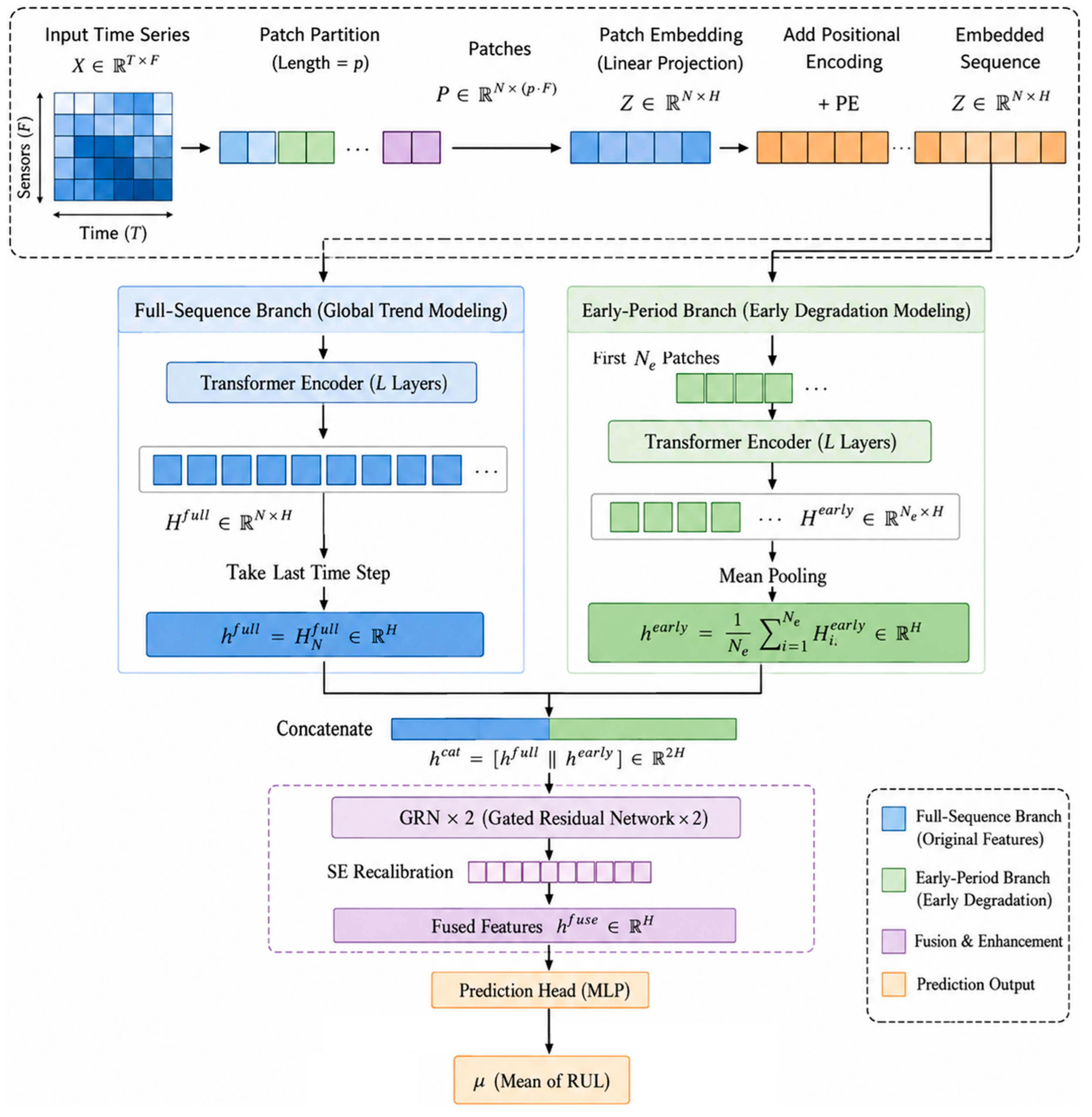
In contrast, the proposed method introduces a multi-view temporal perturbation learning framework built upon a dual-branch Transformer–GRN backbone. By jointly optimizing regression loss, multi-view consistency learning, and temporal ordering constraints, the proposed framework learns not only accurate degradation representations but also the structural relationships among different temporal observations. Consequently, the proposed method achieves the best overall performance across datasets with different degradation complexities. Specifically, when roll_k = 3, the proposed method obtains the lowest RMSE values of 13.44, 15.41, 13.80, and 16.63 on FD001, FD002, FD003, and FD004, respectively, demonstrating its strong capability in modeling degradation processes under both single/multiple operating conditions and single/multiple fault modes.

Besides prediction accuracy, predictive uncertainty is further evaluated through the uncertainty metric. As shown in Table 1, Table 2, Table 3 and Table 4, the proposed method consistently achieves lower uncertainty compared with most competing approaches. On FD001, the uncertainty decreases from 5.10 under roll_k = 1 to 4.15 under roll_k = 3. Similarly, on FD002, FD003, and FD004, uncertainty reaches 4.98, 3.76, and 5.18, respectively, when roll_k = 3. These results indicate that the proposed multi-view temporal perturbation strategy effectively reduces prediction dispersion caused by different temporal observations. By learning degradation-invariant representations across diverse temporal views, the model maintains stable prediction performance under different operating conditions and fault modes.

Reliability is further employed to evaluate the consistency between prediction confidence and actual prediction performance. The proposed method achieves the highest reliability values on the four datasets when roll_k = 3, reaching 0.85, 0.81, 0.81, and 0.79 on FD001, FD002, FD003, and FD004, respectively. Compared with Deep Quantile Regression, which explicitly models predictive uncertainty, the proposed framework achieves better reliability while maintaining competitive uncertainty estimation. These results demonstrate that the proposed multi-view learning strategy not only improves prediction accuracy but also provides better-calibrated confidence estimation for practical predictive maintenance applications.

The influence of different temporal perturbation magnitudes was investigated by varying the roll_k parameter. The experimental results show that increasing the perturbation range generally improves overall model performance. On FD001, FD002, FD003, and FD004, roll_k = 3 achieves the best comprehensive performance among different perturbation settings. Larger temporal perturbations expose the model to more diverse degradation observations, allowing it to capture invariant degradation characteristics across temporal views while reducing prediction variance. This advantage becomes more significant on FD002 and FD004, where multiple operating conditions introduce additional variations into degradation trajectories. The results demonstrate that the proposed temporal perturbation strategy is effective not only for relatively simple degradation scenarios but also for more challenging environments involving complex operating conditions and multiple fault modes.

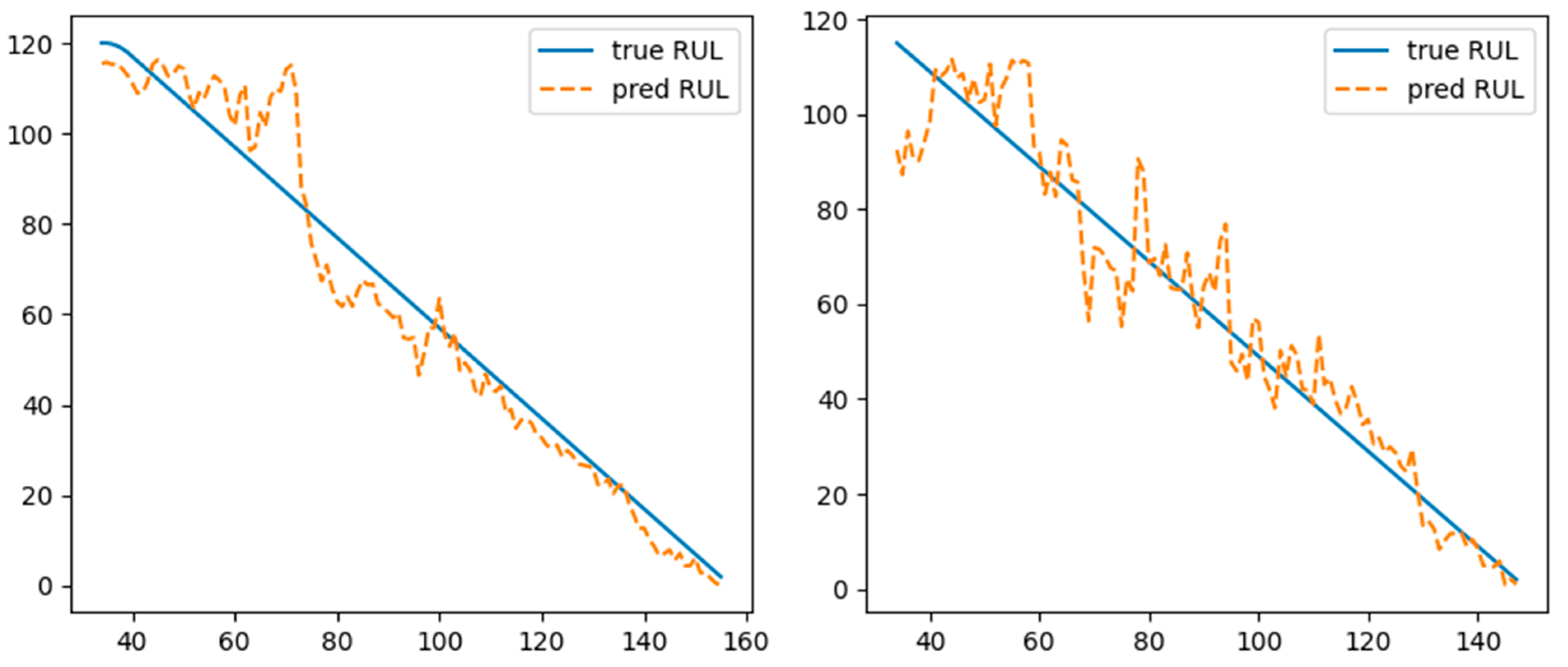
We present the prediction results of the two FD001 machines in the form of a line graph, as shown in Figure 2. It can be seen that the prediction results are basically close to the actual results. The experimental results demonstrate that the proposed multi-view temporal structure-aware learning framework effectively integrates multi-view temporal perturbation, consistency learning, and temporal ordering constraints into a unified optimization framework. By jointly improving prediction accuracy, reducing predictive uncertainty, and enhancing prediction reliability, the proposed method achieves robust and trustworthy Remaining Useful Life (RUL) prediction across the four C-MAPSS benchmark datasets with different levels of degradation complexity.

4.4. Framework Ablation

To further verify the contribution of each component mechanism proposed in this paper to the improvement in model performance, a framework ablation experiment is designed. In all experiments, the same data preprocessing method, dual-branch Transformer–GRN base prediction network, and training parameters are used, and only multi-view temporal perturbation, multi-view stability constraint, and temporal order constraint are gradually introduced to ensure the fairness of the experimental results. RUL prediction is performed using only the dual-branch Transformer–GRN base prediction network without introducing multi-view temporal perturbation or any additional constraints. This model is trained only with the original temporal window and uses mean square error as the optimization objective to evaluate the performance of the base prediction network. The multi-view temporal perturbation mechanism is introduced into the base prediction network, where training samples are constructed using both the original temporal window and its time offset windows before and after it; however, supervision learning still relies solely on predictions corresponding to the original view without introducing any additional structural constraints. This experiment aims to verify how much impact multi-view input has on learning ability for degraded features. On top of multi-view input, a multi-view stability constraint is added that guides models toward learning more stable degradation representations by minimizing statistical variance between predictions from different temporally perturbed views so as to reduce fluctuations in predictions caused by temporal perturbations. The further addition of a temporal order constraint explicitly constrains three temporally perturbed view predictions through a ranking loss satisfying the following:

$${\mu }_2<{\mu }_0<{\mu }_1,$$

so that models learn not only predictive errors but also time evolution laws during device degradation processes; this constitutes our proposed complete model.

Table 5. Results of frame ablation experiments.

Backbone	Multi-View	Consistency Loss	Ordering Loss	RMSE ↓	Uncertainty ↓	Reliability ↑
✓	×	×	×	15.08 ± 0.38	5.87 ± 0.2	0.66 ± 0.02
✓	✓	×	×	14.71 ± 0.28	5.12 ± 0.17	0.72 ± 0.01
✓	✓	✓	×	14.43 ± 0.36	4.63 ± 0.19	0.79 ± 0.02
✓	✓	✓	✓	13.44 ± 0.41	4.15 ± 0.14	0.85 ± 0.02

presents the experimental results for models under different component mechanisms.

As shown in Table 5, each component brings consistent improvements. Check marks (✓) in every line indicate that the current condition is included, while incorrect marks (×) indicate that the current condition is not included (The same applies below). The multi-view perturbation alone reduces RMSE from 15.08 to 14.71 and uncertainty from 5.87 to 5.12 and improves reliability from 0.66 to 0.72. Adding the consistency loss further enhances stability (uncertainty: 5.12 → 4.63). Finally, the ordering constraint incorporates the monotonic degradation prior, achieving the best overall performance (RMSE: 13.44; reliability: 0.85). These results demonstrate that the three mechanisms work synergistically, confirming the effectiveness of the proposed multi-view temporal structure-aware learning framework.

4.5. Network Ablation

In addition to verifying the effectiveness of each component mechanism in the multi-view learning framework, this paper further analyzes the contribution of each network structure in the basic prediction network to model performance. Under the premise of keeping the training strategy and loss function completely consistent, the dual-branch Transformer structure, gated residual network (GRN), and Squeeze-and-Excitation (SE) attention module are gradually introduced, respectively, and the prediction performance of models under different network structures is compared.

As shown in

Table 6. Results of network structure ablation experiment.

Dual Branch	GRN	SE	RMSE ↓	Uncertainty ↓	Reliability ↑
×	×	×	14.97 ± 0.42	5.33 ± 0.22	0.72 ± 0.03
✓	×	×	14.61 ± 0.37	5.08 ± 0.13	0.75 ± 0.02
✓	✓	×	14.12 ± 0.38	4.61 ± 0.17	0.80 ± 0.02
✓	✓	✓	13.44 ± 0.41	4.15 ± 0.14	0.85 ± 0.02

, each network component contributes to performance improvement. The dual-branch structure enables the model to capture both global and early-stage degradation information, reducing RMSE from 14.97 to 14.61. Adding a GRN further enhances feature fusion (RMSE: 14.61 → 14.12). The SE attention module provides additional improvement by recalibrating channel importance, achieving the best overall performance (RMSE: 13.44; reliability: 0.85).

4.6. Hyperparameter Sensitivity Analysis

To investigate the influence of key hyperparameters on the performance of the proposed framework, extensive sensitivity analyses were conducted on the FD001 dataset. The investigated parameters include the temporal perturbation magnitude k, the consistency loss weight λ1, the temporal ordering loss weight λ2, and the margin parameter m. The FD001 dataset was selected as the evaluation benchmark because it represents a relatively simple degradation scenario, allowing for the clearer observation of the effects caused by individual parameter variations.

It should be noted that all hyperparameters were determined according to their performance on the validation set rather than the test set. The test set was only used for the final evaluation after completing model selection. During sensitivity analysis, one parameter was varied while keeping other parameters fixed to their default values.

As shown in

Table 7. Sensitivity analysis of temporal perturbation magnitude k.

k	RMSE ↓	Uncertainty ↓	Reliability ↑
1	13.72 ± 0.33	5.10 ± 0.18	0.74 ± 0.02
2	13.83 ± 0.26	4.68 ± 0.21	0.78 ± 0.01
3	13.44 ± 0.41	4.15 ± 0.14	0.85 ± 0.02
4	13.61 ± 0.37	4.32 ± 0.17	0.83 ± 0.02
5	13.95 ± 0.45	4.56 ± 0.20	0.79 ± 0.03

, increasing k from 1 to 3 gradually improves the overall performance, indicating that moderate temporal perturbations provide more effective multi-view degradation information. However, excessively large perturbations (k = 4 or 5) slightly degrade performance because overly shifted temporal observations may introduce irrelevant variations. Therefore, k = 3 was selected as the optimal perturbation magnitude.

Table 8. Sensitivity analysis of temporal perturbation magnitude λ1.

λ1	RMSE ↓	Uncertainty ↓	Reliability ↑
0.01	13.91 ± 0.35	4.72 ± 0.19	0.78 ± 0.02
0.05	13.62 ± 0.32	4.39 ± 0.16	0.82 ± 0.02
0.10	13.44 ± 0.41	4.15 ± 0.14	0.85 ± 0.02
0.50	13.68 ± 0.38	4.36 ± 0.18	0.82 ± 0.03
1.00	14.05 ± 0.44	4.91 ± 0.23	0.76 ± 0.03

indicates that a moderate consistency constraint improves prediction stability and reliability. When λ1 is too small, the model cannot fully exploit multi-view consistency information. Conversely, an excessively large λ1 causes over-regularization and weakens regression optimization. Therefore, λ1 = 0.1 provides the best balance.

Similar observations can be found for λ2. We select an appropriate value for λ2 based on the ratio of λ1 to λ2. As shown in

Table 9. Sensitivity analysis of temporal perturbation magnitude λ1/λ2.

λ1/λ2	RMSE ↓	Uncertainty ↓	Reliability ↑
2.00	13.76 ± 0.36	4.51 ± 0.17	0.81 ± 0.02
1.00	13.57 ± 0.34	4.31 ± 0.15	0.83 ± 0.02
0.50	13.44 ± 0.41	4.15 ± 0.14	0.85 ± 0.02
0.20	13.59 ± 0.39	4.28 ± 0.17	0.83 ± 0.02

, increasing the ordering loss weight improves the reliability metric by enhancing degradation monotonicity. However, an excessively large value introduces strong ranking constraints and limits the flexibility of regression learning. The optimal value is obtained at λ2 = 0.2 (λ1 = 0.1 and λ1/λ2 = 0.5).

The margin parameter affects the strength of temporal ordering constraints. A small margin may provide insufficient degradation ordering supervision, while a very large margin makes the constraint excessively strict. As shown in

Table 10. Sensitivity analysis of temporal perturbation magnitude m.

m	RMSE ↓	Uncertainty ↓	Reliability ↑
0.1	13.65 ± 0.35	4.33 ± 0.15	0.83 ± 0.02
0.5	13.44 ± 0.41	4.15 ± 0.14	0.85 ± 0.02
1.0	13.52 ± 0.39	4.22 ± 0.16	0.84 ± 0.02
2.0	13.89 ± 0.47	4.68 ± 0.21	0.80 ± 0.03

, the model achieves the best performance when m = 0.5, which provides an appropriate balance between degradation ordering and regression accuracy.

5. Conclusions and Future Work

This paper addresses three issues in service prediction, namely sensitivity to temporal perturbations, insufficient predictive stability, and the lack of degradation structural constraints, by proposing a multi-view temporal structure learning framework. The framework first applies a patch partitioning strategy to transform multivariate time series into local semantic representations and then constructs a dual-branch Transformer–GRN predictive network to extract feature information from both the complete degradation process and its early-stage observations. A GRN combined with SE attention is further employed to enhance feature fusion. During training, a multi-view temporal perturbation strategy is introduced to generate multiple temporal observation views, together with multi-view stability and temporal ordering constraints, thereby improving robustness to temporal perturbations while maintaining prediction accuracy and degradation order consistency. The experimental results on the NASA C-MAPSS datasets demonstrate the effectiveness of the proposed framework. It achieves competitive or superior performance compared with the comparative methods in terms of prediction accuracy, temporal stability, and reliability. Ablation experiments on both the overall framework and network architecture further validate the effectiveness of the individual components, demonstrating that the proposed method can effectively exploit multi-view temporal information and prior knowledge of degradation structures to achieve more accurate, stable, and interpretable RUL predictions. From a practical PHM perspective, improving prediction stability across adjacent observation windows is important because excessive RUL fluctuations may lead to inappropriate maintenance decisions. Therefore, the proposed framework provides benefits beyond numerical prediction accuracy by improving the reliability and consistency of RUL estimates, which is valuable for practical maintenance decision-making.

Although NASA C-MAPSS provides a standardized benchmark for evaluating RUL prediction algorithms, it is still a simulated dataset and may not fully capture the complex degradation patterns, operational variations, and measurement uncertainties encountered in real industrial environments. Therefore, although the experimental results demonstrate the effectiveness and robustness of the proposed framework under different degradation scenarios, its generalization capability in practical industrial applications remains to be further validated. Future research will focus on evaluating the proposed framework using real-world industrial degradation datasets collected from practical equipment and investigating its adaptability to more diverse operating conditions, degradation patterns, and fault modes.