RAPC-Net: Residual-Aware Physical Consistency Network for Multi-Appliance NILM

Abstract

Non-intrusive load monitoring (NILM) aims to estimate appliance-level power consumption from aggregate household measurements and provides an effective solution for fine-grained energy management. However, multi-appliance NILM remains challenging because the measured aggregate power generally contains unobserved household loads, jointly predicted appliance powers may violate basic physical relationships, and heterogeneous appliance activation patterns can lead to imbalanced optimization. To address these issues, this paper proposes a Residual-Aware Physical Consistency Network (RAPC-Net) for multi-appliance NILM. RAPC-Net jointly estimates multiple target appliances and the remaining household consumption through a shared temporal encoder, a multi-appliance prediction branch, and a residual-load prediction branch. Two watt-space physical consistency constraints are incorporated into the learning objective. The aggregate reconstruction constraint encourages the target-appliance predictions and the predicted residual load to jointly reconstruct the measured aggregate power, while the overestimation constraint suppresses physically infeasible predictions in which the sum of the predicted target-appliance powers exceeds the aggregate measurement. In addition, an automatic appliance-aware weighting strategy is developed based on appliance activation statistics to balance the contributions of different appliances and emphasize active samples without manually assigning appliance-specific loss coefficients. Experiments on the REFIT dataset, including an expanded ablation study and two house-independent comparisons, are conducted to evaluate the contributions of residual-load modeling, physical consistency constraints, and appliance-aware weighting. In the primary house-independent comparison, RAPC-Net achieves a Target-sum MAE of $85.97\pm 15.45$ W, which is close to the best competing result of $83.59\pm 3.71$ W, while reducing the Over-ratio to $0.025\pm 0.020\%$ and the violation energy to $9.10\pm 5.47$ Wh. Under an additional household partition, RAPC-Net maintains a Target-sum MAE of $127.29\pm 7.05$ W and achieves an Over-ratio of $0.019\pm 0.011\%$. These results indicate that RAPC-Net improves the physical feasibility of joint multi-appliance predictions while maintaining comparable target-sum estimation accuracy.

1. Introduction

The increasing penetration of smart meters and advanced metering infrastructure has provided large amounts of household electricity data and created new opportunities for demand-side management, energy-efficiency improvement, and intelligent residential energy services. Non-intrusive load monitoring (NILM), originally introduced to infer appliance-level consumption from measurements collected at a single monitoring point [1], provides a cost-effective alternative to installing dedicated sensors on individual electrical devices. By decomposing aggregate household power into appliance-level consumption, NILM can support detailed energy feedback, demand response, load scheduling, and residential energy management. Owing to these practical benefits, NILM has received extensive research attention, and recent reviews have systematically summarized its methodological development, application scenarios, and remaining challenges toward practical deployment [2,3]. More broadly, related data-driven representation learning techniques have also been extensively investigated in intelligent industrial monitoring and fault diagnosis, including nonlinear process monitoring, quality-relevant diagnosis, and learning under limited or imbalanced labeled data [4,5,6,7].

Traditional NILM methods mainly rely on manually designed electrical signatures, event-based disaggregation, hidden Markov models, and related probabilistic techniques. Cominola et al. [8] proposed a hybrid signature-based iterative disaggregation algorithm, while Kumar and Abhyankar [9] developed a time-efficient factorial hidden Markov model for load disaggregation. Although these approaches are relatively interpretable, their performance can be sensitive to handcrafted features and prior assumptions, particularly when different appliances exhibit similar power levels, transient operating behaviors, or multiple operating states. With the development of deep learning, data-driven NILM methods have increasingly replaced manual feature engineering by learning discriminative representations directly from aggregate load sequences. Kelly and Knottenbelt [10] introduced deep neural networks into energy disaggregation, indicating the potential of neural representation learning for NILM. Feng et al. [11] developed a multichannel spatio-temporal feature fusion method to capture complementary appliance characteristics, while Yang et al. [12] employed temporal convolutional networks to model temporal dependencies in aggregate load signals. Zhang et al. [13] subsequently proposed sequence-to-point learning, which maps an aggregate power window to the target-appliance power at its center point and has become a widely adopted NILM formulation because of its effective feature utilization and relatively simple inference procedure. The sequence-to-point formulation is also adopted in the present work.

Recent studies have further focused on strengthening the temporal representation capability of NILM models. Zhang et al. [14] introduced dilated and residual convolutional structures to enlarge the receptive field and capture temporal information over different time scales. Li et al. [15] proposed TF-LGNet, which combines time-frequency representation with multi-scale local feature extraction and global feature modeling to characterize the non-stationary and multi-scale characteristics of aggregate load signals. Geng et al. [16] developed MSDCANet to enhance multi-scale feature extraction and discriminative feature selection through a dual-channel convolutional attention architecture. Piccialli and Sudoso [17] introduced an attention-based deep neural network to emphasize informative temporal features, while Sykiotis et al. [18] developed the ELECTRIcity Transformer to model long-range dependencies in NILM signals. More recently, Jiang et al. [19] proposed ConvTransNILM, which combines convolutional feature extraction with Transformer-based global dependency modeling to improve disaggregation performance while controlling computational complexity. Collectively, these studies suggest that multi-scale temporal modeling and global dependency learning are promising approaches for appliance-level power estimation.

In addition to feature representation, model generalization across appliances and households remains an important issue in NILM. Li et al. [20] proposed an adaptive fusion feature transfer learning method that integrates multi-branch feature extraction, adaptive feature fusion, and attention-based transfer to improve generalization across different NILM domains. Similar domain variation problems also arise in other smart-building sensing applications. Yang et al. [21] systematically investigated deep learning and transfer learning for device-free human activity recognition and highlighted the importance of transferable representations under limited labeled data. Nevertheless, most conventional NILM frameworks still train an independent model for each target appliance, which may lead to repeated feature extraction and increasing computational and storage costs as the number of monitored appliances grows.

Another important research direction is multi-appliance NILM, in which several appliances are estimated simultaneously using a unified model. Compared with training an independent network for each appliance, multi-appliance architectures can share feature representations, reduce model redundancy, and potentially exploit relationships among different appliance loads. Xia et al. [22] developed a composite deep long short-term memory network with an encoder–separation–decoder structure to map an aggregate power sequence to multiple appliance-level outputs. Li et al. [23] further proposed an adaptive one-to-many NILM framework combined with transfer learning, allowing a single model to estimate multiple appliances while improving transferability across appliances and data domains. Xiong et al. [24] introduced MATNilm, a multi-appliance-task architecture with shared hierarchical structures and a two-dimensional attention mechanism for joint appliance-related regression and classification under limited labeled data. Li et al. [25] proposed MA-NILM, which explicitly separates common representations shared among appliances from appliance-specific individual features and subsequently combines them through attention-based feature adjustment for simultaneous multi-appliance disaggregation. These studies indicate that shared representation learning and joint prediction constitute a promising direction for scalable NILM.

Beyond improving prediction accuracy through increasingly sophisticated network architectures, recent research in intelligent modeling and control has emphasized that purely data-driven predictions should also be compatible with the known physical characteristics of the underlying system. Song et al. [26] discussed physically interpretable and trustworthy learning by incorporating physical laws, system dynamics, and explicit constraints into data-driven models. Li et al. [27] developed a learning-based framework for remaining useful life prediction, while Liu et al. [28] introduced physics-informed reduced-order modeling for real-time control of soft actuators. These studies illustrate the potential value of combining data-driven learning with physically meaningful constraints. This perspective is particularly relevant to multi-appliance NILM because the predicted powers of different appliances are not completely independent. Their joint estimation is inherently constrained by the measured aggregate household power.

Nevertheless, several issues remain insufficiently addressed in existing multi-appliance NILM approaches. First, most methods directly estimate a predefined set of target appliances while treating the remaining household consumption only implicitly. In practical residential measurements, however, the aggregate power generally contains contributions from numerous unobserved appliances, background loads, standby consumption, and measurement uncertainty. Consequently, when only a subset of household appliances is selected as prediction targets, the measured aggregate signal cannot generally be interpreted as the exact sum of these target appliances. Neglecting this unobserved component may result in part of the remaining household consumption being attributed to the selected appliances, thereby affecting joint multi-appliance estimation.

Second, conventional appliance-wise regression objectives do not explicitly guarantee physical compatibility between jointly predicted appliance loads and the measured aggregate power. When multiple appliance outputs are optimized primarily through independent regression losses, their predicted power sum may exceed the aggregate measurement at some time steps. Such predictions can still yield acceptable appliance-level errors while violating the basic physical relationship between the aggregate signal and its constituent loads. Incorporating aggregate-level information into model optimization is therefore desirable. However, directly forcing the sum of only the selected target appliances to equal the measured aggregate power is also inappropriate because non-target consumption is generally present. Effective physical consistency learning should therefore simultaneously account for unobserved household loads and constrain physically implausible target-appliance predictions.

Third, multi-appliance learning is affected by considerable heterogeneity in appliance activation patterns. Frequently operating appliances, such as refrigerators, provide a relatively large number of active samples, whereas kettles and microwaves typically exhibit sparse and short-duration activations. Washing machines and dishwashers may additionally contain long-duration and multi-stage operating cycles. Uniformly averaging the losses of different appliances can therefore provide imbalanced supervision, causing frequently active or high-magnitude loads to dominate optimization while sparse appliance activations receive insufficient emphasis. Although manually assigning appliance-specific loss coefficients can alleviate this problem, such coefficients introduce additional hyperparameters and may require retuning when the appliance combination or dataset changes.

For downstream energy-management applications, the physical consistency of disaggregated loads is important because appliance-level estimates may be used as inputs to demand-response, load-scheduling, and energy-balance calculations. If the sum of the estimated appliance loads exceeds the measured aggregate power, the resulting allocation is physically infeasible and may distort the estimation of controllable demand. Related energy-management studies indicate that electrical measurements and power-balance information need to be connected to explicit control strategies and technical-economic indicators when assessing operational and economic benefits [29]. The present study focuses on improving the physical consistency of multi-appliance disaggregation and does not directly implement a downstream controller or evaluate changes in scheduling decisions or operating costs.

To address these issues, this paper proposes a Residual-Aware Physical Consistency Network (RAPC-Net) for multi-appliance NILM. RAPC-Net integrates residual-load modeling, watt-space physical consistency constraints, and automatic appliance-aware weighting within a unified multi-appliance prediction framework. The main contributions of this work are summarized as follows:

• A residual-aware multi-appliance NILM formulation is proposed, in which the selected target-appliance loads and the remaining household consumption are explicitly modeled through separate prediction branches. This formulation avoids forcing a limited set of target appliances to account for the entire aggregate household power.
• Two watt-space physical consistency constraints are incorporated into the learning objective. The aggregate reconstruction constraint exploits the relationship among the target-appliance predictions, residual-load prediction, and measured aggregate power, while the overestimation constraint suppresses physically infeasible predictions in which the predicted target-appliance sum exceeds the aggregate measurement.
• An automatic appliance-aware weighting strategy is developed to address heterogeneous appliance activation patterns. Its weighting factors are automatically derived from training-set statistics to balance the contributions of different appliances and emphasize active samples without manually specifying appliance-level loss coefficients.
• Experiments on the REFIT dataset are conducted through an expanded ablation study and two house-independent comparisons with representative multi-appliance NILM methods. The results suggest that residual-load modeling, physical consistency constraints, and appliance-aware weighting provide complementary contributions to joint multi-appliance estimation.

The remainder of this paper is organized as follows. Section 2 formulates the residual-aware multi-appliance NILM problem. Section 3 presents the proposed RAPC-Net, including the shared temporal feature encoder, residual-aware prediction framework, automatic appliance-aware weighting strategy, and physical consistency constraints. Section 4 describes the experimental setup, parameter sensitivity analysis, ablation study, house-independent comparisons, and computational complexity analysis. Finally, Section 5 concludes this paper.

2. Problem Formulation

NILM aims to estimate the power consumption of individual appliances from the aggregate household power signal. Let $x_t\in \mathbb{R}$ denote the aggregate power reading at time step t, and let $y_t={[y_t^1,y_t^2,\dots ,y_t^K]}^{\top }\in {\mathbb{R}}^K$ denote the power consumption vector of K target appliances, where $y_t^k$ represents the power consumption of the k-th appliance. In this study, the aggregate household power is modeled as the combination of the selected target-appliance loads and a residual component:

$$x_t\approx {\displaystyle \sum _{k=1}^K}{y}_t^k+r_t,$$

(1)

where $r_t$ denotes the non-negative portion of household consumption that is not attributed to the selected target appliances. The approximate relationship accounts for the presence of unobserved loads and possible measurement discrepancies between the aggregate and appliance-level channels.

Following the sequence-to-point NILM setting, a fixed-length aggregate power window centered at time step t is used as the model input:

$$x_t={[x_{t-L},\dots ,x_t,\dots ,x_{t+L}]}^{\top }\in {\mathbb{R}}^W,$$

(2)

where $W=2L+1$ is the window length. The objective is to learn a mapping function $f_{\theta }(·)$ parameterized by $\theta$:

$$({\widehat{y}}_t,{\widehat{r}}_t)=f_{\theta }\left(x_t\right),$$

(3)

where ${\widehat{y}}_t={[{\widehat{y}}_t^1,{\widehat{y}}_t^2,\dots ,{\widehat{y}}_t^K]}^{\top }$ is the predicted power vector of the target appliances, and ${\widehat{r}}_t$ is the predicted residual load.

Unlike single-appliance NILM, multi-appliance disaggregation requires the simultaneous estimation of multiple appliance loads. This setting is challenging because different appliances may exhibit heterogeneous activation frequencies, power magnitudes, operating durations, and temporal patterns. In addition, the jointly predicted target-appliance loads should remain physically compatible with the observed aggregate power. Therefore, the predictions are encouraged to satisfy the following soft physical relationship:

$${\displaystyle \sum _{k=1}^K}{\widehat{y}}_t^k+{\widehat{r}}_t\approx x_t,$$

(4)

where ${\widehat{r}}_t$ represents the predicted non-negative household consumption that is not attributed to the selected target appliances. Because the aggregate and appliance-level channels are measured separately and the selected target appliances do not represent all household loads, Equation (4) is treated as a soft reconstruction relationship rather than an exact sample-wise identity.

For model training, the residual label is defined as the non-negative difference between the aggregate power and the sum of the measured target-appliance powers:

$$r_t=\max \left(x_t-{\displaystyle \sum _{k=1}^K}{y}_t^k,0\right).$$

(5)

The aggregate and appliance-level channels are first aligned to a common sampling grid. Nevertheless, small inconsistencies may remain because of asynchronous measurements, timing jitter, meter calibration errors, or other measurement noise. Consequently, $x_t<{\sum }_{k=1}^K{y}_t^k$ may occur at some time steps. The max operator prevents such discrepancies from being interpreted as physically negative residual consumption while preserving the original appliance-level regression targets. For samples at which the residual label is clipped to zero, exact additivity is not imposed on the training labels. Instead, the remaining discrepancy is retained in the aggregate reconstruction loss, which is evaluated using the original aggregate power measurement. Therefore, $r_t$ is interpreted as a non-negative auxiliary target for residual-load learning rather than an exact algebraic remainder.

Given a training set

$$D={\left\{(x_t,y_t,r_t,x_t)\right\}}_{t=1}^N,$$

(6)

the learning objective is to estimate the power consumption of all target appliances while maintaining consistency among the aggregate power, target-appliance predictions, and residual-load prediction. Accordingly, the proposed model is optimized by jointly considering appliance-level regression accuracy, residual-load estimation, and aggregate-level physical consistency.

3. Proposed Method

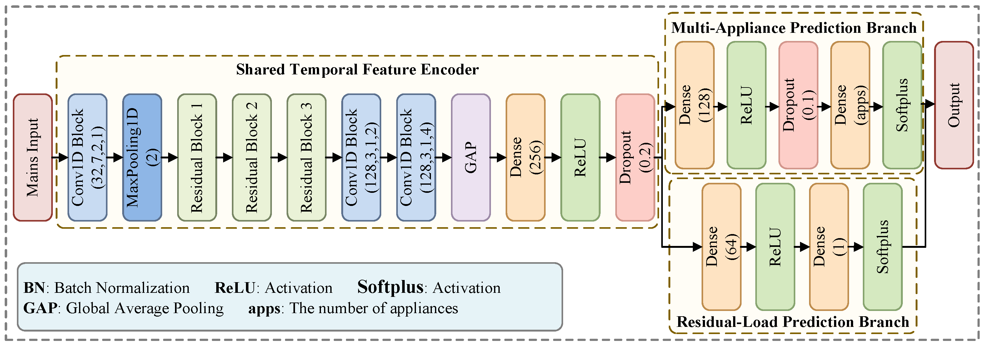
This section presents the proposed Residual-Aware Physical Consistency Network (RAPC-Net) for multi-appliance NILM. As illustrated in Figure 1, RAPC-Net consists of a shared temporal feature encoder, a multi-appliance prediction branch, and a residual-load prediction branch. Automatic appliance-aware weighting is used to account for heterogeneous appliance activation patterns, while physical consistency constraints are incorporated into the training objective to improve the compatibility between the jointly predicted appliance powers and the measured aggregate power.

3.1. Shared Temporal Feature Encoder

Given an aggregate power window $x_t$, the shared temporal feature encoder extracts a compact representation containing local appliance signatures and temporal contextual information. The encoder comprises a convolutional stem, three residual blocks, two dilated convolutional blocks, and a global feature aggregation module, as shown in Figure 1.

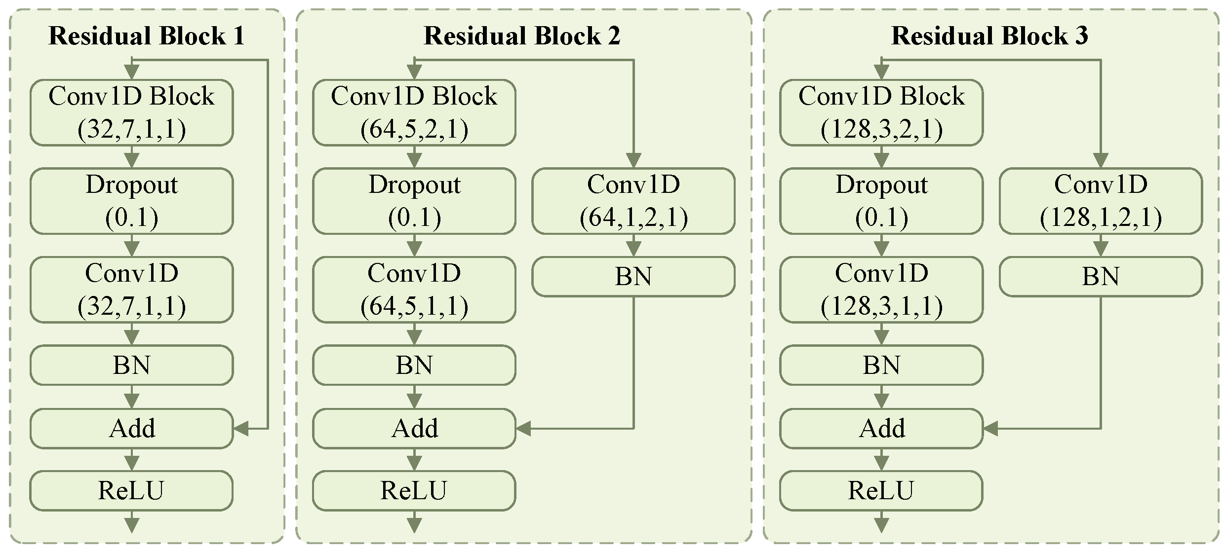
The convolutional stem performs initial feature extraction and temporal downsampling. The subsequent residual blocks gradually increase the feature dimension while reducing the temporal resolution. Residual connections are used to facilitate gradient propagation and retain information from preceding layers. The internal structures and parameter configurations of the three residual blocks are illustrated in Figure 2.

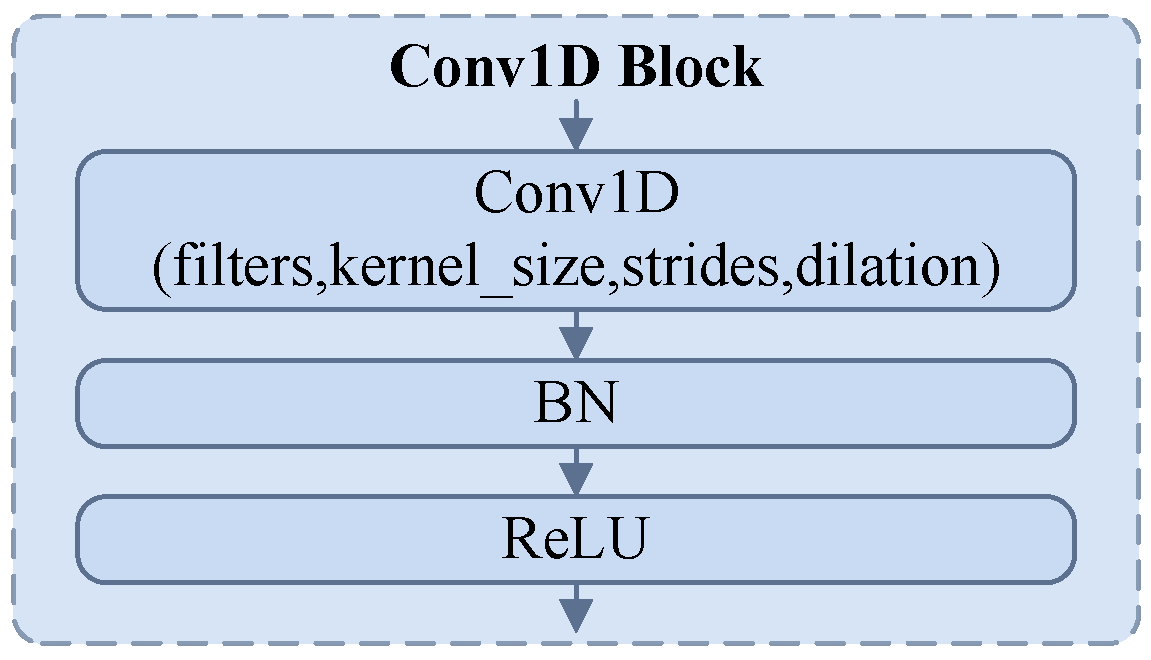
The dilated convolutional blocks enlarge the receptive field without proportionally increasing the number of convolutional parameters, allowing temporal information at different scales to be incorporated into the learned representation. The internal structure of the Conv1D block used in the temporal feature encoder is shown in Figure 3.

The output of the shared temporal feature encoder is denoted by

$$h_t=F_{\mathrm{enc}}\left(x_t\right),$$

(7)

where $F_{\mathrm{enc}}(·)$ denotes the shared temporal feature encoder, and $h_t$ is the learned feature representation provided to the two prediction branches.

3.2. Residual-Aware Multi-Output Prediction

Conventional multi-output NILM models generally estimate the power consumption of a predefined set of target appliances without explicitly representing unobserved household loads. However, the aggregate power may also contain contributions from non-target appliances, background loads, standby consumption, and measurement discrepancies. Directly forcing the sum of the target-appliance predictions to match the aggregate measurement may therefore assign part of the unobserved consumption to the selected appliances.

To account for this component, RAPC-Net introduces a residual-load prediction branch in addition to the multi-appliance prediction branch. Based on the shared representation $h_t$, the two branches jointly estimate

$${\widehat{y}}_t={\left[{\widehat{y}}_t^1,{\widehat{y}}_t^2,\dots ,{\widehat{y}}_t^K\right]}^{\top },{\widehat{r}}_t,$$

(8)

where ${\widehat{y}}_t$ denotes the predicted power vector of the K target appliances, and ${\widehat{r}}_t$ denotes the predicted residual load.

The multi-appliance branch jointly estimates the power consumption of all selected target appliances from the shared temporal representation. This shared structure allows common temporal information to be used across the appliance outputs while retaining an individual output for each target appliance. The residual branch estimates the non-negative portion of household consumption that is not attributed to the selected target appliances. Both branches use non-negative output activations to produce non-negative power estimates.

The residual target $r_t$ is calculated using Equation (5). Explicit residual-load modeling is intended to represent the unobserved component of the aggregate measurement, thereby reducing the need for the selected target-appliance outputs to account for the entire household demand.

3.3. Automatic Appliance-Aware Weighting

Multi-appliance NILM is characterized by considerable heterogeneity across appliances. Frequently operating appliances provide relatively large numbers of active training samples, whereas sparsely activated appliances contribute relatively few non-zero observations. Furthermore, appliance power magnitudes can differ substantially. Directly averaging the losses of all appliances may therefore result in imbalanced contributions to model optimization, with frequently active or high-power appliances contributing more strongly than sparsely activated appliances.

To address this issue, an automatic appliance-aware weighting (AAW) strategy is introduced. Let ${\rho }_k$ denote the activation ratio of the k-th appliance in the training set. It is calculated as

$${\rho }_k={\displaystyle \frac{1}{N}}{\displaystyle \sum _{t=1}^N}\mathbb{I}\left(y_t^k\ge {\delta }_k\right),$$

(9)

where ${\delta }_k$ is the activation threshold of the k-th appliance, and $\mathbb{I}(·)$ denotes the indicator function.

An appliance-level base weight is first derived from the activation ratio:

$${\alpha }_k=\mathrm{clip}\left[{\left({\displaystyle \frac{{\rho }_{\mathrm{ref}}}{{\rho }_k+ϵ}}\right)}^{1/4},{\alpha }_{\min },{\alpha }_{\max }\right],$$

(10)

where ${\rho }_{\mathrm{ref}}$ is the reference activation ratio, $ϵ$ is a small positive constant used for numerical stability, and $\mathrm{clip}(·)$ restricts the weight to the interval $[{\alpha }_{\min },{\alpha }_{\max }]$. According to this formulation, an appliance with a lower activation ratio generally receives a larger base weight, subject to the specified clipping bounds.

To further increase the contribution of active samples, an additional ON-state weighting factor is calculated as

$${\beta }_k=\mathrm{clip}\left[\sqrt{{\displaystyle \frac{1-{\rho }_k}{{\rho }_k+ϵ}}},{\beta }_{\min },{\beta }_{\max }\right].$$

(11)

Let $m_t^k\in \{0,1\}$ denote the activation-state indicator of appliance k at time step t:

$$m_t^k=\mathbb{I}\left(y_t^k\ge {\delta }_k\right).$$

(12)

The resulting sample-level weight is defined as

$$w_t^k={\alpha }_k\left(1+{\beta }_k{m}_t^k\right).$$

(13)

Accordingly, the weight of an OFF-state sample is ${\alpha }_k$, whereas the weight of an ON-state sample is ${\alpha }_k(1+{\beta }_k)$. Thus, ${\alpha }_k$ adjusts the overall contribution of each appliance according to its activation ratio, while ${\beta }_k$ provides additional emphasis to its active samples.

The term ”automatic” in AAW does not imply that the weighting strategy is free of global hyperparameters. Instead, it indicates that the appliance-specific values of ${\alpha }_k$ and ${\beta }_k$ are automatically calculated from the activation statistics of the training data rather than manually assigned to individual appliances. Appliances with different ON-state ratios therefore receive different weights, whereas the same global clipping bounds are applied uniformly to all appliances. No appliance-dependent weighting coefficients are separately selected according to validation or test performance. The clipping bounds act as global regularization parameters that prevent excessively large weights for highly sparse appliances. Their influence is examined through the sensitivity analysis in Section 4.3.

The appliance-level regression loss is then formulated as

$$L_{\mathrm{power}}={\displaystyle \frac{1}{NK}}{\displaystyle \sum _{t=1}^N}{\displaystyle \sum _{k=1}^K}{w}_t^k{\mathsf{\ell }}_{\mathrm{H}}\left(y_t^k,{\widehat{y}}_t^k\right),$$

(14)

where ${\mathsf{\ell }}_{\mathrm{H}}(·)$ denotes the Huber loss with $\delta =1$.

3.4. Physical Consistency Constraints

Although the appliance and residual branches are directly supervised, their regression losses alone do not guarantee that the combined predictions are physically compatible with the measured aggregate power. To incorporate aggregate-level information into model optimization, two watt-space physical consistency constraints are introduced.

First, the reconstructed aggregate power is defined as the sum of the predicted target-appliance powers and the predicted residual load. The aggregate reconstruction loss is given by

$$L_{\mathrm{agg}}={\displaystyle \frac{1}{N}}{\displaystyle \sum _{t=1}^N}\left|x_t-\left({\displaystyle \sum _{k=1}^K}{\widehat{y}}_t^k+{\widehat{r}}_t\right)\right|.$$

(15)

This term penalizes the mismatch between the measured aggregate power and the power reconstructed from the two prediction branches.

Second, because the predicted target-appliance consumption should not exceed the measured aggregate power, an overestimation loss is introduced:

$$L_{\mathrm{over}}={\displaystyle \frac{1}{N}}{\displaystyle \sum _{t=1}^N}\mathrm{ReLU}\left({\displaystyle \sum _{k=1}^K}{\widehat{y}}_t^k-x_t\right).$$

(16)

Unlike a strict equality constraint imposed only on the target appliances, this formulation retains the contribution of unobserved household loads through the residual branch while penalizing target-appliance predictions whose sum exceeds the measured aggregate power.

Although $L_{\mathrm{agg}}$ and $L_{\mathrm{over}}$ are both related to aggregate-power consistency, they impose different constraints. To clarify their respective roles, the aggregate reconstruction error can be written as

$$e_t^{\mathrm{agg}}=x_t-{\displaystyle \sum _{k=1}^K}{\widehat{y}}_t^k-{\widehat{r}}_t.$$

(17)

The aggregate reconstruction loss penalizes both positive and negative reconstruction errors. It therefore produces a gradient when the reconstructed power is either lower or higher than the measured aggregate power. Because both prediction branches contribute to the reconstruction, the gradient of $L_{\mathrm{agg}}$ is propagated to the appliance and residual outputs.

In contrast, the target-appliance overestimation error is defined as

$$e_t^{\mathrm{over}}=\max \left({\displaystyle \sum _{k=1}^K}{\widehat{y}}_t^k-x_t,0\right).$$

(18)

$L_{\mathrm{over}}$ becomes active only when the sum of the predicted target-appliance powers exceeds the measured aggregate power. Because ${\widehat{r}}_t$ is constrained to be non-negative, reducing the residual prediction cannot correct a violation for which ${\sum }_k{\widehat{y}}_t^k>x_t$. Therefore, $L_{\mathrm{over}}$ directly penalizes the appliance outputs in this infeasible region and produces no direct gradient with respect to the residual output.

The interaction between the two physical consistency losses depends on the prediction region. When ${\sum }_k{\widehat{y}}_t^k+{\widehat{r}}_t<x_t$, only $L_{\mathrm{agg}}$ encourages an increase in the reconstructed power, while $L_{\mathrm{over}}$ remains inactive. When ${\sum }_k{\widehat{y}}_t^k\le x_t$ but ${\sum }_k{\widehat{y}}_t^k+{\widehat{r}}_t>x_t$, $L_{\mathrm{agg}}$ penalizes the reconstruction mismatch through both prediction branches, whereas $L_{\mathrm{over}}$ remains inactive because the predicted target-appliance sum does not exceed the aggregate measurement. When ${\sum }_k{\widehat{y}}_t^k>x_t$, both losses penalize the appliance outputs. In this region, $L_{\mathrm{over}}$ provides an additional one-sided gradient that cannot be eliminated by adjusting the non-negative residual output.

Meanwhile, the residual regression loss anchors the residual prediction to the auxiliary residual label defined in Equation (5). This supervision limits the extent to which the residual branch can absorb the aggregate reconstruction error. Depending on whether ${\widehat{r}}_t$ is above or below $r_t$, the residual-side gradient of $L_{\mathrm{res}}$ may reinforce or oppose that of $L_{\mathrm{agg}}$. Their relative contributions are controlled by ${\lambda }_{\mathrm{res}}$ and ${\lambda }_{\mathrm{agg}}$.

Thus, the three losses have distinct roles: $L_{\mathrm{agg}}$ penalizes household-level reconstruction errors over the full prediction range, $L_{\mathrm{over}}$ directly penalizes physically infeasible target-appliance sums, and $L_{\mathrm{res}}$ supervises the residual-load output. The influence of their relative weights is examined in Section 4.3.

3.5. Joint Optimization Objective

The residual branch is trained using the Huber loss between the auxiliary residual label $r_t$ and its prediction ${\widehat{r}}_t$:

$$L_{\mathrm{res}}={\displaystyle \frac{1}{N}}{\displaystyle \sum _{t=1}^N}{\mathsf{\ell }}_{\mathrm{H}}\left(r_t,{\widehat{r}}_t\right).$$

(19)

The complete training objective is formulated as

$$L={\lambda }_{\mathrm{power}}{L}_{\mathrm{power}}+{\lambda }_{\mathrm{res}}{L}_{\mathrm{res}}+{\lambda }_{\mathrm{agg}}{L}_{\mathrm{agg}}+{\lambda }_{\mathrm{over}}{L}_{\mathrm{over}},$$

(20)

where ${\lambda }_{\mathrm{power}}$, ${\lambda }_{\mathrm{res}}$, ${\lambda }_{\mathrm{agg}}$, and ${\lambda }_{\mathrm{over}}$ control the contributions of appliance-level regression, residual-load estimation, aggregate reconstruction, and target-appliance overestimation suppression, respectively.

The four loss terms provide different forms of supervision. Specifically, $L_{\mathrm{power}}$ directly supervises appliance-level power estimation, $L_{\mathrm{res}}$ supervises the residual-load output, $L_{\mathrm{agg}}$ penalizes bidirectional household-level reconstruction errors, and $L_{\mathrm{over}}$ imposes a one-sided penalty on physically infeasible target-appliance predictions. Their coefficients are shared global hyperparameters rather than appliance-specific values. The influence of these coefficients is evaluated through the sensitivity analysis in Section 4.3, based on which the final values used in the subsequent experiments are selected.

Through this joint objective, RAPC-Net is designed to learn shared temporal representations, estimate the selected appliance loads and the remaining household consumption, account for heterogeneous appliance activation patterns, and improve consistency with the measured aggregate signal.

4. Experiments

4.1. Dataset and Experimental Setup

The experiments are conducted on the REFIT dataset [30]. Five target appliances are considered: fridge, washing machine, dishwasher, microwave, and kettle. Their ON-state thresholds are listed in

Table 1. Appliance-specific ON-state thresholds.

Appliance	Threshold (W)
Fridge	50
Washing machine	20
Dishwasher	10
Microwave	200
Kettle	2000

. These thresholds are used only to calculate the F1-score and the activation statistics required by AAW; they are not used to modify the appliance power regression targets.

Table 2. Household and temporal partitions used in the experiments.

Experimental Setting	Data Role	House	Time Period
Sensitivity and Ablation	Training	House 9	1 September 2014 to 24 September 2014
	Validation	House 9	25 September 2014 to 30 September 2014
	Testing (ablation only)	House 9	12 April 2015 to 16 April 2015
Comparison Case 1	Training	House 2	1 September 2014 to 30 September 2014
		House 3	1 November 2014 to 30 November 2014
		House 5	1 October 2014 to 31 October 2014
	Validation	House 9	1 December 2014 to 21 December 2014
	Testing	House 20	1 January 2015 to 10 January 2015
Comparison Case 2	Training	House 3	1 November 2014 to 30 November 2014
		House 9	1 December 2014 to 30 December 2014
		House 20	1 January 2015 to 30 January 2015
	Validation	House 2	1 September 2014 to 20 September 2014
	Testing	House 5	1 October 2014 to 10 October 2014

summarizes the fixed household and temporal partitions used for training, validation, and testing. For the sensitivity and ablation experiments, the training and validation periods are chronologically separated within House 9. The test period is used only for the final ablation evaluation and is not involved in hyperparameter selection. In each comparison case, the validation and test households are excluded from the corresponding training set, thereby providing household-independent model selection and evaluation.

The aggregate and appliance-level signals are uniformly resampled at 8 s. Samples containing missing or invalid values are excluded, and the resulting discontinuities are treated as boundaries between independent continuous segments. The household and temporal partitions in Table 2 are defined before sliding-window generation. Each partition is then independently divided into input windows of length $W=599$ with a stride of one sample, and the appliance powers at the center point are used as prediction targets. Windows are not allowed to cross household, temporal-partition, or discontinuity boundaries. Because each window requires 299 context samples on either side of its center, boundary samples that cannot form a complete window are excluded. Thus, no raw samples are shared among the training, validation, and test windows. All compared methods use the same preprocessing, data partitions, window construction, and target definition.

The uniformly resampled REFIT data provide a standardized setting for algorithm-level evaluation but do not reproduce the complete acquisition chain of a practical NILM system. In real deployments, sensor noise, limited measurement accuracy, timestamp misalignment, missing measurements, and communication interruptions may distort appliance signatures or disrupt short-duration events. The reliability of data-driven electrical monitoring therefore depends on both the learning model and the quality and integration of the measurement chain, including sensing, synchronization, data transmission, preprocessing, and inference [31]. Accordingly, the present results should be interpreted as an evaluation on preprocessed benchmark data rather than validation of a complete physical acquisition system. Evaluation under different sensor accuracies, asynchronous measurements, communication losses, and resource-constrained embedded platforms is left for future work.

Adam is used with an initial learning rate of $3\times {10}^{-4}$, a batch size of 128, and a maximum of 20 training epochs. Early stopping monitors the validation loss with a patience of five epochs, and the model with the lowest validation loss is retained. The learning rate is reduced by a factor of 0.5 after three consecutive epochs without improvement in validation loss, with a minimum value of ${10}^{-6}$.

4.2. Evaluation Metrics

Performance is evaluated from three complementary aspects: appliance-level disaggregation accuracy, joint target-appliance estimation accuracy, and physical feasibility. MAE, RMSE, SAE, and F1-score evaluate appliance-level performance; Target-sum MAE evaluates the joint estimation of all target appliances; and Over-ratio and violation energy quantify the frequency and cumulative magnitude of aggregate-power violations, respectively.

For appliance k, the mean absolute error (MAE) is defined as

$${\mathrm{MAE}}_k={\displaystyle \frac{1}{N}}{\displaystyle \sum _{t=1}^N}\left|y_t^k-{\widehat{y}}_t^k\right|.$$

(21)

Here, $y_t^k$ and ${\widehat{y}}_t^k$ denote the ground-truth and predicted power consumption of the k-th appliance at time step t, respectively, and N is the number of evaluation samples.

The root mean square error (RMSE) is defined as

$${\mathrm{RMSE}}_k=\sqrt{{\displaystyle \frac{1}{N}}\sum _{t=1}^N{\left(y_t^k-{\widehat{y}}_t^k\right)}^2}.$$

(22)

MAE measures the average absolute prediction error, whereas RMSE assigns greater weight to large prediction deviations.

The signal aggregate error (SAE) measures the relative difference between the predicted and actual accumulated consumption of appliance k:

$${\mathrm{SAE}}_k={\displaystyle \frac{\left|{\sum }_{t=1}^N{\widehat{y}}_t^k-{\sum }_{t=1}^N{y}_t^k\right|}{{\sum }_{t=1}^N{y}_t^k+{ϵ}_0}},$$

(23)

where ${ϵ}_0$ is a small positive constant used for numerical stability.

In addition to power regression accuracy, the F1-score is used to evaluate appliance activation detection. For each appliance, the ground-truth and predicted power values are converted into binary operating states using the corresponding threshold in Table 1. Let $T{P}_k$, $F{P}_k$, and $F{N}_k$ denote the numbers of true-positive, false-positive, and false-negative samples for appliance k, respectively. Precision and recall are calculated as

$${\mathrm{Precision}}_k={\displaystyle \frac{T{P}_k}{T{P}_k+F{P}_k+{ϵ}_0}},{\mathrm{Recall}}_k={\displaystyle \frac{T{P}_k}{T{P}_k+F{N}_k+{ϵ}_0}},$$

(24)

and the F1-score is given by

$$\mathrm{F}{1}_k={\displaystyle \frac{2{\mathrm{Precision}}_k{\mathrm{Recall}}_k}{{\mathrm{Precision}}_k+{\mathrm{Recall}}_k+{ϵ}_0}}.$$

(25)

For the overall appliance-level results, MAE, RMSE, SAE, and F1-score are first calculated separately for each of the K target appliances and then averaged across appliances.

To evaluate joint target-appliance estimation, the Target-sum MAE is defined as

$$\text{Target-sum}\mathrm{MAE}={\displaystyle \frac{1}{N}}{\displaystyle \sum _{t=1}^N}\left|{\displaystyle \sum _{k=1}^K}{y}_t^k-{\displaystyle \sum _{k=1}^K}{\widehat{y}}_t^k\right|.$$

(26)

Unlike appliance-level MAE, this metric compares the total predicted target-appliance power with the corresponding sub-metered target-appliance sum at each time step and therefore characterizes joint multi-appliance estimation accuracy.

To assess physical feasibility, the Over-ratio is defined as

$$\text{Over-ratio}={\displaystyle \frac{1}{N}}{\displaystyle \sum _{t=1}^N}\mathbb{I}\left({\displaystyle \sum _{k=1}^K}{\widehat{y}}_t^k>x_t\right),$$

(27)

where $\mathbb{I}(·)$ denotes the indicator function. A lower Over-ratio corresponds to fewer samples for which the predicted target-appliance sum exceeds the measured aggregate power. The reported values are multiplied by 100 and expressed as percentages.

To quantify the cumulative magnitude of physical-consistency violations in the energy domain, violation energy is defined as

$$\mathrm{Violation}\mathrm{Energy}={\displaystyle \frac{\Delta t}{3600}}{\displaystyle \sum _{t=1}^N}\max \left({\displaystyle \sum _{k=1}^K}{\widehat{y}}_t^k-x_t,0\right).$$

(28)

Here, $\Delta t$ is the sampling interval in seconds, and the factor $1/3600$ converts the accumulated excess power from watt-seconds to watt-hours (Wh). Over-ratio measures the frequency of violations, whereas violation energy measures their cumulative magnitude. Because violation energy depends on the evaluation duration, it is compared among methods evaluated over the same test period rather than directly across different experimental cases.

The evaluation metrics differ from the training objectives in both their reference signals and interpretations. Target-sum MAE compares the predicted target-appliance sum with the corresponding sub-metered target sum and excludes the residual prediction. In contrast, $L_{\mathrm{agg}}$ compares the measured aggregate power with the reconstruction obtained from both the target-appliance and residual predictions. Over-ratio and violation energy quantify the frequency and cumulative magnitude of infeasible target-appliance predictions, respectively. Because these two metrics are aligned with the purpose of $L_{\mathrm{over}}$, they are interpreted as diagnostic measures of physical-constraint satisfaction rather than independent evidence of overall disaggregation accuracy.

The final ablation and comparison results are evaluated on test households or time periods that are not used for training, early stopping, or hyperparameter selection. Physical feasibility is assessed together with appliance-level MAE, RMSE, SAE, and F1-score, all of which are calculated against the sub-metered appliance ground truth. No physical-consistency metric is used alone to establish model superiority. Within each experimental case, all methods are evaluated using the same test household, time period, and evaluation protocol.

4.3. Sensitivity Analysis of Loss Weights and AAW Bounds

Before the ablation and comparison experiments, a local sensitivity analysis was conducted to examine the influence of the main loss weights and the clipping bounds used in automatic appliance-aware weighting (AAW). The analysis used the training and validation periods of House 9 in REFIT. To prevent temporal leakage, the two periods were chronologically separated before sliding-window generation and were windowed independently. All sensitivity settings used the same training–validation partition and fixed random seed to reduce variability unrelated to the investigated parameters. The results were used for descriptive parameter selection rather than statistical comparison.

To limit the hyperparameter search space, each parameter was varied separately while the remaining parameters were held at their reference values. The reference configuration was ${\lambda }_{\mathrm{power}}=1.0$, ${\lambda }_{\mathrm{res}}=0.2$, ${\lambda }_{\mathrm{agg}}=0.2$, ${\lambda }_{\mathrm{over}}=0.1$, ${\alpha }_{\max }=3.5$, and ${\beta }_{\max }=20$. Here, ${\alpha }_{\max }$ and ${\beta }_{\max }$ are the upper clipping bounds of the automatically derived base appliance weight and ON-state weight, respectively. In each setting, only one parameter was changed, while all other parameters were kept at their reference values. Performance was evaluated using average MAE, average F1-score, Target-sum MAE, Over-ratio, and violation energy, as reported in

Table 3. Sensitivity analysis of the main loss weights and AAW clipping bounds on the REFIT validation set.

Setting	Varied Parameter	Avg. MAE (W)	Avg. F1	Target-Sum MAE (W)	Over-Ratio (%)	Violation Energy (Wh)
S0	Reference	36.68	0.137	164.82	1.503	146.79
S1	${\lambda }_{\mathrm{agg}}=0.1$	35.86	0.149	149.45	1.189	87.69
S2	${\lambda }_{\mathrm{agg}}=0.3$	33.72	0.205	147.19	0.104	1.06
S3	${\lambda }_{\mathrm{over}}=0.05$	51.72	0.126	199.00	13.682	801.58
S4	${\lambda }_{\mathrm{over}}=0.2$	28.32	0.118	133.87	0.036	0.34
S5	${\alpha }_{\max }=2.5$	42.35	0.242	183.87	22.425	755.07
S6	${\alpha }_{\max }=4.5$	36.03	0.196	159.28	2.151	240.27
S7	${\beta }_{\max }=10$	35.84	0.164	152.99	3.072	145.90
S8	${\beta }_{\max }=30$	33.17	0.139	150.45	0.947	34.38

.

The results reveal a trade-off among appliance-level accuracy, activation detection, and joint physical consistency. Increasing ${\lambda }_{\mathrm{agg}}$ from 0.2 in S0 to 0.3 in S2 provides a favorable overall balance. Specifically, the average MAE decreases from 36.68 W to 33.72 W, the average F1-score increases from 0.137 to 0.205, and the Target-sum MAE decreases from 164.82 W to 147.19 W. Meanwhile, the Over-ratio decreases from 1.503% to 0.104%, and the violation energy decreases from 146.79 Wh to 1.06 Wh. Under the evaluated setting, these changes indicate that increasing the aggregate reconstruction weight to 0.3 is associated with improved appliance-level estimation and fewer physically infeasible joint predictions.

The results for ${\lambda }_{\mathrm{over}}$ further illustrate the trade-off between activation detection and physical consistency. When ${\lambda }_{\mathrm{over}}$ is reduced to 0.05 in S3, the Over-ratio increases to 13.682%, and the violation energy reaches 801.58 Wh. This result indicates that the smaller overestimation penalty provides insufficient suppression of target-appliance sums that exceed the aggregate measurement. Increasing ${\lambda }_{\mathrm{over}}$ to 0.2 in S4 reduces the Over-ratio to 0.036% and the violation energy to 0.34 Wh and produces the lowest average MAE of 28.32 W. However, its average F1-score decreases to 0.118. This pattern is consistent with more conservative target-power predictions under the larger overestimation penalty, although the underlying prediction behavior is not directly examined here. Therefore, ${\lambda }_{\mathrm{over}}=0.1$ is retained to balance activation detection and physical consistency.

The AAW clipping bounds also materially affect the balance among the evaluated metrics. Reducing ${\alpha }_{\max }$ from 3.5 to 2.5 in S5 produces the highest average F1-score of 0.242 but increases the Target-sum MAE to 183.87 W, the Over-ratio to 22.425%, and the violation energy to 755.07 Wh. Increasing ${\alpha }_{\max }$ to 4.5 in S6 results in an average F1-score of 0.196 but produces larger physical-consistency errors than S2. Similarly, changing ${\beta }_{\max }$ from 20 to either 10 or 30 changes the balance between activation detection and physical consistency, but neither setting provides the same overall compromise as S2. These observations support retaining ${\alpha }_{\max }=3.5$ and ${\beta }_{\max }=20$ as shared global clipping bounds.

Because ${\lambda }_{\mathrm{agg}}=0.3$ was located at the upper boundary of the initial sensitivity range, a follow-up boundary check was performed using ${\lambda }_{\mathrm{agg}}=0.4$ and 0.5, with all other parameters unchanged. At ${\lambda }_{\mathrm{agg}}=0.4$, the Target-sum MAE further decreases to 138.25 W, and the Over-ratio remains low at 0.043%. However, the average F1-score decreases to 0.063, while the average MAE increases to 37.22 W. At ${\lambda }_{\mathrm{agg}}=0.5$, the average MAE, Target-sum MAE, and Over-ratio deteriorate to 57.96 W, 233.98 W, and 59.76%, respectively. Thus, increasing ${\lambda }_{\mathrm{agg}}$ beyond 0.3 does not provide a consistent improvement across the evaluated metrics.

Accordingly, the final loss coefficients are set to ${\lambda }_{\mathrm{power}}=1.0$, ${\lambda }_{\mathrm{res}}=0.2$, ${\lambda }_{\mathrm{agg}}=0.3$, and ${\lambda }_{\mathrm{over}}=0.1$, while the AAW clipping bounds are fixed at ${\alpha }_{\max }=3.5$ and ${\beta }_{\max }=20$. These shared global hyperparameters are selected according to the overall trade-off among appliance-level regression accuracy, activation detection, joint target-power estimation, and physical consistency rather than the optimum of any single metric. The appliance-specific weights remain automatically derived from the activation statistics of the corresponding training data. The selected hyperparameters are fixed in all subsequent ablation and comparison experiments.

4.4. Ablation Study

To examine the individual and combined contributions of the main components of RAPC-Net, an expanded partial-factorial ablation study is conducted on REFIT House 9. Seven model variants are constructed while keeping the shared temporal feature encoder and multi-appliance prediction branch unchanged. The investigated components include residual-load modeling, the aggregate reconstruction loss $L_{\mathrm{agg}}$, the overestimation loss $L_{\mathrm{over}}$, and automatic appliance-aware weighting (AAW). The configurations are summarized in

Table 4. Configurations of the ablation models.

Model	Residual	${\mathit{L}}_{\mathbf{agg}}$	${\mathit{L}}_{\mathbf{over}}$	AAW
M1	×	×	×	×
M2	✓	×	×	×
M3	×	×	×	✓
M4	✓	✓	×	×
M5	✓	×	✓	×
M6	✓	✓	✓	×
M7	✓	✓	✓	✓

✓ indicates that the module/loss is included, while × indicates that it is not included.

.

M1 is the basic multi-output baseline without residual-load modeling, physical consistency constraints, or AAW. M2 adds the residual-load prediction branch, while M3 adds AAW directly to M1 to examine its contribution without residual-load modeling or physical constraints. Based on M2, M4 and M5 separately introduce $L_{\mathrm{agg}}$ and $L_{\mathrm{over}}$, respectively. M6 combines both physical consistency losses, and M7 further incorporates AAW to form the complete RAPC-Net.

Each ablation setting is evaluated through three runs using different random seeds, and the results are reported as mean ± standard deviation. The standard deviations describe the variability across the three model initializations rather than statistical uncertainty across independent household or temporal replicates. Therefore, small numerical differences among the variants are interpreted descriptively and are not treated as evidence of statistical significance. MAE, RMSE, SAE, and F1-score are first calculated separately for the five target appliances and then averaged across appliances.

The appliance-level results are reported in

Table 5. Appliance-level ablation results on REFIT House 9.

Model	Avg. MAE (W)	Avg. RMSE (W)	Avg. SAE	Avg. F1
M1	30.46 ± 0.84	176.28 ± 1.13	0.695 ± 0.098	0.178 ± 0.093
M2	29.80 ± 0.95	175.90 ± 0.88	0.650 ± 0.072	0.181 ± 0.061
M3	30.10 ± 1.20	175.60 ± 0.95	0.620 ± 0.081	0.215 ± 0.052
M4	29.20 ± 0.80	174.90 ± 0.90	0.610 ± 0.064	0.184 ± 0.049
M5	29.00 ± 0.65	174.70 ± 0.75	0.600 ± 0.058	0.186 ± 0.047
M6	28.40 ± 0.50	173.90 ± 0.70	0.570 ± 0.051	0.190 ± 0.044
M7	28.60 ± 0.55	173.70 ± 0.68	0.540 ± 0.049	0.225 ± 0.041

, while the joint estimation and physical consistency results are presented in

Table 6. Joint estimation and physical consistency results of the ablation models.

Model	Target-Sum MAE (W)	Over-Ratio (%)	Violation Energy (Wh)
M1	139.68 ± 2.50	0.235 ± 0.208	17.30 ± 16.93
M2	136.83 ± 2.12	0.180 ± 0.120	12.45 ± 8.17
M3	137.51 ± 2.85	0.260 ± 0.150	18.91 ± 10.20
M4	132.86 ± 1.90	0.085 ± 0.050	5.64 ± 3.46
M5	133.54 ± 1.72	0.035 ± 0.020	2.17 ± 1.31
M6	130.99 ± 1.44	0.018 ± 0.010	1.06 ± 0.63
M7	131.28 ± 1.53	0.022 ± 0.012	1.35 ± 0.79

. Overall, the observed results suggest that residual-load modeling, the two physical consistency losses, and AAW provide complementary contributions under the evaluated setting.

Comparing M2 with M1 shows that adding the residual-load prediction branch improves all reported mean metrics. The average MAE decreases from 30.46 W to 29.80 W, and the Target-sum MAE decreases from 139.68 W to 136.83 W. The Over-ratio and violation energy also decrease from 0.235% and 17.30 Wh to 0.180% and 12.45 Wh, respectively. These results indicate that explicit residual-load modeling is associated with lower appliance-level, joint estimation, and physical consistency errors.

The comparison between M1 and M3 examines the contribution of AAW without residual-load modeling or physical consistency constraints. AAW reduces the average MAE from 30.46 W to 30.10 W, increases the average F1-score from 0.178 to 0.215, and decreases the average SAE from 0.695 to 0.620. These changes indicate that weighting appliances and active samples according to their training-set activation statistics is associated with improved mean activation detection and accumulated energy estimation. However, M3 does not improve the physical consistency metrics: its Over-ratio increases from 0.235% to 0.260%, and its violation energy increases from 17.30 Wh to 18.91 Wh. This result is consistent with the fact that AAW does not directly impose an aggregate-power constraint.

Based on the residual-aware model M2, M4 and M5 separately examine the two physical consistency losses. Adding $L_{\mathrm{agg}}$ in M4 reduces the Target-sum MAE from 136.83 W to 132.86 W and the Over-ratio from 0.180% to 0.085%. These changes indicate that adding the aggregate reconstruction loss is associated with improved joint target-appliance estimation and fewer aggregate-power violations. Adding $L_{\mathrm{over}}$ in M5 results in a Target-sum MAE of 133.54 W and reduces the Over-ratio and violation energy more substantially to 0.035% and 2.17 Wh, respectively. This difference is consistent with the definitions of the two losses: $L_{\mathrm{agg}}$ penalizes bidirectional reconstruction mismatch, whereas $L_{\mathrm{over}}$ directly penalizes cases in which the predicted target-appliance sum exceeds the measured aggregate power.

Combining both physical consistency losses in M6 provides further improvements in the reported mean metrics. M6 achieves an average MAE of 28.40 W and a Target-sum MAE of 130.99 W while reducing the Over-ratio and violation energy to 0.018% and 1.06 Wh, respectively. Relative to M1, these values represent reductions of approximately 6.8% in average MAE, 6.2% in Target-sum MAE, 92.3% in Over-ratio, and 93.9% in violation energy. Its lower mean errors than M4 and M5 suggest that the aggregate reconstruction and overestimation losses provide complementary contributions when used together under the evaluated setting.

Finally, M7 combines AAW with residual-load modeling and both physical consistency losses, corresponding to the complete RAPC-Net. M7 achieves the lowest average RMSE and SAE and the highest average F1-score among the seven variants. Relative to M1, its average SAE decreases from 0.695 to 0.540, while its average F1-score increases from 0.178 to 0.225. Its Target-sum MAE remains low at 131.28 W, with an Over-ratio of 0.022% and violation energy of 1.35 Wh. Although M7 has slightly higher mean MAE and physical consistency errors than M6, these differences are small relative to the corresponding run-to-run variability and are interpreted descriptively rather than as statistically significant. Meanwhile, M7 obtains a higher mean F1-score and lower mean RMSE and SAE than M6. This pattern is consistent with the intended trade-off of AAW: the improvement in mean activation detection is accompanied by slightly higher mean physical consistency errors. Taken together, the results suggest that the complete model provides a favorable balance among appliance-level regression, activation detection, joint target-load estimation, and physical feasibility under the evaluated setting.

4.5. Comparison with Existing Methods

RAPC-Net is compared with three representative multi-appliance NILM methods: CNN [23], MA-NILM [25], and MATNilm [24]. To ensure a consistent comparison, all methods use the same training, validation, and test households, input-window length, target appliances, preprocessing procedure, data partitions, and evaluation protocol. Each method is evaluated through three runs using different random seeds, and the results are reported as mean ± standard deviation.

As shown in

Table 7. Overall performance comparison under Case 1, reported as the mean and standard deviation across three runs with different random seeds.

Model	Avg. MAE (W)	Avg. RMSE (W)	Avg. SAE	Avg. F1	Target-Sum MAE (W)	Over-Ratio (%)	Violation Energy (Wh)
CNN	$30.28\pm 7.48$	$116.43\pm 2.02$	$0.808\pm 0.410$	$0.367\pm 0.034$	$103.53\pm 32.10$	$4.191\pm 5.913$	1588.07 ± 1881.52
MA-NILM	$29.20\pm 3.57$	$117.53\pm 6.87$	$0.614\pm 0.069$	$0.377\pm 0.031$	$104.57\pm 12.31$	$1.120\pm 0.248$	$531.72\pm 199.99$
MATNilm	$21.71\pm 0.87$	$116.19\pm 1.22$	$0.321\pm 0.090$	$0.397\pm 0.028$	$83.59\pm 3.71$	$0.184\pm 0.017$	$241.22\pm 72.39$
RAPC-Net	$23.60\pm 1.00$	$135.81\pm 13.52$	$0.688\pm 0.112$	$0.311\pm 0.127$	$85.97\pm 15.45$	$0.025\pm 0.020$	$9.10\pm 5.47$

, the methods exhibit different strengths in appliance-level disaggregation and joint physical consistency under Case 1. MATNilm achieves the lowest average MAE, RMSE, and SAE and the highest average F1-score. This performance may be related to its task-specific representation and attention mechanism. RAPC-Net achieves the second-lowest average MAE but does not outperform MATNilm on the remaining appliance-level metrics. These results show that RAPC-Net does not obtain the best value for every appliance-wise metric because its training objective additionally incorporates residual-load estimation and aggregate-level physical consistency.

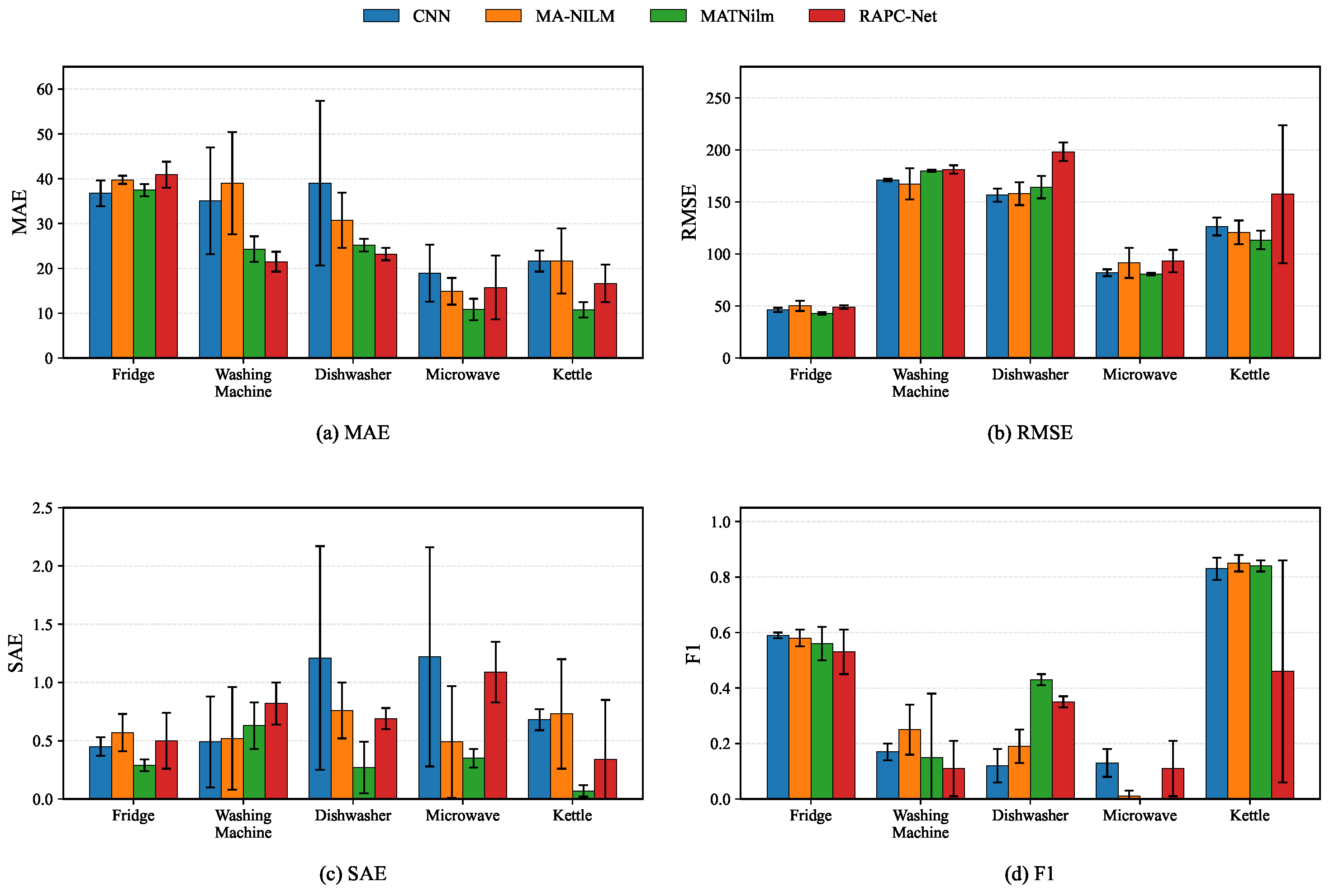
The appliance-level results in Figure 4 show that relative performance varies across appliance types. RAPC-Net performs favorably for the washing machine and dishwasher, which have relatively long operating durations and multi-stage power patterns. One possible explanation is that the shared temporal representation and residual-load modeling are suitable for distinguishing these structured load patterns from the remaining household consumption. However, this mechanism is not directly verified by the appliance-level comparison. RAPC-Net shows less evident advantages for the fridge, microwave, and kettle. The sparse and short-duration activations of the microwave and kettle may make their detection more sensitive to missed or underestimated events. The results may also reflect a trade-off between activation detection and physical consistency, but additional event-level analysis would be required to verify the underlying cause.

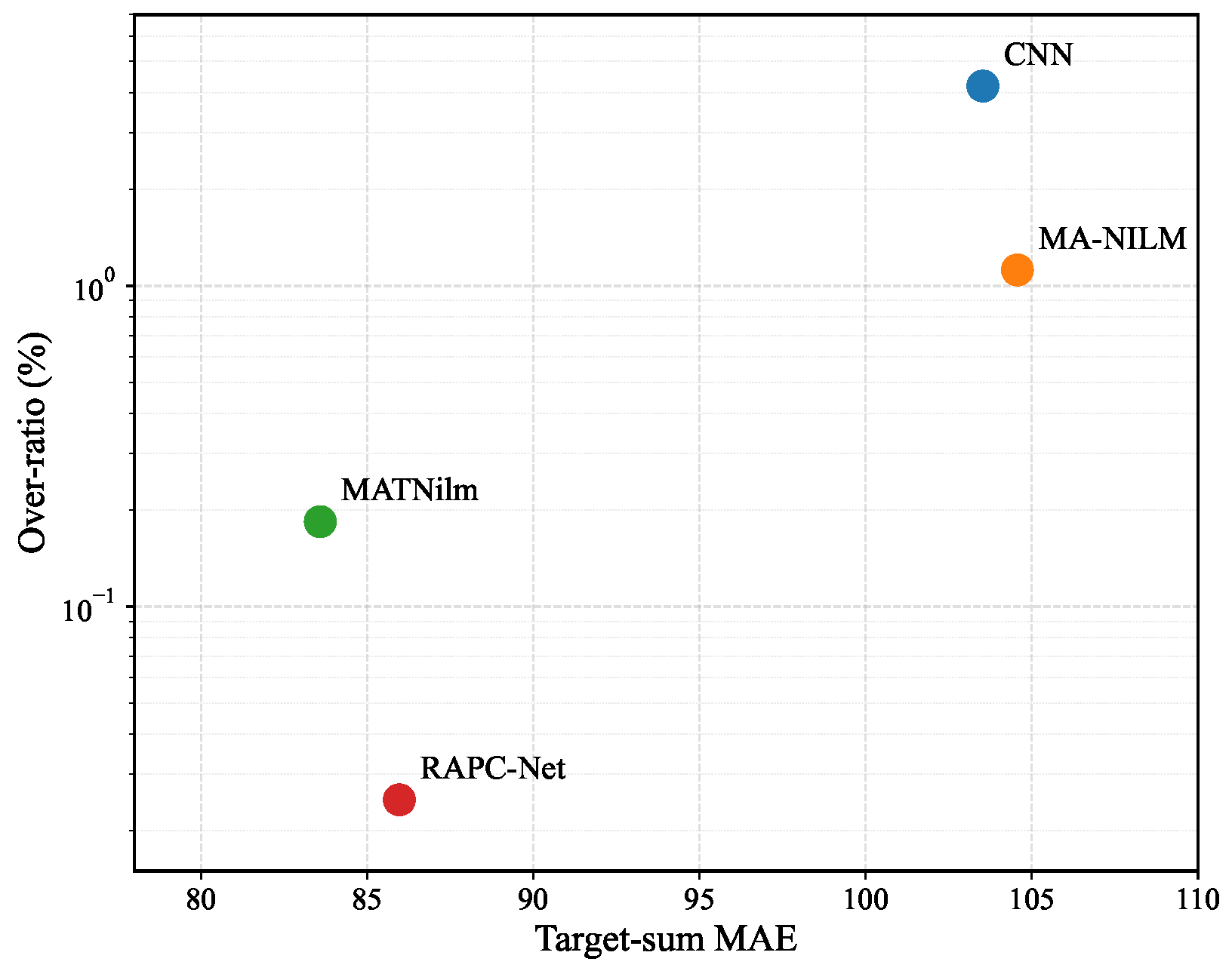
The main advantage of RAPC-Net is more evident in the joint estimation and physical consistency metrics. MATNilm achieves the lowest Target-sum MAE of $83.59\pm 3.71$ W, while RAPC-Net obtains a close value of $85.97\pm 15.45$ W. Meanwhile, RAPC-Net reduces the Over-ratio to $0.025\pm 0.020$% and the violation energy to $9.10\pm 5.47$ Wh, which are the lowest values among the compared methods. Figure 5 visualizes this relationship: RAPC-Net is close to MATNilm along the Target-sum MAE axis but has a substantially lower Over-ratio. Compared with CNN and MA-NILM, it also occupies a more favorable region on both dimensions. These observations suggest that the lower physical consistency errors cannot be explained solely by uniform suppression of the target-appliance predictions because the Target-sum MAE remains close to the best competing result.

This behavior is consistent with the intended roles of the proposed components. The residual branch represents household consumption that is not attributed to the selected target appliances. The aggregate reconstruction loss penalizes mismatches between the measured aggregate power and the power reconstructed from the target-appliance and residual predictions, while the one-sided overestimation loss directly penalizes cases in which the target-appliance sum exceeds the aggregate measurement. These properties provide a plausible explanation for the balance between Target-sum MAE and physical consistency observed under Case 1.

Case 2 provides an additional house-independent evaluation using a different combination of training, validation, and test households. As shown in

Table 8. Overall performance comparison under Case 2, reported as the mean and standard deviation across three runs with different random seeds.

Model	Avg. MAE (W)	Avg. RMSE (W)	Avg. SAE	Avg. F1	Target-Sum MAE (W)	Over-Ratio (%)	Violation Energy (Wh)
CNN	$40.87\pm 5.41$	$156.47\pm 6.52$	$0.628\pm 0.045$	$0.330\pm 0.052$	$129.25\pm 14.06$	$0.143\pm 0.060$	$93.10\pm 36.45$
MA-NILM	$37.01\pm 1.62$	$160.01\pm 14.58$	$0.413\pm 0.053$	$0.295\pm 0.067$	$133.69\pm 9.44$	$0.060\pm 0.051$	$20.66\pm 20.73$
MATNilm	$32.47\pm 1.62$	$156.39\pm 8.07$	$0.391\pm 0.092$	$0.314\pm 0.063$	$126.75\pm 8.96$	$0.028\pm 0.040$	$15.10\pm 23.20$
RAPC-Net	$39.32\pm 2.30$	$159.25\pm 10.54$	$0.403\pm 0.222$	$0.296\pm 0.029$	$127.29\pm 7.05$	$0.019\pm 0.011$	$10.14\pm 8.36$

, changing the household partition alters the relative appliance-level performance of all methods. MATNilm again achieves the lowest average MAE and shows strong overall appliance-level performance, whereas RAPC-Net does not consistently outperform the competing methods on the conventional appliance-wise metrics. The differences between Cases 1 and 2 suggest that appliance-level generalization is sensitive to household-specific characteristics, which may include appliance usage frequency, operating duration, power-state distribution, and unobserved household consumption.

At the joint target-appliance level, RAPC-Net achieves a Target-sum MAE of 127.29 ± 7.05 W, which is close to the lowest competing result of $126.75\pm 8.96$ W obtained by MATNilm and lower than the results of CNN and MA-NILM. RAPC-Net also achieves the lowest Over-ratio of $0.019\pm 0.011$% and the lowest violation energy of $10.14\pm 8.36$ Wh. Thus, its joint target-load error remains close to the best competing result under the second household partition, while its predicted target-appliance sum produces fewer and less severe aggregate-power violations.

The similar physical consistency trend across the two cases may be related to the household-level nature of the imposed constraints. Unlike appliance-specific temporal signatures, the requirement that the predicted target-appliance sum remain compatible with the measured aggregate power does not depend on a particular appliance operating pattern. Nevertheless, because only two household partitions are evaluated, these results should not be interpreted as establishing generalization across all households or datasets.

The Case 2 results also illustrate why physical feasibility should be evaluated together with conventional disaggregation metrics. A model may achieve lower appliance-wise errors while producing more frequent or larger aggregate-power violations. Conversely, a stronger emphasis on physical consistency may be accompanied by more conservative appliance estimates and lower activation-detection performance. RAPC-Net combines appliance-level supervision, residual-load modeling, aggregate reconstruction, and one-sided feasibility regularization to balance these objectives. Across the two evaluated cases, the resulting Target-sum MAE remains close to the best competing result, while the physical consistency errors are substantially reduced.

Overall, RAPC-Net does not uniformly achieve the best value for every appliance-level metric, and its relative appliance-wise performance varies between the two test households. Its consistent advantage lies in the physical compatibility of the jointly estimated target loads. In both house-independent comparisons, RAPC-Net maintains a Target-sum MAE close to the best competing method while achieving the lowest Over-ratio and violation energy. These results suggest that the principal benefit of RAPC-Net under the evaluated settings is improved physical feasibility of joint multi-appliance predictions rather than the uniform minimization of independent appliance-level errors. Such predictions may provide physically consistent inputs for subsequent household energy analysis, demand-response, and load-scheduling applications, although their downstream operational and economic effects are not evaluated in this study.

4.6. Computational Complexity

To assess the computational requirements of the evaluated methods,

Table 9. Computational complexity of the evaluated multi-appliance NILM methods.

Method	Parameters (M)	FLOPs (M)	Memory (MB)	Latency (ms/Window)
CNN	0.203	13.30	84.72	0.708
MA-NILM	0.996	45.68	213.47	3.462
MATNilm	0.230	114.54	1508.72	4.165
RAPC-Net	0.314	23.49	94.90	2.305

compares their parameter counts, floating-point operations (FLOPs), peak training memory, and per-window inference latency.

As shown in Table 9, CNN has the lowest parameter count, FLOPs, peak training memory, and inference latency, which is consistent with its relatively simple feedforward architecture. RAPC-Net contains 0.314 million parameters and requires 23.49 million FLOPs for a single input window. Compared with MA-NILM, RAPC-Net reduces the parameter count, FLOPs, peak training memory, and inference latency by approximately 68.5%, 48.6%, 55.5%, and 33.4%, respectively.

RAPC-Net contains more parameters than MATNilm but requires approximately 79.5% fewer FLOPs, 93.7% less peak training memory, and 44.7% lower inference latency. The relatively high FLOPs and memory consumption of MATNilm may be associated with its temporal and appliance-wise attention operations and the sizes of its intermediate feature representations. Overall, RAPC-Net has higher computational requirements than the basic CNN but lower FLOPs, memory consumption, and inference latency than MA-NILM and MATNilm under the evaluated setting. These results indicate that the residual-load branch and physical consistency formulation are incorporated with moderate additional computational requirements.

All models were evaluated on the same NVIDIA GeForce RTX 3060 GPU using TensorFlow 2.10. FLOPs were calculated for one forward pass with an input shape of $599\times 1$. Peak training memory was measured with a batch size of 128 during ten forward–backward optimization steps. Inference latency was measured with a batch size of one after 50 warm-up runs and averaged over 1500 forward passes. Parameter count and FLOPs describe model-level computational complexity, whereas memory consumption and latency depend on the hardware, software environment, and measurement protocol. The reported latency therefore represents a GPU-based comparison rather than performance on an embedded deployment platform.

4.7. Practical Implications and Limitations

A lower Over-ratio indicates fewer samples for which the predicted target-appliance sum exceeds the measured aggregate power. Violation energy additionally quantifies the cumulative magnitude of these violations. Under Case 1, RAPC-Net reduces the violation energy from $241.22$ Wh for MATNilm, which achieves the lowest value among the competing methods, to $9.10$ Wh over the same evaluation period. This result reflects an improvement in the joint target-load energy balance rather than only a reduction in the frequency of aggregate-power violations.

In downstream load-scheduling or demand-response applications, physically inconsistent appliance estimates may overstate the active or controllable demand and could consequently affect the feasibility of the resulting energy allocation. Reducing both Over-ratio and violation energy may therefore provide more physically consistent inputs for subsequent energy-management decisions. This interpretation is consistent with energy-management studies that connect electrical measurements and power-balance information with control actions and technical-economic indicators [29].

Nevertheless, RAPC-Net is evaluated as a NILM model rather than as a complete energy-management system. The experiments indicate improved physical consistency of joint target-appliance predictions under the evaluated settings, but they do not establish that RAPC-Net changes specific control decisions, improves scheduling feasibility, or reduces operating costs. Evaluating the proposed disaggregation framework within a downstream controller using scheduling and technical-economic indicators remains an important direction for future work.

The current RAPC-Net is primarily designed for offline load analysis. Its sequence-to-point formulation estimates the target time point from a centered window of 599 samples and therefore requires both past and future aggregate measurements. At the sampling interval of 8 s, the 299 future samples correspond to an algorithmic look-ahead delay of approximately 39.9 min. Although a trained model can process each complete window independently and may support delayed online monitoring, the current formulation is non-causal and is not intended for instantaneous control or real-time demand response. This look-ahead delay is distinct from the neural-network inference latency reported in Table 9. Future work will investigate causal or asymmetric input windows and lightweight streaming implementations for real-time deployment.

5. Conclusions

This paper proposed RAPC-Net for physically consistent multi-appliance NILM. The framework combines a shared temporal encoder, target-appliance and residual-load prediction branches, two watt-space physical consistency losses, and automatic appliance-aware weighting. The residual branch represents household consumption not attributed to the selected appliances, while the physical consistency losses penalize aggregate reconstruction errors and infeasible target-appliance sums. Appliance-aware weights are automatically derived from training-set activation statistics to address heterogeneous appliance activation patterns. Experiments on REFIT, including an expanded ablation study and two house-independent comparisons, suggest that residual-load modeling, physical consistency constraints, and appliance-aware weighting provide complementary contributions. Across both household partitions, RAPC-Net maintains competitive joint target-appliance estimation accuracy while consistently achieving the lowest Over-ratio and violation energy among the evaluated methods. These results indicate that its principal advantage lies in improving the physical feasibility of joint multi-appliance predictions rather than uniformly minimizing every appliance-level error metric.

The present study is limited to a fixed appliance set, two house-independent partitions from one dataset, and a single aggregated residual component. Moreover, the reported variability reflects three model initializations rather than independent household or temporal replicates. Future work will investigate more flexible residual modeling, adaptive weighting under changing appliance combinations, evaluation across additional datasets and households, rigorous statistical resampling, causal streaming implementations, and integration with downstream scheduling or demand-response systems.