The Optical Design and Calibration of a Finite-Conjugate VNIR Pushbroom Hyperspectral Camera for Close-Range Cultural Heritage Imaging

Abstract

Visible–near-infrared (VNIR) hyperspectral imaging provides a non-contact approach for cultural heritage examination. This study presents the design and calibration of a compact finite-conjugate VNIR pushbroom hyperspectral camera for close-range mural imaging. Operating over 400–1000 nm at a nominal working distance of 404 mm, the system provides a mean spectral sampling interval of 4.85 nm and an object-space sampling interval of approximately 82.4 μm/pixel. An integrated calibration workflow was established for wavelength assignment, spectral response characterization, geometric correction, radiometric calibration, and scan synchronization. The experimental results yielded a modulation transfer function (MTF) of 0.34 at the effective detector Nyquist frequency, a mean spectral response function full width at half maximum (FWHM) of 6.3 nm, a maximum absolute wavelength residual below 0.90 nm, residual smile and keystone errors below 0.3 pixels, a residual radiometric nonuniformity of 0.71%, and a mean signal-to-noise ratio (SNR) of 339. Measurements of Potala Palace mural samples demonstrate the acquisition of spatially detailed, radiometrically corrected hyperspectral data under close-range conditions.

1. Introduction

Cultural heritage conservation increasingly depends on non-invasive imaging to document material composition, monitor conservation treatments, and support reproducible interpretation. Conventional RGB photography and microscopic imaging provide detailed spatial records, but they cannot reliably distinguish materials with similar visible colors or reveal hidden, altered, or layered features. Visible–near-infrared (VNIR) hyperspectral imaging addresses this limitation by recording a spectrum at each spatial sample, allowing spectral differences to be analyzed together with surface morphology and spatial context [1,2,3].

For close-range diagnostics, an imaging instrument must satisfy more than a broad spectral range. It must provide object-space sampling sufficient to resolve brush strokes, cracks, retouching traces, and local material transitions. It must also preserve wavelength accuracy and spatial registration across the slit direction and the reconstructed scan direction. In pushbroom imaging, these requirements are strongly coupled because the hyperspectral cube is assembled from sequential line images rather than captured in a single exposure.

Existing cultural heritage studies have demonstrated the value of VNIR hyperspectral imaging for pigment mapping, manuscript examination, mural analysis, and degradation assessment [4,5,6,7,8,9,10,11,12,13,14]. Representative pushbroom systems can be configured for close-range imaging using focusable or interchangeable lenses. However, short-distance focusing alone does not establish system performance at a specified finite conjugate. Changing the object distance affects optical magnification, focus position, field coverage, object-space sampling, and spatial–spectral registration. Moreover, object-space sampling, end-to-end MTF, wavelength accuracy, and geometric residuals are not consistently reported under comparable close-range conditions. These quantities must therefore be re-established for the intended mural imaging geometry.

Finite-conjugate pushbroom imaging introduces several coupled challenges. Variations in object distance and surface relief produce spatially varying defocus and magnification, while sequential acquisition requires the scan-direction sampling interval to be matched to the slit-direction optical sampling interval. Scan speed fluctuations, trigger jitter, and dropped frames may cause geometric distortion and anisotropic sampling. In addition, wavelength assignment, smile, keystone, radiometric response, and relative reflectance conversion must remain stable under the selected working distance and illumination geometry. These requirements are not consistently evaluated together for close-range systems.

The contribution of this work lies in an experimentally validated finite-conjugate design, calibration, characterization, and evaluation workflow rather than short-distance focusing alone or a new Offner spectrograph principle. The main contributions are: (1) a design linking detector sampling pitch, working distance, focal length, instantaneous field of view (IFOV), depth of field, and object-space sampling; (2) the coordinated matching of the 82.4 μm slit-direction sampling interval to the 84.2 μm scan-direction interval; and (3) the experimental characterization of the MTF, wavelength accuracy, SRF FWHM, smile, keystone, radiometric nonuniformity, SNR, repeatability, and temperature-induced wavelength drift.

2. System Requirements and Derived Design Targets

2.1. Spectral Specifications

The effective operating range extends from λ_min = 400 nm to λ_max = 1000 nm. The spectral sampling interval is defined as the wavelength spacing between adjacent calibrated spectral channel centers. In contrast, spectral resolution describes the ability of the system to distinguish closely spaced spectral features and is experimentally characterized by the full width at half maximum (FWHM) of the spectral response function (SRF). For the developed system, the mean spectral sampling interval is 4.85 nm, whereas the measured mean spectral resolution is 6.3 nm. After the exclusion of saturated and low-response edge channels, 124 effective spectral channels were retained over the validated operating range.

$$\overline{\mathrm{\Delta }\lambda }={\displaystyle \frac{1 }{N_{eff}-1}}{\displaystyle \sum _{i=1}^{N_{eff}-1}({\lambda }_{c,i+1}-{\lambda }_{c,i})}$$

(1)

Although the silicon detector retains residual sensitivity beyond 1000 nm, the usable spectral range of the camera is determined by the end-to-end response of the detector, grating, optical coatings, order-sorting filter, and illumination source rather than by the intrinsic cutoff of the silicon detector alone. Beyond 1000 nm, the end-to-end system responsivity decreases substantially, resulting in reduced signal levels and less reliable spectral calibration. Wavelengths beyond 1000 nm were therefore excluded from the validated operating range. The reported range of 400–1000 nm represents the experimentally calibrated operating range of the complete system rather than the intrinsic sensitivity range of the silicon detector.

2.2. Spatial Sampling, Working Distance, and Depth of Field

The detector has a native pixel pitch of 6.5 μm. Three-pixel binning was applied in the spatial dimension, resulting in an effective detector sampling pitch p_eff of 19.5 μm. The effective focal length f = 95.6 mm was selected as an optical design input according to the finite-conjugate configuration and the required object-space sampling. The corresponding instantaneous field of view (IFOV) was calculated as

$$IFOV={\displaystyle \frac{p_{eff}}{f}}=0.204 \mathrm{m} \mathrm{rad}$$

(2)

At the nominal working distance L = 404 mm, the corresponding object-space sampling interval was calculated using the small-angle approximation:

$$\mathrm{\Delta }y=L\times IFOV\approx 82.4\mathsf{\mu }\mathrm{m}/\mathrm{pixel}$$

(3)

Therefore, the detector sampling pitch, focal length, and working distance were treated as design inputs, whereas the IFOV and object-space sampling interval were derived quantities.

The nominal working distance was selected by balancing object-space sampling, field coverage, illumination access, mechanical clearance, and sensitivity to mural surface relief. A shorter working distance provides finer object-space sampling but reduces the available mechanical clearance and generally increases sensitivity to defocus. Conversely, a longer working distance provides greater clearance but results in coarser object-space sampling. For example, working distances of 300, 404, and 500 mm correspond to nominal object-space sampling intervals of approximately 61.2, 82.4, and 102.0 μm/pixel, respectively. The selected distance of 404 mm therefore represents a practical compromise for the intended close-range scanning configuration rather than a universally optimal value.

The object-side depth of field was estimated using the geometrical optics approximation:

$$Depth of field\approx {\displaystyle \frac{2Nc(1+m)}{m^2}}$$

(4)

where N is the system F-number, c is the allowable image plane circle-of-confusion diameter, and m is the lateral magnification. The lateral magnification was estimated from the effective detector sampling pitch p_eff and the corresponding object-space sampling interval $\mathrm{\Delta }y$:

$$m={\displaystyle \frac{p_{eff}}{\mathrm{\Delta }y}}={\displaystyle \frac{19.5}{82.4}}\approx 0.237$$

(5)

In this analysis, one effective detector sampling interval was adopted as the allowable image plane blur diameter. Thus c = p_eff = 19.5 μm. Using N = 3, the estimated total object-side depth of field was approximately 2.6 mm, corresponding to approximately ±1.3 mm around the nominal object plane. This value is a first-order geometrical estimate based on a one-effective-pixel blur criterion. Surface height variations exceeding this range may produce local defocus and require refocusing.

2.3. Radiometric and Operational Requirements

For heritage diagnostics, radiometric repeatability and spectral fidelity are as important as spatial resolution. For each dataset, the exposure time, detector gain, detector temperature, camera line rate, scan speed, working distance, illumination geometry, firmware version, and reconstruction software version were recorded. The adopted performance targets were a mean signal-to-noise ratio above 300, wavelength calibration accuracy better than 1 nm, residual smile and keystone errors below 0.3 pixels, and residual radiometric nonuniformity below 1%. The main system specifications and design constraints are summarized in

Table 1. System specifications and design constraints.

Parameter	Value
Validated spectral range	400–1000 nm
Spectral sampling interval	4.85 nm
Effective channel count	124
Working distance	404 mm
IFOV	0.204 mrad
Effective sampling pitch	19.5 μm
Native detector pixel pitch	6.5 μm
Object-space sampling interval	82.4 μm/pixel
Effective focal length	95.6 mm
F-number	3
Mean SNR	≥300
Wavelength accuracy target	≤1 nm
Smile/keystone residual target	≤0.3 pixels
Residual radiometric nonuniformity target	≤1%

.

3. Optical Architecture and System Overview

The camera adopts a pushbroom dispersive architecture. A slit defines one spatial dimension, while the spectrograph maps wavelength onto the orthogonal detector dimension. The second spatial dimension is generated by controlled relative motion between the camera and the object.

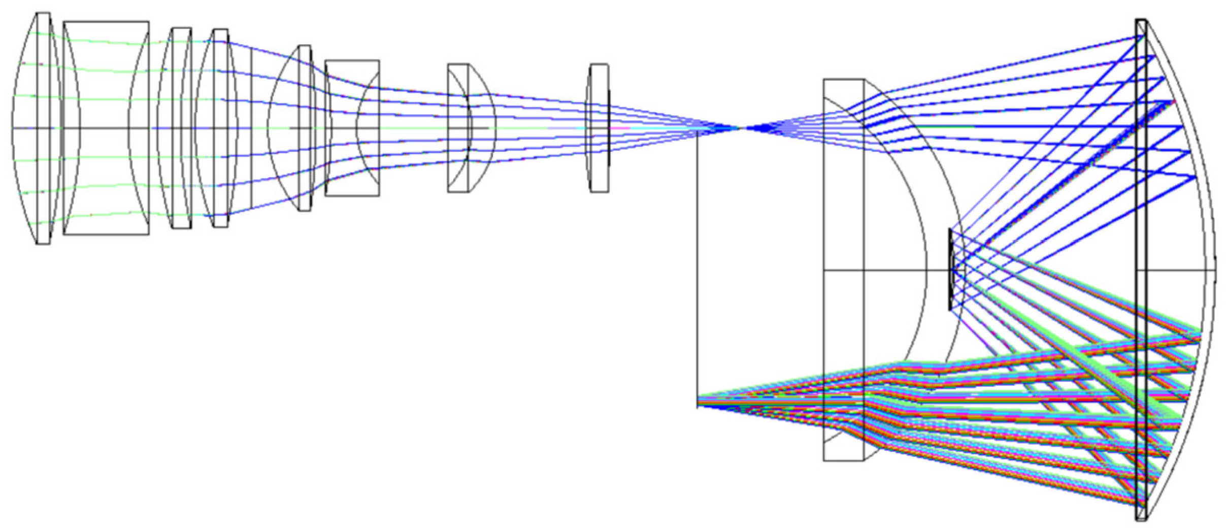
The optical system consists of finite-conjugate fore-optics, an entrance slit, an Offner imaging spectrograph, and a silicon complementary metal–oxide–semiconductor (CMOS) detector. The detector has a native format of 2048 × 2048 pixels and a pixel pitch of 6.5 μm. In the spatial direction, 2040 valid detector pixels were retained, and three-pixel binning was applied, resulting in 680 effective spatial samples with an effective sampling pitch of 19.5 μm. The remaining eight edge pixels were excluded during preprocessing. Two-pixel binning in the spectral direction provides an effective sampling pitch of 13 μm. After invalid edge channels were excluded, 124 effective spectral channels were retained over 400–1000 nm, corresponding to a mean spectral sampling interval of 4.85 nm. The optical layout of the developed finite-conjugate VNIR pushbroom hyperspectral camera is shown in Figure 1.

The Offner spectrograph has a nominal slit-to-detector magnification close to unity. A 13 μm entrance slit was selected so that its image approximately matched one effective detector sampling pitch in the spectral direction while maintaining sufficient optical throughput. The slit length was 15.6 mm. The spectrograph employs a convex reflective grating with a groove density of 90 lines/mm and a blaze wavelength of 550 nm and operates in the first diffraction order. The Offner configuration was selected for its compact layout and its ability to control spatial and spectral aberrations over 400–1000 nm. The main detector, slit, and grating parameters are summarized in

Table 2. Instrument parameter table.

Parameter	Value
Spectrograph configuration	Offner
Detector manufacturer	Fairchild Imaging
Detector model	CIS2521
Detector technology	CMOS
Detector material	Silicon
Native detector format	2048 × 2048
Native pixel pitch	6.5 μm
Effective sampling pitch	19.5 μm
Detector active area	13.312 mm × 13.312 mm
Entrance slit width	13 μm
Entrance slit length	15.6 mm
Grating type	Convex reflective grating
Groove density	90 lines/mm
Blaze wavelength	550 nm
Diffraction order	First order
System F-number	3
Working distance	404 mm

.

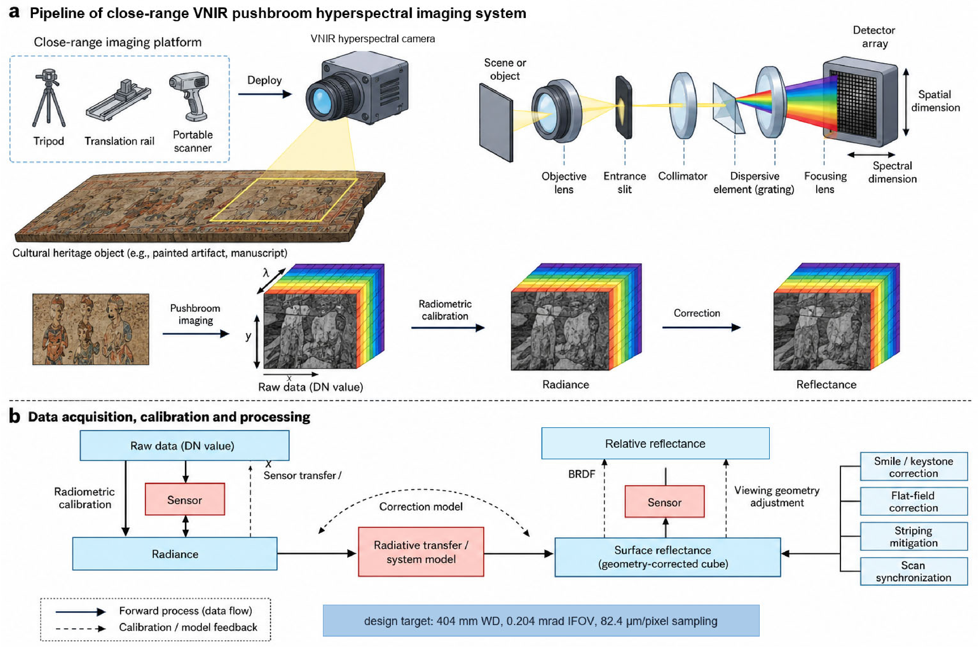
The coordinate convention was defined to avoid ambiguity during calibration and data cube reconstruction. The slit direction defines the spatial y-axis, the scan direction defines the reconstructed spatial x-axis, and the detector dispersion coordinate p is mapped to wavelength λ through wavelength calibration. The reconstructed hyperspectral data cube is represented as I(x,y,λ). The overall system configuration, coordinate definitions, and hyperspectral data acquisition and processing workflow are illustrated in Figure 2.

4. Optical Design and Performance Analysis

4.1. Design Inputs

The numerical design inputs are summarized in Table 1 and Table 2. The finite-conjugate optical configuration was optimized over 400–1000 nm at the nominal object distance of 404 mm. The principal optimization targets included slit-direction MTF, spectral line width, field-dependent wavelength shift, relative illumination, and magnification stability. The design also considered object distance variation because mural relief and imperfect target positioning may produce spatially varying defocus.

4.2. Aberration Control Strategy

The optical design prioritizes spatial performance along the slit, a stable spectral line shape in the dispersion direction, and limited spectral–spatial coupling. Astigmatism, field curvature, coma, detector tilt, and relative illumination are controlled across representative field points and wavelengths. In the spectral direction, optimization focuses on maintaining stable SRF width and reducing field-dependent wavelength shifts.

4.3. Simulated Spatial Performance

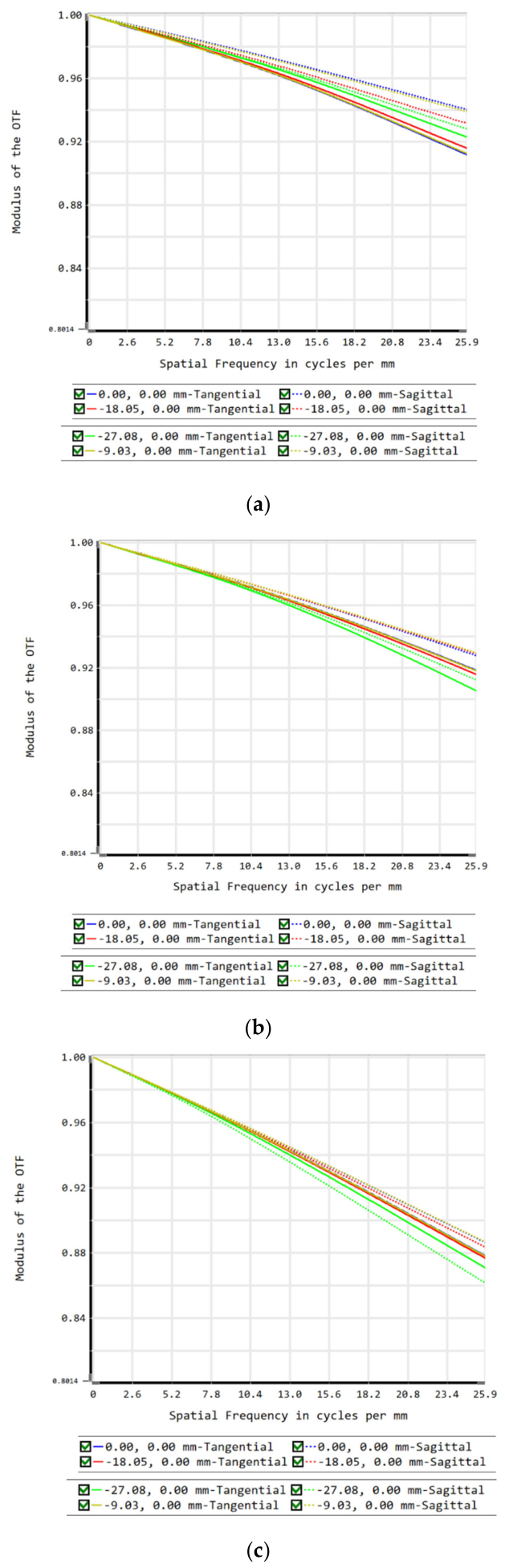
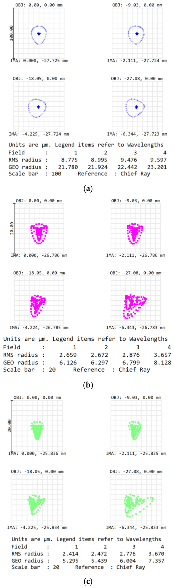
The slit-direction MTF was evaluated at the center, intermediate, and edge field positions at wavelengths of 0.4, 0.7, and 1.0 μm. Both sagittal and tangential MTF curves are presented for each field position. As shown in Figure 3, the nominal optical MTF remains above 0.87 at the effective detector Nyquist frequency of 25.64 lp/mm. The corresponding spot diagrams at four representative field positions and wavelengths of 0.4, 0.7, and 1.0 μm are shown in Figure 4.

5. Tolerance Analysis and Alignment Strategy

5.1. Tolerance Allocation

Tolerance analysis was performed to relate mechanical and optical perturbations to the predicted optical MTF. The analyzed variables included slit decenter and tilt, grating tip/tilt, optical element decenter, detector defocus and tilt, and stop position error. The tolerance limits are summarized in

Table 3. Key tolerance items and allocated limits.

Parameter	Value
Radius/mm	±0.01
Thickness/mm	±0.02
Decenter/mm	±0.01
Tilt/°	±0.02

. A total of 500 Monte Carlo trials were performed using the allocated tolerances. As shown in

Table 4. Results of system tolerance analysis.

Monte Carlo Probability/%	MTF@25.64 lp/mm
90	0.64211
70	0.68356
50	0.71244
30	0.75328

, 90% of the simulated optical systems had an optical MTF greater than 0.642 at the effective detector Nyquist frequency of 25.64 lp/mm.

The simulated and measured MTF values represent different levels of the imaging chain and should not be compared directly. The nominal value above 0.87 and the 90% probability value of 0.642 describe the optical subsystem in the design and tolerance models. Assuming a rectangular detector sampling aperture with a unity fill factor, the detector aperture MTF at the effective Nyquist frequency is 2/π = 0.637. The corresponding tolerance-degraded optical detector estimate is therefore approximately 0.642 × 0.637 = 0.409. The experimentally measured end-to-end MTF is 0.34, approximately 17% below this estimate. The remaining difference may arise collectively from finite slit averaging, residual defocus, target contrast, scan motion, sampling phase effects, and measurement uncertainty. Because these contributions were not independently isolated, the reduction is not attributed solely to fabrication and alignment errors. The MTF values at different levels of the imaging chain are summarized in

Table 5. Comparison of optical, detector aperture, and measured end-to-end MTF values.

MTF Level	Value at Nyquist
Nominal optical design	0.870
Tolerance-degraded optical MTF	0.642
Detector aperture MTF	0.637
Optical detector estimate	0.409
Measured end-to-end MTF	0.340

.

$$MT{F}_{pixel }=sinc({\displaystyle \frac{\pi }{2}}) \approx 0.637$$

(6)

$$MT{F}_{optical-detector} =0.642\times 0.637\approx 0.409$$

(7)

5.2. System Alignment Procedure

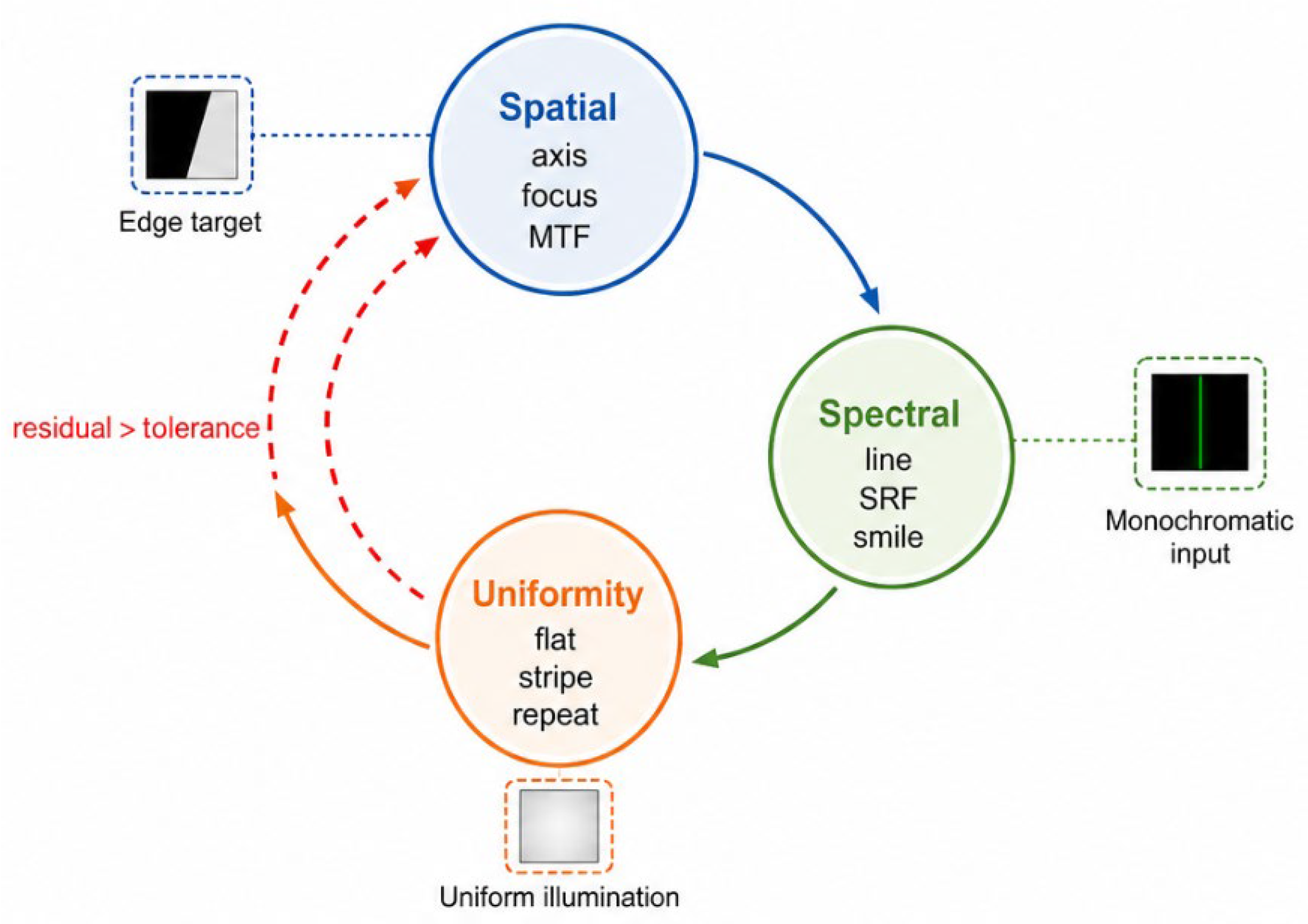
The alignment procedure proceeded from spatial alignment to spectral alignment and finally to radiometric uniformity adjustment. First, the optical axis and focus were established using collimated targets, edge targets, and slit-direction MTF measurements. Second, monochromatic illumination was used to adjust the grating and detector according to spectral line position, line shape, and wavelength residual. Finally, uniform illumination was used to complete flat-field correction and repeatability evaluation. The sequential workflow for spatial, spectral, and radiometric alignment is illustrated in Figure 5. The sensitivity ranking of representative tolerance items with respect to the main system performance metrics is summarized in

Table 6. Sensitivity ranking of representative tolerance items.

Tolerance Item	MTF	Wavelength RMS	SRF FWHM	Smile	Keystone	Uniformity
Slit decenter	High	Medium	Low	Medium	High	Low
Slit tilt	Medium	Medium	Medium	High	High	Low
Grating tip/tilt	Low	High	High	High	Medium	Low
Detector defocus	High	Medium	High	Medium	Medium	Low
Detector tilt	High	High	High	High	High	Low
Illumination nonuniformity	Low	Low	Low	Low	Low	High
Scan jitter	Medium	Low	Low	Low	Medium	Medium

.

6. Calibration Methodology

6.1. Metadata Fixation and Raw Preprocessing

All calibration datasets were acquired using fixed and recorded exposure time, detector gain, detector temperature, line rate, scan speed, working distance, and illumination geometry. Dark frames were collected under the same camera settings with the optical input blocked. Bad pixels, saturated pixels, and unstable spectral channels were rejected using the same predetermined thresholds for all datasets.

6.2. Wavelength Calibration

Wavelength calibration was performed using a tungsten–halogen lamp coupled to a monochromator. The monochromator had a nominal wavelength accuracy of 0.2 nm and an output bandwidth of 0.5 nm. It was scanned from 400 to 1000 nm with a wavelength step of 0.5 nm. At each wavelength, 20 frames were acquired and averaged after dark subtraction. The center position of each monochromatic response was estimated by Gaussian fitting. A third-order polynomial was then used to establish the detector pixel-to-wavelength mapping λ(p). Calibration performance was evaluated using the root-mean-square (RMS) residual and maximum absolute residual.

6.3. Spectral Response Function Characterization

The spectral response function (SRF) was measured by scanning the monochromator across each selected channel using a wavelength step of 0.5 nm. At each wavelength, 20 frames were averaged after dark subtraction. The measured response was normalized and fitted using a Gaussian function. The center wavelength and full width at half maximum (FWHM) were obtained from the fitted curve. The procedure was repeated five times, and the mean and standard deviation of the SRF FWHM were calculated over the retained spectral range.

6.4. Smile and Keystone Mapping and Correction

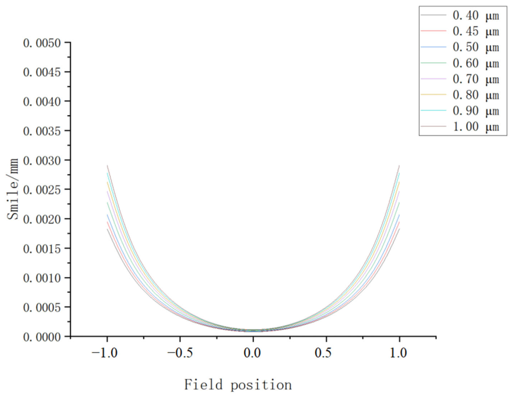
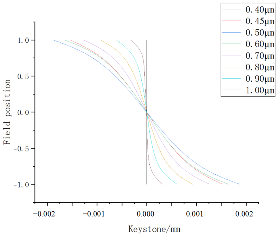
Smile was measured as the displacement of the fitted monochromatic line center along the detector dispersion direction as a function of position along the entrance slit. Measurements were performed at 450, 550, 700, 850, and 950 nm using five equally spaced slit positions. Keystone was measured as the wavelength-dependent displacement of the same spatial target feature along the slit direction relative to the reference channel at 700 nm. A second-order polynomial correction and cubic interpolation were applied to resample the data onto a common spatial–spectral grid. The smile and keystone distributions at representative wavelengths are shown in Figure 6 and Figure 7.

6.5. Radiometric Calibration and Relative Reflectance Conversion

Radiometric calibration was performed to establish the relationship between the detector digital number (DN) and the input spectral radiance. A calibrated integrating sphere with known spectral radiance was used as the reference source. The integration time, detector gain, working distance, and optical configuration were kept unchanged during calibration, and dark frames were acquired with the optical input blocked.

For each spectral channel, the camera response was measured at five radiance levels within the linear response range of the detector. At each radiance level, 100 frames were averaged to reduce temporal noise. The relationship between the dark-corrected camera response and the reference spectral radiance was fitted using the following:

$$L_j (\lambda )=a(\lambda )[D{N}_j (\lambda )-D{N}_{dark} (\lambda )]+b(\lambda )$$

(8)

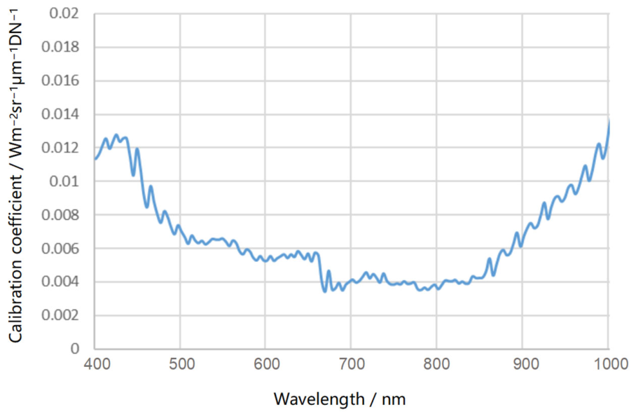
where L_j(λ) is the reference spectral radiance at the j-th radiance level, DN_j(λ) is the corresponding camera output, DN_dark(λ) is the dark frame response, a(λ) is the wavelength-dependent radiometric calibration coefficient, and b(λ) is the residual offset. Figure 8 shows the wavelength-dependent radiometric calibration coefficient a(λ). The coefficient is relatively low in the central spectral region and increases toward the short- and long-wavelength limits. Because the radiometric calibration coefficient is inversely related to the overall system responsivity, the larger coefficient values near the spectral limits indicate a lower combined response of the optical system, diffraction grating, and silicon detector in these regions.

Pixel-to-pixel response nonuniformity was additionally corrected using a uniform integrating sphere image. For each wavelength channel, the dark-corrected response of each valid spatial pixel was normalized to the mean dark-corrected response of all valid spatial pixels. The relative nonuniformity correction coefficient was calculated as follows:

$$K_i={\displaystyle \frac{\overline{DN}(\lambda )-D{N}_{dark}(\lambda )}{D{N}_i(\lambda )-D{N}_{dark,i}(\lambda )}}$$

(9)

where DN_i(λ) and DN_dark,i(λ) are the illuminated and dark responses, and the numerator represents the mean dark-corrected response of all valid spatial pixels. After correction, the mean residual spatial nonuniformity over 400–1000 nm was 0.71%.

The normalized end-to-end spectral responsivity was derived from the inverse spectral radiance calibration coefficient:

$$S_{rel} (\lambda )={\displaystyle \frac{1/a(\lambda )}{\max [1/a(\lambda )]}}$$

(10)

where a(λ) is the spectral radiance calibration coefficient, and S_rel(λ) is the normalized relative system spectral responsivity. For cultural heritage measurements, a diffuse white reference panel with a nominal reflectance of 0.99 was used to convert the camera responses into relative reflectance. White reference, sample, and dark frames were acquired using the same illumination geometry, working distance, integration time, detector gain, and optical configuration. The relative reflectance of the sample was calculated as follows:

$$R_{sample} (\lambda )={\displaystyle \frac{D{N}_{sample} (\lambda )-D{N}_{dark} (\lambda ) }{D{N}_{white} (\lambda )-D{N}_{dark} (\lambda )}}{R}_{white} (\lambda )$$

(11)

where DN_sample(λ), DN_white(λ), and DN_dark(λ) are the sample, white reference, and dark responses, respectively, and R_white(λ) = 0.99 was adopted as the nominal reflectance of the diffuse white panel. Because a certified wavelength-dependent reflectance curve of the panel was unavailable, the resulting spectra are reported as relative rather than absolute reflectance. Saturated channels and channels with an SNR below 100 were excluded. The resulting spectra therefore represent relative reflectance under the specified measurement geometry rather than raw detector DN values.

6.6. Scan Synchronization and Reconstruction

Motion synchronization was implemented using hardware triggering and encoder-based position recording. The platform scan speed v and camera line rate f_line determine the scan-direction sampling interval according to the following:

$$\mathrm{\Delta }{x}_{scan}= {\displaystyle \frac{v}{f_{line}}}$$

(12)

At the nominal working distance of 404 mm, the slit-direction object-space sampling interval was approximately 82.4 μm. With a platform scan speed of 23.15 mm/s and a camera line rate of 275 Hz, the nominal scan-direction sampling interval was

$$\mathrm{\Delta }{x}_{scan}={\displaystyle \frac{23.15}{275}}=84.2\mathrm{\mu }\mathrm{m}$$

(13)

The difference between the slit- and scan-direction sampling intervals was approximately 2.2%, providing a nearly uniform spatial sampling grid in the reconstructed hyperspectral cube. During acquisition, trigger timestamps, encoder positions, velocity fluctuations, and dropped line flags were recorded. The encoder-derived position–time trajectory was subsequently used to correct scan speed variations and resample the acquired line images onto a uniform spatial grid. The calibrated line images were then assembled into a hyperspectral data cube represented as I(x,y,λ).

7. Experimental Characterization and Demonstration

7.1. Experimental Setup

The experimental characterization setup included a spatial bar target, a tungsten–halogen lamp coupled to a monochromator, a calibrated integrating sphere, a diffuse white reference standard, and heritage-relevant samples. Spatial performance was evaluated using the bar target, spectral performance was evaluated using the monochromator, and radiometric performance was evaluated using the calibrated integrating sphere. Close-range imaging was demonstrated using Potala Palace mural samples.

Before each measurement series, the camera was operated for 30 min to reach thermal stability. The MTF, SRF FWHM, smile, keystone, radiometric nonuniformity, and SNR measurements were independently repeated five times. Each repetition included the reacquisition of the raw data and repetition of the complete processing procedure. The results are reported as the mean ± standard deviation. The 95% confidence interval of the mean was calculated using Student’s t-distribution:

$$C{I}_{95\%} =\overline{x}\pm t_{0.975,n-1} {\displaystyle \frac{s}{\sqrt{n}}}$$

(14)

where $\overline{x}$ is the sample mean, s is the sample standard deviation, and n is the number of repeated measurements.

7.2. Spatial Performance

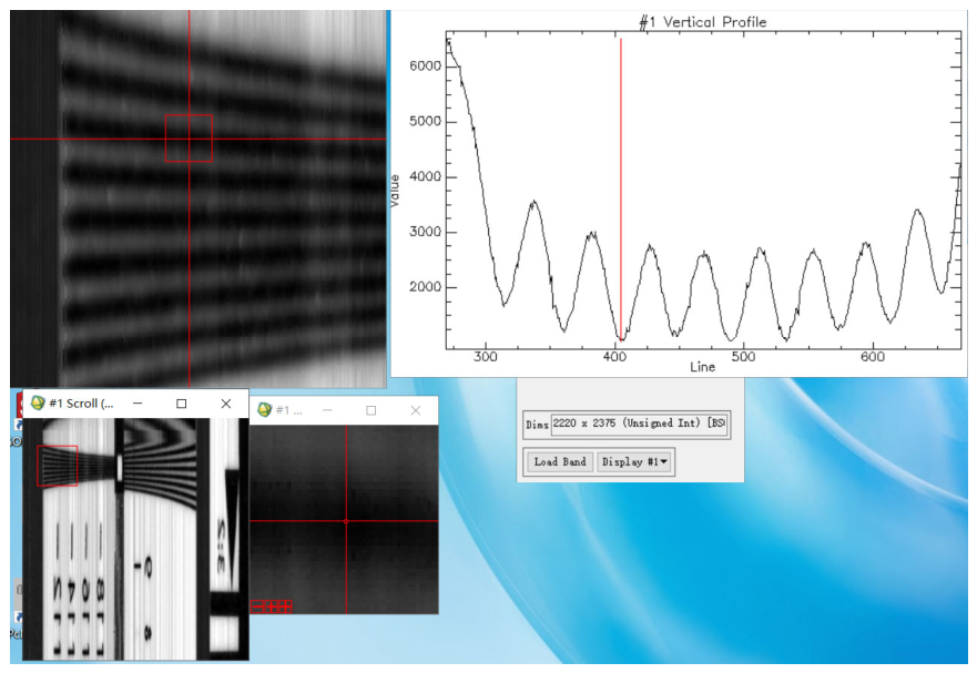
The end-to-end spatial MTF was evaluated using a standard bar target method under the nominal close-range imaging configuration. A 100× bar target was imaged by the hyperspectral camera, and the bar pattern corresponding to the effective detector Nyquist frequency was selected. The responses of the white and black bar regions were extracted as DN_w and DN_b, respectively. To reduce sampling phase bias, the target position providing the maximum stable black–white contrast was used. The equivalent sinusoidal MTF was calculated as

$$MTF={\displaystyle \frac{D{N}_w-D{N}_b}{D{N}_w+D{N}_b}}\times {\displaystyle \frac{\pi }{4}}$$

(15)

where (DN_w − DN_b)/(DN_w + DN_b) represents the measured bar pattern modulation, and π/4 is the conversion factor from square-wave modulation to the equivalent sinusoidal MTF. The obtained value was used to evaluate the spatial imaging performance of the spectrometer at the Nyquist frequency. The acquired bar target image and extracted intensity profile are shown in Figure 9, while the measured DN values and calculated end to end MTF are summarized in

Table 7. The end-to-end MTF measured using the bar target method.

Parameter	Channel	Value	Average	MTF
VNIR	DNw	2566	2694	0.34
		2799
		2717
	DNb	1153	1061
		1013
		1017

.

7.3. Spectral Performance

Spectral performance was evaluated by wavelength calibration and spectral response function (SRF) measurement. The spectral sampling interval was defined as the spacing between adjacent channel center wavelengths, while the spectral resolution was characterized by the full width at half maximum (FWHM) of each SRF.

Spectral measurements were performed under the nominal finite-conjugate configuration at a working distance of 404 mm. A tungsten–halogen lamp was coupled to the monochromator, and the monochromator output illuminated a diffuse reflectance panel positioned at the nominal object plane. The integration time and detector gain were kept fixed during each scan, and the source intensity was adjusted to maintain the detector response within its linear range.

For each spectral channel, the measured response curve was fitted with a Gaussian function to determine the center wavelength λ_c,i and FWHM. The spectral sampling interval and spectral resolution were calculated as

$$\mathrm{\Delta }{\lambda }_{\mathrm{sampling},i}={\lambda }_{c,i+1}-{\lambda }_{c,i}$$

(16)

$$\mathrm{\Delta }{\lambda }_{\mathrm{resolution},i}=FWH{M}_i$$

(17)

The mean spectral sampling interval was 4.85 nm, whereas the mean SRF FWHM over the validated VNIR range was 6.3 nm. The ratio of the mean SRF FWHM to the sampling interval was approximately 1.3, indicating that the channel spacing was smaller than the measured spectral resolution. Across five repeated measurements, the wavelength-averaged SRF FWHM was 6.3 ± 0.20 nm. The corresponding 95% confidence interval was 6.05–6.55 nm.

The wavelength calibration residual was defined as the difference between the fitted center wavelength and the reference wavelength:

$${\epsilon }_i={\lambda }_{c,i}-{\lambda }_{\mathrm{ref},i}$$

(18)

The calibration accuracy was evaluated using the root-mean-square error and the maximum absolute residual:

$$RMS{E}_{\lambda }=\sqrt{{\displaystyle \frac{1}{N}}{\displaystyle \sum _{i=1}^N{\epsilon }_i^2}},\hspace{1em}{\epsilon }_{\max }=\max (|{\epsilon }_i|)$$

(19)

The wavelength calibration uncertainty was estimated from the main uncertainty contributors, including monochromator wavelength setting, monochromator spectral bandwidth, measurement repeatability, Gaussian peak fitting, and wavelength mapping residual. The wavelength calibration RMSE was 0.18 nm, and the maximum absolute residual was below 0.90 nm over the validated spectral range. The uncertainty budget is summarized in

Table 8. Uncertainty budget for wavelength calibration.

Source of Uncertainty	Symbol	Standard Uncertainty/nm
Monochromator wavelength setting	$u_{\mathrm{mono}}$	0.18
Monochromator spectral bandwidth	$u_{\mathrm{band}}$	0.12
Measurement repeatability	$u_{\mathrm{rep}}$	0.12
Gaussian peak fitting	$u_{\mathrm{fit}}$	0.18
Wavelength mapping residual	$u_{\mathrm{map}}$	0.18
Combined standard uncertainty	$u_c$	0.36
Expanded uncertainty (k = 2)	U	0.72

. Assuming that these terms are independent, the combined standard uncertainty was calculated as follows:

$$u_c(\lambda )=\sqrt{u_{\mathrm{mono}}^2+u_{\mathrm{band}}^2+u_{\mathrm{rep}}^2+u_{\mathrm{fit}}^2+u_{\mathrm{map}}^2}$$

(20)

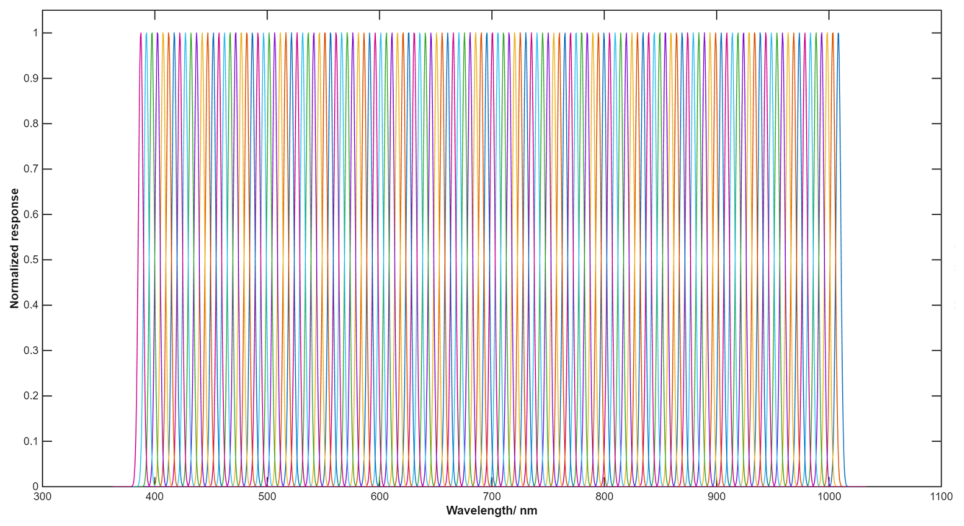
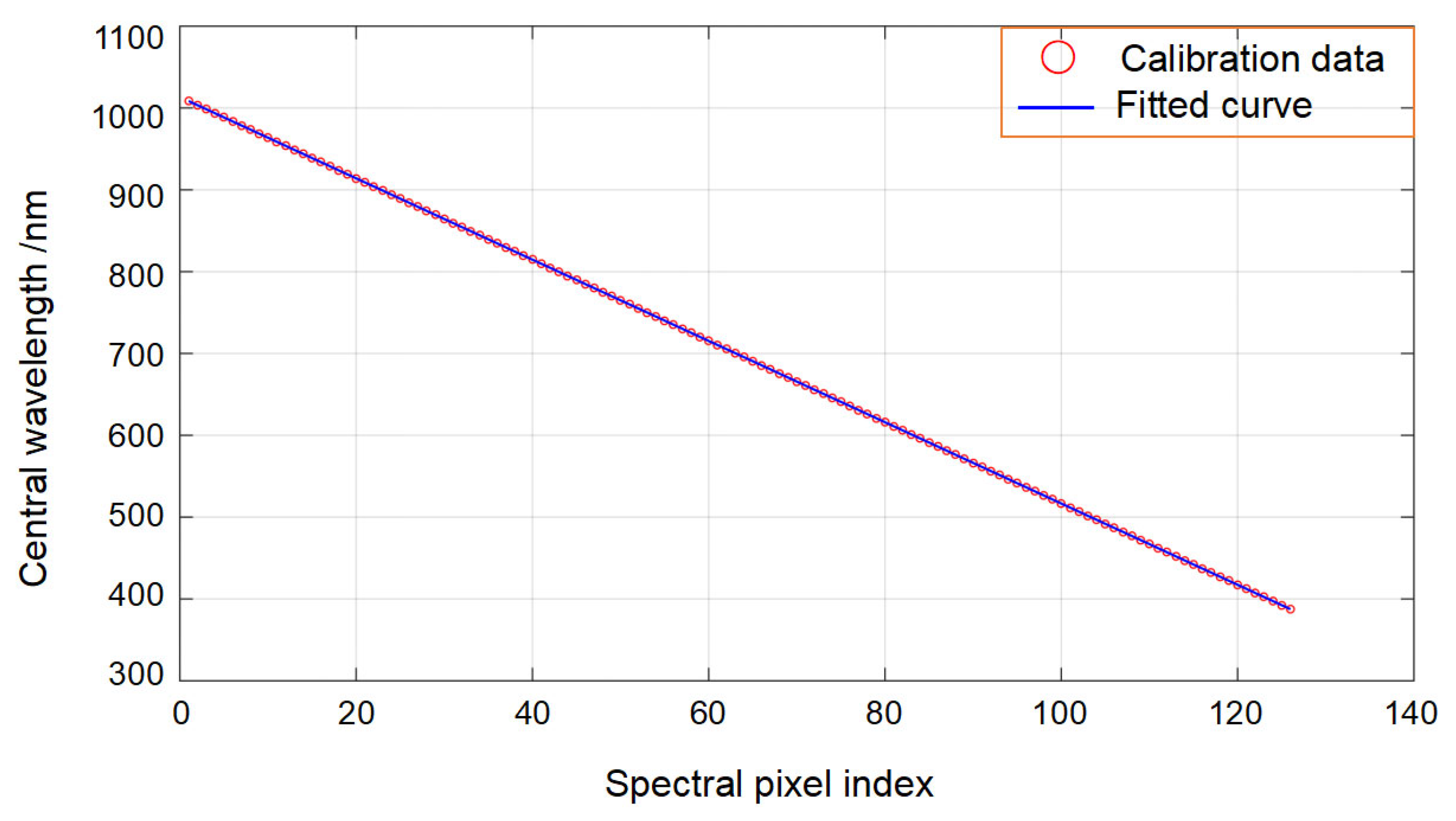
The combined standard uncertainty was 0.36 nm. Using a coverage factor of k = 2, the expanded uncertainty was 0.72 nm, corresponding to an approximate 95% level of confidence. The expanded uncertainty was below the specified wavelength calibration requirement of 1 nm. The measured normalized spectral response functions across the VNIR range are shown in Figure 10, and the fitted pixel to wavelength calibration relationship is presented in Figure 11.

The standard uncertainty components were obtained from the monochromator calibration certificate, repeated measurements, Gaussian fitting results, and wavelength mapping residuals.

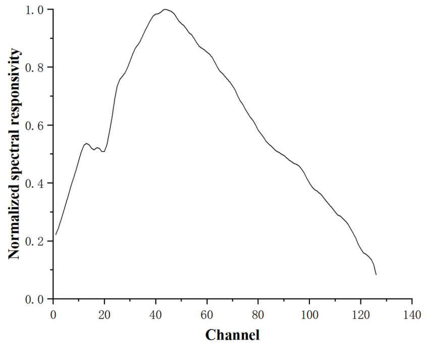
The normalized end-to-end system spectral responsivity was calculated from the inverse of the spectral radiance calibration coefficient and normalized to its maximum value. As shown in Figure 12, the response is the highest in the central spectral region and decreases toward both spectral limits. This trend results from the combined wavelength-dependent efficiencies of the optical system, diffraction grating, and silicon detector.

7.4. Signal-to-Noise Ratio Measurement

The signal-to-noise ratio (SNR) was measured under uniform illumination to evaluate the radiometric sensitivity of the hyperspectral camera. A blackbody source coupled to an integrating sphere was used to provide uniform illumination. The integration time and detector gain were adjusted to maintain the detector response within its linear range and were then kept unchanged throughout the measurement. After the system had stabilized, 100 illuminated hyperspectral frames were continuously acquired. Dark frames were subsequently recorded using the same camera settings with the optical input blocked.

For each wavelength channel, the mean digital number (DN) within a fixed uniform spatial region of interest was extracted from each frame. The mean dark response was calculated from the acquired dark frames and subtracted from each illuminated frame response. The wavelength-dependent SNR was then calculated from the dark-corrected mean signal and the temporal standard deviation of the illuminated frame responses as follows:

$$\mathrm{SNR}(\lambda )={\displaystyle \frac{{\overline{\mathrm{DN}}}_{\mathrm{ill}}(\lambda )-{\overline{\mathrm{DN}}}_{\mathrm{dark}}(\lambda )}{\sqrt{\frac{1}{N-1}{\displaystyle \sum _{i=1}^N{\left[{\mathrm{DN}}_{\mathrm{ill},i}(\lambda )-{\overline{\mathrm{DN}}}_{\mathrm{ill}}(\lambda )\right]}^2}}}},\hspace{1em}\hspace{1em} N=100$$

(21)

where DN_ill,i(λ) is the response of the i-th illuminated frame at wavelength λ, $\overline{D{N}_{ill}}(\lambda )$ is the mean response of the 100 illuminated frames and $\overline{D{N}_{dark}}(\lambda )$ is the mean dark response acquired using the same camera settings. The resulting SNR curve was reported over the retained 400–1000 nm spectral range.

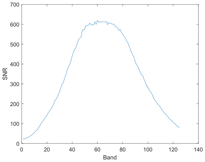
The wavelength-averaged SNR over the retained 400–1000 nm channels was 339, with a peak value of 613 in the central spectral region. As shown in Figure 13, the SNR increases from the short-wavelength end, reaches its maximum in the central spectral region, and then decreases toward the long-wavelength end. This wavelength-dependent trend is mainly attributed to the combined effects of the illumination spectrum, optical throughput, grating diffraction efficiency, and detector quantum efficiency. The lower SNR values near the two spectral limits indicate reduced end-to-end system responsivity and a relatively larger noise contribution, whereas the higher SNR in the central channels indicates adequate radiometric sensitivity under the specified close-range acquisition conditions. Repeatability statistics from five independent measurements are summarized in

Table 9. Repeatability statistics for the measured system performance metrics.

Metric	Repetitions	Mean	Standard Deviation	95% Confidence Interval
MTF at Nyquist	5	0.34	0.02	0.32–0.36
SRF FWHM	5	6.3 nm	0.20 nm	6.05–6.55 nm
Mean SNR	5	339	12	324–354
Residual nonuniformity	5	0.71%	0.04%	0.66–0.76%
Residual smile RMS	5	0.18 pixels	0.02 pixels	0.16–0.20 pixels
Residual keystone RMS	5	0.21 pixels	0.02 pixels	0.19–0.23 pixels

.

7.5. Temperature Stability

Temperature stability was evaluated over a controlled cooling–heating cycle, in which the ambient temperature was decreased from 20 °C to 10 °C and subsequently increased to 30 °C. The camera remained powered on throughout the experiment, while the integration time, detector gain, optical configuration, illumination, and monochromator settings were kept unchanged. The center wavelength of a 550 nm monochromatic input was measured at 5 min intervals and determined by Gaussian fitting. The initial measurement at 20 °C was used as the reference, and the wavelength drift was calculated as follows:

$$\mathrm{\Delta }\lambda (t)={\lambda }_c (t)-{\lambda }_c (t_0)$$

(22)

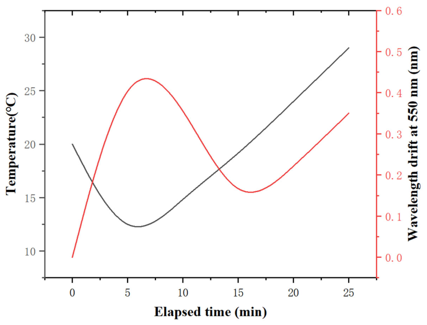
where λ_c(t) is the fitted center wavelength at time t, and t₀ denotes the initial measurement at 20 °C. During the 20–10–30 °C set-point cycle, the maximum absolute wavelength drift at 550 nm was 0.42 nm. This drift was below the specified wavelength accuracy requirement of 1 nm but was comparable in magnitude to the combined standard uncertainty of 0.36 nm. Therefore, temperature monitoring and stabilization are recommended for wavelength-sensitive measurements. The measured temperature variation and corresponding wavelength drift during the cooling heating cycle are shown in Figure 14.

7.6. Cultural Heritage Demonstration

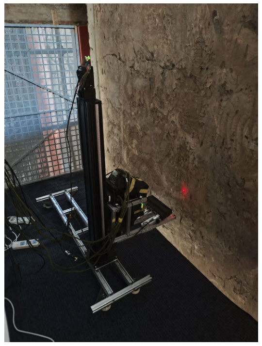
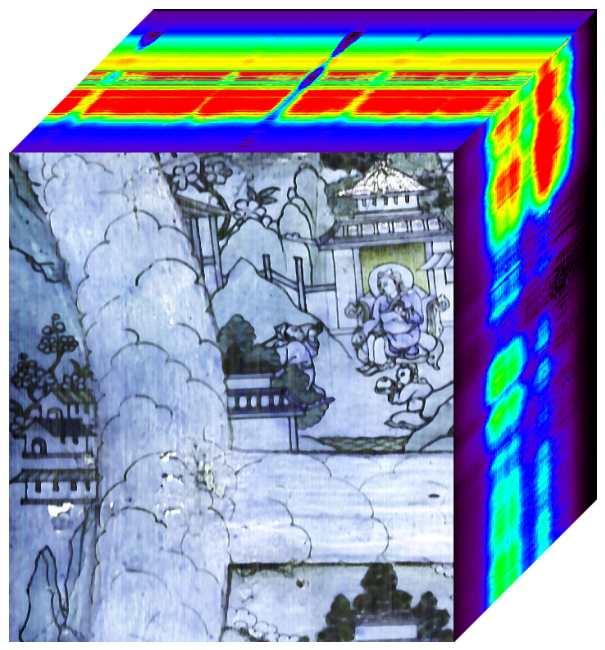
Hyperspectral imaging was performed on Potala Palace mural samples as a close-range acquisition demonstration. The reconstructed data cube preserves clear spatial texture together with wavelength-dependent information. Because neither an authenticated pigment reference spectral library covering the relevant materials and measurement conditions nor independent Raman or X-ray fluorescence confirmation was available, reliable pigment identification was beyond the scope of this study. The measurements are therefore presented as a demonstration of close-range spatial–spectral data acquisition rather than definitive pigment identification. A representative reconstructed hyperspectral data cube and the on-site measurement setup are shown in Figure 15 and Figure 16. The measured system performance metrics are summarized in

Table 10. Summary of measured system performance metrics.

Metric	Measured Value
Object-space sampling interval	82.4 μm/pixel
Spectral range	400–1000 nm
Spectral sampling interval	4.85 nm
Spectral resolution (SRF FWHM)	6.3 nm
Wavelength calibration accuracy	<0.9 nm
Expanded wavelength uncertainty	0.72 nm, k = 2
MTF at Nyquist	0.34
Residual smile	≤0.3 pixels
Residual keystone	≤0.3 pixels
Mean/peak SNR	339/613
Residual radiometric nonuniformity	0.71%
Maximum wavelength drift at 550 nm	0.42 nm

.

8. Discussion

A finite-conjugate VNIR pushbroom hyperspectral camera was designed and experimentally characterized for close-range cultural heritage imaging. At the nominal working distance of 404 mm, the system provides a slit-direction object-space sampling interval of approximately 82.4 μm/pixel. With a scan speed of 23.15 mm/s and a line rate of 275 Hz, the corresponding scan-direction sampling interval is approximately 84.2 μm, providing closely matched spatial sampling in the two image dimensions.

An integrated design, calibration, and characterization workflow was established for the specified finite-conjugate configuration. The measured end-to-end MTF was 0.34 at the effective Nyquist frequency, the mean SRF FWHM was approximately 6.3 nm, and the maximum absolute wavelength residual was below 0.90 nm. Residual smile and keystone errors were below 0.3 pixel, residual radiometric nonuniformity was 0.71%, and the wavelength-averaged SNR was 339. Repeated measurements and temperature stability testing were additionally used to evaluate the reproducibility of the principal calibration results.

The measurements of Potala Palace mural samples demonstrated the acquisition of spatially detailed and wavelength-resolved data under the specified close-range geometry. Because the material compositions were not independently verified using authenticated pigment standards or complementary analytical methods, the results are interpreted as a spatial–spectral documentation demonstration rather than definitive pigment identification.

Table 11. A comparison of representative commercial VNIR hyperspectral cameras and the system developed in this work [15,16,17,18,19].

System	Spectral Range/nm	Spectral Resolution/nm	Spatial Pixels	SNR	Working Distance	Application
HySpex VNIR-1800	400–1000	N.R.	1800	>180 (unbinned); >255 (2× binning)	A few centimeters–∞	Airborne, outdoor, and laboratory imaging
Headwall MV.C VNIR	400–1000	N.R.	1024	N.R.	Lens-dependent minimum (100–150 mm)	Industrial and machine vision inspection
Specim IQ	400–1000	7	512	>400 (peak)	150 mm–∞	Portable field and laboratory imaging
Specim FX10	400–1000	5.5	1024	N.R.	Lens-dependent	Industrial inspection and laboratory imaging
Resonon Pika L	400–1000	2.7	900	N.R.	Lens-dependent	Laboratory, field and airborne imaging
This work	400–1000	6.3	680 (three-pixel binning)	339 (mean) 613 (peak)	404 mm	Close-range mural imaging

N.R., not reported. Spectral resolution refers to the manufacturer-reported FWHM; HySpex reports spectral sampling rather than FWHM. Manufacturer-reported SNR values and the measured values in this work were obtained under different conditions and are therefore not directly comparable.

places the developed camera in the context of representative commercial VNIR hyperspectral systems. Several commercial cameras support close-up imaging through focusable or interchangeable lenses; therefore, short working distance alone is not claimed as the principal advantage of this work. The distinction lies in the end-to-end characterization of optical performance, matched object-space sampling in the slit and scan directions, wavelength and geometric calibration, and radiometric performance at a defined finite-conjugate geometry.

Wavelength calibration accuracy and the end-to-end MTF were omitted from Table 11 because comparable values under specified finite-conjugate configurations are not publicly reported for most commercial systems. An independent commercial hyperspectral camera or laboratory spectrometer was not available for cross-instrument validation. The reported calibration results were therefore evaluated against the monochromator and calibrated integrating sphere rather than through direct inter-instrument comparison. Such independent validation will be included in future work.

9. Conclusions

A VNIR pushbroom hyperspectral camera was developed and characterized for cultural heritage imaging at a working distance of 404 mm. The finite-conjugate configuration provides matched sampling intervals of 82.4 μm/pixel in the slit direction and 84.2 μm in the scan direction at 23.15 mm/s and 275 Hz.

A design, calibration, characterization, and evaluation workflow was established, covering optical design, spectral and geometric calibration, radiometric calibration, relative reflectance conversion, scan synchronization, SNR evaluation, and temperature stability assessment. The end-to-end MTF at the effective Nyquist frequency was 0.34. The mean spectral sampling interval and SRF FWHM were 4.85 and 6.3 nm, respectively. The maximum absolute wavelength residual was below 0.90 nm, with an expanded uncertainty of 0.72 nm at k = 2. Residual smile and keystone errors were below 0.3 pixels, radiometric nonuniformity was 0.71%, and the mean and peak SNR values were 339 and 613, respectively.

The measurements of Potala Palace mural samples demonstrated spatially detailed and wavelength-resolved data acquisition under close-range conditions. Because an authenticated pigment reference spectral library and independent Raman or X-ray fluorescence confirmation were unavailable, this experiment is presented as a spatial–spectral documentation demonstration rather than definitive pigment identification. The contribution is an experimentally validated workflow linking finite-conjugate design, object-space sampling, scan synchronization, and calibration performance at a defined close-range geometry.

References

- Yu, K.; Hou, Y.; Fu, Y.; Ni, W.; Zhang, Q.; Wang, J.; Peng, J. Automatic labeling framework for paint loss disease of ancient murals based on hyperspectral image classification and segmentation. Herit. Sci. 2024, 12, 192. [Google Scholar] [CrossRef] [Scilit]
- Delaney, J.K.; Thoury, M.; Zeibel, J.G.; Ricciardi, P.; Morales, K.M. Visible and infrared imaging spectroscopy of paintings and improved reflectography. Herit. Sci. 2016, 4, 6. [Google Scholar] [CrossRef] [Scilit]
- Delaney, J.K.; Walmsley, E.; Berrie, B.H.; Fletcher, C.F. Scientific Examination of Art—Modern Techniques in Conservation and Analysis; The National Academies Press: Washington, DC, USA, 2005; pp. 120–136. [Google Scholar]
- Kleynhans, T.; Patterson, C.M.S.; Dooley, K.A.; Messinger, D.W. An alternative approach to mapping pigments in paintings with hyperspectral reflectance image cubes using artificial intelligence. Herit. Sci. 2020, 8, 84. [Google Scholar] [CrossRef] [Scilit]
- Pei, Z.; Huang, Y.M.; Zhou, T. Review on Analysis Methods Enabled by Hyperspectral Imaging for Cultural Relic Conservation. Photonics 2023, 10, 1104. [Google Scholar] [CrossRef] [Scilit]
- Li, G.H.; Chen, Y.; Sun, X.J.; Duan, P.Q.; Lei, Y.; Zhang, L.F. An automatic hyperspectral scanning system for the technical investigations of Chinese scroll paintings. Microchem. J. 2020, 155, 104699. [Google Scholar] [CrossRef] [Scilit]
- Delaney, J.K.; Zeibel, J.G.; Thoury, M.; Littleton, R.; Palmer, M.; Morales, K.M.; de la Rie, E.R.; Hoenigswald, A. Visible and infrared imaging spectroscopy of Picasso’s Harlequin Musician: Mapping and identification of artist materials in situ. Appl. Spectrosc. 2010, 64, 584–594. [Google Scholar] [CrossRef] [Scilit] [PubMed]
- Dik, J.; Janssens, K.; Van Der Snickt, G.; van der Loeff, L.; Rickers, K.; Cotte, M. Visualization of lost painting by Vincent Van Gogh using synchrotron radiation based X-ray fluorescence elemental mapping. Anal. Chem. 2008, 80, 6436–6442. [Google Scholar] [CrossRef] [Scilit] [PubMed]
- Bacci, M.; Picollo, M. Non-destructive spectroscopic detection of cobalt (II) in paintings and glass. Stud. Conserv. 1996, 41, 129–135. [Google Scholar] [CrossRef] [Scilit]
- Clark, R.N.; Swayze, G.A.; Wise, R.A.; Livo, K.E.; Hoefen, T.M.; Kokaly, R.F.; Sutley, S.J. USGS Digital Spectral Library splib06a; U.S. Geological Survey Data Series 231; U.S. Geological Survey: Reston, VA, USA, 2007. [Google Scholar]
- Dunn, J.R.; Berrie, B.H.; Delaney, J.K.; Glinsman, L.D. The creation of Giotto’s Madonna and Child: New insights. In Facture; Yale Press: New Haven, CT, USA, 2015; Volume 2, pp. 2–17. [Google Scholar]
- Casini, A.; Bacci, M.; Cucci, C.; Lotti, F.; Porcinai, S.; Picollo, M.; Radicati, B.; Poggesi, M.; Stefani, L. Fiber optic reflectance spectroscopy and hyper-spectral image spectroscopy: Two integrated techniques for the study of the Madonna dei Fusi. Proc. SPIE 2005, 5857, 177–184. [Google Scholar] [CrossRef] [Scilit]
- Picollo, M.; Bacci, M.; Magrini, D.; Radicati, B.; Trumpy, G.; Tsukada, M.; Kunzelman, D. Modern white pigments: Their identification by means of noninvasive ultraviolet, visible, and infrared fiber optic reflectance spectroscopy. In Proceedings of the Conference Modern Paints Uncovered, London, UK, 16–19 May 2007; pp. 118–128. [Google Scholar]
- Hou, M.; Zhou, P.; Lv, S.; Hu, Y.; Zhao, X.; Wu, W.; He, H.; Li, S.; Tan, L. Virtual restoration of stains on ancient paintings with maximum noise fraction transformation based on hyperspectral imaging. J. Cult. Herit. 2018, 34, 136–144. [Google Scholar] [CrossRef] [Scilit]
- Specim, Spectral Imaging Ltd. Specim IQ Hyperspectral Camera: Data Sheet. Available online: https://www.specim.com/wp-content/uploads/2024/11/Specim-IQ-Datasheet-Long-08.pdf (accessed on 20 June 2026).
- Specim, Spectral Imaging Ltd. Specim FX10. Available online: https://www.specim.com/products/specim-fx10 (accessed on 20 June 2026).
- Headwall Photonics, Inc. MV.C VNIR Hyperspectral Imager. Available online: https://headwallphotonics.com/products/machine-vision/mv-c-vnir-hyperspectral-imager (accessed on 20 June 2026).
- Resonon Inc. Pika L Hyperspectral Imaging Camera. Available online: https://resonon.com/Pika-L (accessed on 20 June 2026).
- Norsk Elektro Optikk AS. HySpex VNIR-1800 Hyperspectral Camera. Available online: https://www.hyspex.com/hyspex-products/hyspex-classic/vnir-1800 (accessed on 20 June 2026).
Figure 1.
Optical layout.
Figure 2.
System overview, coordinate definition, and pushbroom reconstruction geometry.
Figure 3.
Simulated slit-direction MTF at full fields and wavelengths. (a) MTF@0.4 μm; (b) MTF@0.7 μm; (c) MTF@1.0 μm.
Figure 4.
Spot diagrams for different wavelengths and fields of view: (a) 0.4 μm; (b) 0.7 μm; (c) 1.0 μm.
Figure 5.
Sequential workflow for spatial, spectral, and radiometric alignment.
Figure 6.
Smile test result.
Figure 7.
Keystone test result.
Figure 8.
The wavelength-dependent spectral radiance calibration coefficient a(λ) of the VNIR hyperspectral camera.
Figure 9.
Measured MTF diagram.
Figure 10.
Measured normalized spectral response functions across the VNIR range.
Figure 11.
Wavelength calibration curve and pixel-to-wavelength mapping.
Figure 12.
N = The normalized end-to-end spectral responsivity of the VNIR hyperspectral camera derived from the inverse spectral radiance calibration coefficient.
Figure 13.
SNR distribution over the retained 400–1000 nm spectral channels.
Figure 14.
The measured temperature and center wavelength drift of the 550 nm monochromatic response during the 20–10–30 °C set-point cycle.
Figure 15.
Representative reconstructed hyperspectral data cube of mural sample.
Figure 16.
On-site measurement setup for mural imaging.