Single-Scale EMA Latent Memory for Strictly Causal Dense Arm-Motion Recognition from Multi-Channel sEMG

Featured Application

This study provides a controlled strictly causal benchmark for dense pointwise sEMG recognition research in rehabilitation interfaces, prosthetic control, and human–machine interaction. It evaluates the trade-offs among causal context use, transition sensitivity, and model-level full-buffer efficiency; it does not validate incremental, real-time, embedded, or end-to-end deployment.

Abstract

Strictly causal dense arm-motion recognition from surface electromyography (sEMG) requires past context without future samples. We evaluated single-scale exponential moving average (EMA) latent memory as a lightweight causal temporal mechanism under a controlled, matched design. Causal CNN, causal CNN–Transformer (CT), and causal CNN with EMA memory (CEMA) were tested on a 30-subject, eight-channel, seven-class dataset in five subject-independent folds. At 300, 500, and 800 ms, five deterministic seeds were averaged within-fold before inference. CEMA accuracy exceeded CNN accuracy by 9.105, 9.313, and 9.657 percentage points, respectively (all Holm-adjusted paired-t p < 0.001). CEMA–CT differences were +0.209, −0.240, and −0.715 points, respectively; confidence intervals included zero, and directions varied across seeds. With parameters frozen, resetting memory at the current-window start reduced CEMA accuracy by 10.928–17.009 points. CEMA–CT B100 recall differences were −4.97, −12.84, and −16.54 points, respectively, whereas absolute-delay differences were 6.79, 7.71, and 6.94 ms, respectively, all below 8 ms. At 300 ms, CEMA used 6968 parameters and 0.751 M MACs, 48.0% fewer MACs than CT; CT required 2.31× CEMA’s full-buffer host-wall time. CEMA offers a favorable average accuracy–efficiency trade-off, although CT remains more responsive at transitions. Timing reflects full-buffer host inference only, not incremental, embedded, or end-to-end deployment.

1. Introduction

1.1. Dense Pointwise sEMG Recognition as a Strictly Causal Sequence Problem

Surface electromyography (sEMG) provides a non-invasive measure of muscle activation. Early pattern-recognition methods for multifunction myoelectric control demonstrated the practical value of translating muscle activity into movement commands [1]. Recent reviews have described myoelectric prosthetic-hand control, sEMG challenges in prosthetic applications, neural-information extraction, and clinical perspectives for myoelectric prostheses [2,3,4,5]. In rehabilitation and human–machine interaction, however, the accurate classification of isolated signal segments is not sufficient. A recognition system must also produce coherent labels as muscle activation emerges, actions change, and the user returns to rest. Strictly causal dense pointwise recognition, therefore, involves a balance among discrimination, temporal consistency, response timing, and the information available at the moment each prediction is made.

Most sEMG pattern-recognition studies assign a single label to a fixed analysis window and evaluate each window independently. Public benchmark datasets have improved the reproducibility of this fixed-window setting for non-invasive robotic-hand control [6], while CNN-based models and transfer-learning methods offer complementary ways to learn or reuse window-level representations [7,8]. Dense pointwise recognition poses a different challenge because every valid sample within the current window must receive a label. Here, “dense” refers to pointwise predictions within each current window, whereas model updates occur at the specified window stride. This distinction matters near action boundaries: a few isolated label changes can fragment the output, but an unusually low transition count may also indicate that true transitions have been delayed or missed. Neither aggregate accuracy nor transition count alone is sufficient to characterize this behavior.

Reliable comparison is further complicated by variation across subjects, recording sessions, electrode placements, and tasks. A recent survey identifies these factors as major sources of generalization difficulty in sEMG-based hand-gesture recognition [9]. Few-shot learning, transfer learning, and unsupervised domain adaptation address different forms of limited supervision and recording-condition shift [10,11,12], while large-scale multi-user zero-shot modeling and recent sEMG architecture-design work extend this perspective [13,14]. Performance also depends on segmentation choices [15], feature representation [16], and classifier design for cross-individual recognition [17]. These considerations motivate the use of subject-independent folds, a shared pre-processing and optimization protocol, and a clear separation between internal temporal modeling and output post-processing. Under such controlled conditions, a matched temporal-module comparison is more informative than a direct comparison, with heterogeneous results reported across prior studies.

1.2. Temporal Context, Causality, and Matched Model Comparison

CNNs are effective at extracting local temporal patterns and cross-channel structures from sEMG signals [18]. More elaborate variants extend this capability through multi-scale fusion, channel attention, or gated temporal convolution [19,20]. Even so, simply increasing the input-buffer length does not determine how information from different time points is retained, weighted, or integrated. Local convolutional encoding is, therefore, an important component of temporal representation, but it does not by itself provide an explicit mechanism for maintaining historical context.

Sequence models address this limitation through several mechanisms. Temporal convolutions can provide sequence-modeling baselines [21,22], while attention-based transfer models have been used for electromyographic gesture estimation [23], and real-time motor-unit decoding illustrates an alternative signal-processing path [24]. Structured state-space models use state recursions [25,26,27], and EMA-like or retention mechanisms combine recurrent updates with gated attention or parallel/recurrent formulations [28,29]. Transformer-based architectures have been applied to conventional and high-density sEMG gesture recognition [30,31,32]. Related studies have also combined CNNs with Vision Transformers or used Transformer-based models for continuous and deployable sEMG estimation [33,34,35]. Recent studies have further considered noise resilience, time-varying feature enhancement, and wearable high-density sensing to challenge sEMG recognition settings [36,37,38]. Although these approaches differ in their representational flexibility, memory organization, and implementation cost, their central distinction lies in how past information is stored, weighted, and combined.

Recent neural sequence architectures have already incorporated EMA-like state updates in richer mechanisms: Moving Average Equipped Gated Attention (MEGA) couples multi-dimensional damped EMA with gated attention, whereas Retentive Network (RetNet) uses a retention mechanism with parallel, recurrent, and chunkwise-recurrent formulations [28,29].

The present study does not claim to introduce EMA, a new attention architecture, or a general state-space model. Instead, it examines whether the proposed Causal CNN + single-scale EMA latent memory (CEMA) model can retain useful causal encoder history for dense sEMG recognition through a deliberately constrained shared-scalar EMA state. The CEMA temporal path is restricted to one temporal scale and does not perform content-dependent attention. It is, therefore, positioned as a compact and interpretable point within the broader temporal-modeling design space.

A causal Transformer provides a relevant and more flexible comparator for this question. We, therefore, compared three matched models: a Causal Convolutional Neural Network (CNN), a Causal CNN–Transformer (CT), and CEMA. To isolate the effect of the temporal module, the three models shared the same causal CNN encoder, dense decoder, optimizer, subject folds, and validation-based checkpoint-selection rule. CT served as a matched temporal comparator rather than as the proposed architecture, and differences between CEMA and CT should not be attributed solely to self-attention.

Here, causality is defined as an end-to-end restriction on information access. A prediction at time t may depend only on raw or derived signal samples available no later than t. A causal mask inside the neural network is, therefore, insufficient if pre-processing has already introduced future information into an earlier representation. To enforce strict causality throughout the pipeline, we use forward-only filtering, zero neural look-ahead, history-buffered current-window inputs, and loss and evaluation restricted to the final current window. Available context, cold-start duration, update interval, and future look-ahead are reported separately because they describe different aspects of temporal availability and response timing.

1.3. Single-Scale EMA Latent Memory and Study Scope

Let $z_{\mathcal{l}}$ denote the causal feature produced by the shared CNN encoder. A single learned scalar $\alpha \in (0,1)$ recursively combines the current feature with the previous latent state. The resulting state is fused with the current feature before dense decoding. This design provides one explicit temporal scale while preserving a direct path for current evidence. It should, therefore, be understood as a compact causal latent-state accumulator rather than as a multi-scale memory bank or an attention mechanism.

The principal contribution of this study is a carefully controlled evaluation of a lightweight single-scale EMA latent memory mechanism for strictly causal dense sEMG recognition, rather than the introduction of a fundamentally new sequence-modeling architecture. CNN, CT, and CEMA share the same causal encoder, dense decoder, pre-processing, subject-independent folds, optimization, and checkpoint-selection procedure, which allows the temporal module to be examined under matched conditions. The evaluation asks whether CEMA benefits from informative historical content, how its pointwise recognition performance relates to boundary sensitivity, and whether it can approach a matched causal Transformer with a lower model cost. These questions are addressed through trained and frozen-checkpoint memory ablations, window-internal and stream-level boundary analyses, causal smoothing controls, and efficiency measurements. The complete $W=100$ ms context curve (100–1100 ms) is reported descriptively using seed 0, whereas 300, 500, and 800 ms serve as the primary context anchors for five-seed inference. A seed-0 $W=10$ ms feasibility pilot is reported separately in Supplementary Methods S1 and Supplementary Table S5 and is not used for primary inference or deployment claims.

2. Materials and Methods

2.1. Data, Labels, and Subject-Independent Splits

We used the public MyoelectricData example dataset distributed with the Myoelectric Control Development Toolbox [39]. The dataset comprises 720 matched signal–label recording pairs from 30 subjects, with 24 recordings per subject. Each signal recording contains eight sEMG channels sampled at 3000 Hz, and the corresponding label file provides pointwise annotations for seven arm-motion classes: Hand Open, Hand Close, Wrist Flexion, Wrist Extension, Supination, Pronation, and Rest.

Evaluation followed a five-fold subject-independent design. The 30 subject identifiers were shuffled once using random seed 0 and divided into five non-overlapping test groups of six subjects each. For each fold, the first four subjects of the next group in cyclic order were used for validation, while the remaining 20 subjects formed the training set. Training, validation, and test subjects were, therefore, mutually disjoint within every fold. The test sets for folds 1–5 were {1, 4, 6, 11, 18, 19}, {8, 15, 21, 26, 27, 30}, {3, 5, 7, 20, 22, 24}, {10, 12, 16, 17, 23, 29}, and {2, 9, 13, 14, 25, 28}, respectively, ensuring that every subject appeared in the test set exactly once. Checkpoints and validation-controlled parameters were selected using only the training and validation subjects. The held-out test subjects were evaluated only after model selection had been completed.

After pre-processing, the dense label sequences had an effective temporal resolution of 1000 Hz. The five held-out subject folds, rather than individual labeled time points, served as the independent statistical units for uncertainty estimation. Across the pooled test predictions, the proportions of the seven classes ranged from 13.869% to 14.641%, with Rest accounting for 14.441%. This near-balanced distribution supports the use of Macro-F1 as a class-balanced complement to accuracy and reduces concern that the aggregate results were dominated by a single majority class.

2.2. Strictly Causal Pre-Processing and Current-Window Evaluation Protocol

Raw sEMG recordings were sampled at 3000 Hz and filtered using a fourth-order 10–400 Hz Butterworth band-pass filter implemented with scipy.signal.sosfilt [40]. Filtering was applied once to each complete recording in the forward direction, with the filter state initialized to zero at recording onset. No scipy.signal.filtfilt or other bidirectional operation was used, and startup-transient samples were retained. Label intervals were reconstructed from the annotated one-based data_indx start positions, with each interval ending immediately before the next annotated start and the final interval extending for 3 s. Filtering preceded label-based sample selection so that the causal filter state continued through unlabeled regions. After filtering, only samples belonging to the seven target classes were retained. Signals and labels were then subsampled using identical zero-based indices (0, 3, 6, …), yielding pointwise-aligned sequences at 1000 Hz, corresponding to a temporal resolution of 1 ms. No amplitude normalization, standardization, or subject-level scaling was applied.

In the primary protocol, each block had a duration of $W=100$ ms. Each input consisted of m historical blocks followed by one final current block, with $m=0,\dots ,10$ and consecutive inputs advanced by one block (stride_windows = 1). Historical blocks provided context only, whereas the training loss and all primary evaluation metrics were computed exclusively over the final current block. The total available causal context was, therefore, $(m+1)W$, the update interval was $W$, and informational future look-ahead was 0 ms; no prediction depended on signal samples occurring later than the predicted time point. The evaluated implementation used full-buffer inference, in which the complete current block was accumulated before one forward pass produced all dense predictions for that block. Current-window buffering, therefore, introduced no waiting for the final sample and up to $W-1$ ms for the first sample, corresponding to 0–99 ms for $W=100$ ms and 0–9 ms for $W=10$ ms, excluding model-execution time. This buffering delay is distinct from the update interval and from end-to-end system latency, which was not measured. To ensure that all context settings were evaluated at identical current-window positions, candidate windows were sampled every 100 ms from a common eligible region beginning 1600 ms after recording onset. This excluded the first 16 candidate windows from each recording, corresponding to 1.878% of the otherwise eligible $m=0$ windows. These samples remained part of causal filtering but were not used as evaluation windows. Each buffered input was drawn entirely from a single recording, so neither the historical context nor the current block crossed a recording boundary.

A separate seed-0 $W=10$ ms descriptive feasibility pilot, including its separate block protocol and results, is reported in Supplementary Methods S1 and Supplementary Table S5. It is not pooled with the $W=100$ ms primary-anchor analysis and does not establish seed-robust superiority, online execution, or end-to-end latency.

2.3. Matched Causal Model Architectures

All three models shared the same input representation, causal CNN encoder, dense decoder, subject-independent folds, optimizer, and checkpoint-selection protocol. As shown in

Table 1. Matched model architectures and causality audit.

Component	CNN	CT	CEMA
Input	8-channel sEMG	8-channel sEMG	8-channel sEMG
Encoder	Two causal Conv1D (8→32→16)	Two causal Conv1D (8→32→16)	Two causal Conv1D (8→32→16)
Temporal module	Identity path	Two causally masked Transformer layers	Single-scale causal EMA latent memory
Decoder	Upsampling classification head	Upsampling classification head	Upsampling classification head
Output	7-class dense logits	7-class dense logits	7-class dense logits
Learnable parameters	6407	12,967	6968

Note. sEMG, surface electromyography; CNN, causal convolutional neural network; CT, causal CNN–Transformer; EMA, exponential moving average; CEMA, causal CNN with EMA memory; Conv1D, one-dimensional convolution.

, their sole architectural difference was the temporal path between the encoder and decoder: an identity mapping in CNN, a causally masked Transformer in CT, and the single-scale EMA latent memory module in CEMA. This matched design was intended to isolate the effect of the temporal module while holding local feature extraction, dense decoding, data splits, optimization, and model-selection procedures fixed. CT, therefore, served as a matched temporal comparator rather than as a comparator of self-attention alone, because the Transformer block also contains other operations.

The shared encoder received an eight-channel sEMG sequence and contained two one-dimensional causal convolutional layers with channel progression 8→32→16. Each layer used a kernel size of 8, a stride of 2, seven-sample left padding, and zero right padding, which resulted in an overall downsampling factor of 4. Each encoder layer followed the sequence Conv1D, ReLU, and timewise LayerNorm over the channel dimension. Thus, every latent position depended only on the current and preceding input samples. Using the same encoder across all three models ensured identical local feature extraction and temporal downsampling.

The models differed in how the encoded latent sequence was processed. In CNN, the encoder output was passed directly to the decoder through an identity path, without an additional temporal-context module. In CT, fixed sinusoidal positional encoding was added to the latent sequence before it was processed by two PyTorch Transformer encoder layers [41]. Each layer used a model dimension of $d=16$, four attention heads, a feed-forward dimension of 64, dropout of 0.1, ReLU activation, post-norm ordering (norm_first = False), residual connections, and the standard LayerNorm configuration. A strict upper-triangular Boolean mask prevented attention to future latent positions. CT served as a matched temporal-context comparator, and its comparison with CEMA, therefore, reflected the complete Transformer block rather than self-attention alone. The positional encoding was preallocated for 50,000 latent positions.

In CEMA, temporal context was represented by a recursively updated causal state. A single learned decay parameter was shared across all 16 latent dimensions. At each latent position, the current encoder feature and the corresponding EMA-memory state were combined through a 1 × 1 fusion layer, followed by a residual connection and LayerNorm. The residual path preserved the current local representation, while the EMA state carried compressed information from preceding latent positions.

All three temporal paths were connected to the same dense decoder. A shared 1 × 1 Conv1D classifier mapped the 16-dimensional latent representation to seven class logits. These logits were upsampled to the original input-sample resolution using repeat-interleave with a factor of 4, producing dense predictions for the seven classes. Training loss and all primary evaluation metrics were computed only over the final current window. Because the encoder, temporal modules, and decoder used no future information, all three models had a future look-ahead of 0 ms.

The CNN, CT, and CEMA models contained 6407, 12,967, and 6968 learnable parameters, respectively. The parameter counts were not artificially equalized because the temporal modules had inherently different structures. Instead, comparison fairness was maintained through the shared encoder and decoder, identical subject-independent folds, optimizer settings, training procedure, and checkpoint-selection criterion. CEMA contained additional state-fusion parameters that were absent from the CNN identity path. The history-removal and latent-masking ablations were, therefore, used to assess whether its performance gains arose from informative historical content rather than from the additional fusion parameters alone.

2.4. Single-Scale EMA Latent Memory Module

For the causal latent sequence $Z=\left[z_0,\dots ,z_{L-1}\right]=E_{{\theta }_e}\left(X\right)$ produced by the shared encoder, with $z_{\mathcal{l}}\in {\mathbb{R}}^d$ and $d=16$, the proposed temporal module maintains a single recurrent EMA state across latent time. Because the encoder downsamples the input by a factor of four, one latent step corresponds to 4 ms. A trainable scalar $\gamma$, shared across all latent dimensions and distinct from the encoder parameters ${\theta }_e$, is mapped to a valid EMA coefficient through $\alpha =\mathrm{sigmoid}\left(\gamma \right)\in \left(0,1\right)$. The memory state is initialized as $h_{-1}=0$ at the beginning of each buffered sequence.

At latent index $\mathcal{l}$, the state is updated as

$$h_{\mathcal{l}}=\alpha z_{\mathcal{l}}+\left(1-\alpha \right)h_{\mathcal{l}-1}$$

(1)

where $h_{\mathcal{l}}\in {\mathbb{R}}^d$ is the EMA state and $z_{\mathcal{l}}$ is the current latent feature. This update is strictly causal because it depends only on the current feature and the preceding state. The same coefficient $\alpha$ is applied to all latent dimensions.

With zero initialization, Equation (1) can be expanded as

$$h_{\mathcal{l}}={\displaystyle {\sum }_{j=0}^{\mathcal{l}}}\alpha {\left(1-\alpha \right)}^j{z}_{\mathcal{l}-j}, w_j=\alpha {\left(1-\alpha \right)}^j$$

(2)

where $j$ denotes the lag in latent steps and $w_j$ is the corresponding lag weight. The resulting kernel depends only on temporal lag and defines a single shared exponential timescale; it is neither content-dependent attention nor a multi-scale memory bank.

The relative EMA kernel weight at lag $q$ is ${\displaystyle \frac{w_q}{w_0}}={(1-\alpha )}^q$. We define the continuous 5–relative-weight horizon as

$${\tau }_{\mathrm{5\%}}=4{\displaystyle \frac{\mathrm{l}\mathrm{n}\left(0.05\right)}{\mathrm{l}\mathrm{n}(1-\alpha )}}\mathrm{m}\mathrm{s}$$

(3)

where ${\tau }_{5\mathrm{\%}}$ denotes the lag at which the EMA kernel weight decreases to 5% of its zero-lag value. The factor of 4 ms follows from the encoder’s four-fold temporal downsampling.

Before dense decoding, the current latent feature and its EMA state are fused as

$$u_{\mathcal{l}}=\mathrm{LN}\left(z_{\mathcal{l}}+W_f\left[z_{\mathcal{l}};h_{\mathcal{l}}\right]+b_f\right)$$

(4)

where $u_{\mathcal{l}}$ is the fused latent feature, $W_f$ and $b_f$ are the learnable 1 × 1 fusion-projection parameters, $\left[z_{\mathcal{l}};h_{\mathcal{l}}\right]$ denotes concatenation along the channel dimension, and LN denotes LayerNorm. The residual term $z_{\mathcal{l}}$ preserves current local evidence, while the EMA state supplies accumulated historical context.

The shared decoder $D_{\varphi }$, parameterized by $\varphi$, maps the fused latent sequence $U=\left[u_0,\dots ,u_{L-1}\right]$ to dense class probabilities:

$$p_t=\mathrm{softmax}\left({D_{\varphi }\left(U\right)}_t\right)$$

(5)

where $p_t$ is the class-probability vector at input-time index $t$. Let $I_{\mathrm{cur}}$ denote the indices of the final current window and $y_t$ the corresponding ground-truth label. The training objective is

$$\mathrm{L}=-{\displaystyle \frac{1}{\left|I_{\mathrm{cur}}\right|}}\sum _{t\in I_{\mathrm{cur}}}\log p_t\left[y_t\right]$$

(6)

Historical blocks, therefore, provide context only, whereas loss computation and all primary evaluation metrics are restricted to the final current window. During inference, the encoder first produces $Z$; the EMA state is then updated recursively using Equation (1), fused with the current latent feature using Equation (4), and decoded using Equation (5). Only predictions indexed by $I_{\mathrm{cur}}$ are retained.

Under incremental execution, the EMA recurrence requires $O\left(d\right)$ persistent state and $O\left(d\right)$ arithmetic per latent step, while the fusion projection requires $O\left(d^2\right)$ operations. These properties establish the mathematical feasibility of stateful incremental execution; however, the timing experiments reported in Section 3.4 evaluate full-buffer recomputation rather than an optimized streaming implementation.

2.5. Training and Model-Selection Configuration

2.5.1. Single-Seed Analyses

All three models were trained using the Adam optimizer with a learning rate of 0.001, ${\beta }_1=0.9$, ${\beta }_2=0.999$, $\epsilon ={10}^{-8}$, zero weight decay, and amsgrad = False. No learning-rate scheduler was used. Training was limited to 500 epochs, with early stopping based on validation accuracy and a patience of five epochs. The training and evaluation batch sizes were, respectively, 64 and 128 for input lengths below 800 samples, 48 and 96 for lengths from 800 to 1599 samples, and 32 and 64 for lengths of at least 1600 samples. A separate model was trained for each architecture × subject-fold × context combination. CNN, CT, and CEMA followed the same pre-processing pipeline, subject-independent folds, objective function, evaluation metrics, optimizer settings, and checkpoint-selection procedure. Training minimized the pointwise cross-entropy defined in Section 2.4, with supervision and loss computation restricted to the valid indices of the final current window, $I_{\mathrm{c}\mathrm{u}\mathrm{r}}$; historical blocks provided context only.

Model selection and early stopping relied exclusively on the validation set. The held-out test subjects were not used for parameter updates, early stopping, or checkpoint selection and were evaluated only after model selection had been completed. Validation pointwise accuracy was the sole criterion: the checkpoint was updated only when validation accuracy strictly improved, and training stopped after five consecutive epochs without improvement. The retained checkpoint contained the model state_dict only, without optimizer or scheduler state. For the complete-context sweep and auxiliary analyses, seed 0 was applied to Python, NumPy, PyTorch, and all CUDA devices, although deterministic algorithms were not explicitly enforced.

This single-seed configuration generated the complete $W=100$ ms, m$=$0–10 context curve and the auxiliary trained-history and $W=10$ ms analyses, and it supplied the checkpoints used by the seed-0 smoothing analyses. Unless explicitly identified as part of the multi-seed retraining below, these results represent one fit per architecture × subject-fold × context combination and, therefore, do not estimate training-seed variability.

2.5.2. Deterministic Multi-Seed Anchor Analyses

For the primary multi-seed analysis, subject assignments were fixed using split seed 0, and CNN, CT, and CEMA were each trained with seeds 0, 1, 2, 3, and 4 at $m=2, 4$ and 7 (300, 500, and 800 ms, respectively) across the five held-out subject folds. This yielded $5\times 3\times 3\times 5=225$ completed training runs. All repeats used the same cached causal pre-processing, common eligible evaluation region, optimizer, early-stopping rule, validation-accuracy checkpoint selection, and current-window-only objective specified above; only training stochasticity was varied.

Each training seed controlled Python, NumPy, PyTorch, and all CUDA generators, model initialization, a dedicated mini-batch shuffling generator, dropout, and other stochastic operations. PyTorch deterministic algorithms and deterministic cuDNN execution were enabled; cuDNN benchmarking and TF32 were disabled; float32 matrix-multiplication precision was set to highest; CUBLAS_WORKSPACE_CONFIG was set to 4096:8; and pointwise logits and labels were flattened before cross-entropy computation to avoid a nondeterministic three-dimensional CUDA NLL path. Runs used Windows 10 build 26200, Python 3.11.14, PyTorch 2.12.0.dev20260218+cu128, CUDA 12.8, cuDNN 9.10.2, NumPy 2.2.1, and an NVIDIA GeForce RTX 5060 Ti. Environment settings and source hashes were retained with the analysis records.

2.6. Evaluation Metrics, Boundary Analyses, Smoothing Controls, and Diagnostic Ablations

2.6.1. Window-Internal Boundary Evaluation and Smoothing Controls

Accuracy was the primary pointwise metric, with Macro-F1 used as a complementary class-balanced measure. Accuracy was defined as the proportion of retained current-window time points assigned the correct label, whereas Macro-F1 was the unweighted mean of the seven class-specific F1 scores. Both metrics included all valid time points in the final current window. Event-level exclusions, therefore, did not affect accuracy, Macro-F1, or the classwise metrics. The five held-out subject folds, rather than individual time points, served as the statistical units for summary and uncertainty estimation.

Boundary events were defined as label changes within each evaluated 100 ms current window. The reference- and predicted-boundary sets were

$$B^{true}=\{t\in \left\{1,\dots ,99\right\}:y_t\ne y_{t-1}\}$$

(7)

and

$$B^{pred}=\{t\in \left\{1,\dots ,99\right\}:{\widehat{y}}_t\ne {\widehat{y}}_{t-1}\}$$

(8)

respectively. Thus, only adjacent sample pairs within the current window were eligible. A physical transition between the sample immediately preceding the current window and its first sample was excluded from event accounting, although all current-window samples remained included in the pointwise metrics. Boundary events were evaluated separately within each current window, without cross-window stitching or event credit across window boundaries. $B_{50}$, which required one-to-one predicted-to-reference matching within $\pm 50 \mathrm{m}\mathrm{s}$, was used as the primary localization-sensitive endpoint. $B_{100}$ was retained as a permissive within-window coverage audit. Because eligible boundary positions ranged from 1 to 99 ms, the maximum separation between any two candidates within a window was 98 ms.

Boundary precision was the proportion of predicted boundaries matched to a reference boundary, and boundary recall was the proportion of reference boundaries successfully matched. Boundary F1 was their harmonic mean, while the missed-transition rate was the proportion of reference boundaries left unmatched. Unmatched predicted boundaries were counted as false transitions. For each tolerance, all admissible reference–prediction pairs were ordered by absolute temporal offset, followed by the reference-boundary index and predicted-boundary index. Greedy one-to-one matching then accepted a pair only when neither boundary had previously been assigned. This procedure prioritized the smallest absolute offset and used earlier indices for deterministic tie-breaking. Matched-boundary delay was reported as the absolute temporal distance between matched predicted and reference boundaries. Signed delay was also calculated as prediction time minus reference time, with positive values indicating later predictions. False transitions were reported per 1000 retained current-window output points. A stable flip was defined as a predicted-label change between adjacent points whose ground-truth labels were unchanged, and its rate was reported per 1000 eligible ground-truth-stable adjacent pairs.

Post hoc causal smoothing controls were evaluated for the raw CNN and CT outputs at $m=2, 4$, and 7, corresponding to 300, 500, and 800 ms of available context, respectively. Candidate windows for causal-median-probability and majority-label smoothing were 20, 50, 100, and 200 ms. Candidate coefficients for causal EMA probability smoothing were α = 0.2, 0.5, and 0.8, with lower values producing stronger smoothing. Smoothing state was maintained across contiguous current windows within the same recording and reset at recording boundaries or temporal gaps. For each model × context × fold × smoothing family, the parameter was selected using validation accuracy. Ties were resolved first by higher validation Macro-F1 and then by the least aggressive smoothing setting. Only the validation-selected parameter was applied to the held-out test subjects. No output post-processing was applied to CEMA.

2.6.2. Stream-Level Boundary Sensitivity Analysis

To assess sensitivity to the exclusion of current-window joins, a stream-level boundary evaluation was performed with the 225 saved deterministic multi-seed checkpoints described in Section 2.5.2; no model was retrained. For every CNN, CT, and CEMA checkpoint at 300, 500, and 800 ms, truth and predicted labels from the 100 ms current windows were ordered chronologically by subject and original recording. Consecutive windows were stitched only when their source positions were exactly contiguous within the same subject and recording. The final sample of the preceding window and the first sample of the following window then formed an eligible adjacent pair. No adjacency, event match, or prediction sequence crossed a recording or subject boundary.

Within each reconstructed recording, reference and predicted boundaries were defined by every adjacent-sample label change, including changes at valid window joins. B50 and B100 used the same greedy closest one-to-one matching rule as the window-internal analysis, applied without allowing matches between recordings. Precision, recall, F1, signed and absolute matched-boundary delay, missed-transition rate, false transitions per 1000 retained output points, and stable-flip rate were recalculated. Pointwise accuracy and Macro-F1 were unchanged because both boundary accounting modes used the same output samples. Only saved prediction windows were stitched for event accounting; model inference remained full-buffer. This analysis, therefore, evaluates stream-level boundary sensitivity and does not validate incremental, embedded, real-time, or deployment execution.

2.6.3. Frozen-Checkpoint Diagnostic Memory Ablation

A frozen-checkpoint diagnostic ablation was performed with all 75 CEMA checkpoints from the five-seed primary-anchor experiment (five seeds × three contexts × five folds). Every checkpoint was loaded in evaluation mode, all parameters were frozen, and no optimizer, backpropagation, or retraining was used. Three inference conditions were evaluated: (1) normal chronological memory, the original CEMA forward pass over the complete history-plus-current buffer; (2) reset-at-current-window, in which the EMA state was initialized to zero at the start of the current 100 ms window and recomputed only over the current latent features; and (3) zero-memory branch, in which the memory tensor entering fusion was replaced by zeros.

For both interventions, the full input buffer and causal encoder outputs were retained. Reset-at-current-window–preserved within-window EMA recurrence, whereas zero-memory retained the direct current-feature path, fusion weights and bias, normalization, and decoder. The normal implementation was audited against the original checkpoint forward pass and reproduced its logits, predictions, accuracy, and Macro-F1. Resetting or zeroing memory can introduce distribution shift, and the causal encoder can still transmit finite-receptive-field historical information. Accordingly, these interventions are frozen-checkpoint diagnostics rather than new training conditions or fully history-free models. The separately trained $m=0$ condition, therefore, remains conceptually distinct.

2.7. Statistical Analysis and Implementation Audit

The 300, 500, and 800 ms contexts ($m=2, 4,$ and 7, respectively) were designated as the primary analysis anchors. Because this designation was made after the initial experiments had been completed, the anchors should be regarded as retrospectively selected rather than prospectively prespecified. The statistical procedure for these comparisons was finalized before the results were recomputed. Results across the complete m$=$0–10 curve were retained as descriptive and exploratory evidence and were not treated as 11 separate primary confirmatory tests.

For the primary multi-seed analysis, training-seed variability was incorporated without treating the 25 seed–fold combinations as independent observations. For each model and anchor, accuracy and Macro-F1 were summarized across the five training seeds by the seed mean, seed standard deviation, and seed range. For paired accuracy inference, CEMA−CNN and CEMA−CT differences were calculated for each seed within each held-out fold and then averaged over seeds within that fold. The five seed-averaged held-out folds were the paired statistical units. Seed-specific CEMA−CT differences and their directions were reported separately as robustness diagnostics.

The primary formal analyses reported mean paired accuracy differences, two-sided 95% paired-t confidence intervals, Cohen’s $d_z$, and two-sided paired-t p values. Holm adjustment was applied jointly across the six anchor comparisons (CEMA−CNN and CEMA−CT at each of the three anchors). Because only five folds were available, small-sample sensitivity tests had coarse p value resolution and limited sensitivity to small or moderate effects. A two-sided paired-t sensitivity analysis indicated that $\left|d_z\right|=1.682$ was required to achieve 80% power at α = 0.05. Non-significant differences were not interpreted as evidence of equivalence. Other result families, including the complete context curve, trained history-content ablations, boundary/event measures, and smoothing analyses, were interpreted separately and labeled descriptive/exploratory or diagnostic where applicable.

For the stream-level boundary sensitivity analysis, every metric was first calculated separately for each training seed, model, context, held-out fold, and boundary-accounting mode. The five training seeds were then averaged within each fold, and means, standard deviations, and two-sided 95% t intervals were summarized over the five seed-averaged folds. Paired stream-level minus window-internal differences were calculated using the same fold-first rule. These comparisons were treated as sensitivity estimates rather than tests of model superiority; the 25 seed × fold values were not treated as independent observations.

For the frozen-checkpoint memory diagnostic, paired intervention-minus-normal differences were calculated separately for each training seed and held-out fold and then averaged over seeds within-fold. The five seed-averaged folds were the independent units. For accuracy and Macro-F1, the analysis reported mean paired differences, two-sided 95% paired-t confidence intervals, Cohen’s $d_z$, and two-sided paired-t p values. Holm adjustment was applied separately for accuracy and Macro-F1 across the six context-by-intervention contrasts (reset-at-current-window minus normal and zero-memory minus normal at each of the three anchors).

The implementation audit included prefix-invariance checks, source and cache manifests, and validation-selected checkpoints. Batch-size-1 full-buffer inference was measured for every $m=0,\dots ,10$ on an NVIDIA GeForce RTX 5060 Ti using Python 3.11.14, PyTorch 2.12.0.dev20260218+cu128, CUDA 12.8, FP32 arithmetic, and Windows 10 build 26200. Each checkpoint was evaluated in eval() mode under torch.inference_mode(). Timing began after 100 warm-up forward passes and comprised six CUDA-synchronized blocks of 200 forward passes. Both CUDA-event and host-wall times were recorded, with host-wall time used as the more conservative measure in the main analysis. The timed path included the full-buffer dense forward pass, final-current-window logit selection, and argmax. It excluded filtering, history construction, host-to-device transfer, file I/O, scheduling, and end-to-end control-loop latency. Serialized model sizes were measured from model-state-only checkpoints and excluded optimizer state. The $W=10$ ms pilot was summarized descriptively using five-fold means and was not used to support claims of model superiority, boundary performance, smoothing effectiveness, validated deployment performance, or end-to-end latency.

3. Results

3.1. Context-Dependent Recognition Performance

3.1.1. Descriptive Context–Performance Curve

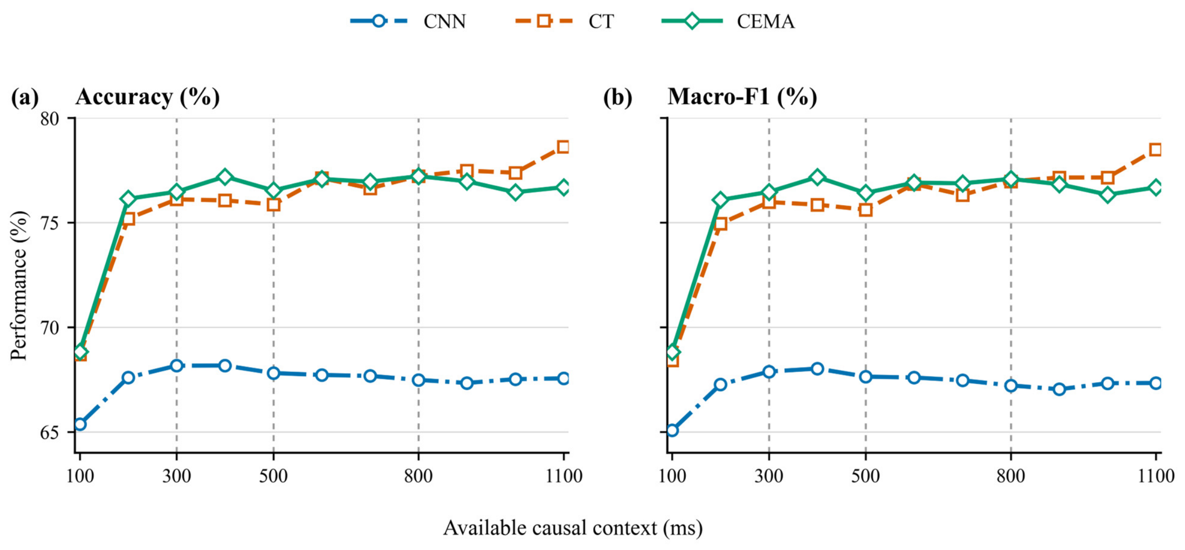
The complete-context analysis used $W=100$ ms current windows and m$=$0–10 (100–1100 ms), one fit per architecture × fold × context, training seed 0, and no enforced deterministic algorithms. Selected numerical values from the curve are provided in Supplementary Table S1. These descriptive results do not estimate training-seed variability and are separate from the five-seed primary-anchor analysis in Section 3.1.2.

Across the seed-0 curve, CNN changed little beyond 300 ms, CEMA improved rapidly at short-to-intermediate contexts and then remained relatively stable, and CT continued to improve at longer contexts. Accuracy and Macro-F1 followed closely aligned trajectories across the complete context range, as shown in Figure 1.

3.1.2. Training-Seed Robustness at the Primary Context Anchors

All 225 planned deterministic fits were completed. Across model–anchor combinations, the seed SD of five-fold mean accuracy ranged from 0.164 to 0.632 percentage points, and the corresponding Macro-F1 SD ranged from 0.165 to 0.692 points. Full seed means, SDs, and ranges are provided in Supplementary Table S2a.

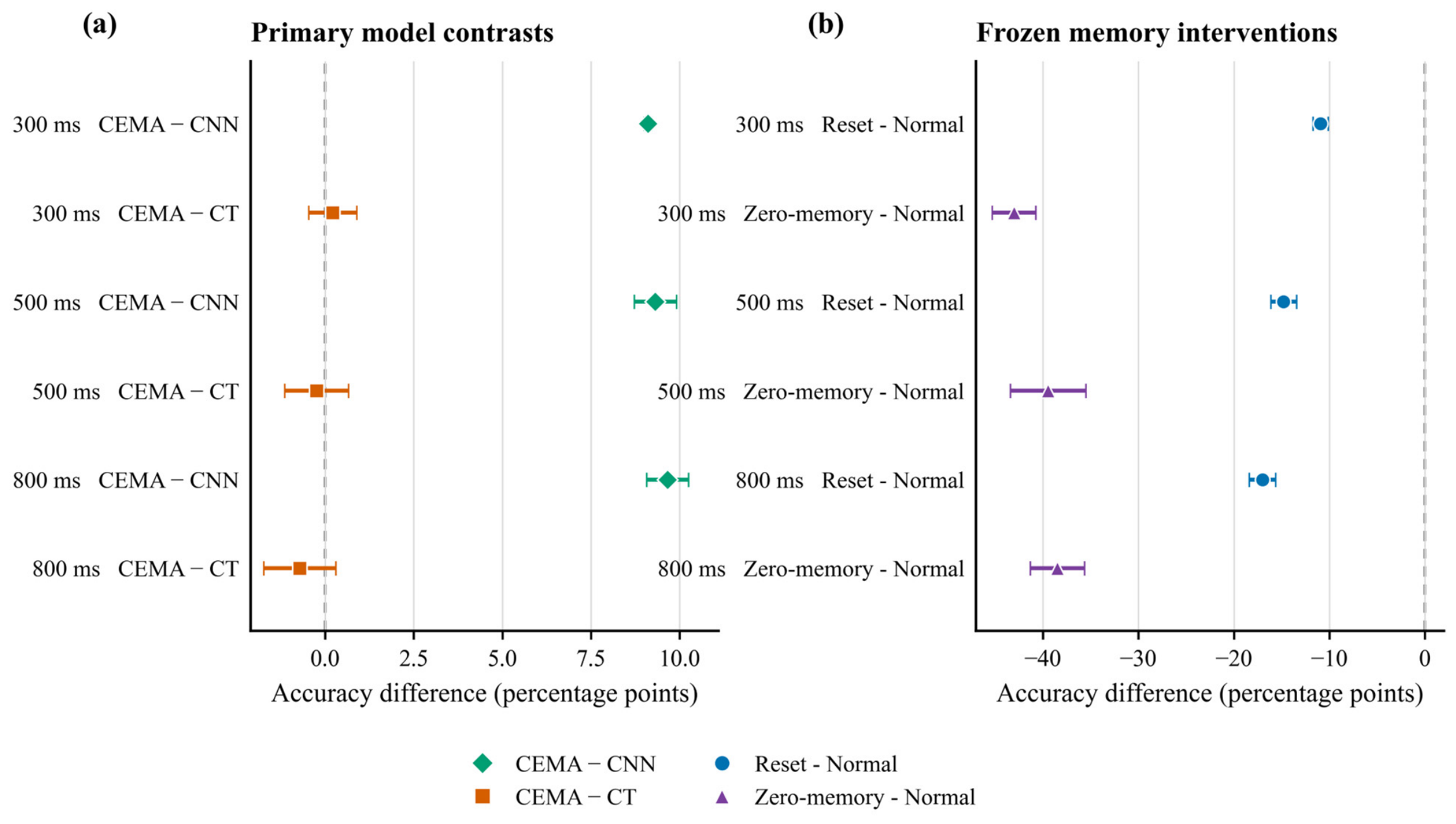
After seeds were averaged within each held-out fold, CEMA accuracy exceeded CNN accuracy by +9.105, +9.313, and +9.657 percentage points at 300, 500, and 800 ms, respectively; the respective 95% CIs were [+8.994, +9.215], [+8.721, +9.905], and [+9.067, +10.246], and all Holm-adjusted paired-t p values were < 0.001 (

Table 2. Paired accuracy differences at the primary context anchors, with five training seeds averaged within each fold.

Context (ms)	Contrast	Mean Difference (pp)	95% CI	Cohen’s dz	Holm-Adjusted p Value
300	CEMA−CNN	+9.105	[+8.994, +9.215]	102.45	p < 0.001
300	CEMA−CT	+0.209	[−0.467, +0.885]	0.38	p = 0.877
500	CEMA−CNN	+9.313	[+8.721, +9.905]	19.53	p < 0.001
500	CEMA−CT	−0.240	[−1.141, +0.661]	−0.33	p = 0.877
800	CEMA−CNN	+9.657	[+9.067, +10.246]	20.34	p < 0.001
800	CEMA−CT	−0.715	[−1.730, +0.300]	−0.87	p = 0.367

Note. Values are paired accuracy differences across five seed-averaged held-out folds. For each fold, the five training-seed differences were averaged before inference; the 25 seed × fold values were not treated as independent observations. Confidence intervals are two-sided 95% paired-t intervals; p values are two-sided paired-t results Holm-adjusted jointly across the six anchor contrasts. Very large $d_z$ values for CEMA−CNN reflect the small between-fold variability of the seed-averaged paired differences; interpretation emphasizes the mean differences and confidence intervals.

). The difference was positive for every training seed at every anchor (Supplementary Table S2b).

For CEMA−CT, the fold-first accuracy differences were +0.209 points at 300 ms (95% CI [−0.467, +0.885], Holm-adjusted p = 0.877), −0.240 points at 500 ms ([−1.141, +0.661], p = 0.877), and −0.715 points at 800 ms ([−1.730, +0.300], p = 0.367). The direction changed across seeds at every anchor: 3 positive/2 negative at 300 ms and 1 positive/4 negative at both 500 and 800 ms; individual seed contrasts are in Supplementary Table S2b.

Thus, the large CEMA−CNN accuracy gain was robust to training seed, whereas the much smaller CEMA−CT difference did not show a stable direction. The five-seed analysis does not support a consistent pointwise accuracy advantage of CEMA over CT at the primary anchors; because no equivalence margin was tested, it also does not establish equivalence.

3.2. CEMA History-Content Ablation

3.2.1. Trained History-Content Ablations

The seed-0 auxiliary analysis compared chronological history with an independently trained $m=0$ no-history checkpoint, deterministically window-shuffled history, and masked history. These controls change checkpoint parameters, optimization trajectories, or inputs and, therefore, do not isolate the EMA state with parameters fixed. Their descriptive means are retained in

Table 3. Single-seed trained history-content ablations at the primary context anchors.

$\mathit{m}$	Condition	Accuracy	Macro-F1
2	Chronological history	76.47	76.47
2	No history	68.84	68.83
2	Window-shuffled history	76.37	76.26
2	Masked history	69.08	69.07
4	Chronological history	76.54	76.42
4	No history	68.84	68.83
4	Window-shuffled history	76.26	76.17
4	Masked history	69.24	69.21
7	Chronological history	77.22	77.09
7	No history	68.84	68.83
7	Window-shuffled history	75.29	75.21
7	Masked history	69.43	69.47

Note. Values are seed-0 five-fold mean accuracy and Macro-F1 (%). Conditions may differ in trained parameters or optimization trajectory and should not be interpreted as frozen-checkpoint interventions.

; detailed paired results are provided in Supplementary Note S1, and a complementary frozen-checkpoint diagnostic is reported in Section 3.2.2.

Chronological history exceeded the independently trained no-history and masked-history controls at all three anchors (all six Holm-adjusted paired-t p ≤ 0.0021), although exact tests had a coarse resolution with five folds. Window shuffling produced its largest mean reduction at 800 ms, but the Holm-adjusted p value was 0.073. These results are supportive single-seed evidence rather than isolated frozen-parameter effects (Supplementary Note S1).

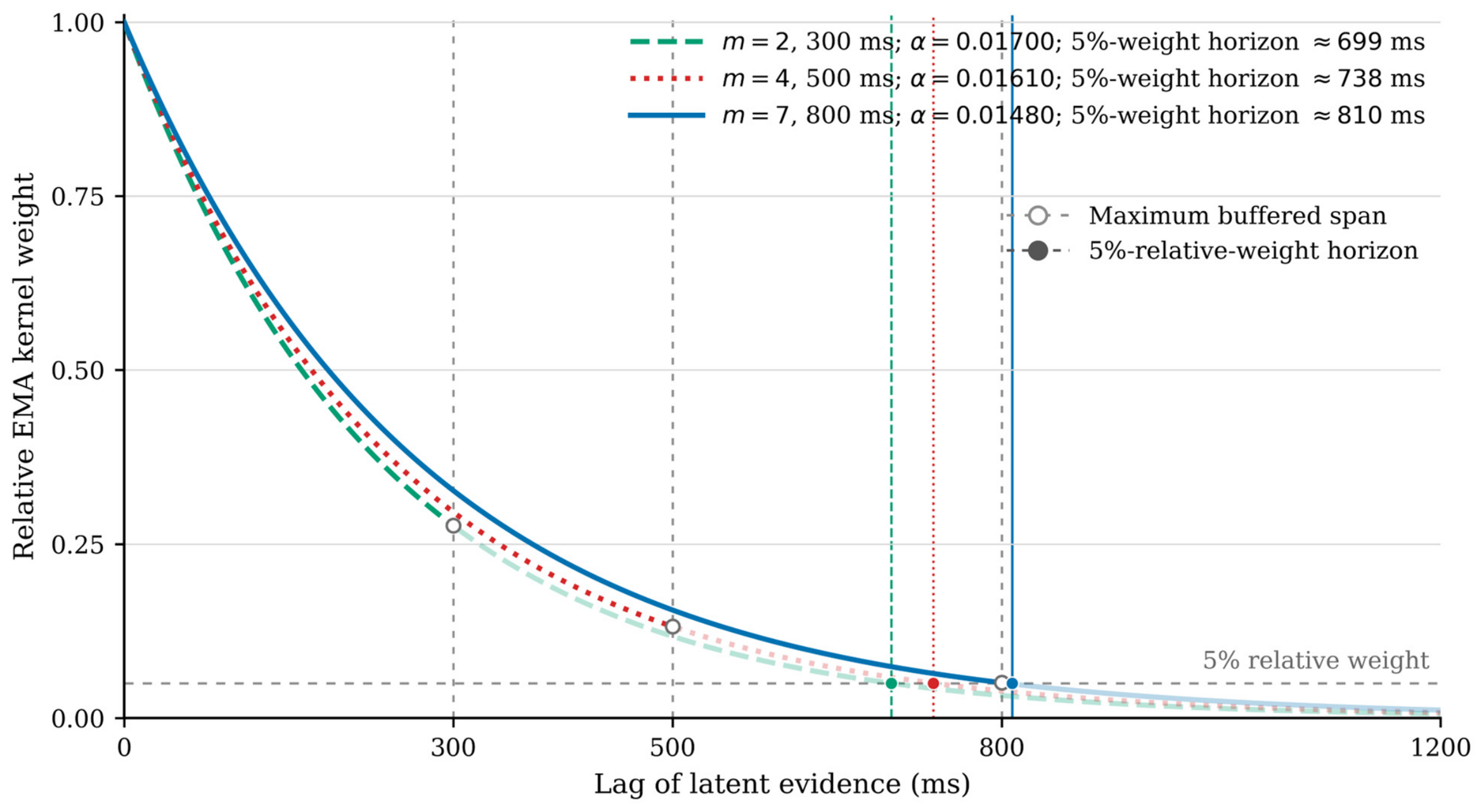
The three seed-0 CEMA context models each used a single learned decay scale, with continuous five-relative-weight horizons of approximately 699, 738, and 810 ms at 300, 500, and 800 ms, respectively. Because the EMA state was reset at each buffered-sequence start, usable memory was truncated by the corresponding input buffer. The learned lag-weight profiles and their truncation by the available input buffers are shown in Figure 2.

The trained history controls, therefore, motivate but do not replace the frozen-checkpoint diagnostic below.

3.2.2. Frozen-Checkpoint Diagnostic Memory Ablation Results

All 75 deterministic five-seed CEMA checkpoints completed the three frozen inference conditions, and normal reproduced the source outputs. Relative to normal, reset-at-current-window reduced accuracy by 10.928–17.009 points across anchors, whereas zero-memory reduced it by 38.485–43.028 points; corresponding Macro-F1 effects and fold-first confidence intervals are reported in

Table 4. Fold-first five-seed paired effects of frozen-checkpoint memory interventions relative to normal chronological memory.

Context (ms)	Contrast	Δ Accuracy (pp) [95% CI]	Holm-Adjusted p Value	Δ Macro-F1 (pp) [95% CI]	Holm-Adjusted p Value
300	Reset−Normal	−10.928 [−11.722, −10.134]	p < 0.001	−11.218 [−12.142, −10.293]	p < 0.001
300	Zero-memory−Normal	−43.028 [−45.319, −40.738]	p < 0.001	−51.990 [−54.386, −49.593]	p < 0.001
500	Reset−Normal	−14.791 [−16.143, −13.439]	p < 0.001	−15.925 [−17.775, −14.074]	p < 0.001
500	Zero-memory−Normal	−39.451 [−43.407, −35.495]	p < 0.001	−48.708 [−53.317, −44.099]	p < 0.001
800	Reset−Normal	−17.009 [−18.387, −15.631]	p < 0.001	−18.063 [−19.356, −16.770]	p < 0.001
800	Zero-memory−Normal	−38.485 [−41.311, −35.659]	p < 0.001	−47.405 [−50.772, −44.038]	p < 0.001

Note. Differences are intervention minus normal and are based on five seed-averaged held-out folds. The five training-seed differences were averaged within-fold before inference; 25 seed × fold values were not treated as independent. Confidence intervals are two-sided 95% paired-t intervals. p values are Holm-adjusted separately across six context-by-intervention contrasts for accuracy and Macro-F1. These frozen interventions can introduce distribution shift and are diagnostic rather than new training conditions.

. All twelve metric-specific Holm-adjusted paired-t p values were <0.001.

These paired frozen-checkpoint drops directly show that predictions depend strongly on the learned EMA-memory pathway when all remaining parameters are fixed. They do not define new training conditions or a fully history-free model: Reset retains the full input and finite-receptive-field encoder history, and both interventions can induce distribution shift. Accordingly, the frozen diagnostic is interpreted separately from the independently trained no-history result in Section 3.2.1; no statistical comparison between those two evidence families was performed.

The fold-first five-seed CEMA–CNN accuracy effects were positive at all three contexts, whereas the smaller CEMA–CT differences had confidence intervals spanning zero. Both frozen-checkpoint interventions produced marked negative accuracy changes, with zero-memory producing larger reductions than reset-at-current-window. Together, the primary model contrasts and frozen-checkpoint intervention effects are summarized in Figure 3.

3.3. Boundary Behavior, Smoothing Controls, and Stream-Level Sensitivity Analysis

3.3.1. Window-Internal Boundary Behavior and Smoothing Controls

Pointwise accuracy and transition counts cannot alone characterize dense recognition: fewer changes may reflect either reduced fragmentation or delayed/missed true boundaries.

Table 5. Representative window-internal B50 accuracy–boundary trade-offs at 300 and 800 ms.

Model Context	Accuracy (%)	B50 Recall (%)	Missed Transitions (%)	Absolute Delay (ms)	False Transitions (per 1000)	Stable Flips (per 1000)
CT raw, $(m=2)$	76.1	56.5	43.5	15.3	7.04	7.26
CEMA raw, $(m=2)$	76.5	43.6	56.4	16.7	7.03	7.22
CNN causal median, $(m=2)$	76.6	28.9	71.1	20.8	2.35	2.45
CT raw, $(m=7)$	77.2	59.1	40.9	15.0	6.29	6.51
CEMA raw, $(m=7)$	77.2	44.5	55.5	14.8	8.34	8.54

Note. B50 denotes one-to-one boundary matching within ±50 ms and serves as the primary localization-sensitive endpoint.

, therefore, summarizes representative window-internal B50 recall, missed rate, absolute delay, false transitions, and stable flips for raw CT/CEMA and a validation-selected causal-median CNN control.

At 300 ms, CT and CEMA achieved similar accuracy and nearly identical false-transition and stable-flip rates, but CEMA showed lower B50 recall (43.6% versus 56.5%), more missed transitions, and longer absolute delay. At 800 ms, their rounded accuracy was again identical, whereas CT retained higher recall and fewer missed transitions, and CEMA produced more false transitions and stable flips. The validation-selected causal-median CNN control reduced false transitions and stable flips but at the cost of lower recall and longer delay, which illustrates a smoothing–boundary trade-off; this control represents post hoc output smoothing rather than the proposed EMA latent memory mechanism. Although the window-internal definition excluded window-start transitions uniformly and left pointwise metrics unchanged, event-level bias could not be assumed to be negligible; Section 3.3.2, therefore, restores eligible within-recording joins. Overall, the window-internal results indicate an accuracy–boundary trade-off: neither fewer predicted transitions nor high pointwise accuracy alone demonstrates better temporal behavior.

3.3.2. Stream-Level Boundary Behavior

We evaluated all 225 deterministic five-seed checkpoints after stitching exactly contiguous current-window predictions within each subject and original recording. The five held-out folds contained 720 recordings and 601,048 eligible joins; none crossed a recording or subject boundary.

Table 6. Stream-level B50/B100 precision, recall, and F1 at the primary context anchors.

Context (ms)	Model	B50 Precision	B50 Recall	B50 F1	B100 Precision	B100 Recall	B100 F1
300	CNN	0.007 ± 0.001	0.982 ± 0.005	0.013 ± 0.001	0.007 ± 0.001	0.996 ± 0.002	0.014 ± 0.001
300	CT	0.024 ± 0.004	0.722 ± 0.034	0.046 ± 0.007	0.030 ± 0.004	0.893 ± 0.020	0.057 ± 0.008
300	CEMA	0.022 ± 0.003	0.601 ± 0.022	0.042 ± 0.005	0.030 ± 0.004	0.844 ± 0.015	0.059 ± 0.008
500	CNN	0.007 ± 0.001	0.981 ± 0.004	0.013 ± 0.001	0.007 ± 0.001	0.996 ± 0.002	0.014 ± 0.001
500	CT	0.025 ± 0.004	0.716 ± 0.033	0.049 ± 0.008	0.031 ± 0.005	0.880 ± 0.020	0.060 ± 0.010
500	CEMA	0.019 ± 0.003	0.526 ± 0.037	0.036 ± 0.005	0.027 ± 0.004	0.751 ± 0.028	0.052 ± 0.008
800	CNN	0.007 ± 0.001	0.982 ± 0.005	0.014 ± 0.001	0.007 ± 0.001	0.996 ± 0.002	0.014 ± 0.001
800	CT	0.027 ± 0.005	0.731 ± 0.037	0.052 ± 0.009	0.033 ± 0.005	0.889 ± 0.020	0.063 ± 0.009
800	CEMA	0.018 ± 0.003	0.519 ± 0.043	0.034 ± 0.005	0.025 ± 0.004	0.724 ± 0.033	0.048 ± 0.008

Note. Values are mean ± SD across five held-out subject folds after the five training seeds were averaged within each fold. B50 and B100 use greedy closest one-to-one matching within ±50 and ±100 ms, respectively. Precision, recall, and F1 are proportions.

reports B50/B100 precision, recall, and F1, while signed/absolute delay, missed rate, and false transitions are provided in Supplementary Table S3.

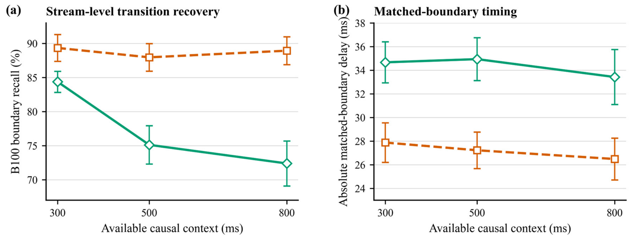
At B100, CNN achieved a recall of 0.996 at every anchor but a precision of 0.007 and approximately 40 false transitions per 1000 samples, which indicates extensive fragmentation. At 300, 500, and 800 ms, CT had higher B100 recall than CEMA, and the CEMA recall deficit widened with context (paired differences: −4.97, −12.84, and −16.54 percentage points, respectively; lower in all five folds). CEMA also had consistently longer absolute matched-boundary delay, but the mean increments were +6.79, +7.71, and +6.94 ms, respectively, all below 8 ms (<0.08 of the 100 ms current window). The main separation was, therefore, in recovered transitions rather than an extreme timing offset among matched events; false-transition differences changed with context (Supplementary Table S3), and no general CEMA boundary advantage was supported. The contrast between transition recall and matched-boundary timing is shown in Figure 4.

Restoring valid within-recording joins generally increased CT/CEMA B50 and B100 F1 and reduced missed-transition rates while also increasing matched delays and false transitions. Detailed stream-minus-window differences are provided in Supplementary Note S2; seam handling, therefore, changes event recovery and matching geometry jointly.

This sensitivity analysis uses chronologically stitched predictions from saved full-buffer checkpoints. It evaluates boundary accounting across consecutive windows, not incremental execution, embedded-system timing, online operation, or deployment validation.

3.4. Computational Efficiency, Storage, and Inference Time

Efficiency was evaluated using batch-size-1 full-buffer host-wall time, analytic forward MACs, parameter count, persistent buffers, and checkpoint size. Across all anchors, CEMA required fewer MACs and less host-wall time than CT, while CNN remained the lightest and fastest implementation.

Table 7. Full-buffer inference cost and model size at 300, 500, and 800 ms.

Model	Host-Wall Time (ms), 300/500/800	Forward MACs (M), 300/500/800	Learnable Parameters	Persistent Buffer (KiB)	Checkpoint (KiB)
CNN	0.311/0.308/0.307	0.623/1.038/1.661	6407	0.00	29.49
CT	1.206/1.193/1.188	1.444/2.806/5.450	12,967	3125.00	3189.05
CEMA	0.521/0.515/0.515	0.751/1.352/2.403	6968	0.00	33.11

Note. Context-specific values are ordered 300/500/800 ms. Host-wall times are five-checkpoint means at batch size 1. MACs include the causal encoder, temporal path, and classifier. CT’s positional encoding is a nonlearnable persistent buffer and is excluded from its learnable parameter count.

summarizes the measured context-specific costs and model sizes.

At the 300 ms anchor, CEMA required 0.521 ms per full-buffer forward, compared with 1.206 ms for CT and 0.311 ms for CNN. Under this benchmark, CT, therefore, required 2.31 times the CEMA host-wall time. CEMA also used 0.751 M forward MACs, compared with 1.444 M for CT, corresponding to a 48.0% reduction. These results show that CEMA was substantially lighter than CT.

As context length increased, analytic forward MACs rose for both temporal models, with a steeper increase for CT than for CEMA. CEMA required fewer MACs than CT at all three anchors. For each model individually, however, measured host-wall time changed only slightly from 300 to 800 ms. Thus, under the tested GPU and implementation, the substantial increase in analytic MACs was not accompanied by a comparable increase in measured inference time. This observation is specific to the reported hardware and code path. The benchmark included the full-buffer dense forward pass, final-current-window logit selection, and argmax but excluded pre-processing, history-buffer construction, host-to-device transfer, file I/O, scheduling, and external control-loop latency.

CEMA added 561 learnable parameters relative to CNN and remained substantially smaller than CT; its checkpoint footprint was close to that of CNN, whereas CT’s was dominated by the released implementation’s persistent positional-encoding buffer (Table 7).

CT contained approximately 1.86 times as many learnable parameters as CEMA. The difference in serialized checkpoint size was much larger, mainly because the released CT implementation stored a 3125.00 KiB nonlearnable positional-encoding buffer covering 50,000 latent positions. This buffer increased checkpoint storage but was not included in the learnable parameter count. CEMA also has a fixed-state incremental formulation. At each latent step, the EMA update requires $O\left(d\right)$ state memory and $O\left(d\right)$ recurrent computation, while the fusion projection requires $O\left(d^2\right)$ computation. However, the reported benchmark evaluated the released full-buffer implementation, which recomputed the complete buffered sequence for every input example. It did not test an incremental encoder, persistent state across successive updates, or a complete streaming pipeline. The theoretical incremental formulation, therefore, should not be interpreted as a measured incremental-execution advantage or reduction in end-to-end latency.

Overall, CEMA occupied an intermediate efficiency position between CNN and CT. Under the reported full-buffer implementation, CEMA required fewer analytic MACs, fewer learnable parameters, less checkpoint storage, and lower host-wall time than CT, whereas CNN remained the lightest and fastest model. These comparisons apply only to the reported hardware, software, and execution path. The potential advantages of incremental CEMA execution remain to be experimentally validated.

3.5. Classwise Recognition Performance

Five-seed classwise F1 at 300 ms was examined descriptively after averaging seeds within each held-out fold. CEMA exceeded CNN for all seven class means and for every seed-specific class contrast, which indicates that the aggregate gain was not driven by one class; complete fold-first values are in Supplementary Table S4.

The largest CEMA–CNN mean gains were for Supination (+12.3 points), Pronation (+11.9), and Hand Open (+11.0). CEMA–CT class differences ranged from −0.78 to +1.43 points and varied in direction across seeds for most classes; no class-specific inferential or equivalence claim is made.

These descriptive classwise results support the broad CEMA–CNN gain but do not establish improved boundary behavior, which is evaluated separately in Section 3.3.

4. Discussion

4.1. Principal Findings and Contributions

The five-seed analyses support a stable CEMA pointwise gain over CNN at the three primary anchors, whereas the small CEMA–CT differences changed direction across seeds and established neither superiority nor equivalence (Table 2). Frozen interventions showed strong dependence on the EMA-memory pathway but with distribution-shift and residual-encoder-history caveats (Table 4). Stream-level stitching showed no general CEMA boundary advantage, while CEMA retained a lower measured model cost than CT. CEMA is, therefore, a lightweight temporal-memory alternative, not a general replacement for attention.

4.2. Interpretation of the Single-Scale EMA Mechanism

CEMA uses one shared decay scale, so historical weighting depends on temporal distance rather than content. With parameters frozen, reset-at-current-window reduced accuracy by 10.9–17.0 points and zero-memory by 38.5–43.0 points across anchors. These drops demonstrate pathway dependence, not a pure causal history effect: reset retains encoder history, zero-memory is a stronger intervention, and both can induce distribution shift. The independently trained no-history and shuffled/masked controls remain separate seed-0 auxiliary evidence.

The seed-0 context curve and ordering ablation suggested possible long-context limits, but the five-seed 800 ms CEMA–CT confidence interval included zero, and the shuffled-history effect was not significant after Holm correction. These patterns motivate, but do not prove the need for, multi-scale or content-adaptive memory.

4.3. Accuracy–Boundary Trade-Off and Smoothing Controls

High pointwise accuracy did not imply accurate transition localization. Relative to CT, CEMA’s mean B100 recall deficit was 4.97–16.54 percentage points, and its mean absolute-delay increment was 6.79–7.71 ms (<0.08 of the 100 ms current window). These transition-local costs limit transition-sensitive applications but do not negate CEMA’s stable pointwise accuracy gain over CNN. No general CEMA boundary or stability advantage is claimed.

Restoring within-recording joins changed event recovery, delay, and false transitions jointly. The seed-0 causal-median control likewise reduced isolated flips at the cost of recall and delay. Both analyses use saved full-buffer predictions and do not validate incremental or real-time execution.

4.4. Efficiency and Implementation Implications

The CEMA implementation used fewer analytic MACs, fewer learnable parameters, a smaller serialized checkpoint, and a lower measured host-wall time than the matched CT implementation. These quantities describe different aspects of the evaluated implementation: MACs estimate model-side arithmetic, parameter count describes trainable capacity, checkpoint size includes serialized buffers, and host-wall time depends on hardware, software, and the measured execution path. CNN remained the lightest and fastest evaluated model. CT’s larger checkpoint footprint was driven mainly by a nonlearnable positional-encoding buffer in this implementation and should not be generalized to all Transformer designs.

CEMA, therefore, occupied a favorable measured efficiency position between CNN and the matched CT implementation. Its mathematical recurrence permits a fixed-state update, but every reported timing measurement recomputed the full input buffer at batch size 1. No incremental encoder, persistent-state runtime, acquisition or transmission path, scheduler, controller, or embedded device was evaluated. The findings support model-level full-buffer efficiency on the tested host only; they do not validate online deployment, end-to-end latency, incremental-execution advantages, or embedded-system performance.

4.5. Classwise Findings, Limitations, and Future Directions

The five-seed classwise results showed CEMA–CNN gains across all seven classes, whereas the small CEMA–CT class differences were mostly direction dependent; no class-specific inference or equivalence claim was made (Supplementary Table S4).

The experimental validation was limited to a single publicly available dataset comprising 30 participants. Although the subject-independent design evaluates generalization to held-out participants within this dataset, it does not establish that the findings generalize to other datasets, acquisition protocols, electrode configurations, participant populations, or motion tasks. Validation on additional independent sEMG datasets would, therefore, strengthen the generality of the conclusions. Other limitations include five held-out folds, retrospective selection of the primary context anchors, one shared EMA decay scale, distribution shift in the frozen interventions, and stitched rather than incremental boundary evaluation. Fixed single-scale EMA smoothing may contribute to transition inertia, but this mechanism was not isolated, and CEMA was not evaluated as a dedicated onset detector. The complete context curve, trained history controls, smoothing analysis, and supplementary W = 10 ms pilot remain seed-0 descriptive or auxiliary evidence.

Future work should prioritize external validation on additional independent datasets and should further examine prospectively defined anchors, repeated-seed auxiliary analyses, multi-scale or content-adaptive memory, boundary-aware objectives, persistent-state execution, embedded hardware, and end-to-end control loops.

5. Conclusions

This study evaluated CEMA for dense sEMG motion recognition within a matched strictly causal encoder–decoder framework. At the 300, 500, and 800 ms primary context anchors used for the multi-seed analysis, the fold-first five-seed results showed stable CEMA accuracy gains over CNN, whereas the small CEMA–CT differences changed direction and did not establish either a stable CEMA advantage or equivalence. The frozen-checkpoint diagnostic showed a strong dependence on the learned EMA-memory pathway with all parameters fixed, while its distribution-shift and residual encoder-history limitations preclude interpreting the drops as a pure causal history effect. The five-seed classwise results further showed that the CEMA–CNN gain extended across all seven classes.

Boundary evaluation showed that CT had a higher B100 recall by 4.97–16.54 percentage points, while CEMA’s mean absolute delay was 6.79–7.71 ms longer; false-transition differences were context-dependent. CEMA required fewer parameters, analytic MACs, checkpoint storage, and measured host-wall time than the matched CT implementation. These findings indicate a favorable trade-off between average accuracy and efficiency for CEMA, whereas CT showed greater transition responsiveness under the evaluated boundary metrics. The reported host-wall timing measurements were obtained only for batch-size-1 full-buffer inference, in which the complete buffered sequence was recomputed for each input. Although the EMA recurrence permits a fixed-state formulation, no persistent-state incremental streaming implementation was benchmarked; its streaming latency and efficiency, therefore, remain to be experimentally validated. Accordingly, no claim is made regarding incremental, embedded, or end-to-end deployment performance. One shared decay scale, one dataset, five held-out folds, and seed-0 auxiliary analyses further limit generalization.

Overall, CEMA offers a favorable average accuracy–efficiency trade-off: it provides a seed-robust pointwise gain over CNN and a lower measured cost than CT, while CT remains more responsive at transitions. It is a lightweight strictly causal sequence-level alternative, not a dedicated transition detector or a general replacement for attention. Future work should experimentally validate persistent-state incremental streaming and end-to-end deployment, while also examining boundary-aware or multi-scale memory.