A Novel TabPFN-Based Framework for Landslide Susceptibility Assessment: Multi-Model Comparison in Qingchuan County, Sichuan, China

Abstract

Landslides are among the most common and destructive geological hazards in complex mountainous regions. Developing accurate and interpretable susceptibility assessment models is important for regional geological hazard prevention and spatial safety management. To address the limitations of traditional machine learning models in processing tabular geoscience data with limited samples and complex nonlinear relationships, this study took Qingchuan County, Sichuan Province, as the study area and introduced the Tabular Prior-data Fitted Network (TabPFN) for landslide susceptibility assessment. Its performance was systematically compared with four commonly used models: Logistic Regression (LR), Support Vector Machine (SVM), Random Forest (RF), and Extreme Gradient Boosting (XGBoost). An evaluation system was built using 12 conditioning factors, including elevation, lithology, and distance to roads (DTR). The SHapley Additive exPlanations (SHAP) method was further used to identify the contributions and effects of the main controlling factors. The results showed that TabPFN achieved the highest observed predictive performance among the evaluated models, with an AUC of 0.7834, showing higher observed performance than traditional models such as LR, SVM, RF, and XGBoost, indicating its strong ability to capture nonlinear relationships and good applicability under limited sample conditions. SHAP analysis further indicated that elevation, lithology, and distance to roads were the main controlling factors influencing the model predictions. This study demonstrates the applicability of TabPFN for landslide susceptibility assessment in complex mountainous regions and provides a new methodological reference for intelligent geological hazard prediction and refined regional risk management under limited data conditions.

1. Introduction

Landslides are characterized by sudden occurrence, wide spatial distribution, and severe destructive impacts. Their formation is controlled by the combined effects of multiple factors, including topography, geomorphology, hydrology, geological conditions, and human activities. Landslides pose serious threats to the lives and property of residents in mountainous areas, as well as to engineering construction and the sustainable development of ecological environments. Against the background of intensifying climate change and increasing human engineering activities, the frequency and risk of landslide disasters continue to rise. Therefore, scientific and accurate landslide susceptibility assessment is an essential prerequisite for regional geological disaster prevention and control, risk management, and land-use planning [1,2].

Landslide susceptibility refers to the relative likelihood or spatial probability of landslide occurrence within a given area [3]. At present, landslide susceptibility assessment methods have gradually evolved from traditional empirical and statistical approaches to a technical framework dominated by machine learning. Traditional empirical models, such as the Analytic Hierarchy Process (AHP) [4] and Fuzzy Logic (FL) [5], are highly subjective, depend heavily on expert experience, and are not well suited to describing complex nonlinear relationships. Statistical models, such as the Certainty Factor (CF) model [6], Frequency Ratio (FR) model [7], and Information Value Model (IVM) [8], are often based on the assumption of linear relationships between conditioning factors and landslide occurrence. These models have difficulty capturing the complex, nonlinear, and coupled interactions among multiple factors, such as topography, geology, hydrology, and human activities, which limits their predictive accuracy. Machine learning models, including Logistic Regression (LR) [9,10], Support Vector Machine (SVM) [11,12], Random Forest (RF) [13,14], and Extreme Gradient Boosting (XGBoost) [15,16], are widely used in landslide susceptibility assessment because of their strong nonlinear fitting capability and high predictive performance. These models achieve favorable results in various regional applications. However, traditional machine learning models still face several limitations in practical applications. Some models require extensive hyperparameter tuning and high computational costs. Under small-sample conditions, they are prone to overfitting or insufficient generalization. In addition, their learning efficiency and prediction stability vary considerably when handling complex environmental factors.

In recent years, Tabular Prior-Data Fitted Network (TabPFN) [17,18], a newly developed model for tabular data, has shown promising performance in small-sample classification tasks and has gradually been introduced into geohazard susceptibility assessment. Notably, Zhou et al. (2025) [19] applied TabPFN to landslide hazard assessment in Renhe District, Panzhihua City, Sichuan Province, and compared its performance with RF and XGBoost. Their results showed that RF outperformed TabPFN, with AUC values of 0.9471 and 0.9243, respectively, and they further pointed out the potential risk of overfitting when using TabPFN. Therefore, TabPFN should not be regarded as an entirely unexplored method in landslide hazard or susceptibility assessment. Instead, further validation is needed to examine its robustness and applicability across different geomorphological settings, sample sizes, conditioning-factor systems, and triggering environments. Compared with conventional machine learning models, TabPFN has potential advantages in prediction efficiency and stability. However, its application to landslide susceptibility assessment in tectonically active and topographically complex mountainous areas, such as Qingchuan County in the northern Longmen Mountains [20,21], remains limited. Unlike the Renhe District case investigated by Zhou et al. (2025) [19], Qingchuan County is located in the Longmen Shan earthquake-affected region and was strongly influenced by the 2008 Wenchuan earthquake, providing a distinct geomorphological and seismic context for further evaluating TabPFN. In addition, existing studies still lack systematic comparisons between TabPFN and commonly used machine learning models in such regions. Meanwhile, although machine learning models can improve the accuracy of landslide susceptibility prediction, their interpretability remains a concern. To better understand the influence of different conditioning factors on model outputs, the SHAP method can be used as an effective explanatory tool [22,23]. By introducing SHAP analysis, the relative importance and effects of key factors can be further identified, which helps improve the interpretability of landslide susceptibility assessment results.

Addressing issues in existing landslide susceptibility studies—such as insufficient model comparisons, weak explanatory power of influencing factors, and limited application of novel machine learning models—this study takes Qingchuan County as the research area. Twelve landslide-prone factors, including elevation, slope, lithology, and DTR, were selected to construct five models—LR, SVM, RF, XGBoost, and TabPFN—for landslide susceptibility assessment. Model performance was comprehensively evaluated using metrics such as accuracy, precision, recall, F1 score, ROC curves, and AUC, with a particular focus on the predictive accuracy, stability, and applicability of the TabPFN model. Based on these results, the SHAP method was employed to identify key controlling factors, explain the influence of each factor on landslide susceptibility, and reveal the spatial distribution patterns of landslide susceptibility in the study area. The research findings can serve as a reference for landslide disaster prevention and mitigation in Qingchuan County, as well as for the selection of susceptibility assessment models in similar mountainous regions.

2. Study Area and Dataset

2.1. Study Area

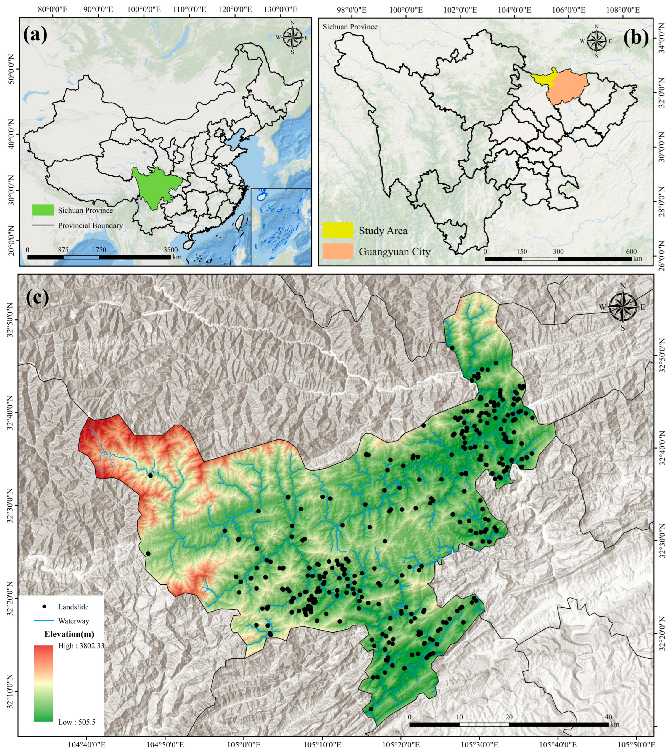
Qingchuan County, administered by Guangyuan City in Sichuan Province, is located at the junction of Sichuan, Shaanxi, and Gansu provinces, as shown in Figure 1. It lies on the northern margin of the Sichuan Basin, at the transition zone between the northern Longmen Mountains and the Min Mountains. The county extends from 32°12′ N to 32°56′ N in latitude and from 104°36′ E to 105°38′ E in longitude, covering an area of approximately 3216 km². Elevation ranges from 491 m to 3837 m. The terrain is dominated by medium-elevation mountains, accompanied by low mountains, hills, valleys, and small plains. Overall, the topography is higher in the northwest and lower in the southeast, forming a slightly crescent-shaped geomorphic pattern. The study area is situated within the Longmen Mountains seismic belt and is characterized by overlapping mountain ranges, deeply incised valleys, complex geological structures, and intense rock weathering. These conditions make the area highly susceptible to geological hazards such as landslides and debris flows.

2.2. Dataset

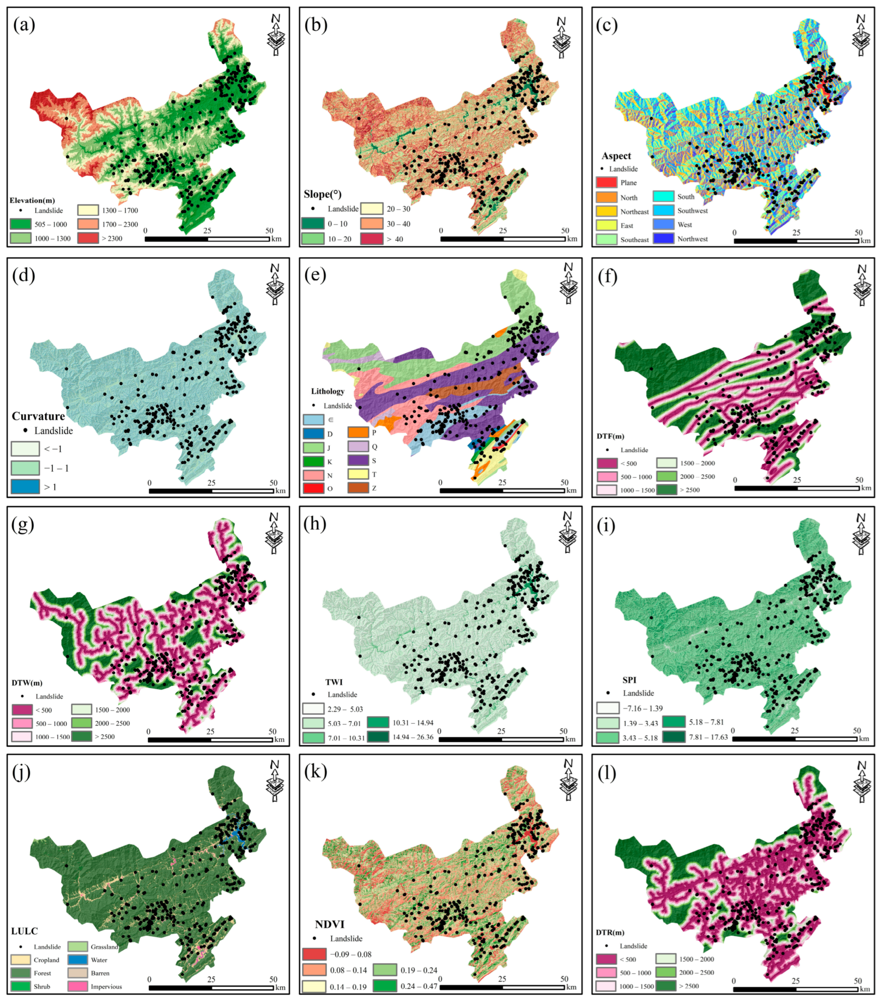
Topographic factors, including elevation, slope, aspect, curvature, Stream Power Index (SPI), and Topographic Wetness Index (TWI), were derived from the Copernicus 30 m Digital Elevation Model (DEM) using terrain analysis tools in ArcGIS 10.8. All raster datasets were resampled to a uniform spatial resolution of 30 m. Lithology and distance to faults (DTF) were obtained by vectorizing 1:1,000,000-scale geological maps. Fault lines were extracted, and Euclidean distance analysis was performed in ArcGIS to generate the DTF raster layer. Distance to watercourses (DTW) and distance to roads (DTR) were derived from OpenStreetMap (OSM) data, and the corresponding distance raster layers were generated using the Euclidean Distance tool in ArcGIS. Land use and land cover (LULC) data were obtained from the China Land Cover Dataset (CLCD) 30 m land-use product. The Normalized Difference Vegetation Index (NDVI) was derived from Landsat imagery and calculated using the standard NDVI formula on the Google Earth Engine (GEE) platform. Both LULC and NDVI datasets were processed into raster layers with a spatial resolution of 30 m. Landslide inventory data were obtained from the Data Center for Resources and Environmental Sciences. Projection transformation and clipping to the study area were conducted in ArcGIS, and the processed landslide points were used as sample data for model training and validation. The landslide inventory comprises 350 landslide points. To construct a balanced binary classification dataset, a 1 km buffer zone was generated around the existing landslide points, and an equal number of non-landslide points were randomly selected from areas outside the buffer zone. As a result, 700 samples were obtained in total. These samples were then divided into training and testing datasets at a ratio of 7:3, with 490 samples used for model training and 210 samples used for model validation. All datasets were projected into the WGS84 coordinate system to ensure spatial consistency. Detailed information on the datasets is provided in

Table 1. Detailed information on data.

Data Name	Data Source	Operating Platform	Resolution/Scale
Elevation, Slope, Aspect, Curvature, SPI, TWI	Copernicus DEM	ArcGIS	30 m
Lithology, DTF	geological map	ArcGIS	1:1,000,000
DTR, DTW	OSM	ArcGIS	Vector Data
LULC	CLCD	ArcGIS	30 m
NDVI	Landsat Imagery	GEE	30 m
Landslide Locations	Center for Resources and Environment	ArcGIS	Vector Data

. Because the landslide inventory was derived from a publicly available dataset, the original data mainly provide the spatial locations of landslides, while information on the occurrence time and failure type of each landslide is not systematically documented. Therefore, the temporal coverage of the landslide inventory could not be further specified, and the mapped landslides could not be reliably classified into specific failure types, such as rotational slides, translational slides, debris flows, or rockfalls. To avoid introducing additional uncertainty, this study used the inventory as a binary landslide/non-landslide dataset for regional-scale landslide susceptibility assessment.

3. Methodology

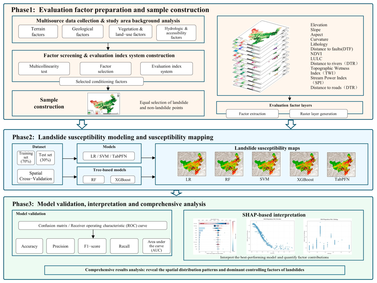
This study develops a landslide susceptibility assessment framework that integrates multi-source data-driven analysis, comparative model prediction, and mechanism-oriented interpretation. As illustrated in Figure 2, the framework is built upon multi-source geoscientific data from the study area, with key conditioning factors identified according to the characteristics of landslide development. Five models—LR, RF, SVM, XGBoost, and TabPFN—are employed for landslide susceptibility modeling and comparative evaluation, and the model showing the most promising predictive performance is further selected for interpretability analysis based on the model accuracy assessment. Compared with conventional approaches, this study applies TabPFN to landslide susceptibility assessment in complex mountainous areas. In addition, a comparative framework combining classical machine learning models with this emerging model is established, while SHAP is incorporated to extend the analysis from predictive performance to factor contribution identification and nonlinear mechanism interpretation. This framework therefore achieves a better balance among predictive accuracy, model applicability, and interpretability.

3.1. Landslide Susceptibility Prediction Models

3.1.1. Traditional Models

LR is a typical linear statistical model that uses the logistic function to describe the relationship between conditioning factors and the probability of landslide occurrence. Owing to its simple structure, clear parameter interpretation, and good interpretability, it is commonly used as a baseline model in landslide susceptibility assessment [24,25]. However, LR has limited capacity to capture complex nonlinear relationships among variables. In contrast, RF and XGBoost are both decision-tree-based ensemble learning models that can effectively model nonlinear relationships and complex interactions among multiple factors. Specifically, RF constructs multiple independent decision trees and derives the final prediction through voting or averaging, thereby showing strong resistance to overfitting and high stability [26,27]. XGBoost, based on the gradient boosting framework, builds decision trees sequentially and improves predictive performance by iteratively fitting the residuals of the previous model [28], thus generally providing higher accuracy and stronger feature representation capability [29,30]. SVM classifies samples by identifying the optimal classification hyperplane in a high-dimensional feature space [31]. With the use of kernel functions, it can effectively address nonlinear classification problems and is particularly suitable for landslide susceptibility prediction under small- to medium-sample conditions; however, its predictive performance is sensitive to the selection of kernel function type and parameter settings [32,33].

3.1.2. TabPFN

TabPFN was proposed by Hollmann et al. [34]. It is a Transformer-based generative foundation model specifically designed for tabular data. The core idea of TabPFN is to learn a general-purpose tabular data prediction algorithm from millions of synthetic datasets through in-context learning (ICL). By incorporating Bayesian prior inference, TabPFN can efficiently and accurately perform prediction tasks under limited-sample conditions. Therefore, it is particularly suitable for landslide susceptibility assessment in small-sample scenarios and can effectively reduce the risk of overfitting commonly encountered by traditional machine learning models when training data are scarce.

For a given training dataset and test samples, the predictive task of TabPFN can be expressed as follows:

$$p\left(y_{test} |{ X}_{test,}{X}_{train,}{y}_{train}\right)$$

(1)

where $X_{train}$ and $y_{train}$ denote the training features and corresponding labels, respectively, and $X_{test}$ represents the test features. The model directly predicts the posterior distribution of the labels for the test samples, thereby naturally incorporating uncertainty estimation. For classification tasks such as landslide susceptibility assessment, TabPFN outputs the probability distribution of each class.

$$\widehat{p}\left(y^{*}∣x^{*},D\right)=\int p\left(y^{*}∣x^{*},\theta \right)p\left(\theta ∣D\right)d\theta$$

(2)

where $D={\left\{\left(x_i,y_i\right)\right\}}_{i=1}^N$ represents the training dataset, and $\theta$ denotes the model parameters. TabPFN approximates this Bayesian integral using Transformer parameters, thus enabling end-to-end Bayesian inference.

Before being fed into the model, each cell in the tabular dataset is standardized using z-score normalization and then transformed into vector embeddings through linear encoding. The model employs a bidirectional attention mechanism to capture complex dependencies among samples and features. The attention mechanism is defined as:

$$\begin{array}{c}Attention\left(Q,K,V\right)=softmax\left({\displaystyle \frac{Q{K}^{\top }}{\sqrt{d_k}}}\right)V\end{array}$$

(3)

where $Q$, $K$, and $V$ denote the query, key, and value matrices, respectively, and $d_k$ is the dimensionality of the key vectors. Attention is calculated along both the sample and feature dimensions to capture complex relationships within tabular data.

During training, TabPFN maximizes the log-likelihood of hidden labels in the synthetic datasets. The loss function can be expressed as:

$$L=-\sum _{i=1}^{M}lg q_{\varphi }\left(y_i∣x_i,D_{-i}\right)$$

(4)

where $q_{\varphi }$ represents the predictive distribution of the model parameterized by Transformer weights $\varphi$, and $D_{-i}$ denotes the contextual samples excluding the $i$-th sample. Through this training strategy, TabPFN learns a prior over tabular prediction tasks and can rapidly infer the label distribution of unseen samples without extensive hyperparameter tuning.

3.2. Hyperparameter Optimization and Spatial Cross-Validation

To ensure fair and reproducible comparisons among the five models, namely LR, SVM, RF, XGBoost and TabPFN, hyperparameter optimization and performance evaluation were implemented within a unified spatial validation framework. A nested five-fold spatial block cross-validation approach was adopted to reduce the potential overestimation of predictive performance caused by spatial autocorrelation.

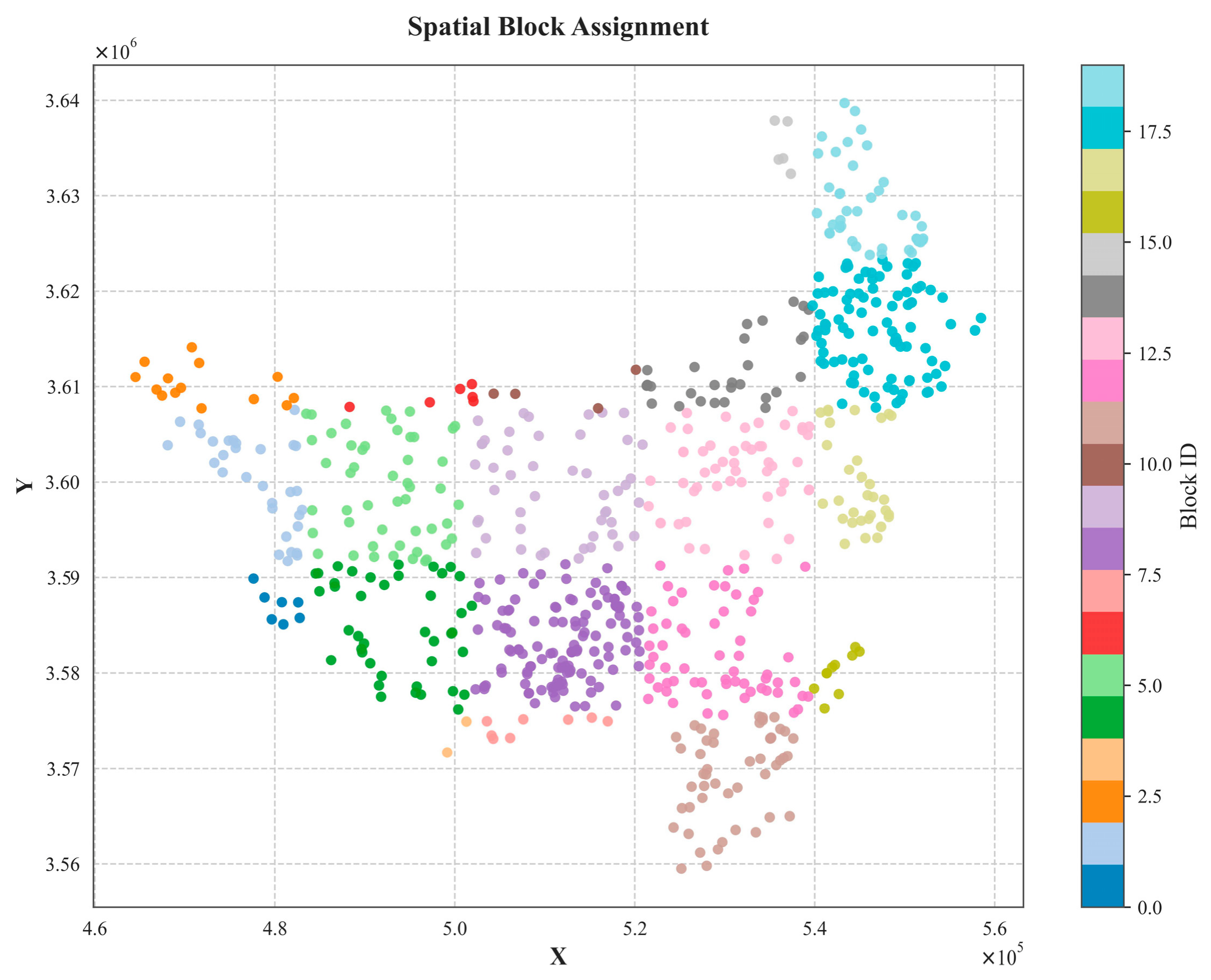
First, the samples in the study area were partitioned into multiple spatial blocks according to their spatial coordinates, and these blocks were subsequently assigned to five spatial folds for outer cross-validation (Figure 3). In each outer validation iteration, one spatial fold was used as the independent test set, whereas the remaining four folds were used as the training set. The outer test fold was completely excluded from data preprocessing, hyperparameter selection, and model fitting. Within each outer training set, grid search combined with inner cross-validation was used to optimize the hyperparameters of each model. The average AUC obtained from the inner validation was used as the criterion for selecting the optimal hyperparameter combination. After hyperparameter optimization, the model was refitted using the entire outer training set and then evaluated on the spatially independent outer test fold. This procedure was repeated until each spatial fold had been used once as the test set.

In each outer validation fold, AUC, accuracy, precision, recall and F1-score were calculated based on spatially independent test samples. Furthermore, out-of-fold predicted probabilities for all samples were aggregated, based on which the paired DeLong test was conducted to evaluate the statistical significance of AUC differences between models.

3.3. Multicollinearity Analysis

In landslide susceptibility assessment, correlations often exist among multiple conditioning factors. Strong multicollinearity among independent variables may weaken the stability of model parameter estimates and affect the identification of factor contributions, thereby reducing model predictive accuracy and interpretability. For this reason, the multicollinearity of the selected landslide-related variables was examined prior to model development [35]. In this study, the variance inflation factor (VIF) and tolerance (TOL) [36] were used as the main diagnostic indicators. These two metrics are reciprocal to each other, and their calculation formulas are expressed as follows:

$$VIF={\displaystyle \frac{1}{1-R^2}}$$

(5)

where $VIF$ denotes the variance inflation factor, and $R^2$ represents the coefficient of determination obtained by regressing the $i$-th independent variable against all the remaining independent variables.

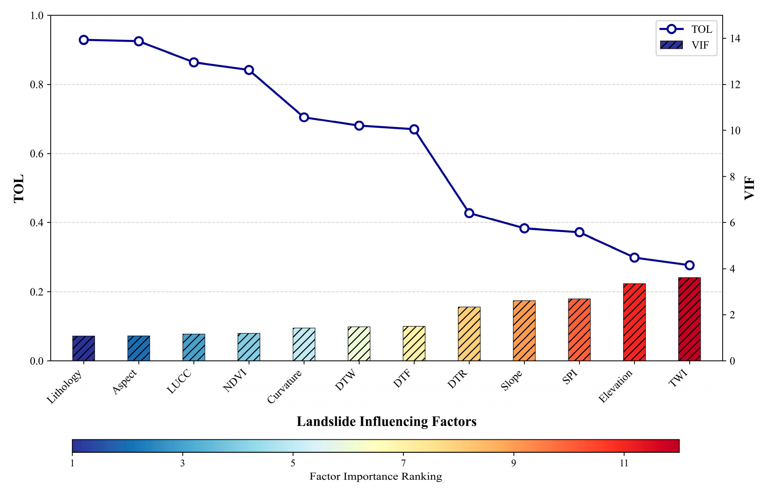
In general, strong multicollinearity among variables is considered to exist when TOL is less than 0.1, or VIF exceeds 10. A high VIF value indicates that a variable shares substantial overlapping information with other variables and should therefore be considered for exclusion or adjustment.

4. Results

4.1. Selection of Landslide Control Factors

The results of the multicollinearity analysis are shown in Figure 4. The TOL values of all 12 independent variables selected in this study (Figure 5) are greater than 0.1, and their VIF values are all less than 10. This indicates that no strong multicollinearity exists among the 12 independent variables. Thus, the variables can be regarded as relatively independent and satisfy the model’s requirement for variable independence.

4.2. Analysis of the Results Regarding Landslide Susceptibility

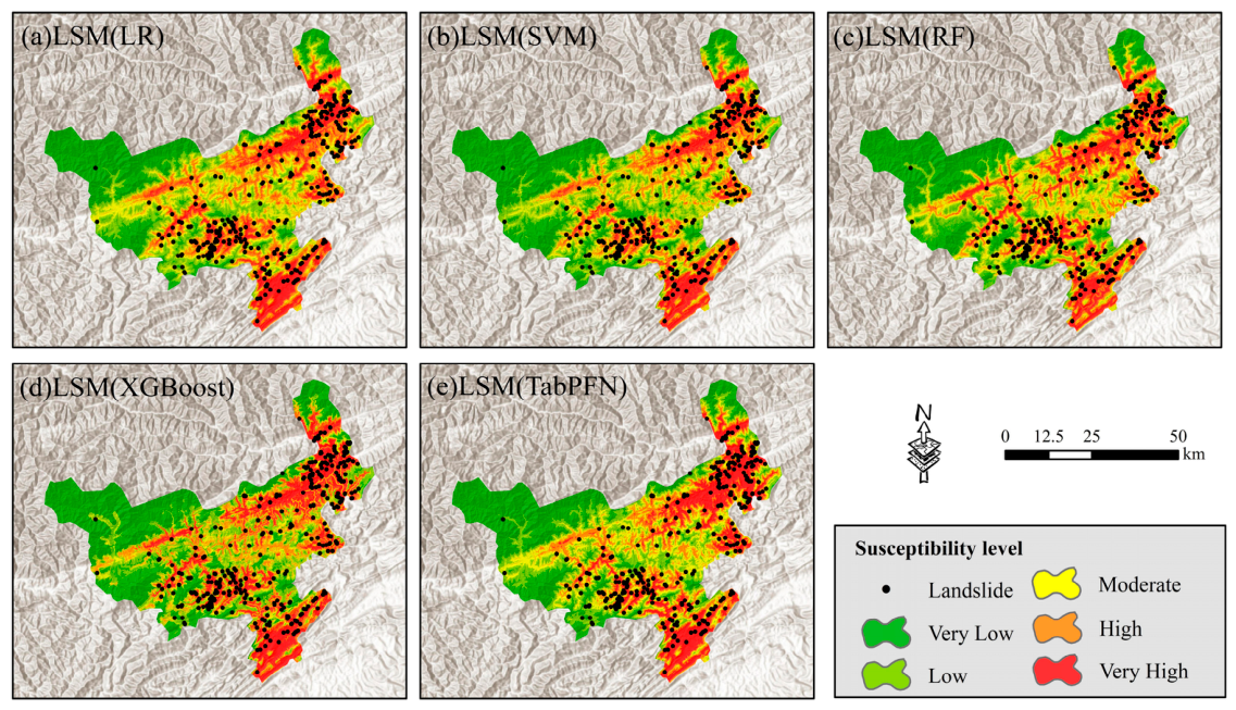
As shown by the landslide susceptibility zoning results of the five machine learning models (Figure 6), the very high- and high-susceptibility zones showed a clear strip-like distribution. The landslide susceptibility values shown in Figure 6 were classified into five levels, namely very low, low, moderate, high, and very high susceptibility, using the Natural Breaks (Jenks) classification method in ArcGIS. These zones extended along the main rivers in the central part of the county, including the Bailongjiang and Qingzhujiang river basins, as well as the deep gorges, covering most of the central-eastern and southern areas of the county. They constituted the main development areas of landslide hazards. The very low and low susceptibility zones were mainly concentrated in the high-altitude mountainous areas in the western and northern parts of the county. These areas were characterized by relatively gentle terrain and weak human engineering activities, resulting in a very low probability of landslide occurrence. The moderate-susceptibility zone acted as a transitional zone and was distributed in a ring-like and interlaced pattern between the high and low susceptibility zones, representing a potential area for landslide development. The spatial trends and extents of the very high and high susceptibility zones were generally consistent among the five models. In all models, landslide points were mainly distributed within the very high- and high-susceptibility zones, with only a small number located in the moderate susceptibility zone. Almost no landslide points were observed in the very low- and low-susceptibility zones. These results indicated a high degree of consistency among the zoning results of the five models and indirectly verified the reliability of the susceptibility assessment results.

4.3. Performance Evaluation of Landslide Susceptibility Models

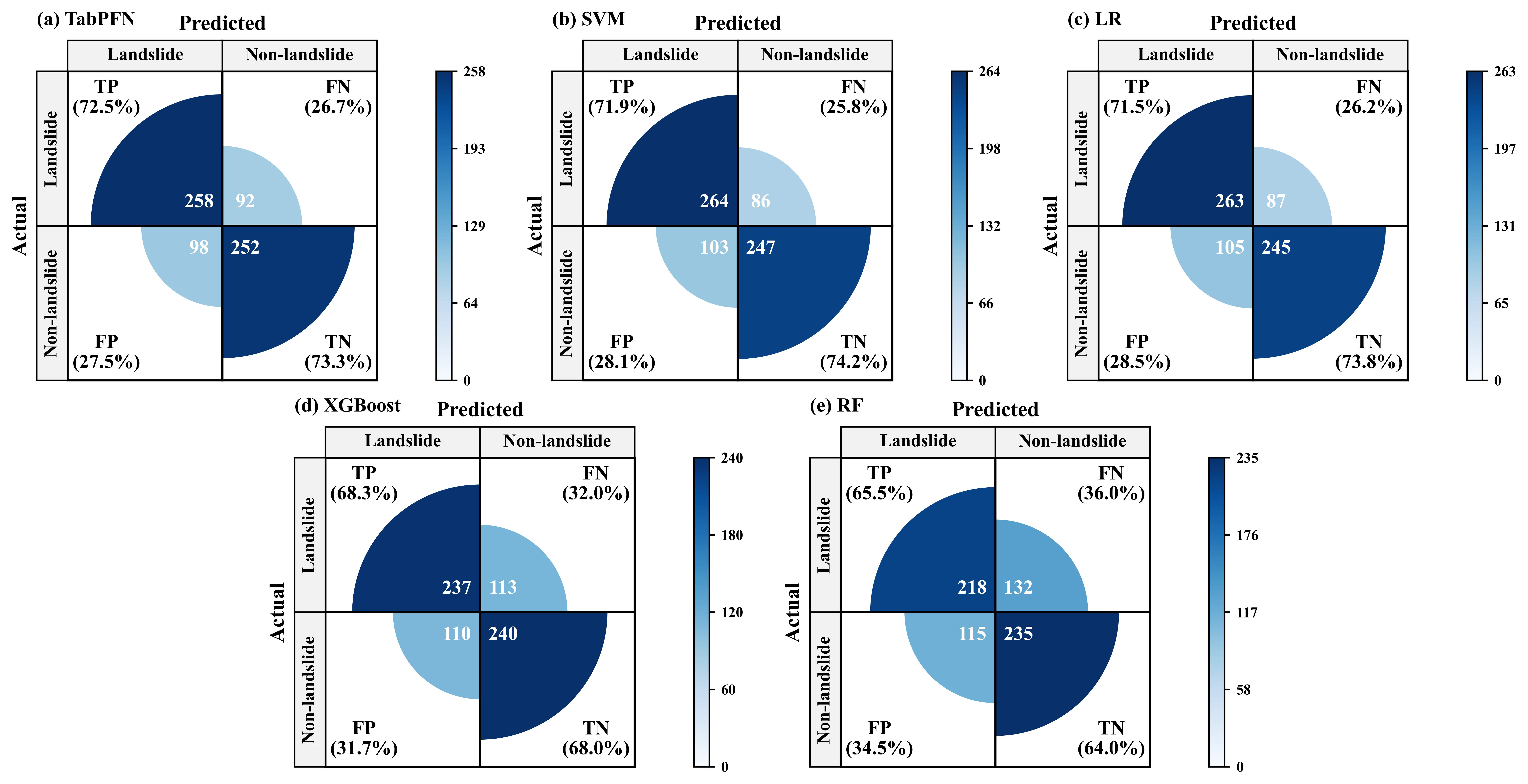
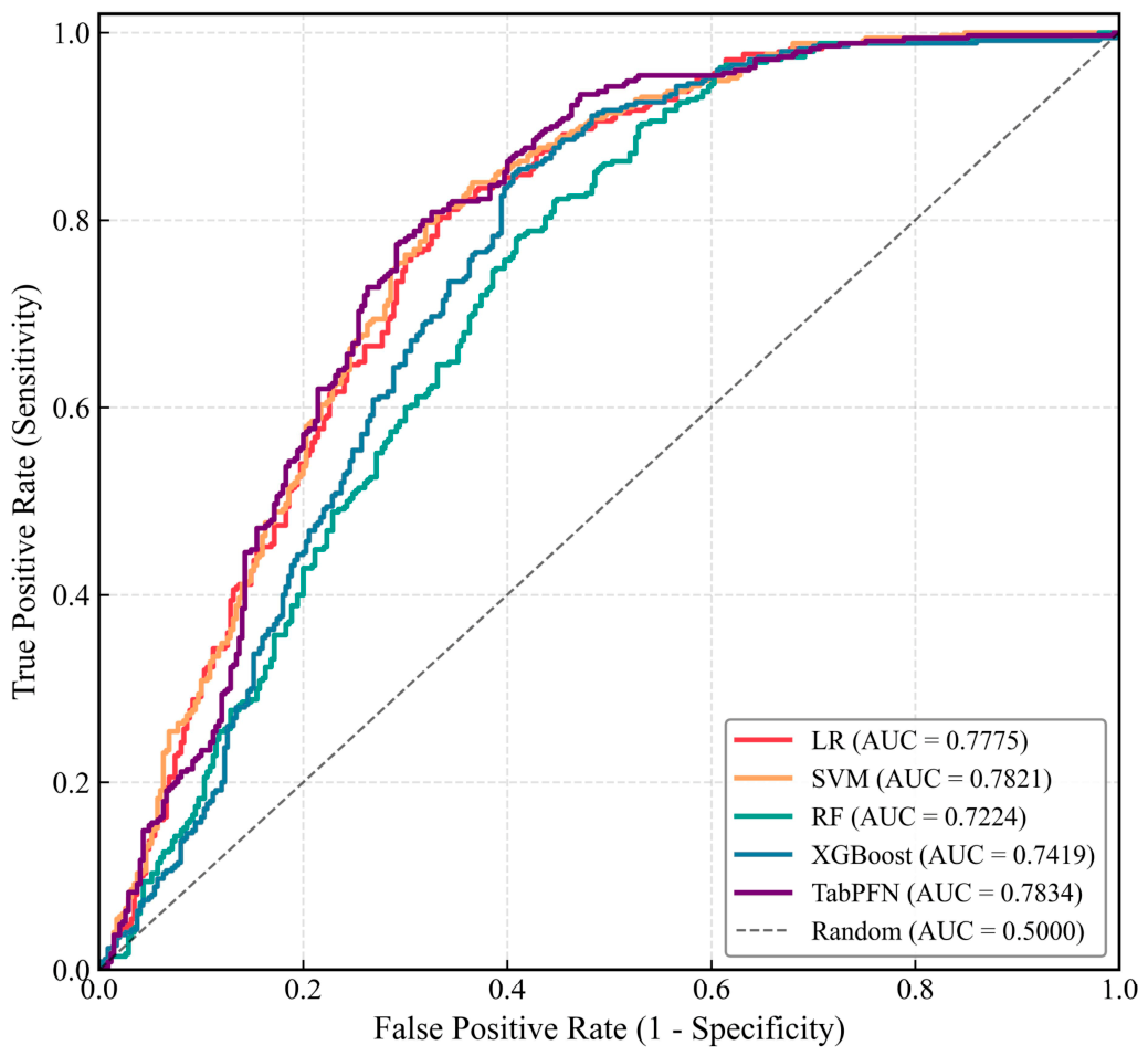
To quantify the performance of different machine learning models in landslide susceptibility assessment in Qingchuan County, confusion matrices were calculated in this study (Figure 7), from which accuracy, precision, recall, and F1-score were derived. These metrics were further combined with the receiver operating characteristic (ROC) curve to evaluate the predictive performance of the models. As shown in Figure 8, the AUC values of the five models, namely LR, SVM, RF, XGBoost, and TabPFN, were 0.7775, 0.7821, 0.7224, 0.7419, and 0.7834, respectively, all exceeding 0.7. This indicated that the five models had acceptable fitting and prediction capabilities and could effectively identify and classify landslide susceptibility in Qingchuan County.

To compare the discriminatory performance of different models, pairwise DeLong tests were performed based on the out-of-fold predicted probabilities to compare the AUCs (

Table 2. DeLong Test Results.

Model 1	Model 2	AUC 1	AUC 2	AUC Difference	p-Value
LR	SVM	0.7775	0.7821	−0.0046	0.3850
LR	RF	0.7775	0.7224	0.0551	<0.0001
LR	XGBoost	0.7775	0.7419	0.0356	0.0009
LR	TabPFN	0.7775	0.7834	−0.0059	0.4891
SVM	RF	0.7821	0.7224	0.0596	<0.0001
SVM	XGBoost	0.7821	0.7419	0.0401	0.0003
SVM	TabPFN	0.7821	0.7834	−0.0013	0.8751
RF	XGBoost	0.7224	0.7419	−0.0195	0.0493
RF	TabPFN	0.7224	0.7834	−0.0609	<0.0001
XGBoost	TabPFN	0.7419	0.7834	−0.0415	<0.0001

). TabPFN achieved the highest AUC (0.7834), followed by SVM (0.7821) and LR (0.7775), whereas XGBoost (0.7419) and RF (0.7224) showed relatively lower AUC values. The pairwise comparisons showed that the AUC differences among TabPFN, SVM, and LR were not statistically significant (TabPFN vs. SVM: AUC difference = 0.0013, p = 0.8751; TabPFN vs. LR: AUC difference = 0.0059, p = 0.4891; SVM vs. LR: AUC difference = 0.0046, p = 0.3850). These results indicate that the three models had comparable discriminatory ability. Although TabPFN achieved the numerically highest AUC, its improvement over SVM and LR did not reach statistical significance. The AUC of RF was significantly lower than those of LR, SVM, and TabPFN, with AUC differences of 0.0551, 0.0596, and 0.0609, respectively (all p < 0.0001). Similarly, XGBoost showed significantly lower AUC values than LR, SVM, and TabPFN, with AUC differences of 0.0356 (p = 0.0009), 0.0401 (p = 0.0003), and 0.0415 (p < 0.0001), respectively. In addition, XGBoost achieved a higher AUC than RF by 0.0195, and this difference was statistically significant before multiple-comparison correction (p = 0.0493).

Overall, TabPFN, SVM, and LR demonstrated relatively high and comparable discriminatory performance. XGBoost showed intermediate performance, whereas RF exhibited comparatively weaker discriminatory ability.

To further evaluate the stability of model performance, the AUC values obtained from the validation folds of the five-fold spatial cross-validation within the training dataset were summarized as mean ± standard deviation. As shown in

Table 3. AUC variation across five-fold spatial cross-validation within the training dataset.

Model	Spatial CV AUC, Mean ± SD
LR	0.7923 ± 0.0755
SVM	0.7877 ± 0.0707
RF	0.7542 ± 0.0938
XGBoost	0.7587 ± 0.0716
TabPFN	0.8039 ± 0.1020

, the TabPFN model achieved the highest mean AUC, followed by LR, SVM, XGBoost, and RF. These results indicate the variation in model performance across different spatial validation folds during internal cross-validation.

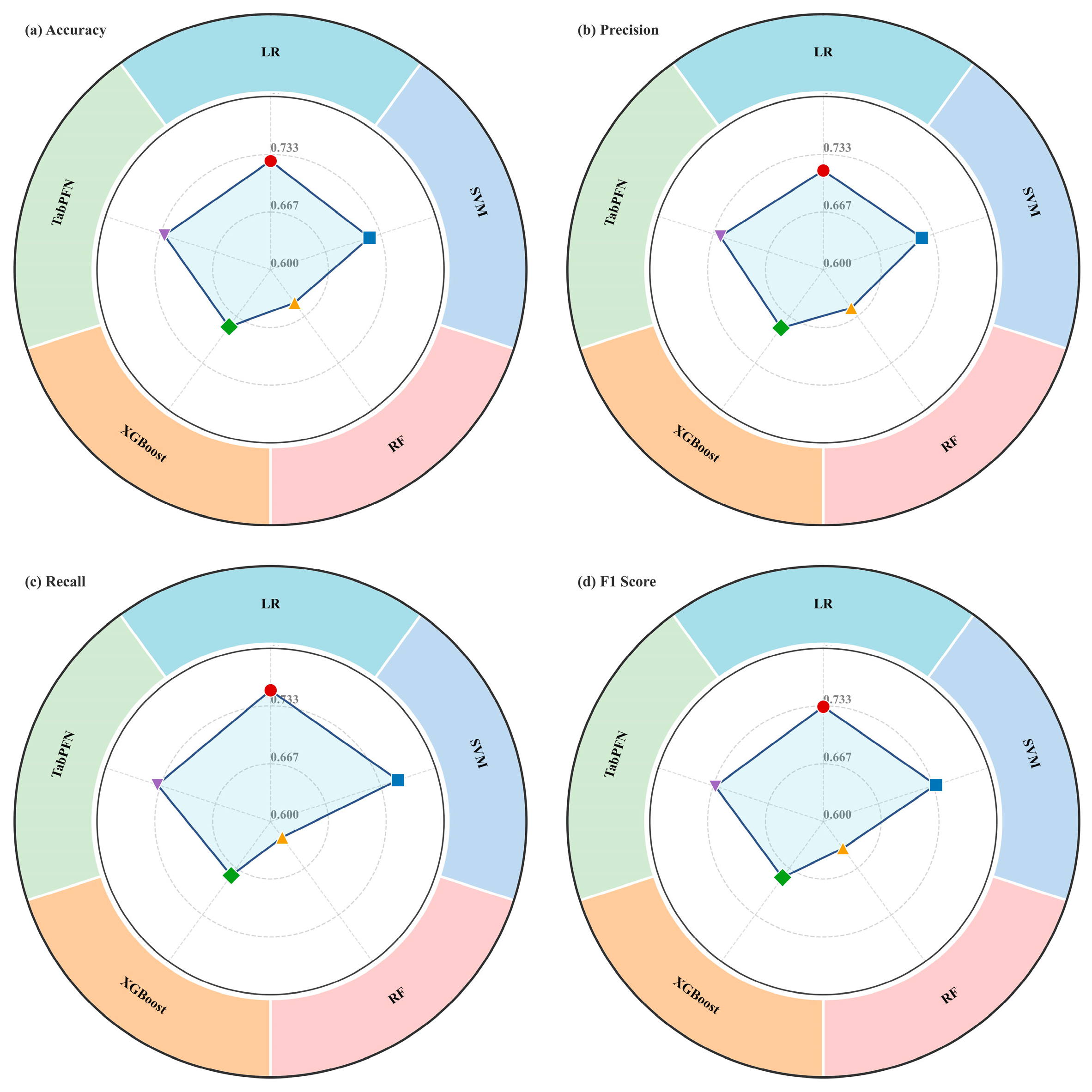
In addition, Figure 9 and

Table 4. Specific values of performance metrics.

Model	Accuracy	Precision	Recall	F1 Score
LR	0.723	0.715	0.751	0.733
SVM	0.730	0.719	0.754	0.736
RF	0.647	0.655	0.623	0.638
XGBoost	0.681	0.683	0.677	0.680
TabPFN	0.729	0.725	0.737	0.731

showed that the TabPFN model exhibited strong and well-balanced classification performance across the four evaluation metrics. Although SVM achieved the highest accuracy (0.730), TabPFN obtained a very similar accuracy value (0.729), with only a marginal difference of 0.001, indicating that TabPFN maintained a high level of overall classification accuracy. More importantly, TabPFN achieved the highest precision (0.725) among the five models, outperforming SVM (0.719), LR (0.715), XGBoost (0.683), and RF (0.655). Given the small difference between TabPFN and SVM, this result suggests only a marginal advantage of TabPFN in reducing false-positive predictions, rather than a definitive superiority over the other models. In terms of recall, TabPFN achieved a value of 0.737, which was slightly lower than those of SVM (0.754) and LR (0.751), but still indicated good capability in identifying actual landslide samples. With respect to the F1-score, TabPFN obtained a value of 0.731, which was close to those of SVM (0.736) and LR (0.733), suggesting that TabPFN maintained competitive comprehensive classification performance while achieving the highest precision. In comparison, XGBoost showed moderate performance, whereas RF had relatively lower values for accuracy, recall, and F1-score, indicating weaker overall classification ability. Overall, TabPFN showed a distinct advantage in precision and maintained high accuracy and F1-score values, demonstrating its effectiveness and stability for landslide susceptibility classification.

5. Discussion

5.1. Analysis of LSM Results

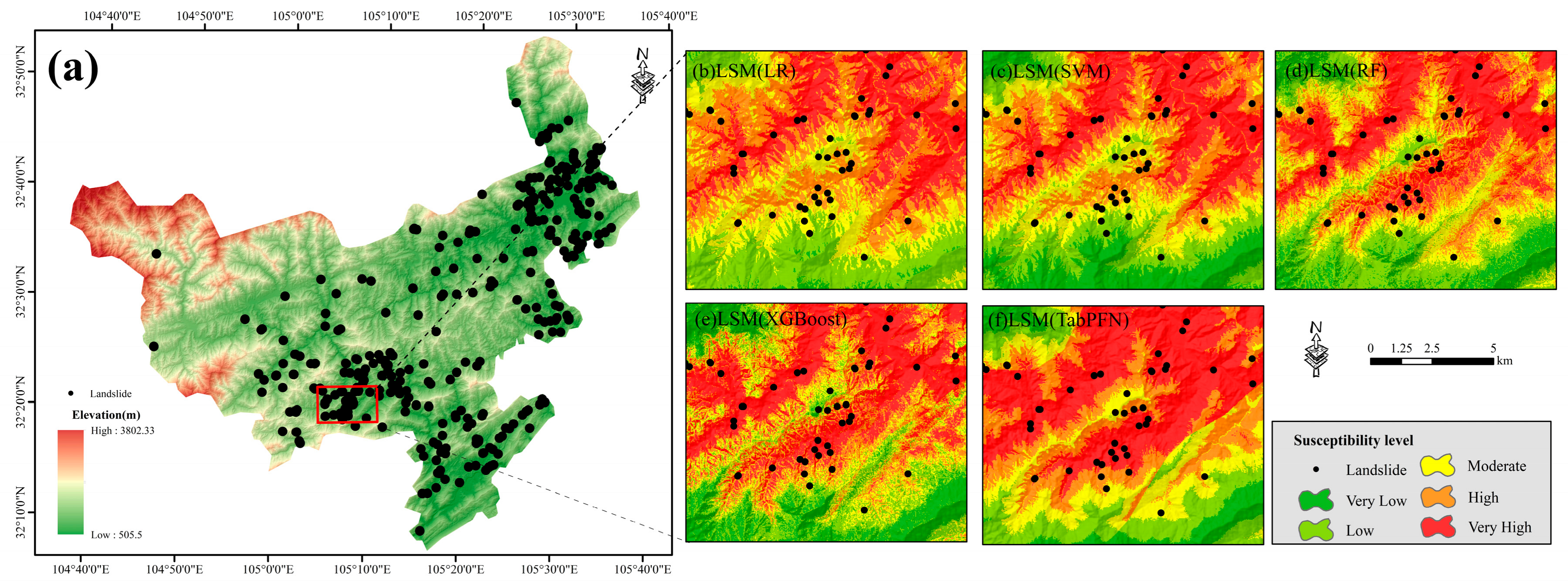
Figure 10 presents the distribution of historical landslides, the elevation profile of the study area, and enlarged sections of susceptibility maps produced by various models for the selected region. As indicated by the elevation pattern and landslide distribution in Figure 10a, landslide occurrences are not mainly clustered in high-elevation areas; instead, they are more frequently found across low- and middle-elevation belts. The enlarged views in Figure 10b–f show that TabPFN delineates high-susceptibility zones well, with most landslide locations located within the very high- and high-susceptibility areas. This indicates that TabPFN captures the spatial clustering tendency of landslides in complex terrain to some extent. The other models show broadly similar spatial patterns, although some landslide locations are not covered by the highest-susceptibility zones. Overall, TabPFN demonstrates a marginal advantage in identifying landslide-prone areas, rather than a clearly superior capability.

5.2. SHAP-Based Explainability of TabPFN Model Predictions

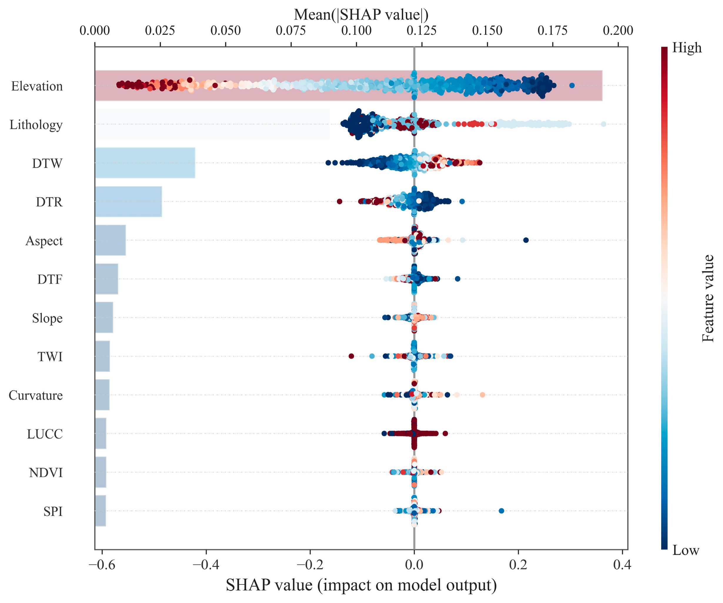
Different conditioning factors have distinct effects on landslide occurrence. To reveal the contribution of each factor to the model output, SHAP interpretability analysis is conducted on the optimal TabPFN model. As shown in Figure 11, elevation is the dominant conditioning factor, while lithology and DTR are secondary factors. Their contributions to the model predictions are significantly higher than those of the other factors. By calculating the mean absolute SHAP value of each feature, the feature importance plot is generated. Elevation, lithology, and DTR rank as the top three factors in terms of both contribution and importance, which is consistent with the SHAP value results.

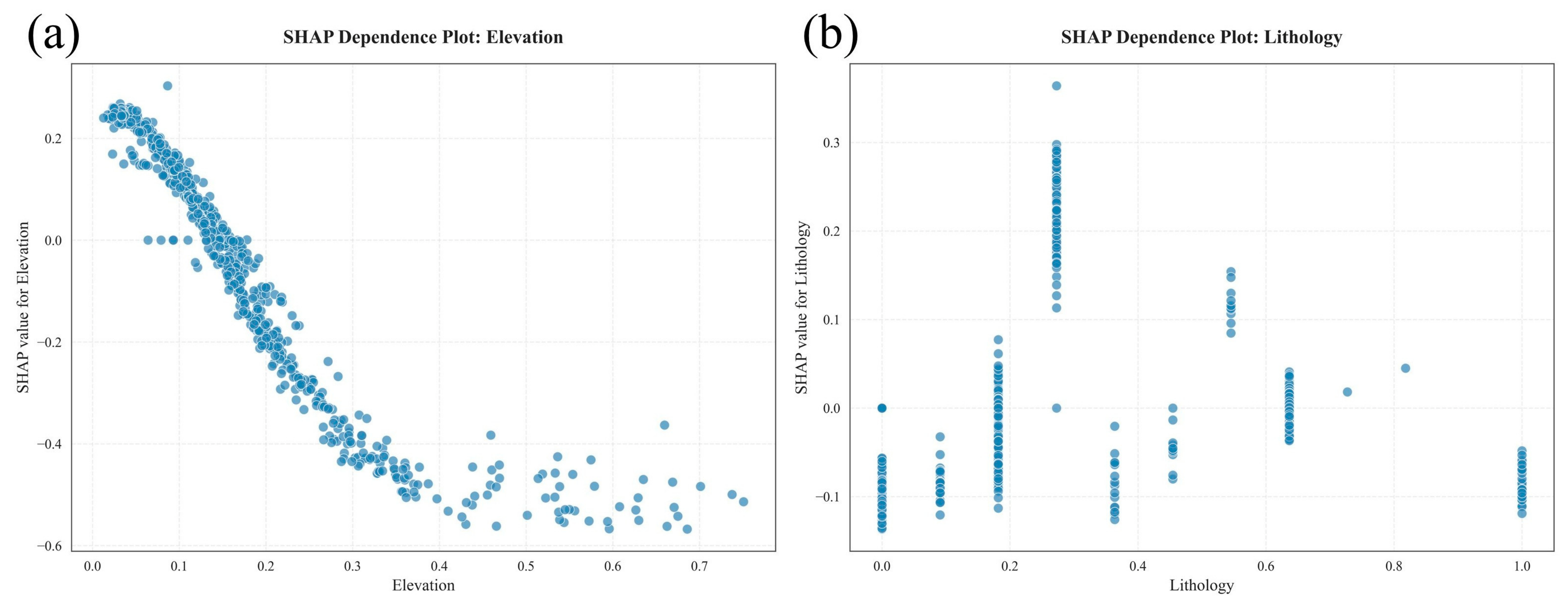
Nevertheless, factor-importance results alone are insufficient to fully verify the geomorphological soundness of the model [37]. Therefore, SHAP dependence plots were further used to examine the response patterns of the main conditioning factors and to clarify their geomorphic implications (Figure 12). For elevation, the SHAP results show that low- to moderate-altitude zones, ranging from 505 to 1300 m, contribute markedly to higher landslide susceptibility, while areas above 1700 m generally show a pronounced negative influence. This pattern is consistent with the landslide distribution in the study area, where landslide locations are mainly concentrated in low-elevation river valleys and foothill areas at 505–1300 m. These areas are strongly affected by river erosion, artificial slope cutting, and engineering activities. They are characterized by thick alluvial deposits and fragmented terrain, making them highly prone to landslides. In contrast, high-elevation areas above 1700 m show relatively intact terrain and high vegetation coverage, with generally good slope stability, resulting in a significantly lower probability of landslide occurrence. For lithology, it should first be noted that lithology is a categorical variable, and there is no inherent ordinal relationship among different lithological classes. To avoid imposing an artificial numerical order on lithological categories, one-hot encoding was applied to transform lithology prior to its use as a model input in this study. Accordingly, the SHAP analysis results for lithology should be interpreted as the contribution of each lithological class to model predictions relative to the reference condition, rather than responses along a continuous lithological gradient. Based on this interpretation, specific weak lithological units contribute significantly to landslide susceptibility, whereas hard and intact bedrock units show a clear negative contribution. This reflects the different controls of rock shear strength and weathering degree on slope stability. From the perspective of spatial distribution, landslide locations are highly concentrated in strip-like areas where weak lithologies are exposed, while the number of landslides in bedrock areas is notably lower, which is highly consistent with the geological setting.

5.3. Comparative Analysis of Models

Different evaluation models perform differently in the same study area. In this study, five models, including LR, SVM, RF, XGBoost, and TabPFN, are selected to assess landslide susceptibility in Qingchuan County. The results show that the AUC value of the TabPFN model (0.7834) is higher than those of the other four models by 0.0059, 0.0013, 0.0609, and 0.0415, respectively. In addition, TabPFN achieved the highest precision among the five models, while its accuracy and F1-score were very close to those of SVM and LR, indicating strong and well-balanced classification performance. This indicates that the TabPFN model showed a distinct advantage in reducing false-positive predictions and maintained highly competitive overall predictive performance in the Qingchuan case, providing a more accurate delineation of high-risk landslide zones and a higher degree of spatial agreement with actual landslide locations. It should be noted that this result differs from the finding of Zhou et al. (2025) [19], in which RF performed better than TabPFN. This discrepancy suggests that the performance advantage of TabPFN is not universal but may be affected by differences in study-area characteristics, landslide inventory composition, sample size, conditioning factors, model settings, and validation strategies. Therefore, the superior performance of TabPFN observed in this study should be interpreted within the specific geomorphological, geological, and data conditions of Qingchuan County.

Furthermore, owing to its Transformer architecture and contextual learning mechanism, the TabPFN model can rapidly capture the nonlinear coupling relationships among multiple landslide conditioning factors without extensive hyperparameter tuning. It maintains stable and efficient predictive performance even under limited data conditions, making it particularly suitable for assessment scenarios involving limited geological hazard samples and complex conditioning factors. Although the RF and XGBoost models show robust performance, they are inferior to TabPFN in overall AUC performance and precision-based classification reliability. The LR model has a simple structure and high interpretability, but it has difficulty capturing complex nonlinear relationships. The SVM model achieved high accuracy and recall, but its precision was slightly lower than that of TabPFN, suggesting a relatively higher tendency toward false-positive prediction.

Overall, the TabPFN model achieved the highest AUC value among the evaluated models and showed the most prominent precision advantage together with stable comprehensive performance, indicating its potential applicability for landslide susceptibility assessment in Qingchuan County.

5.4. Limitations and Future Work

Qingchuan County is located within the Longmen Shan seismic belt, which is characterized by highly fractured bedrock and a dense fault network, making it prone to structurally controlled regional landslides. This study uses geological factors, such as lithology and DTF, as independent evaluation factors for landslide susceptibility assessment. However, this approach has difficulty fully reflecting the development mechanisms of landslides under structural control and does not deeply investigate the connectivity and spatial relationships among these factors. Furthermore, although the TabPFN model demonstrates excellent performance in landslide susceptibility assessment, historical seismic and rainfall events are not incorporated into the susceptibility analysis. In particular, Qingchuan County was strongly affected by the 2008 Wenchuan earthquake (Mw 7.9), and the landslide inventory used in this study may contain pre-earthquake, co-seismic, and post-earthquake landslides. Due to the lack of reliable occurrence dates for individual landslides, event-based stratified modeling could not be conducted in this study. Consequently, the model has difficulty capturing the response characteristics of landslide susceptibility under extreme disaster events, and dynamic assessment requires further research.

In the future, efforts should focus on enriching the diversity of evaluation factors and conducting in-depth studies on the connectivity among these factors to improve the predictive accuracy and validity of the model. Future studies should establish time-specific landslide inventories, incorporate rainfall, seismic activity, population density, and other human-activity-related variables, and develop event-based or temporally stratified susceptibility models to reduce potential seismic-related confounding and better distinguish intrinsic terrain susceptibility from earthquake-induced landslide effects. In addition, future research should further explore the connectivity and spatial relationships among evaluation factors, and the proposed framework should be tested in other regions with different geological, geomorphological, climatic, and socio-economic conditions to evaluate its transferability and general applicability.

6. Conclusions

This study evaluated landslide susceptibility in Qingchuan County using five models, namely LR, RF, SVM, XGBoost, and TabPFN. By integrating model performance evaluation with SHAP-based interpretability analysis, this study identified the spatial distribution characteristics and key controlling factors of landslides in the region and compared the predictive performance of different models. It should be noted that the machine-learning-based susceptibility results are mainly intended for preliminary regional-scale risk identification and cannot replace detailed site-scale slope stability analysis. For specific slopes, the final stability assessment should be confirmed through appropriate geotechnical investigation and stability analysis. The main conclusions are as follows:

(1)

The landslide susceptibility zones in Qingchuan County exhibited a spatial distribution pattern characterized by higher susceptibility in the central and southeastern regions and lower susceptibility in the northwestern region. The very high- and high-susceptibility zones were distributed in a strip-like pattern along rivers and major transportation routes, which was highly consistent with the actual distribution of landslide sites.

(2)

The comparison results of the five models showed that the TabPFN model achieved the highest AUC value of 0.7834, which was higher than those of the LR model (AUC = 0.7775), RF model (AUC = 0.7224), SVM model (AUC = 0.7821), and XGBoost model (AUC = 0.7419). The TabPFN model achieved the highest precision among the five models, while maintaining accuracy and F1-score values comparable to those of SVM and LR. This indicates that TabPFN has an advantage in reducing false-positive predictions and provides stable overall classification performance. Therefore, it was more suitable for landslide susceptibility assessment in the complex geological environment of Qingchuan County.

(3)

Based on the SHAP interpretability analysis, the contribution rates and relative importance of 12 evaluation factors in the landslide susceptibility assessment model were quantified. Elevation, lithology, and DTR were ranked as the top three factors in the SHAP importance analysis of landslide occurrence in Qingchuan County. Specifically, areas with low to medium elevation, weak lithology, and proximity to roads were more prone to landslides. The combined effect of these three factors further increased landslide susceptibility.

References

1. Tehrani, F.S.; Calvello, M.; Liu, Z.; Zhang, L.; Lacasse, S. Machine Learning and Landslide Studies: Recent Advances and Applications. Nat. Hazards 2022, 114, 1197–1245. [Google Scholar] [CrossRef]
2. Huang, F.; Xiong, H.; Jiang, S.-H.; Yao, C.; Fan, X.; Catani, F.; Chang, Z.; Zhou, X.; Huang, J.; Liu, K. Modelling Landslide Susceptibility Prediction: A Review and Construction of Semi-Supervised Imbalanced Theory. Earth-Sci. Rev. 2024, 250, 104700. [Google Scholar] [CrossRef]
3. Wang, H.; Zhang, L.; Luo, H.; He, J.; Cheung, R.W.M. AI-Powered Landslide Susceptibility Assessment in Hong Kong. Eng. Geol. 2021, 288, 106103. [Google Scholar] [CrossRef]
4. Panchal, S.; Shrivastava, A.K. Landslide Hazard Assessment Using Analytic Hierarchy Process (AHP): A Case Study of National Highway 5 in India. Ain Shams Eng. J. 2022, 13, 101626. [Google Scholar] [CrossRef]
5. Lu, J.; Ma, G.; Zhang, G. Fuzzy Machine Learning: A Comprehensive Framework and Systematic Review. IEEE Trans. Fuzzy Syst. 2024, 32, 3861–3878. [Google Scholar] [CrossRef]
6. Yuan, X.; Liu, C.; Nie, R.; Yang, Z.; Li, W.; Dai, X.; Cheng, J.; Zhang, J.; Ma, L.; Fu, X.; et al. A Comparative Analysis of Certainty Factor-Based Machine Learning Methods for Collapse and Landslide Susceptibility Mapping in Wenchuan County, China. Remote Sens. 2022, 14, 3259. [Google Scholar] [CrossRef]
7. Guo, Z.; Shi, Y.; Huang, F.; Fan, X.; Huang, J. Landslide Susceptibility Zonation Method Based on C5.0 Decision Tree and K-Means Cluster Algorithms to Improve the Efficiency of Risk Management. Geosci. Front. 2021, 12, 101249. [Google Scholar] [CrossRef]
8. Zhao, P.; Wang, Y.; Xie, Y.; Uddin, M.G.; Xu, Z.; Chang, X.; Zhang, Y. Landslide Susceptibility Assessment Using Information Quantity and Machine Learning Integrated Models: A Case Study of Sichuan Province, Southwestern China. Earth Sci. Inform. 2025, 18, 190. [Google Scholar] [CrossRef]
9. Tay, J.K.; Narasimhan, B.; Hastie, T. Elastic Net Regularization Paths for All Generalized Linear Models. J. Stat. Softw. 2023, 106, 1–31. [Google Scholar] [CrossRef] [PubMed]
10. Zabor, E.C.; Reddy, C.A.; Tendulkar, R.D.; Patil, S. Logistic Regression in Clinical Studies. Int. J. Radiat. Oncol. Biol. Phys. 2022, 112, 271–277. [Google Scholar] [CrossRef] [PubMed]
11. Al-Najjar, H.A.H.; Pradhan, B.; Beydoun, G.; Sarkar, R.; Park, H.-J.; Alamri, A. A Novel Method Using Explainable Artificial Intelligence (XAI)-Based Shapley Additive Explanations for Spatial Landslide Prediction Using Time-Series SAR Dataset. Gondwana Res. 2023, 123, 107–124. [Google Scholar] [CrossRef]
12. Sharma, N.; Saharia, M.; Ramana, G.V. High Resolution Landslide Susceptibility Mapping Using Ensemble Machine Learning and Geospatial Big Data. CATENA 2024, 235, 107653. [Google Scholar] [CrossRef]
13. Kavzoglu, T.; Teke, A. Predictive Performances of Ensemble Machine Learning Algorithms in Landslide Susceptibility Mapping Using Random Forest, Extreme Gradient Boosting (XGBoost) and Natural Gradient Boosting (NGBoost). Arab. J. Sci. Eng. 2022, 47, 7367–7385. [Google Scholar] [CrossRef]
14. Guo, Z.; Tian, B.; Zhu, Y.; He, J.; Zhang, T. How Do the Landslide and Non-Landslide Sampling Strategies Impact Landslide Susceptibility Assessment?—A Catchment-Scale Case Study from China. J. Rock Mech. Geotech. Eng. 2024, 16, 877–894. [Google Scholar] [CrossRef]
15. Zhang, W.; He, Y.; Wang, L.; Liu, S.; Meng, X. Landslide Susceptibility Mapping Using Random Forest and Extreme Gradient Boosting: A Case Study of Fengjie, Chongqing. Geol. J. 2023, 58, 2372–2387. [Google Scholar] [CrossRef]
16. Wang, H.; Deng, C.; Zhang, Z.; Jiang, Z.; Wei, Q.; Yi, W.; Chen, T.; Ma, J. Dynamic Landslide Susceptibility Assessment Integrating SBAS-InSAR and Interpretable Machine Learning: A Case Study of the Baihetan Reservoir Area, Southwest China. Remote Sens. 2026, 18, 578. [Google Scholar] [CrossRef]
17. Tran, V.Q.; Byeon, H. Predicting Dementia in Parkinson’s Disease on a Small Tabular Dataset Using Hybrid LightGBM-TabPFN and SHAP. Digit. Health 2024, 10, 20552076241272585. [Google Scholar] [CrossRef] [PubMed]
18. Schmidinger, J.; Barkov, V.; Vogel, S.; Atzmueller, M.; Heuvelink, G.B.M. Kriging Prior Regression: A Case for Kriging-Based Spatial Features with TabPFN in Soil Mapping. Comput. Electron. Agric. 2026, 243, 111352. [Google Scholar] [CrossRef]
19. Zhou, Y.; Xue, L.; Ding, H.; Wang, H.; Huang, K.; Li, L.; Li, Z. Landslide Risk Assessment as a Reference for Disaster Prevention and Mitigation: A Case Study of the Renhe District, Panzhihua City, China. Remote Sens. 2025, 17, 2120. [Google Scholar] [CrossRef]
20. Huang, J.; Zeng, X.; Ding, L.; Yin, Y.; Li, Y. Landslide Susceptibility Evaluation Using Different Slope Units Based on BP Neural Network. Comput. Intell. Neurosci. 2022, 2022, 9923775. [Google Scholar] [CrossRef] [PubMed]
21. Luo, Y.; Zhang, Y.; Wang, Y.; He, Y.; Zhang, Y.; Cao, H. A Unique Failure Model for a Landslide Induced by the Wenchuan Earthquake in the Liujiawan Area, Qingchuan County, China. Eng. Geol. 2021, 295, 106412. [Google Scholar] [CrossRef]
22. Zhang, J.; Ma, X.; Zhang, J.; Sun, D.; Zhou, X.; Mi, C.; Wen, H. Insights into Geospatial Heterogeneity of Landslide Susceptibility Based on the SHAP-XGBoost Model. J. Environ. Manag. 2023, 332, 117357. [Google Scholar] [CrossRef] [PubMed]
23. Lin, N.; Zhang, D.; Feng, S.; Ding, K.; Tan, L.; Wang, B.; Chen, T.; Li, W.; Dai, X.; Pan, J.; et al. Rapid Landslide Extraction from High-Resolution Remote Sensing Images Using SHAP-OPT-XGBoost. Remote Sens. 2023, 15, 3901. [Google Scholar] [CrossRef]
24. Pate, A.; Riley, R.D.; Collins, G.S.; van Smeden, M.; Van Calster, B.; Ensor, J.; Martin, G.P. Minimum Sample Size for Developing a Multivariable Prediction Model Using Multinomial Logistic Regression. Stat. Methods Med. Res. 2023, 32, 555–571. [Google Scholar] [CrossRef] [PubMed]
25. Wu, M.; Si, J.; Liu, Y.; Kang, L.; Xu, B. Association between Composite Dietary Antioxidant Index and Hypertension: Insights from NHANES. Clin. Exp. Hypertens. 2023, 45, 2233712. [Google Scholar] [CrossRef] [PubMed]
26. Sun, Z.; Wang, G.; Li, P.; Wang, H.; Zhang, M.; Liang, X. An Improved Random Forest Based on the Classification Accuracy and Correlation Measurement of Decision Trees. Expert Syst. Appl. 2024, 237, 121549. [Google Scholar] [CrossRef]
27. Rhodes, J.S.; Cutler, A.; Moon, K.R. Geometry- and Accuracy-Preserving Random Forest Proximities. IEEE Trans. Pattern Anal. Mach. Intell. 2023, 45, 10947–10959. [Google Scholar] [CrossRef] [PubMed]
28. Wiens, M.; Verone-Boyle, A.; Henscheid, N.; Podichetty, J.T.; Burton, J. A Tutorial and Use Case Example of the eXtreme Gradient Boosting (XGBoost) Artificial Intelligence Algorithm for Drug Development Applications. Clin. Transl. Sci. 2025, 18, e70172. [Google Scholar] [CrossRef] [PubMed]
29. Mienye, I.D.; Sun, Y. A Survey of Ensemble Learning: Concepts, Algorithms, Applications, and Prospects. IEEE Access 2022, 10, 99129–99149. [Google Scholar] [CrossRef]
30. Song, Y.; Huang, Z.; Jin, M.; Liu, Z.; Wang, X.; Hou, C.; Zhang, X.; Shen, Z.; Zhang, Y. Machine Learning Prediction of Biochar Physicochemical Properties Based on Biomass Characteristics and Pyrolysis Conditions. J. Anal. Appl. Pyrolysis 2024, 181, 106596. [Google Scholar] [CrossRef]
31. Malashin, I.; Tynchenko, V.; Gantimurov, A.; Nelyub, V.; Borodulin, A. Support Vector Machines in Polymer Science: A Review. Polymers 2025, 17, 491. [Google Scholar] [CrossRef] [PubMed]
32. Roy, A.; Chakraborty, S. Support Vector Machine in Structural Reliability Analysis: A Review. Reliab. Eng. Syst. Saf. 2023, 233, 109126. [Google Scholar] [CrossRef]
33. Tanveer, M.; Rajani, T.; Rastogi, R.; Shao, Y.H.; Ganaie, M.A. Comprehensive Review on Twin Support Vector Machines. Ann. Oper. Res. 2024, 339, 1223–1268. [Google Scholar] [CrossRef]
34. Hollmann, N.; Müller, S.; Purucker, L.; Krishnakumar, A.; Körfer, M.; Hoo, S.B.; Schirrmeister, R.T.; Hutter, F. Accurate Predictions on Small Data with a Tabular Foundation Model. Nature 2025, 637, 319–326. [Google Scholar] [CrossRef] [PubMed]
35. Pal, S.C.; Biswas, T.; Ghorai, S.; Pande, C.B.; Islam, A.; Islam, A.R.M.T.; Alam, E. Landslide Vulnerability Mapping Using GIS-Based Statistical Model for Sustainable Ecosystem Management in the Himalayan Region of Teesta River Basin, India. Environ. Sci. Eur. 2025, 37, 60. [Google Scholar] [CrossRef]
36. Ma, T.; Yi, X.; Ci, H.; Wang, R.; Yang, H.; Yan, Z. Landslide Susceptibility Evaluation Integrating Machine Learning and SBAS-InSAR-Derived Deformation Characteristics: A Case Study of Yining County, Xinjiang. Sensors 2026, 26, 707. [Google Scholar] [CrossRef] [PubMed]
37. Yao, Y.; Du, Y.; Zhang, W.; Liu, X.; Cai, J.; Feng, H.; Xiang, H.; Hu, R.; Yang, Y.; Fu, T. Landslide Susceptibility Assessment Based on a Deep Learning-Derived Landslide Inventory in Moxi Town, Sichuan, China. Remote Sens. 2026, 18, 849. [Google Scholar] [CrossRef]
Figure 1. Study area: (a,b) Location map of the study area; (c) the Distribution of Landslides and Water Systems.
Applsci 16 07860 g001
Figure 2. Flowchart of the methodological framework used in this study.
Applsci 16 07860 g002
Figure 3. Spatial block assignment for spatial block cross-validation.
Applsci 16 07860 g003
Figure 4. Analysis of multicollinearity among factors.
Applsci 16 07860 g004
Figure 5. Thematic maps of factors: (a) elevation; (b) slope; (c) aspect; (d) curvature; (e) lithology; (f) DTF; (g) DTW; (h) TWI; (i) SPI; (j) LULC; (k) NDVI; (l) DTR.
Applsci 16 07860 g005
Figure 6. LSM of Qingchuan County: (a) LR model; (b) SVM model; (c) RF model; (d) XGBoost model; (e) TabPFN model.
Applsci 16 07860 g006
Figure 7. Confusion matrix of prediction results from different models: (a) LR model; (b) SVM model; (c) RF model; (d) XGBoost model; (e) TabPFN model.
Applsci 16 07860 g007
Figure 8. ROC curves for different landslide susceptibility assessment models.
Applsci 16 07860 g008
Figure 9. Performance of different models: (a) accuracy; (b) precision; (c) recall; (d) F1-score. The red circle, purple triangle, green diamond, blue square, and yellow triangle represent the LR, TabPFN, XGBoost, SVM, and RF models, respectively.
Applsci 16 07860 g009
Figure 10. Local enlarged view of Figure 5: (a) elevation and landslide information; (b) LR; (c) SVM; (d) RF; (e) XGBoost; (f) TabPFN.
Applsci 16 07860 g010
Figure 11. Feature importance and beeswarm distribution of the TabPFN model based on SHAP analysis.
Applsci 16 07860 g011
Figure 12. Dependence plots of key controlling factors for the TabPFN model based on SHAP analysis: (a) elevation; (b) lithology. Each blue dot corresponds to the SHAP value of an individual sample.
Applsci 16 07860 g012