Article

Prediction of Shear Strength of Silty Clay in Seasonally Frozen Regions Based on SSC-PINN

1
The Institute of Geological Survey of China University of Geosciences (Wuhan), Wuhan 430074, China
2
Faculty of Engineering, China University of Geosciences (Wuhan), Wuhan 430074, China
3
Survey and Design Institute of Xiangtan City, Xiangtan 411100, China
4
Harbin Center for Integrated Natural Resources Survey, China Geological Survey, Harbin 150081, China
5
Observation and Research Station of Earth Critical Zone in Black Soil Harbin, Ministry of Natural Resources, Harbin 150081, China
*
Author to whom correspondence should be addressed.
Appl. Sci. 2026, 16(15), 7746; https://doi.org/10.3390/app16157746
Submission received: 15 June 2026 / Revised: 22 July 2026 / Accepted: 30 July 2026 / Published: 4 August 2026

Abstract

The prediction of shear strength in seasonally frozen silty clay is restricted by complex physical mechanisms and sparse experimental data. A self-supervised contrastive physics-informed neural network is proposed to overcome these limitations. Robust latent features are extracted from limited datasets via contrastive pretraining. Time-dependent constitutive equations and physical boundary conditions are simultaneously embedded into the loss function. This mathematical constraint ensures strict physical consistency during the modeling process. The proposed framework was validated using 100 independent laboratory samples prepared under controlled moisture content, freezing temperature, and thawing duration. The experimental results demonstrate the superior predictive accuracy of the proposed model. A coefficient of determination ( R 2 ) of 0.988 was achieved on the test set, accompanied by minimized error metrics compared to conventional data-driven approaches. Consequently, a highly accurate and reliable methodology is established by this architecture for evaluating soil stability and supporting infrastructure design in cold regions.

1. Introduction

The seasonally frozen areas are distributed across the cold climate regions. Such regions are Northeastern and Northwestern China [1]. These areas are major regions in geotechnical engineering development. It is in these regions that unique climatic conditions produce repeated freeze–thaw cycles. The cycles cause changes in the physical and mechanical properties of soils [2]. There are different types of soils in these environments. Some of them are silty clay which has a complex behavior. These regions experience sub-zero temperatures. As a result, pore water is converted into ice masses. The freezing causes the development of ice lenses. In this step, cementation bonds also form [3]. The freezing action increases apparent cohesion as a result. Once thawed, the soil properties change. The residual unfrozen water films affect both their strength and deformation behavior. The matric suction also affects these mechanical properties. The shear strength of silty clay changes with several parameters. These parameters are moisture content, freezing temperature, and thawing duration. The variation is inherently highly non-linear [4].
Despite these understandings, what remains unresolved is that traditional empirical models have disadvantages, and purely data-driven methods cannot be used to completely characterize the system behavior [5]. The modeling process is complicated by non-homogeneous field conditions, sparse experimental data, and the underlying physics of ice-soil behavior. What makes this study novel is the introduction of a Self-Supervised Contrastive Physics-Informed Neural Network (SSC-PINN) to bridge the gap between physical modeling and representation learning. The objective of this study is to accurately predict the shear strength of seasonally frozen silty clay by embedding physical laws into the neural network to overcome the limitations of sparse data. The novel findings of this study will benefit geotechnical engineers and researchers by providing a reliable and robust computational tool for slope stability analysis and infrastructure design in cold regions.
The framework used in this study to fill this gap is called the Self-Supervised Contrastive PINN (SSC-PINN). This work has been divided into the following contributions:
  • Physics-informed data augmentation: Domain-specific augmentations produce positive and negative sample pairs. Such operations are able to account for measurement noise and environmental variation.
  • Contrastive pretraining module: An InfoNCE loss pretrains the encoder. The step creates embeddings that group similar physical conditions together and distinct ones apart. In turn, the approach improves the strength of features in case of sparse amounts of labeled data.
  • Integrated PINN regression: Network loss is based on classical constitutive laws and unsaturated soil boundary conditions. This is a restriction that makes predictions follow the principles of freeze–thaw mechanics.
  • Evaluation: The evaluation involved testing 100 laboratory samples using different levels of moisture, freezing temperature and thawing duration. As shown in the results, the SSC-PINN is superior to the standard PINNs and purely data-driven models. The model reduces RMSE and MAE and boosts R 2 . Moreover, the ablation experiments measure the separate effects of contrastive learning and physics-based constraints.
The primary objective of this research is explicitly established as the development and validation of a unified self-supervised contrastive physics-informed neural network framework. The accurate prediction of the shear strength degradation of seasonally frozen silty clay under cyclic thermal loading is specifically targeted by this advanced architecture. Furthermore, significant benefits are provided to geotechnical engineers, infrastructure planners, and disaster mitigation practitioners operating in cold regions by the novel findings of this study. The proposed predictive framework can be directly applied to regional landslide susceptibility mapping, the stability assessment of engineered slopes, and the design of resilient foundations in seasonal frost environments. Consequently, a robust micro mechanical and macro scale physical basis for the development of early warning systems for geohazards induced by cyclic freezing and thawing is explicitly provided by this research.

2. Background and Theoretical Foundations

2.1. Review of Related Research

Laboratory experiments have been traditionally used to measure the shear strength of soils [6]. Skempton and Bishop designed fundamental testing procedures [7]. Such procedures evaluate key shear strength variables in a controlled pore pressure dissipation environment. The parameters specifically are cohesion and the internal friction angle. Hongde et al. have studied coastal reclamation areas in China [8]. Their research focused on the relationship between unsaturated shear strength, soil salinity, and particle composition. The research has combined the use of direct shear tests and soil water characteristic curves. It was through this that the values of shear strength were obtained at 79 sampling points. Stefanow and Dudziński critically evaluated more than 20 methods of determining shear strength [9]. Their review pointed out the methodological differences between the methods. The review also considered the factors that led to the measurement variability. The methods are divided into forced-shear and free-shear plane methods [10]. The relationship between shear strength and soil detachability was investigated by Brunori et al. [11]. The study focused on how surface shear strength affects the erosion mechanisms. Such mechanisms are rill formation and splash detachment. Different measurement devices underwent a comparative analysis. There were Geonor cone penetrometer, laboratory vane tester, and pocket vane tester. The analysis showed dissimilarity in sensitivity and operation principles of the devices. Nam et al. developed a multistage direct shear test [12]. It is an alternative method to evaluate the shear strength of unsaturated soils. The method uses a suction-controlled apparatus to control matric suction. The comparative findings showed the estimates of unsaturated shear strength. These estimates are in line with the conventional approaches. Nevertheless, these experimental methods are associated with limitations [13]. The processes have extended testing times. They are also characterized by high operational costs. Moreover, these methods are also not responsive to rapid on-site assessments. Most traditional methods neglect dynamic environmental effects. Also, these methods do not consider the combined effects of various interacting factors. These factors directly influence the soil shear strength. Over the last few years, several modeling methods have been proposed to calculate the shear strength of soil and rock [14]. There are numerous studies that concentrate on empirical correlations that take into account environmental factors like temperature and water content [15]. As an illustration, the effect of temperature on the shear strength of saturated sand was investigated by Liu et al. [16]. Drained shear strength was experimentally correlated with liquid limit, clay size fraction, and effective normal stress by Stark and Hussain [17]. These formulations are applied in the course of slope stability analysis. Shear strength equations of unsaturated soils were suggested by Guan et al. [18]. Triaxial drained consolidated tests were carried out on the soils [19]. Empirical relations between rock strength and other factors were produced by Karakul and Ulusay [20]. The deviation is associated with lithology differences [21]. A Chinese study involved a tunnel construction project case study in Yunnan province [22]. A predictive model was used to quantify this behavior, grounded on the Joint Roughness Coefficient (JRC) and Joint Compressive Strength (JCS) criteria. Likewise, Pan et al. [23] explored the effects of freeze–thaw cycles. The research by Ping et al. [24] studied multiscale degradation of mudstone with gypsum.
Several constitutive models and empirical approaches have been created by researchers [25]. Cavalcante and Mascarenhas [26] offered a framework to describe the shear strength of unsaturated soils using the soil water retention curve (SWRC). Cai and Zhu [27] presented a constitutive model to describe saturated, partially frozen, cohesionless soils. The model explains the thermo-hydro-mechanical (THM) behavior of the soil. Pham and Sutman [28] created a shear strength equation of unsaturated soils. The formulation is based on the concept of disturbed states. Independently, Chen et al. [29] suggested a shear strength model of unsaturated frozen soils, using the unfrozen water content obtained through the soil freezing characteristic curve (SFCC) [30].
Physics-informed numerical schemes are used in geomechanical modeling [31]. Coupled thermo-hydro-mechanical (THM) finite element analyses are often used by researchers [32]. A physics-informed neural network (PINN) was proposed by Zhang et al. [33], which is called RheologyNet. The architecture embeds complex rheological partial differential equations (PDEs). Also, Amini et al. [34] have simulated the THM processes in porous media on the basis of PINNs. Rezaei et al. [35] also suggested a mixed-formulation PINN framework to address engineering issues in heterogeneous regions. At the same time, there is progress in self-supervised and contrastive learning demonstrating that networks can learn strong, noise-resistant feature embeddings. Yet, the existing literature cannot combine both self-supervised contrastive pretraining and PINNs in geotechnical engineering. The gap lies at the border of physical modeling and learning of representations. It indicates an open research direction.

2.2. Mechanisms of Shear Strength in Seasonally Frozen Silty Clay

The shear strength of seasonally frozen silty clay is governed by various physical mechanisms. These mechanisms include ice-induced cohesion and suction-enhanced frictional resistance. The viscous effects within the unfrozen water film also contribute to the overall resistance. Temperature determines the contribution of each mechanism. Temperature variations directly affect the ice content, suction magnitude, and water film viscosity. For this soil type, the total shear strength is formulated as a summation. This expression integrates the three major physical contributions:
τ = c ice + σ tan ϕ + τ viscous
where c ice is the apparent cohesion due to ice cementation, σ is the effective stress, ϕ is the friction angle, and τ viscous represents time-dependent viscous effects in the unfrozen water film [36].
As temperatures drop below freezing, pore water is transformed into ice [37]. During this phase transition, discrete ice bridges are formed between clay particles [38]. Thereby, tensile bonding forces are generated by these bridges. Such forces must be overcome before particle sliding is initiated, which fundamentally raises the apparent cohesion τ [39]. The strength of these ice bonds is directly affected by the saturation level, and the overall shear resistance is further scaled by the spatial continuity of the ice network. During slow freezing, water is induced to migrate toward the freezing front, causing segregated ice lenses to be formed [37]. Although a locally disruptive effect on the soil fabric is exerted by these lenses, overall shear resistance is provided by residual interlayer cementation. This resistance is preserved when the lenses remain intact during the shearing process [38].
Furthermore, as temperatures fall below the 0 °C mark, capillary and adsorptive forces are induced within the remaining unfrozen water [39]. Negative pore water pressure is created by this interaction. This geomechanical response is governed by the extended effective stress theory for unsaturated soils. The net normal stress at particle contacts is increased correspondingly with the escalation in matric suction. Consequently, the coefficient of frictional resistance tan ϕ is significantly enhanced [38].

2.3. Physics-Informed Neural Networks (PINNs): Principles and Formulations

The definition of Physics-informed neural networks (PINNs) is the incorporation of physical laws into the loss function of a neural network [40]. They are commonly expressed in the form of partial differential equations (PDEs) together with their respective boundary and initial conditions. This method aims at training a neural network surrogate u ( x ; θ ) , to represent the observed data as well as obey the underlying physical constraints.
N [ u ( x ; θ ) ] = 0
where N is a differential operator.
The modeling process uses a feed-forward network with trainable parameters. It takes input features of the input which could be spatial coordinates, time or other relevant state variables and produces an output prediction. Derivatives and higher-order terms are evaluated exactly through the automatic differentiation mechanism of the framework. This setup allows for evaluating the partial differential equation (PDE) residual directly without numerical discretization.
The total loss is a weighted sum of three terms:
L ( θ ) = λ data L data + λ phys L phys + λ bc L bc
Data loss:
L data = 1 N d i = 1 N d | u ( x i ; θ ) y i | 2
where { ( x i , y i ) } are measured sample points.
Physics loss:
L phys = 1 N c j = 1 N c | N [ u ( x j ; θ ) ] | 2
Evaluated at N c collocation points { x j } in the domain.
Boundary condition loss:
L bc = 1 N b k = 1 N b | u ( x k ; θ ) g k | 2
Enforcing u = g on known boundaries or initial surfaces.
The hyperparameters λ data , λ phys and λ bc are weighting coefficients that balance data fidelity against physical and boundary consistency. The rationale for their calibration and the specific values applied are detailed in Section 5.2.
The five phases that make up the training process of a Physics-Informed Neural Network (PINN) are described below. The five steps involved in the training process of a Physics-Informed Neural Network (PINN) are given below. Firstly, minibatches are chosen in each training iteration. They consist of observational data points, collocation points and boundary condition points. It is defined as the sampling step. Next, a forward pass is conducted.
The total loss is subsequently reconstructed from its constituent elements. This calculation takes place during the loss assessment phase. Backpropagation is subsequently executed. Gradients are calculated by automatic differentiation. Then, an optimization algorithm is used to update the network parameters. Finally, the convergence criteria terminate the training. This termination happens when the total loss plateaus. It may also be activated by the validation error falling below a given tolerance.
Precise predictions are facilitated by these methodological steps, even in cases where observational data are scarce or corrupted [41]. This robust capability is enabled by the combination of data-driven learning and the enforcement of governing physical laws. Strict constraints within the network are imposed by these physical laws. Consequently, the predictive model is successfully generalized to unseen scenarios within the investigated domain [42].

2.4. Overview of Self-Supervised Learning and Contrastive Learning

Data representations are acquired via self-supervised learning (SSL). The method operates without manually labeled datasets. Pretext tasks are introduced in this context. Such tasks are based on the automatic derivation of supervisory signals from the raw data itself. Subsequently, the model learns robust features that represent the underlying semantic and pattern structures. Upon completion of pretraining, the encoder is optimized to perform downstream tasks. This stage utilizes small labeled datasets. This training strategy ensures stable optimization in the presence of limited quantities of labeled data.
Contrastive learning represents a core variant of self-supervised learning. The encoders are trained in this context. The network structure aligns the representations of correlated views. At the same time, it segregates the representations of unrelated views. Four main components are generally incorporated into this architecture. They include data augmentation, an encoder, a contrastive loss function, and representation learning modules [43].
(1)
Data Augmentation: For each sample x , apply two stochastic augmentations to obtain views x ( 1 ) , x ( 2 ) . Augmentations should preserve underlying semantics, so that both views share the same label or physical condition.
(2)
Encoder: An encoder f θ maps each view to a latent representation h = f θ ( x ) Optionally, a small projection network g ϖ further maps h to a space z = g ϖ ( h ) where contrastive loss is applied.
(3)
Contrastive Loss: In a minibatch of N samples, each view z i ( 1 ) should be similar to its positive counterpart z i ( 2 ) and dissimilar to all other 2 ( N 1 ) negative views. The loss for one positive pair is:
L i = log exp ( s i m ( z i ( 1 ) , z i ( 2 ) ) / ς ) j = 1 N exp ( s i m ( z i ( 1 ) , z i ( 2 ) ) / ς )
where s i m ( ) is cosine similarity and ς is a temperature hyperparameter.
The encoder is trained to learn an embedding space. The optimization minimizes the average contrastive loss for all positive pairs. This procedure constitutes the core of representation learning. Within this space, the network clusters views that are associated with the same physical state. Conversely, the framework isolates different physical states.
In this study, the PINN encoder extracts specific features. These features are resilient to measurement noise while remaining sensitive to physically meaningful variations. This feature extraction process is facilitated by contrastive pretraining. As a result of this step, downstream shear strength predictions become more accurate.

3. Study Area and Data Acquisition

3.1. Field Site Description and Sampling

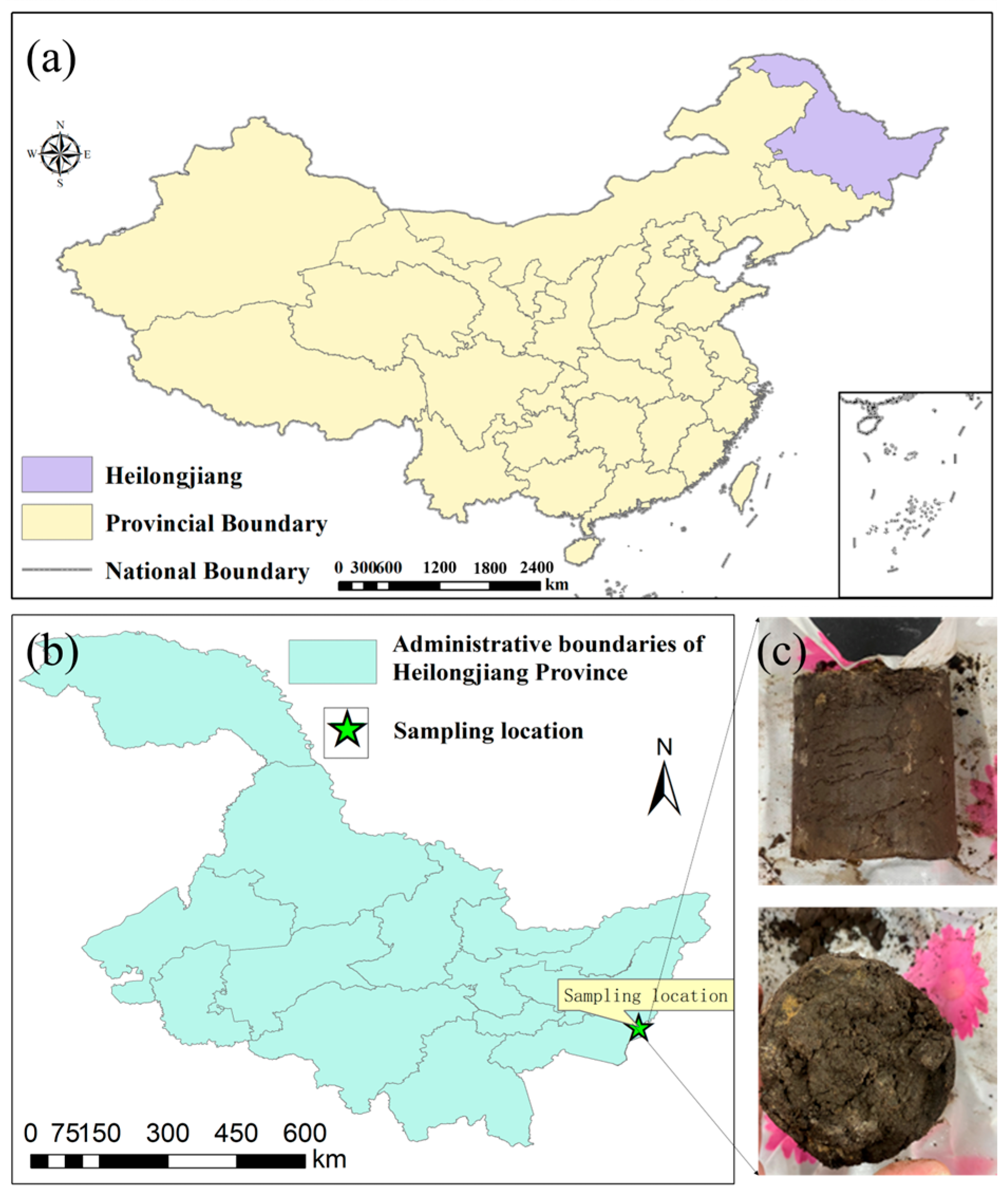
The soil samples utilized for the experimental testing were systematically collected from a seasonally frozen region located in Muling, Heilongjiang Province, China. A precise extraction depth of 2 m was strictly maintained during the field sampling procedure. The specific geographical location of the study area within Heilongjiang Province, alongside macroscopic visual representations of the undisturbed specimens, is explicitly illustrated in Figure 1. Furthermore, the initial physical and mechanical properties of the tested soil are comprehensively tabulated in Table 1.
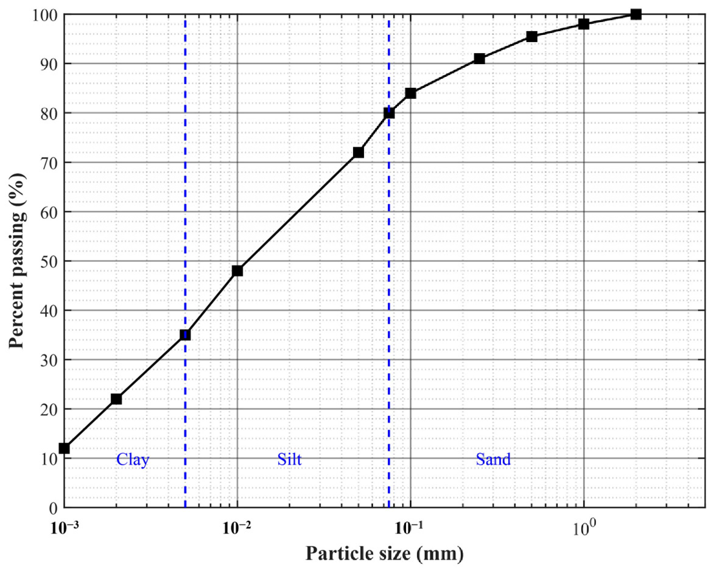
The soil samples were oven-dried and subsequently crushed. Particles smaller than 2 mm were isolated by a sieving operation. The particle size distribution of the tested soil was determined, and the resulting granulometric curve is presented in Figure 2. These grains were reserved for experimental testing. A compaction method was utilized to prepare the specimens. The physical properties of the initial soil, which are comprehensively detailed in Table 1, were used to determine the testing parameters. Consequently, specific target levels for the water content gradients and dry density were established in the experimental design based on these baseline conditions.
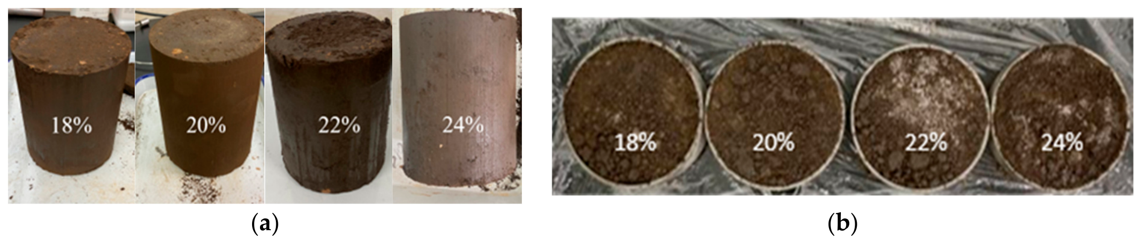
Standard specimens were prepared using ring cutters featuring a diameter of 61.8 mm and a height of 20 mm. Each experimental set consisted of four individual specimens. The specimens were wrapped in plastic film to minimize moisture loss. The testing environment was regulated by an environmental chamber. The apparatus maintained the temperatures at −5 °C, −10 °C, −15 °C, −20 °C, and −25 °C. Freezing treatment of the specimens was conducted under these defined conditions for a duration of 12 h. Figure 3 illustrates the appearance of the frozen soil specimens.

3.2. Dataset Composition and Feature Summary

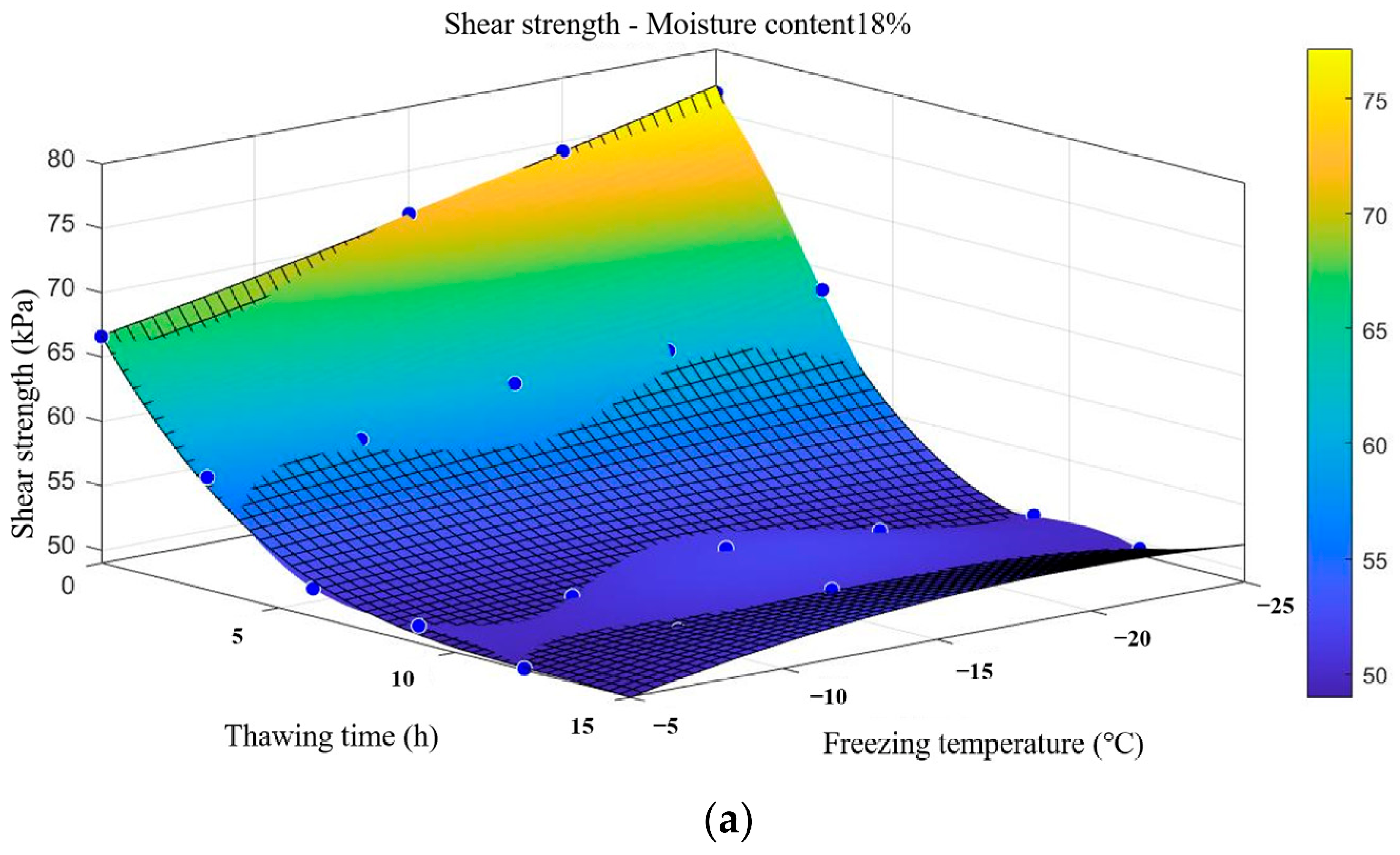
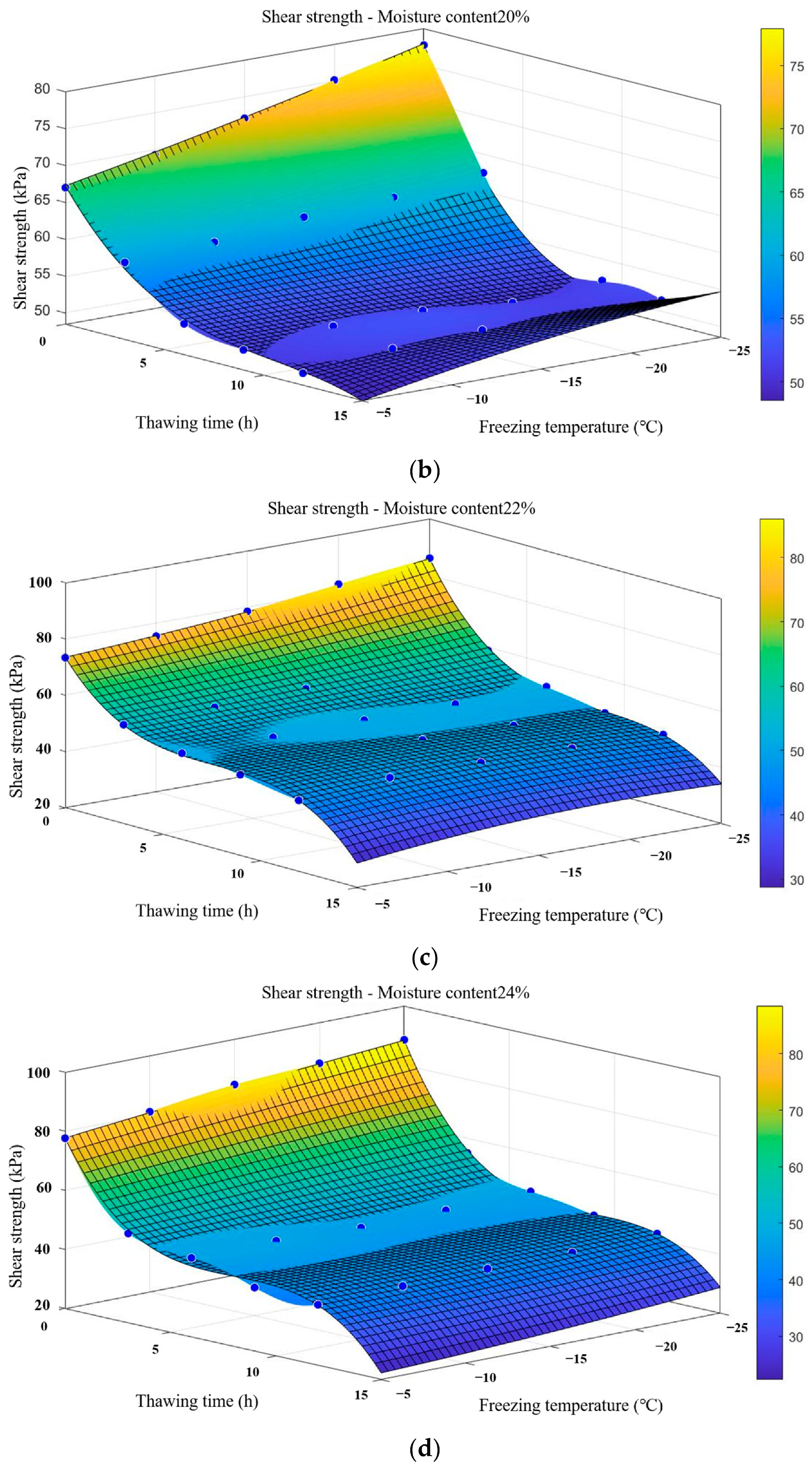
Measurements of soil shear strength were conducted using direct shear tests. A constant normal stress of 100 kPa was maintained throughout the procedure. The testing evaluated moisture contents of 18%, 20%, 22%, and 24%. Controlled temperatures used in the freezing treatment were −5 °C, −10 °C, −15 °C, −20 °C, and −25 °C. After the freezing stage, the samples were allowed to thaw at room temperature. Thawing durations of 0, 3, 6, 9, and 12 h were allocated to the experimental plan. Therefore, moisture content, freezing temperature, and thawing duration comprised four, five, and five distinct levels, respectively. This combination led to 100 independent data points. The experimental design incorporated 100 soil samples. The resulting shear strength values correspond to the moisture content values of 18%, 20%, 22%, and 24%. Experimental data points are shown as blue dots in Figure 3. These data points were fitted by a Gaussian Process Regression model to generate the response surface. Soil specimens with 18% moisture content demonstrate a specific strength response. The observed shear strength ranges from 49.12 kPa to 76.59 kPa. At 20% moisture content, the values range from 50.17 kPa to 77.73 kPa. The shear strength ranges from 45.31 kPa to 86.31 kPa in the case of 22% moisture content. Lastly, the shear strength of the specimens ranges from 40.56 kPa to 88.51 kPa when the moisture content is 24%.

4. Model Architecture and Implementation

4.1. Methodological Overview

The theoretical foundation of the proposed methodology is substantially corroborated by recent advancements documented in relevant geotechnical literature. Specifically, standard physics-informed neural networks have been successfully implemented by various researchers for solving complex geomechanical boundary value problems and predicting soil deformation [44]. Furthermore, self-supervised representation learning techniques have been increasingly utilized to extract underlying latent features from sparse geological datasets [45]. Built upon these prior studies, a unified framework integrating these two distinct paradigms is specifically introduced in this section to address the unique geomechanical challenges associated with seasonal frost degradation.
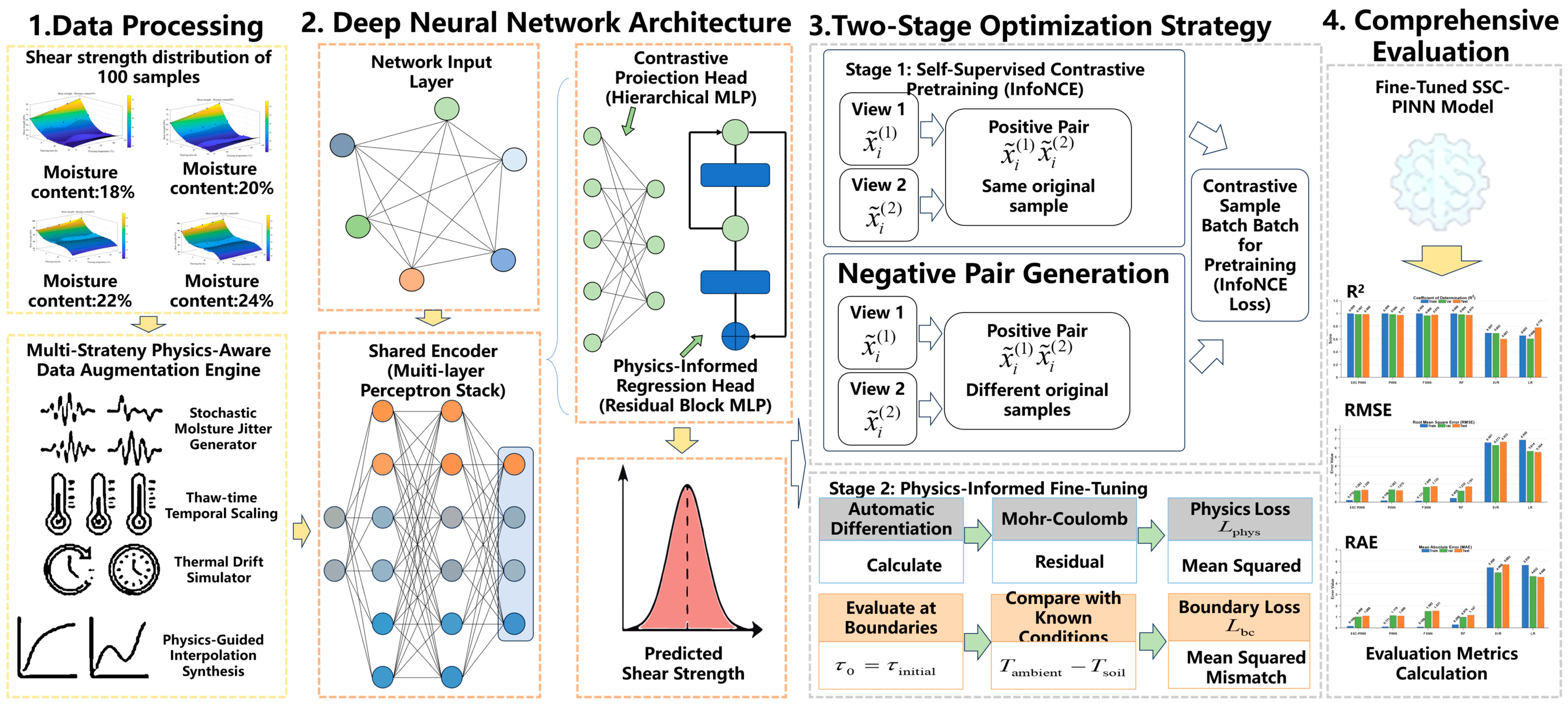
The overall structure of the proposed method is shown in Figure 4. The architecture is divided into four interrelated stages. The initial stage involves the process of data preprocessing. At this step, an analysis is performed to determine the shear strength distribution of the 100 samples. A multi-strategy physics-conscious data augmentation engine is utilized to enhance the training set. It employs several techniques to do so. The specific operations include stochastic moisture jitter and temporal scaling of thawing duration. Thermal drift simulation and physics-based interpolation are also incorporated.
The second phase comprises the deep neural network architecture. This component features a hierarchical design. The architecture consists of the network input layer and a shared encoder. The shared encoder utilizes a multi-layer perceptron stack. It also includes a contrastive projection head and a physics-informed regression head. Additionally, the regression head contains residual blocks to predict shear strength.
The third stage involves a two-stage optimization process. Self-supervised contrastive pretraining is executed as the first optimization step. An InfoNCE loss function is utilized to perform this operation. This loss enables the network to learn representations based on positive and negative sample pairs. Subsequently, the second optimization step executes physics-informed fine-tuning. Automatic differentiation is used to compute the required derivatives. The model is constrained by the Mohr–Coulomb constitutive residuals. Boundary condition penalties are also implemented at this stage.
The final stage involves an overall evaluation. Evaluation metrics are computed to assess the fine-tuned SSC-PINN model. This procedure verifies the predictive accuracy as well as physical consistency. The subsequent sections provide a detailed description of these components.

4.2. Neural Network Architecture Design

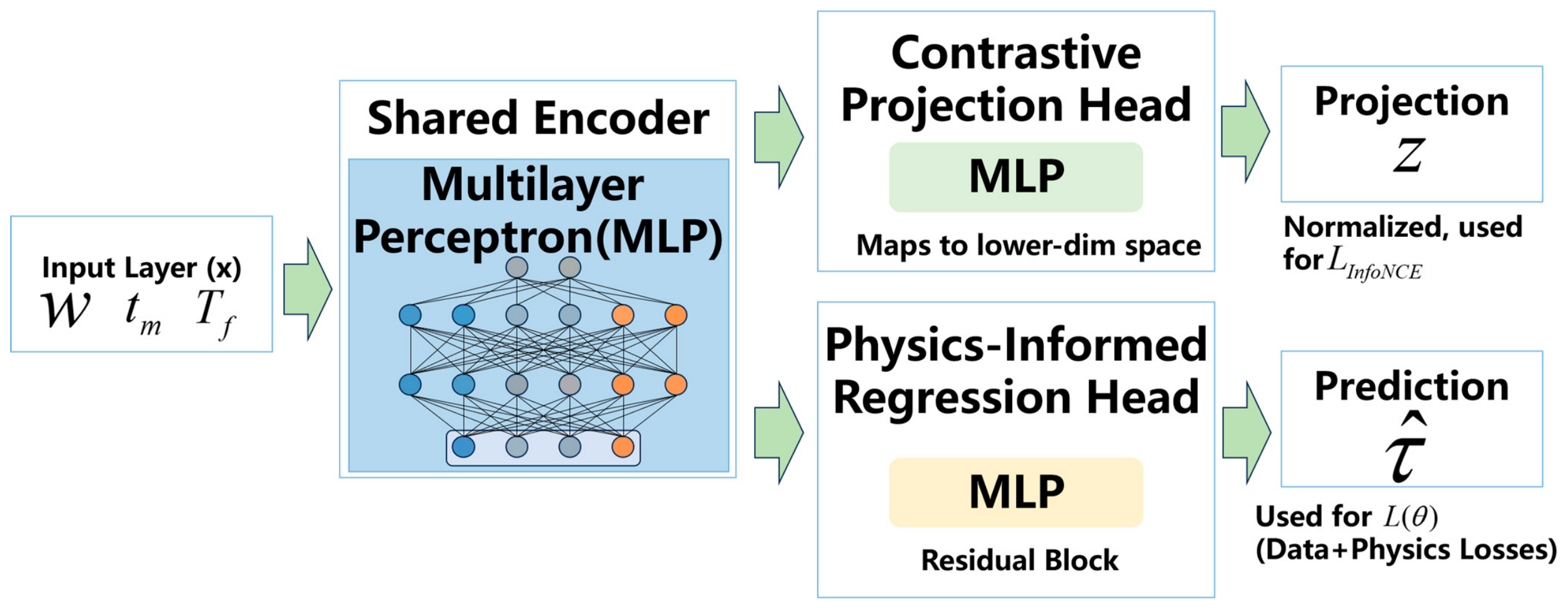
Figure 5 illustrates the architecture of the SSC-PINN framework. This network configuration comprises three interrelated modules that constitute the neural network. These components consist of a shared encoder and a contrastive projection head. The network also incorporates a physics-informed regression head. Each module operates under specific structural constraints. These design decisions balance the representational capacity and physical consistency of the model. Computational efficiency is also maintained through these structural configurations.
The shared encoder is a fully connected multilayer perceptron (MLP). To prevent overfitting on the limited empirical dataset of 100 samples, the network complexity was strictly constrained. Based on the rigorous structural sensitivity analysis detailed in Section 5.3, the optimal architecture was scaled down. Consequently, the shared encoder is configured with 3 hidden layers, each containing 64 neurons. Each hidden layer is followed by Gaussian Error Linear Unit (GELU) activations. These activations promote smooth gradient flow throughout the network. This smooth flow benefits both the contrastive and PINN loss components [46].
Layer normalization is applied prior to every activation function. This step stabilizes training regardless of data augmentation. It also regulates the residuals of the differential equations. Additionally, the network incorporates residual pre-activation connections. These connections link the first and third hidden layers. This design facilitates efficient information propagation and mitigates the vanishing gradient problem.
The contrastive projection head maps high-dimensional encoder features to a lower-dimensional space. The framework evaluates the InfoNCE loss within this target space. This mapping is executed by a two-layer MLP with layer dimensions of 128, 64, and 32. A ReLU activation follows the first layer, followed by batch normalization. The architecture L 2 -normalizes the final outputs. This constraint projects the outputs onto a unit hypersphere. Moreover, the projection head is separated from the regression head. This structural separation ensures component independence. Consequently, contrastive pretraining does not directly interfere with the physical prediction outputs.
The physics-informed regression head maps encoder features into shear strength predictions while incorporating physical constraints. It comprises three components: a feature expansion layer, a residual block, and an output layer. The feature expansion layer is a fully connected layer mapping 128 to 64 units with a tanh activation function to better capture nonlinear constitutive relations. The residual block has a two-layer bottleneck with GELU activations and a skip connection allowing a more complicated, physics-sensitive mapping. The last layer comprises a linear neuron which generates the end prediction. Physical integration is provided by using the regression head output to calculate the data-fitting loss and PDE residuals by applying the automatic differentiation of network outputs with respect to the input variables.

4.3. Incorporation of Physical Constraints: Constitutive Laws and Boundary Conditions

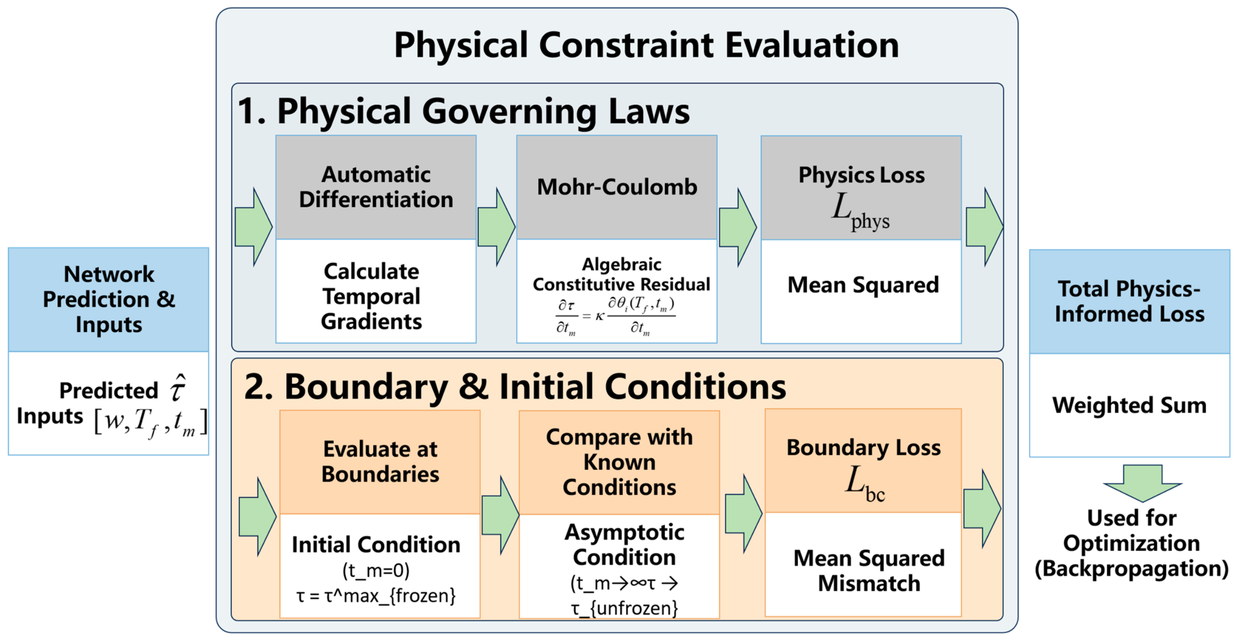
The SSC-PINN model enforces physical constraints to guarantee compliance with the underlying physical rules in addition to standard data fitting. These laws govern the mechanical reaction of seasonally frozen silty clay. The constraints are implemented directly in the loss function of the neural network in the framework. This mathematical formulation enforces consistency with the physical behavior of the soil system. The embedded physical principles include the constitutive laws of shear strength, the time-dependent governing differential equation, and corresponding boundary conditions. These components are depicted in Figure 6.
The problem addressed in this study is fundamentally a time-dependent constitutive modeling problem. It must be clarified that the classical Mohr-Coulomb criterion serves as an algebraic constitutive constraint rather than a spatial partial differential equation (PDE) [47]. The overall formulation of the algebraic constitutive law within the PINN is expressed as follows:
τ = c i c e ( T f , t m ) + σ tan ϕ ( w )
The components c i c e and ϕ are temperature and moisture-dependent. Specifically, the apparent cohesion c i c e provided by ice cementation degrades over the thawing duration t m . Instead of using undefined empirical functions, the temporal degradation of shear strength during the thawing process is mathematically constrained by a governing ordinary differential equation (ODE) with respect to thaw time t m :
τ t m = κ θ i ( T f , t m ) t m
Here, θ i represents the volumetric ice content, and κ is a physical coupling coefficient reflecting the sensitivity of cohesion to ice cementation degradation. The network utilizes automatic differentiation to compute the physical gradient τ t m of the predicted shear strength with respect to the input thaw time, ensuring that the empirical outputs strictly satisfy this temporal degradation rate.
Boundary conditions constitute the second type of physical constraint. The framework imposes appropriate constraints on the predicted shear strength to ensure consistency of physical properties throughout the experimental domain. Based on the geomechanical behavior of silty clay in seasonally frozen areas, a non-negativity constraint is imposed on the strength parameters [48]. Since the SSC-PINN models a time-dependent thawing process governed by [ w , T f , t m ] , the spatial thermal and moisture flux boundaries are replaced by rigorous temporal boundary conditions. The formulation takes into account the initial conditions before thawing and the asymptotic boundary conditions after complete thawing.
The pre-thawing state of initial soil moisture content and freezing temperature determines the maximum initial shear strength of the soil. This physical relationship is enforced within the model using boundary conditions specified at the initial time step ( t m = 0 ):
τ ( w , T f , t m = 0 ) = τ f r o z e n m a x ( w , T f )
Furthermore, an asymptotic boundary condition regulates the shear strength at the end of the freeze–thaw cycle. As the thawing duration t m extends to a sufficient period ( t m ), the volumetric ice content θ i 0 . At this thermodynamic boundary, the shear strength must degrade to a lower bound corresponding to the unfrozen state at that specific moisture content w . This constraint is explicitly prescribed as
lim t m τ ( w , T f , t m ) = τ u n f r o z e n ( w )
The network optimizes the boundary loss term L b c by computing the mean squared mismatch at these critical temporal boundaries, effectively penalizing predictions that violate the physical limitations of the fully frozen and fully thawed states.

4.4. Data Augmentation and Generation of Contrastive Sample Pairs

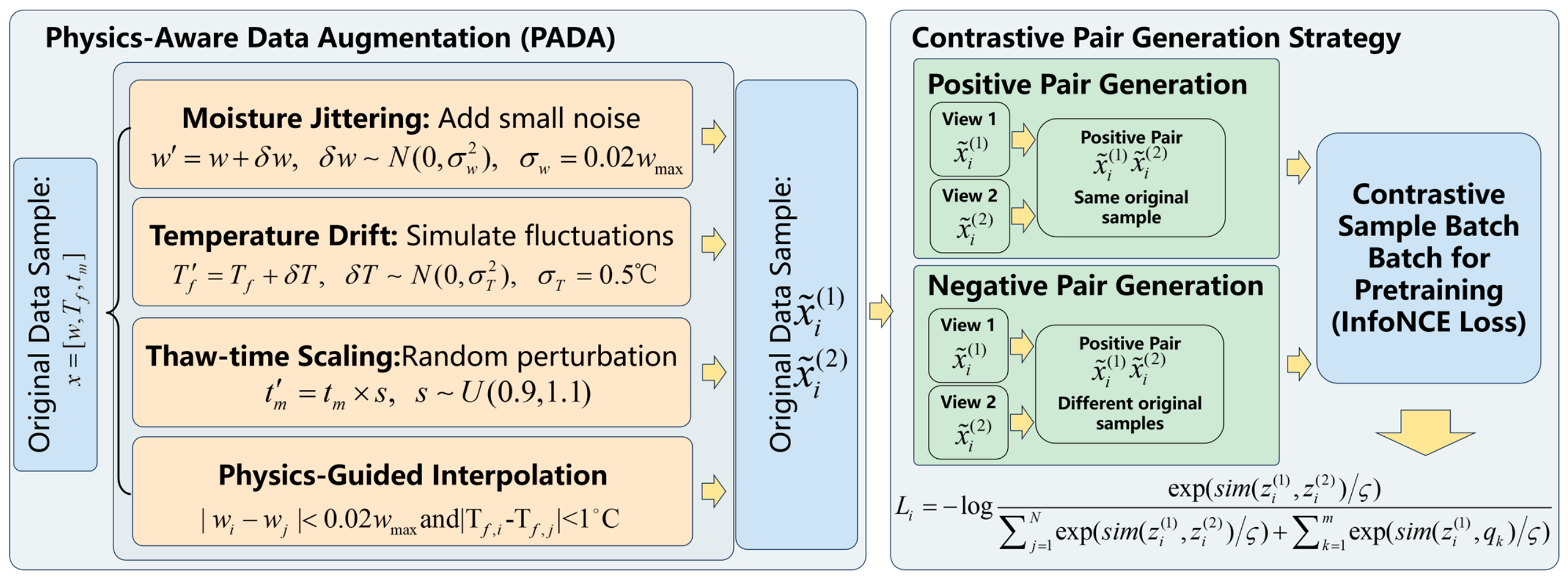
In order to alleviate data sparsity and enhance the resilience of the self-supervised contrastive learning step, a family of physics-informed augmentation operations are performed on every initial example. x = [ w , T f , t m ] (moisture content w , freezing temperature T f , thaw time t m ). Augmentations are designed to reflect realistic measurement noise and environmental variability, as shown in Figure 7.

4.4.1. Physics-Aware Data Augmentation

The lack of annotated shear strength data is alleviated by a group of data augmentation plans. The techniques rely on the physics of seasonally frozen silty clay. This domain-specific information allows these operations to enhance the generalization ability of self-supervised pretraining. These augmentations have three main goals. Firstly, simulation of laboratory measurement noise and environmental variables adds data variability without the need to conduct further lab experiments. Secondly, the framework achieves great physical stability. It is ensured that the added samples do not exceed realistic limits of moisture, temperature and time of thawing.
The physical limitations are imposed by laboratory guidelines and foundational soil mechanics. Consequently, the direct application of this specific augmentation methodology to other soil types is inherently restricted. The contrastive learning environment is optimized exclusively for the specific freeze thaw behavior and cohesive properties of silty clay. Therefore, the distinct geomechanical failure mechanisms observed in coarse granular soils or highly plastic clays might not be accurately represented by these specific minimal perturbations. A thorough recalibration of the physical boundaries is required before this framework is generalized to distinct geological materials. Nevertheless, within the investigated domain, the same latent shear strength characteristics are successfully retained by the produced views, and a robust contrastive learning environment is thereby created.
For each original sample x i , two independent augmentation pipelines produce views x ˜ i ( 1 ) and x ˜ i ( 2 ) . Augmentations reflect realistic measurement variability while preserving physical consistency:
(1)
Moisture jitter: Additive noise models sampling fluctuations:
w = w + δ w , δ w N ( 0 , σ w 2 ) , σ w = 0.02 w max
This simulates typical uncertainties in water-content measurement (±2%) [49].
(2)
Temperature drift: random perturbation within thermocouple accuracy:
T f = T f + δ T , δ T N ( 0 , σ T 2 ) , σ T = 0.5   ° C
Captures small inconsistencies in freezing-point control.
(3)
Thaw-time scaling: models environmental or procedural fluctuations in thaw duration:
t m = t m × s , s U ( 0.9 , 1.1 )
Ensures sample labels still reflect the same latent state within ±10% time variation.
(4)
Physics-Guided Interpolation: randomly select x j satisfying:
| w i w j | < 0.02 w max   and   | T f , i T f , j | < 1   ° C
Generate intermediate sample:
x = α x i + ( 1 α ) x j
Label via convex combination:
τ = α τ i + ( 1 α ) τ j
This method simulates continuous variations in freezing temperature and moisture content, leveraging linear combinations of soil responses. Through these procedures, the augmentation pipeline introduces physically meaningful variations into the training dataset. Consequently, during the contrastive learning phase, latent representations correlated with shear strength are explicitly captured. This optimization pathway prevents the network from overfitting to spurious noise artifacts. The framework implements these augmentations in an online manner, thereby maximizing computational efficiency and enhancing sample diversity during training.

4.4.2. Contrastive Pair Construction and Efficient Sampling

The augmentation step generates two distinct views for each given original sample. These views are subsequently integrated into the training pipeline via the pair generation module. This architectural design maximizes computational efficiency and enhances representational diversity during the training phase.
(1)
Dynamic Batch Formation
At each iteration, a minibatch of N unique samples is drawn, stratified to cover the full ranges of moisture content and freezing temperature. For each sample i the two augmented views x ˜ i ( 1 ) and x ˜ i ( 2 ) . are loaded, yielding a composite batch of size 2 N .
(2)
In-Batch View Arrangement
The batch tensor is organized so that indices [ 0 N 1 ] correspond to the first views and [ N 2 N 1 ] to the second views. This layout allows direct indexing of positive pairs [ i , i + N ] and efficient vectorized computation of cosine similarities for all pairs.
(3)
Negative Sampling Strategy
Negatives for an anchor view include all other views within the current 2N batch. Optionally, a momentum-updated queue of size M stores past epoch embeddings to expand the negative set without increasing batch size. A subset of m M embeddings is randomly sampled per iteration to maintain variability.
(4)
Embedding Projection and Normalization
Encoder f θ maps views to intermediate features h = f θ ( x ˜ )
(5)
InfoNCE Loss Computation
For anchor z i ( 1 ) and its positive z i ( 2 ) compute:
L i = log exp ( s i m ( z i ( 1 ) , z i ( 2 ) ) / ς ) j = 1 N exp ( s i m ( z i ( 1 ) , z i ( 2 ) ) / ς ) + k = 1 m exp ( s i m ( z i ( 1 ) , q k ) / ς )
Here, q k are queue embeddings when using the memory bank, and ς is the temperature hyperparameter.

4.5. Performance Metrics

Several standardized regression metrics are utilized to evaluate and compare the performance of the SSC-PINN model against baseline methods. These indicators provide quantitative assessments of predictive accuracy and generalization capability. Furthermore, these metrics are employed to evaluate physical consistency in predicting the shear strength of seasonally frozen silty clay. Specifically, the evaluation criteria encompass Root Mean Squared Error (RMSE), Mean Absolute Error (MAE), and the Coefficient of Determination R 2 .
RMSE commonly evaluates the performance of regression models. This metric measures the average magnitude of the error between predicted shear strength values and true observed values. Because the mathematical calculation squares the error components, RMSE exhibits high sensitivity to large outliers. Therefore, the metric heavily penalizes predictions that deviate significantly from experimental measurements. The mathematical formulation is expressed as follows:
RMSE = 1 N i = 1 N ( τ ^ i τ i ) 2
where τ ^ i is the predicted shear strength for the i -th sample, τ i is the true shear strength for the i -th sample, and N is the total number of samples in the test set.
Root Mean Squared Error (RMSE) is a standard metric for evaluating regression model performance. This metric reflects the average magnitude of the prediction error between the estimated shear strength and experimental measurements. Because the mathematical formulation involves squaring the error terms, RMSE is highly sensitive to large outliers. Consequently, this metric heavily penalizes predictions that significantly deviate from the experimental results. The mathematical formulation is expressed as:
MAE = 1 N i = 1 N | τ ^ i τ i |
R 2 is a measure of how well the model explains the variance in the observed data. It compares the variance of the model’s predictions to the variance of the actual data. R 2 values range from 0 to 1, where a value of 1 indicates perfect predictions, and a value of 0 indicates that the model explains no variance. It is calculated as:
R 2 = 1 i = 1 N ( τ ^ i τ i ) 2 i = 1 N ( τ i τ ¯ i ) 2
where τ ¯ i is the mean of the true shear strength values. A higher R 2 indicates that the model explains a higher proportion of the variance in the test data. An R 2 value closer to 1 indicates that the model performs well in predicting shear strength.
In addition to conventional regression metrics, the physical consistency of the model predictions is systematically assessed. It is verified by this analytical step that the predicted shear strength conforms strictly to the governing physical laws defining the geomechanical behavior of seasonally frozen silty clay [40]. Based on the established mathematical formulation, the physics residual loss is calculated as the specific deviation between the predicted shear strength and the theoretical values derived from the constitutive model. Furthermore, stricter adherence to the underlying physical constraints of soil behavior is quantitatively indicated by lower residual values, as demonstrated in recent physics-informed modeling studies [42].

4.6. Data Splitting Strategy and Baseline Models for Comparison

The experimental dataset consists of 100 independent samples used for training and evaluating the performance of the SSC-PINN model. The data encompasses a wide range of environmental variables. Specifically, the soil moisture content levels are 18%, 20%, 22%, and 24%. The freezing temperatures are −5 °C, −10 °C, −15 °C, −20 °C, and −25 °C. The thawing durations are 0 h, 3 h, 6 h, 9 h, and 12 h. The entire dataset is partitioned into three distinct subsets to ensure a rigorous evaluation of model generalization. Figure 8 shows the distribution of these 100 data points.
The training set comprises 70% of the overall data (70 samples). This specific partitioning ratio of 70%, 15%, and 15% is widely recognized as an optimal configuration in computational geomechanics to provide sufficient training data while preventing overfitting [44]. Both self-supervised contrastive pretraining and physics-informed fine tuning utilize this subset. During the training phase, online data augmentation generates multiple views of each sample, enabling the network to acquire noise invariant feature representations. The validation set comprises 15% of the data (15 samples). This subset is used to monitor training convergence and optimize hyperparameters. Early stopping procedures are also implemented in the workflow to mitigate overfitting, thereby ensuring stable optimization. Finally, the remaining 15% of the data serves as the test set. This set contains 15 samples designated for impartial performance evaluation. This subset is completely excluded from the training and validation phases. This independent dataset evaluates the predictive ability of the model to extrapolate to unseen conditions.
Five baseline models are implemented to evaluate the effectiveness of the proposed SSC-PINN framework. These methods represent established techniques for predicting soil shear strength, incorporating varying degrees of physical principles integrated with data-driven mechanisms.
Linear Regression (LR) serves as the most fundamental baseline model. Linear models exhibit fundamental limitations in capturing the complex, highly nonlinear relationships inherent in geomechanical data. Nevertheless, it establishes a baseline performance floor, highlighting the advantages of sophisticated architectural configurations like SSC-PINN.
Support Vector Regression (SVR) is a widely adopted machine learning algorithm. It is extensively utilized for its capability to handle nonlinear mappings in regression through kernel functions [50]. Optimized using the identical set of input features, this model serves as a benchmark for conventional data-driven approaches.
Random Forest Regression (RF) is a non-parametric ensemble learning method suitable for multidimensional regression tasks. Trained on the same input variables—specifically moisture content, freezing temperature, and thawing duration—and evaluated on the identical test split, RF provides a direct comparison to the proposed framework.
The Fully Supervised Neural Network (FSNN) baseline is optimized purely under data-driven supervision, excluding any physical or structural constraints. While FSNN shares the identical network architecture and feature space as SSC-PINN, it lacks the contrastive pretraining phase and physics-informed loss regularization. This comparison isolates the joint effects of self-supervised learning and physical constraints on the overall predictive accuracy.
The standard Physics-Informed Neural Network (PINN) incorporates physics-based loss terms to enforce the governing constitutive laws during optimization. However, it omits the self-supervised contrastive pretraining stage. Maintaining identical hyperparameter configurations and data splits as SSC-PINN, this baseline isolates and quantifies the specific impact of contrastive representation learning under identical physical constraints.

4.7. Training Procedure, Optimization Algorithm, and Hyperparameter Settings

The computational implementation of the proposed SSC-PINN framework was executed using MATLAB R2021b in conjunction with the Deep Learning Toolbox. Unlike traditional numerical analysis methods such as finite difference or finite element schemes, the temporal gradients required for the physical differential equations were computed exactly using the automatic differentiation capabilities inherent to MATLAB. Specifically, this was achieved through the implementation of dlarray objects and the dlgradient function, which evaluate derivatives at collocation points analytically, thereby eliminating truncation errors associated with numerical discretization. The optimization of the network parameters and the minimization of the composite loss function were driven by the Adam algorithm. All training and validation procedures were conducted on a workstation equipped with a dedicated graphics processing unit to accelerate matrix computations.
The optimization of the SSC-PINN framework is executed through a two-stage sequential implementation. The procedure initiates with self-supervised contrastive pretraining and concludes with physics-informed fine-tuning. In the first stage, self-supervised contrastive learning utilizes augmented representations of the input dataset. An augmentation pipeline generates dual augmented views for each discrete sample through methods including Gaussian jitter, thermal drift simulation, and thaw-time temporal scaling. The training minimizes a contrastive loss function to maximize the embedding similarity between correlated augmented views (positive pairs). Concurrently, the loss segregates the representations of distinct samples (negative pairs). This pretraining strategy enables the encoder to extract robust, noise-resistant feature representations prior to downstream task adaptation. The pretraining phase typically terminates after 50 to 100 epochs upon convergence of the contrastive loss.
The subsequent fine-tuning stage incorporates physical regularizers into the model. The objective function integrates the contrastive loss with a physics-informed loss term to enforce strict physical consistency. The physics-informed loss encompasses domain-specific constraints, including the governing constitutive equations of shear strength and the boundary conditions of the geotechnical system. This joint optimization scheme ensures high fidelity to empirical data while maintaining strict adherence to the underlying physical laws of seasonally frozen silty clay. Fine-tuning proceeds until both objective components are simultaneously minimized, thereby optimizing both predictive accuracy and physical validity.
The Adam optimizer is employed within the training pipeline to update the network parameters. This algorithm is well suited for the high dimensional parameter spaces and sparse gradient fields typical of physics-informed architectures, as demonstrated by recent advanced computational studies [42]. It dynamically adjusts individual learning rates based on the first and second moments of the gradients. The initial learning rate is set to 10 3 . A step decay scheduler reduces the learning rate by half every 20 epochs. This learning rate attenuation facilitates stable convergence during the fine tuning phase. Furthermore, highly nonlinear differential terms can induce gradient explosion; to mitigate this, gradient clipping with a maximum norm constraint of 5.0 is enforced during physics-informed training [51].
Hyperparameter calibration establishes an optimal balance among predictive accuracy, generalization capacity, and computational efficiency within the SSC-PINN framework. The batch size is set to 32 to stabilize gradient estimation and optimize memory utilization. The contrastive temperature parameter τ is set to 0.1 to regulate the scaling of similarity penalties between positive and negative pairs in the loss function. To mitigate overfitting, dropout regularization is incorporated; specifically, a dropout rate of 0.1 is applied within the residual blocks of the regression head. A weight decay of 10 5 is applied to all trainable parameters to constrain model complexity. Finally, an early stopping protocol with a patience of 20 epochs terminates the optimization if the validation loss fails to decrease, ensuring robust generalization to unseen data.
A critical aspect of optimizing the SSC-PINN framework is the calibration of the loss weighting coefficients ( λ data , λ phys and λ bc ) defined in Equation (3). The rationale for setting these weights is based on balancing the gradient magnitudes of the constituent loss terms to prevent any single constraint from dominating the optimization trajectory. Through systematic grid search evaluated on the validation dataset and monitoring of the gradient scales, the data fidelity weight ( λ data ) was anchored at 1.0 as the baseline. The physical residual weight ( λ phys ) and the boundary condition weight ( λ bc ) were empirically set to 0.5 and 0.5, respectively [52]. This configuration mathematically ensures that the network prioritizes fitting the observed shear strength while providing sufficient penalty gradients to enforce physical consistency and boundary compliance.
Despite the demonstrated predictive capabilities, specific theoretical and practical limitations associated with the proposed methodology must be explicitly acknowledged. Theoretically, the predictive accuracy of the model is inherently constrained by the fundamental assumptions of the incorporated physical equations; thus, highly complex multiphysics couplings not represented in the governing loss functions may not be perfectly captured. Practically, significant computational resources are demanded by the dual training phases, particularly during the contrastive optimization stage. Furthermore, the convergence stability is highly sensitive to hyperparameter configurations, necessitating extensive computational tuning procedures to achieve the optimal network architecture.

5. Results

5.1. Predictive Performance Comparison

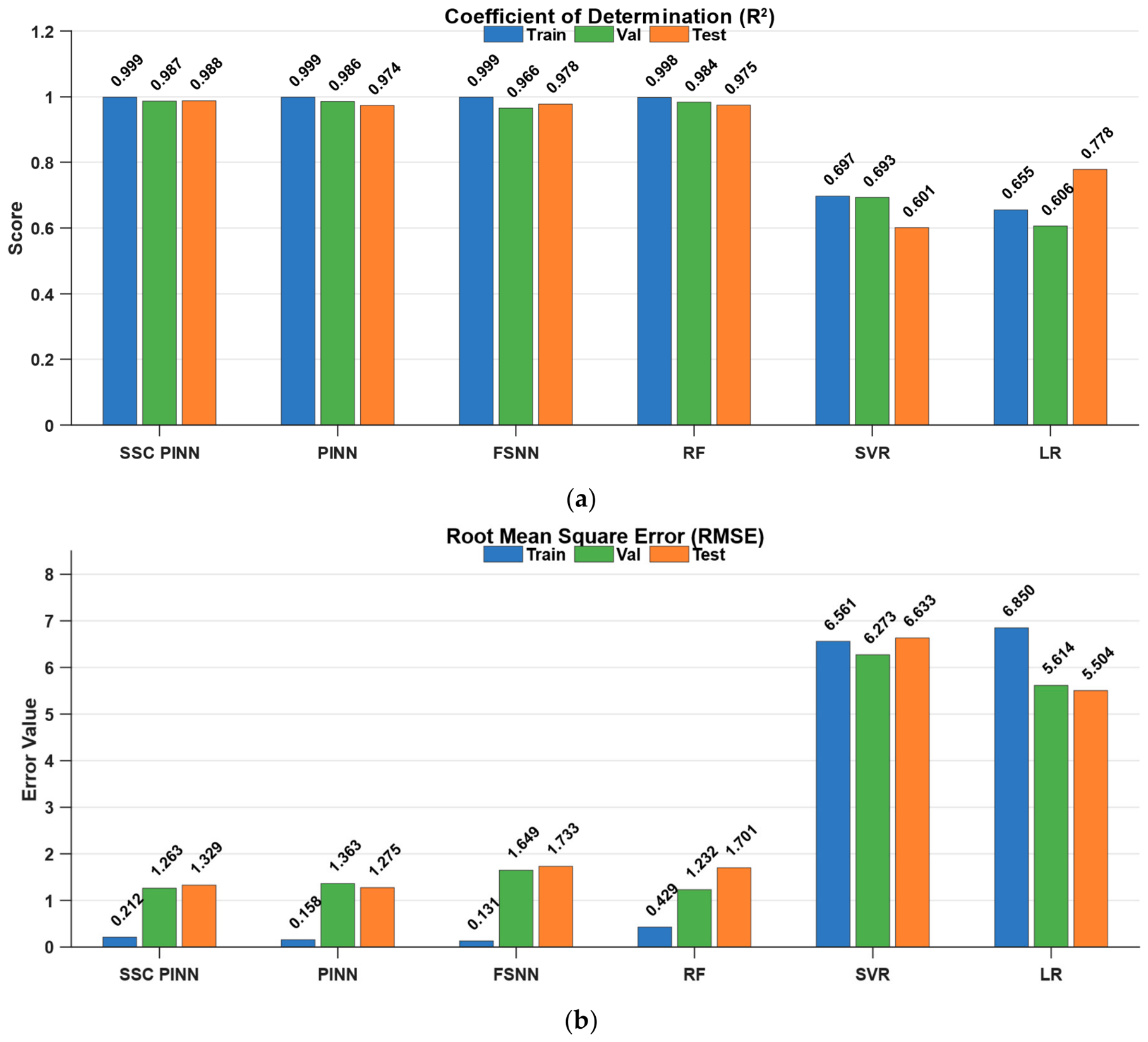
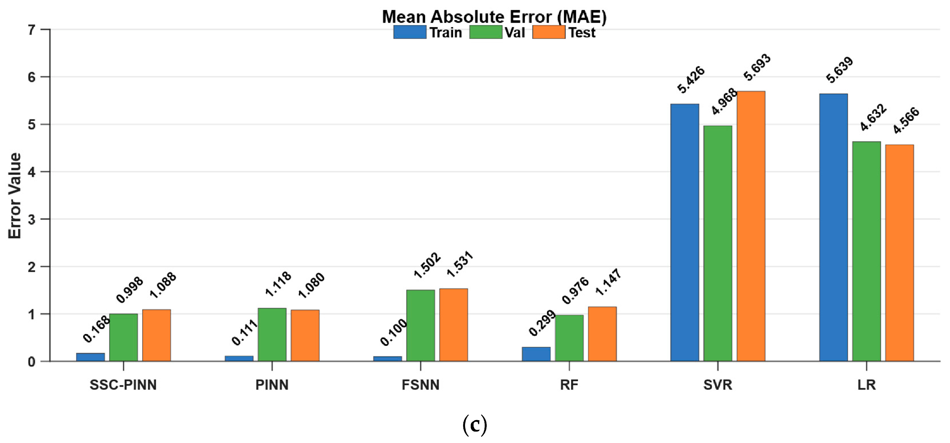
This section presents a systematic evaluation of the predictive performance of the proposed SSC-PINN framework relative to various baseline models. This comparison confirms the effectiveness of the framework in estimating the shear strength of seasonally frozen silty clay. The comparative baseline suite encompasses traditional machine learning algorithms as well as deep neural network architectures. Standard evaluation metrics, specifically the Coefficient of Determination ( R 2 ), Root Mean Squared Error (RMSE), and Mean Absolute Error (MAE), provide quantitative measures of model performance. Table 2 summarizes the statistical outcomes and performance comparisons, while Figure 9 illustrates these evaluation results.
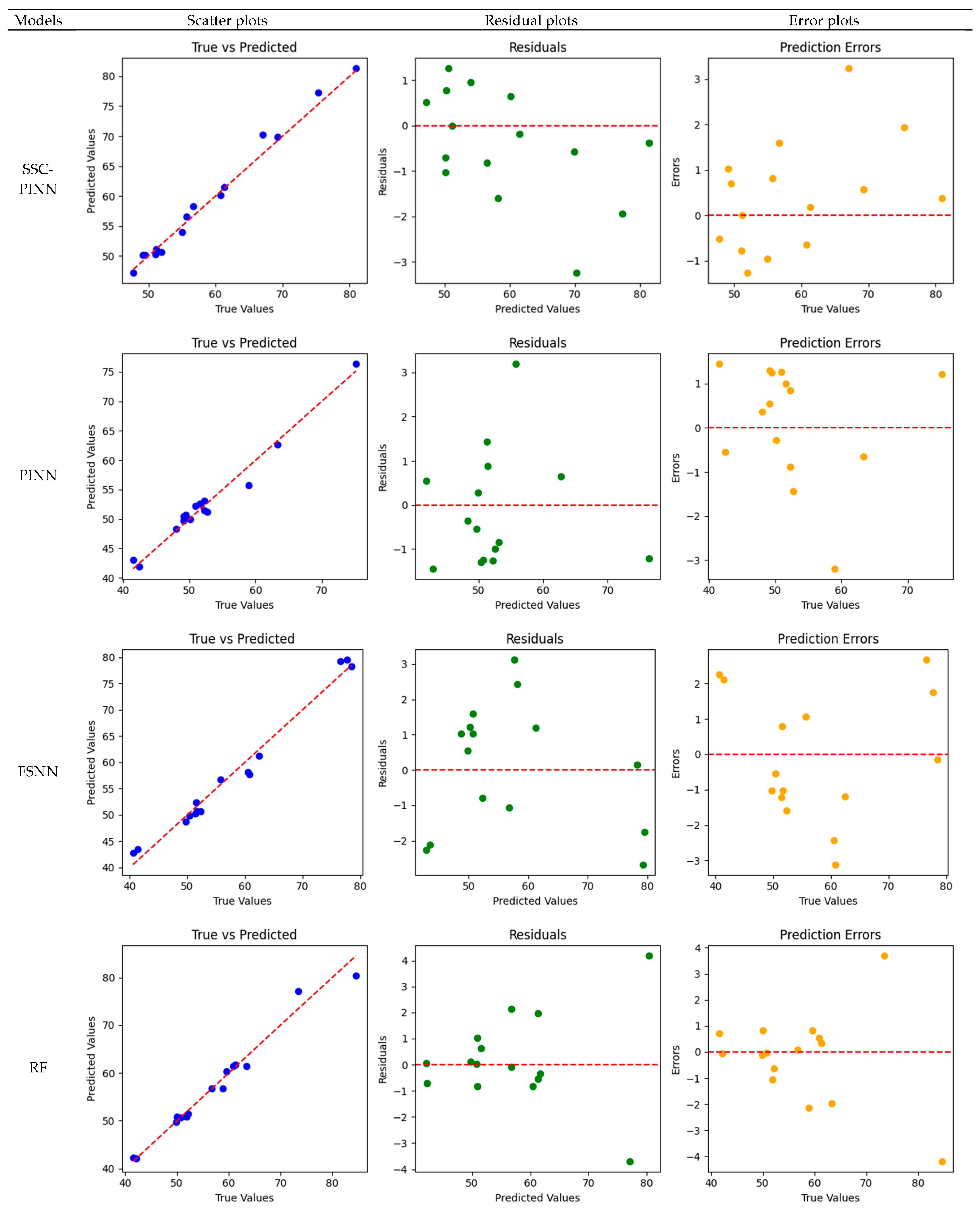
The performance comparison indicates that the proposed SSC-PINN framework outperforms all baseline models across all primary evaluation metrics. Specifically, the framework achieves the highest coefficient of determination ( R 2 = 0.988 ) on the test set. The model also yields the lowest RMSE (1.329) and MAE (1.088), demonstrating high predictive accuracy and generalization capacity. The standard PINN, which incorporates physics-informed constraints without the contrastive learning stage, exhibits competitive performance with an R 2 of 0.974; nonetheless, both its RMSE and MAE values are higher than those of the SSC-PINN. The FSNN provides acceptable forecasts with an R 2 of 0.978, yet it is outperformed by the SSC-PINN due to the latter’s lower error metrics. Conventional machine learning techniques exhibit lower accuracy; specifically, RF and SVR yield R 2 values of 0.975 and 0.601, respectively, while the LR model produces significant prediction errors with an R 2 of 0.778. These findings demonstrate the efficacy of integrating self-supervised contrastive learning with a physics-informed loss formulation. This combination significantly enhances geomechanical modeling performance, offering distinct advantages for characterizing the shear strength of seasonally frozen silty clay.
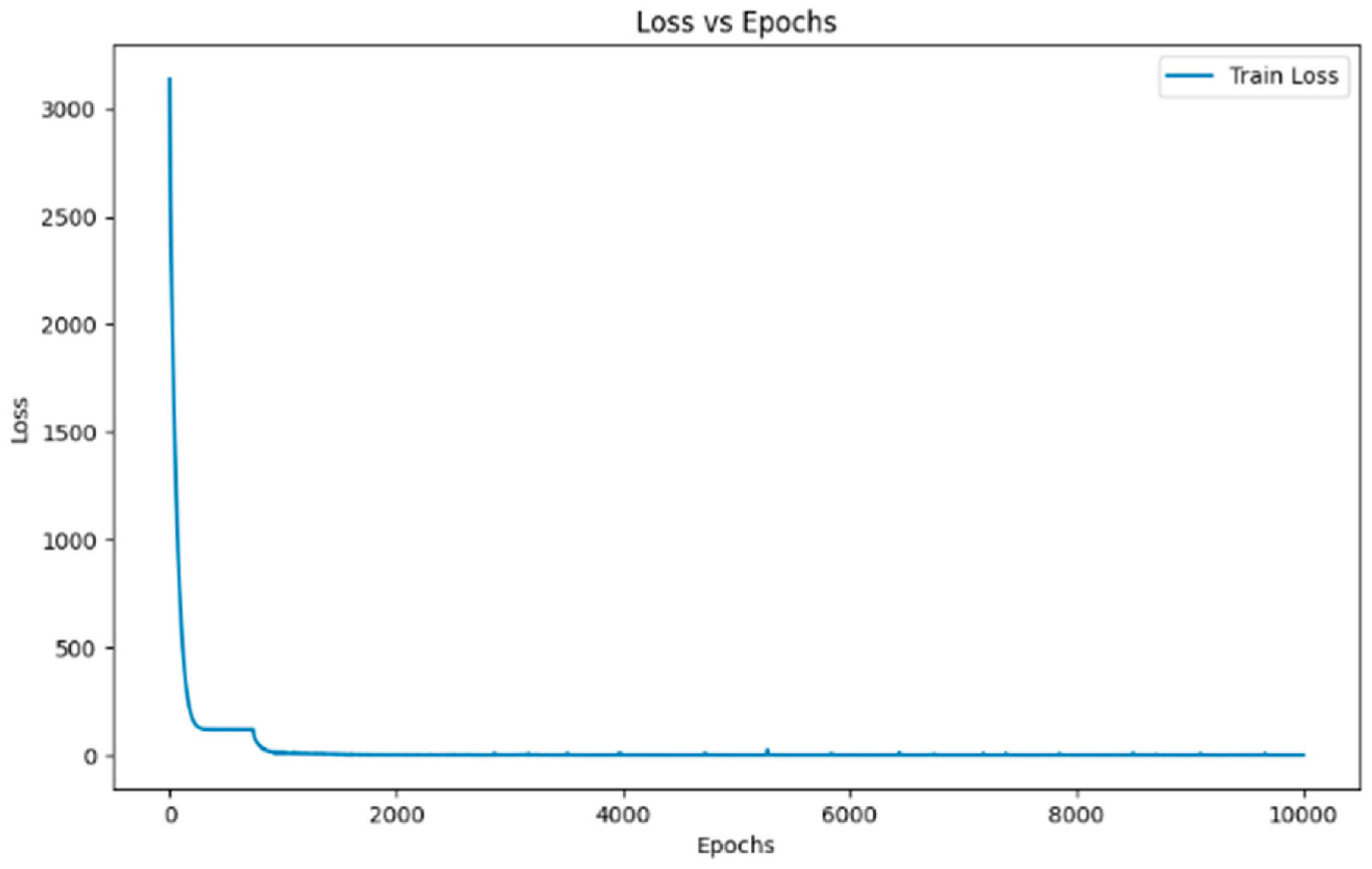
Figure 10 illustrates the convergence path of the objective function for the SSC-PINN model. The curve exhibits an optimization pattern characteristic of deep neural network architectures. This behavior features a sharp decrease in the total loss during the initial training epochs, followed by an asymptotic stabilization phase. Within this phase, minor statistical fluctuations are observed. At the onset of optimization, the network rapidly adjusts its parameter space to capture the primary features and multidimensional correlations inherent in the dataset. This rapid adjustment demonstrates its capability to efficiently reduce empirical error.
In the later stages of training, the loss curve stabilizes, indicating that the model has approached an optimal state within the solution space. Marginal oscillations occur during this period, reflecting localized adjustments in network weights. These adjustments yield incremental refinements to the predictive response surface. The convergence of the objective function to a well-defined minimum validates the efficacy of the optimization framework. The process effectively minimizes both the empirical data-driven loss and the physics-informed residual components. Consequently, the network achieves high predictive accuracy while strictly satisfying the prescribed boundary conditions and constitutive laws. This training behavior confirms the robustness of the structural configuration of the SSC-PINN framework. The optimization pathway ensures that the learned latent representations correlate strongly with the underlying physical laws governing seasonally frozen soil mechanics.
Figure 11 illustrates the scatter plots, residual distributions, and error profiles of the six comparative models. The performance comparison indicates that the SSC-PINN framework exhibits the highest predictive accuracy. Specifically, the model achieves a test coefficient of determination ( R 2 ) of 0.988. The optimization also yields the lowest RMSE and MAE values of 1.329 and 1.088, respectively. The SSC-PINN framework demonstrates superior generalization capability compared to the standard PINN and FSNN architectures, which is achieved by effectively coupling self-supervised contrastive representation learning with domain-specific physical constraints. Conversely, conventional data-driven methods—specifically Random Forest (RF), Support Vector Regression (SVR), and Linear Regression (LR)—are significantly less precise. Their lower accuracy highlights the inherent limitations of these methods in capturing the nonlinear geomechanical behavior of the soil matrix. These findings validate the efficacy of the unified SSC-PINN framework, demonstrating that the integration of self-supervised representation learning with physics-informed loss formulations substantially enhances both model robustness and predictive reliability.

5.2. Ablation Study

An ablation study is conducted to evaluate the relative contributions of the primary architectural components within the proposed SSC-PINN framework. This analysis assesses the specific functions of key components, namely self-supervised contrastive learning and physics-informed loss regularization, measuring their direct effects on overall predictive accuracy and generalization performance. Table 3 summarizes the statistical metrics for each ablation configuration, including the Coefficient of Determination R 2 , Root Mean Squared Error (RMSE), and Mean Absolute Error (MAE), with comparisons illustrated in Figure 12.
The ablation analysis demonstrates the critical roles of both self-supervised contrastive learning and physics-informed loss regularization in defining the complete SSC-PINN framework. The full SSC-PINN model, which integrates both components, achieves superior performance across all evaluation metrics. Specifically, it yields a test R 2 of 0.988, an RMSE of 1.329, and an MAE of 1.088. These quantitative results indicate that coupling contrastive learning with physics-informed loss functions provides highly accurate and robust predictions of soil shear strength, where the contrastive module enhances latent representations while the physics-informed loss enforces physical consistency.
Eliminating either architectural element results in a significant deterioration in predictive accuracy. The standard PINN structure, which incorporates the physics-informed loss but lacks contrastive learning, achieves a test coefficient of determination R 2 of 0.974 and a test RMSE of 1.275. This indicates that while physics-informed regularization provides critical optimization guidance, this variant underperforms compared to the full SSC-PINN architecture. Conversely, the ablation variant utilizing only self-supervised contrastive learning displays a substantial reduction in accuracy due to the omission of physics-informed loss terms. This variant yields a test R 2 of 0.860, an RMSE of 2.350, and an MAE of 2.200. This performance degradation highlights the consequences of neglecting physical constraints; although contrastive learning enhances latent feature extraction, omitting physical laws compromises generalization capability, causing predictions to deviate from the actual mechanical behavior of frozen soils.
The FSNN baseline, which lacks both self-supervised pretraining and physics-informed regularization, provides a test R 2 of 0.978. Nevertheless, the unified SSC-PINN framework ultimately outperforms this baseline. These comparative results demonstrate the efficacy of the proposed architectural modifications. Systematically introducing either data-driven representation learning or domain-specific physical constraints enhances both the predictive performance and generalization capability of the network. In conclusion, the ablation experiment highlights the paramount role of integrating data-driven representation learning with physical domain knowledge in geomechanical predictive modeling. The assessment demonstrates that the proposed SSC-PINN framework serves as an effective methodology for predicting the shear strength of seasonally frozen silty clay, yielding significant advancements over conventional machine learning algorithms and purely supervised neural networks.
Furthermore, to provide a comprehensive context regarding other research methodologies, these internal ablation outcomes are explicitly cross referenced with the comparative analysis detailed in Section 5.1. As demonstrated in that section, the unified SSC PINN framework not only surpasses its own architectural variants but also significantly outperforms established models such as Random Forest and Support Vector Regression, which are frequently utilized in contemporary geotechnical research. Therefore, it is firmly demonstrated by this integrated assessment that the proposed framework yields significant advancements over both purely supervised neural networks and conventional machine learning algorithms.

5.3. Sensitivity Analysis of Key Hyperparameters

This section presents a systematic sensitivity analysis to evaluate the effects of core hyperparameters on the predictive performance and optimization stability of the SSC-PINN model. Hyperparameter calibration ensures optimal convergence and enhances generalization capacity to unseen data. By varying these parameters within designated intervals, the distinct contributions of each hyperparameter to predictive accuracy and structural stability can be quantitatively determined.
The sensitivity evaluation targets key architectural and optimization hyperparameters. First, the learning rate η regulates the step size during gradient backpropagation; an excessively high learning rate can cause the optimization pathway to oscillate or overshoot the optimal solution, whereas an overly low rate leads to slow convergence or entrapment in local minima [42]. The evaluated range for the learning rate is { 10 4 , 10 3 , 10 2 , 10 1 } . Second, the number of hidden layers defines the network depth, which determines the structural capacity of the model. The capability of the network to map complex nonlinear geomechanical relationships is significantly enhanced by increasing the hidden layer count. However, the risk of overfitting is inevitably increased by an excessively deep architecture, especially when small sample sizes are utilized [53]. This hyperparameter is tested within the range of { 2 , 3 , 4 , 5 } . Third, the network width is controlled by the number of neurons per hidden layer, and the representation capacity of the model is thereby dictated. Intricate soil behavior patterns can be successfully captured when the network width is expanded. However, severe overparameterization can be induced by excessively large configurations, and overfitting is consequently caused, as documented in established deep learning literature [53]. The prescribed evaluation range is { 32 , 64 , 128 , 256 } .
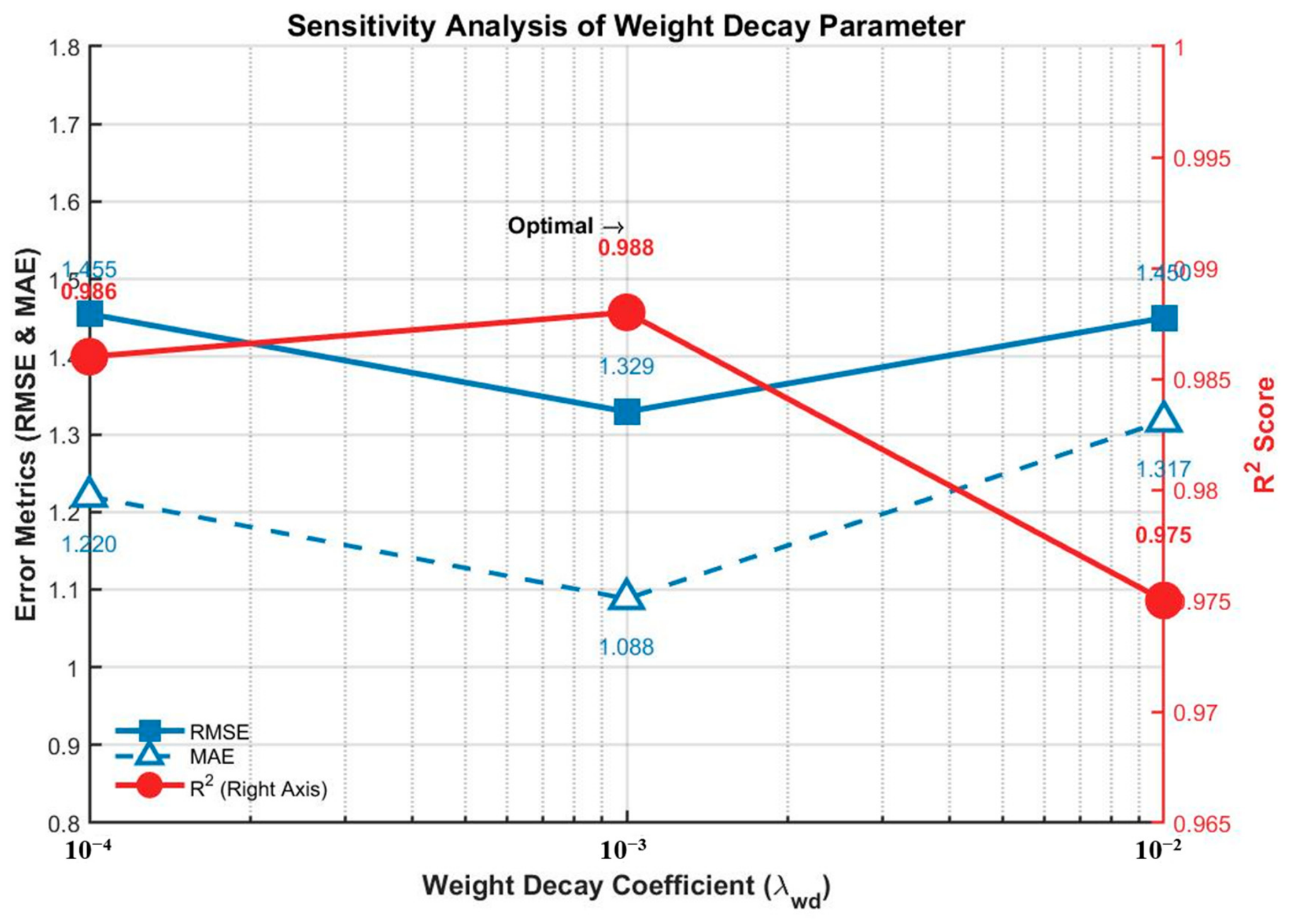
The remaining parameters govern the optimization dynamics and regularization constraints of the framework. Fourth, the batch size defines the number of training samples processed per forward and backward pass. Stochastic gradient noise is introduced by smaller batch sizes, and the model is theoretically assisted in escaping saddle points by this noise, although convergence may be destabilized. Conversely, consistent gradient estimates are yielded by larger batch sizes at higher computational costs, as extensively documented in neural network optimization literature [54]. The selected evaluation range is { 16 , 32 , 64 } . Fifth, weight decay is implemented as an L 2 regularization penalty to mitigate overfitting by penalizing excessive parameter magnitudes. While model complexity is effectively restricted by stronger regularization, network expressiveness is severely dampened by overly high penalties, and the effective representation of underlying physical laws is thereby prevented, as established in fundamental machine learning literature [55]. The evaluated range is { 10 2 , 10 3 , 10 4 } . Sixth, the sharpness of the similarity distribution between positive and negative sample pairs within the contrastive objective function is regulated by the contrastive temperature parameter. A smoother probability distribution is yielded by a higher temperature, whereas the distribution is sharpened by a lower temperature, thereby forcing the optimization to focus on hard negative pairs, as extensively detailed in contrastive learning literature [56]. The selected evaluation range is { 0.1 , 0.2 , 0.5 , 1.0 } .
To execute the sensitivity analysis, the SSC-PINN model is trained independently for 10,000 epochs under each specific hyperparameter configuration to ensure thorough optimization. Subsequently, the predictive performance on the test set is quantitatively evaluated using the previously defined statistical metrics. Specifically, the Coefficient of Determination ( R 2 ), Root Mean Squared Error (RMSE), and Mean Absolute Error (MAE) are computed to assess the accuracy, stability, and generalization capability of each model variant under identical validation conditions.
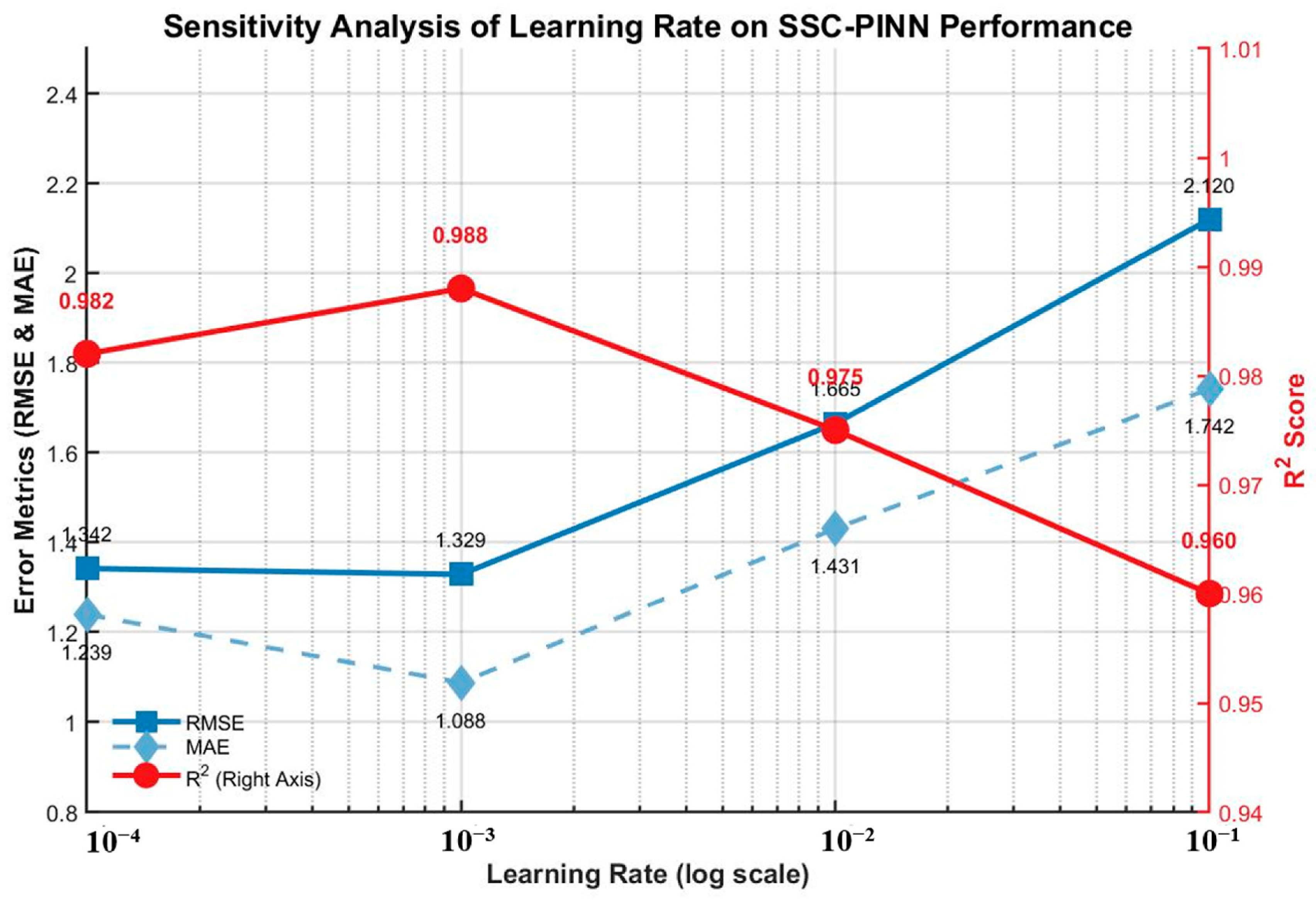
Table 4 presents a summary of the sensitivity analysis for the learning rate parameter ( η ), with the corresponding results illustrated in Figure 13. The evaluation indicates that the optimal learning rate is 10 3 , under which the model achieves a peak coefficient of determination ( R 2 ) of 0.988 and minimizes both RMSE and MAE values. Conversely, a smaller learning rate ( 10 4 ) results in insufficient optimization dynamics, leading to inadequate convergence within the prescribed training cycles. Excessively high learning rates ( 10 1 ) induce numerical instability, causing severe gradient oscillations and a drastic deterioration in predictive accuracy.
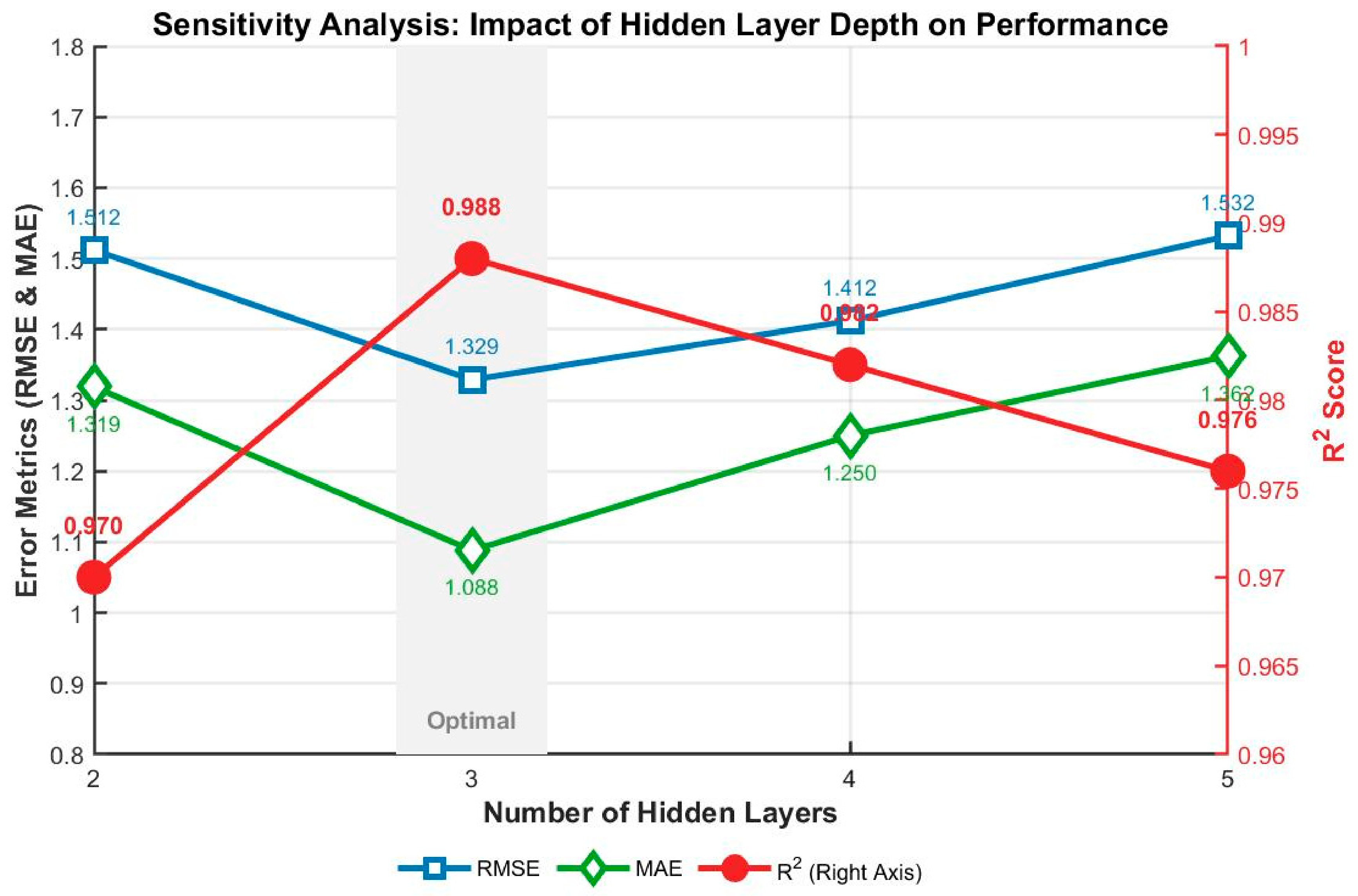
Table 5 summarizes the sensitivity analysis regarding the number of hidden layers, which defines the network depth, with the evaluation findings illustrated in Figure 14. The experimental results demonstrate that a three-layer configuration yields the optimal performance, achieving the maximum coefficient of determination ( R 2 ) while minimizing the RMSE and MAE values. Increasing the network depth beyond this optimal point results in diminishing returns or induces overfitting, as excessive parameter complexity weakens the generalization capacity of the model on the unseen test split.
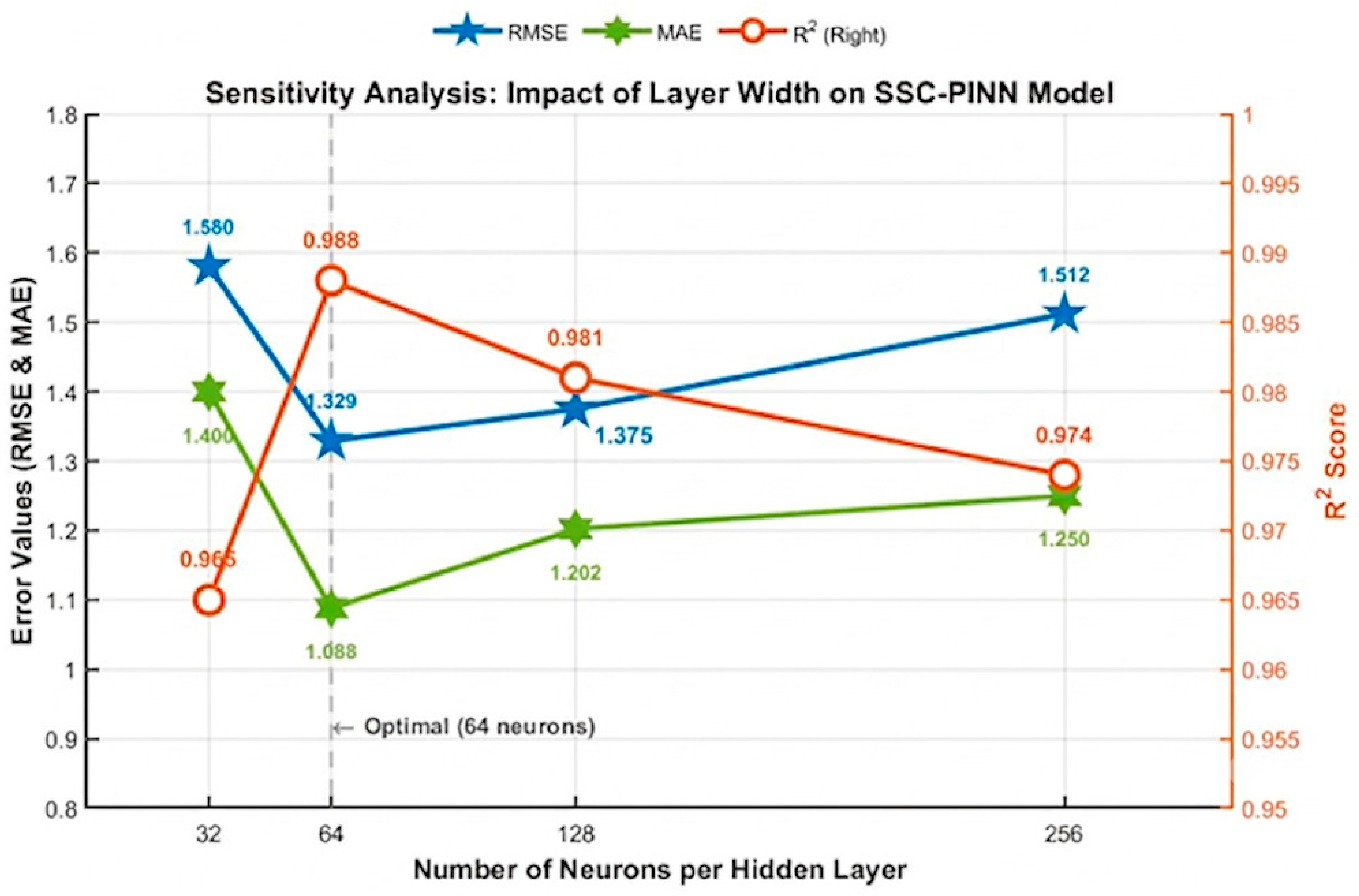
Table 6 presents the sensitivity analysis for the number of neurons per hidden layer, representing the network width, with the evaluation results depicted in Figure 15. The experimental findings indicate that optimal predictive performance is achieved with a configuration of 64 neurons per hidden layer. This setup establishes an effective balance between representational capacity and over-parameterization mitigation. A low neuron density (32 neurons) constrains the expressive capability of the network, restricting its ability to capture complex, multidimensional geomechanical interactions. Conversely, expanding the hidden layer width to 256 neurons yields diminishing returns; under this configuration, computational complexity increases and the risk of over-parameterization rises without producing a significant improvement in predictive accuracy.
This scaling-down analysis specifically verifies that the optimization trajectory does not get trapped in local minima and that the network does not overfit the 100 empirical data points. By constraining the architecture to 3 layers with 64 neurons, the degrees of freedom are appropriately balanced against the dataset size. Furthermore, it should be noted that the effective training size is significantly expanded beyond the 100 base samples. The self-supervised contrastive learning stage generates thousands of augmented views, and the physics-informed loss utilizes continuous collocation points across the temporal domain, providing massive structural regularization to guide the model toward the global optimum.
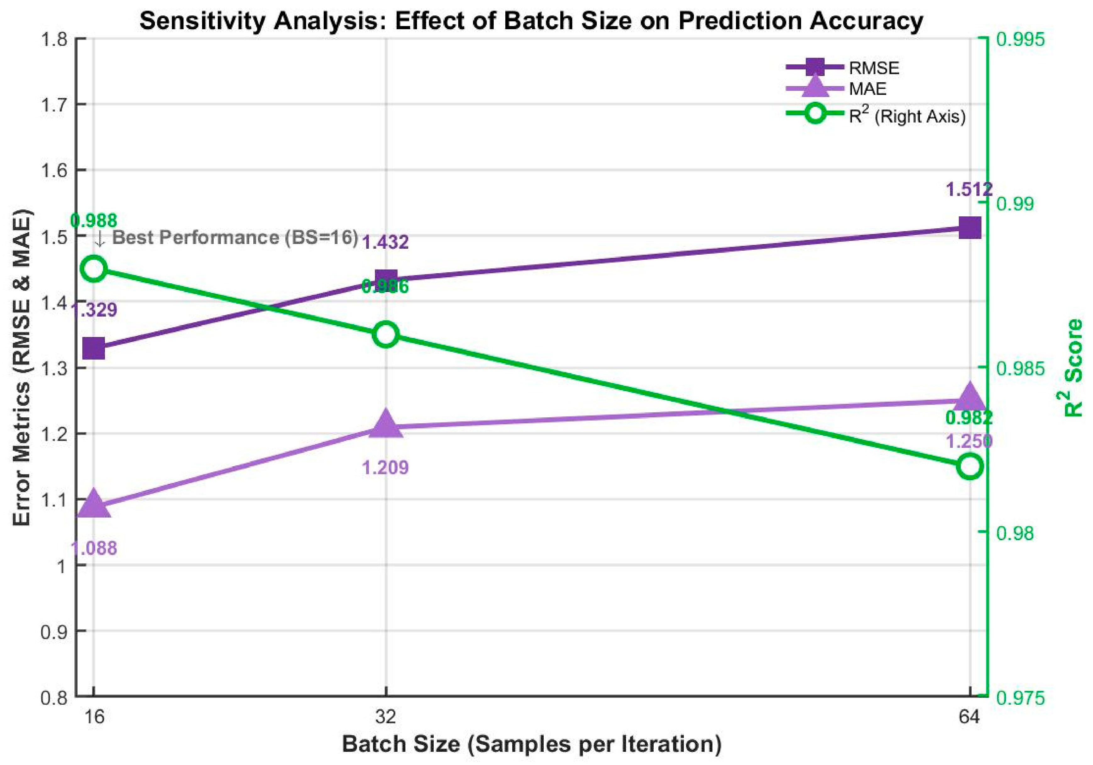
Table 7 lists the sensitivity analysis for the batch size configuration, with the evaluation results shown in Figure 16. The experimental findings indicate that a small batch size of 16 yields the highest predictive performance. This enhanced efficacy is primarily attributed to the increased frequency of parameter updates per epoch. This update rate introduces beneficial stochastic noise into the gradient descent pathway, thereby accelerating network convergence and facilitating escape from local minima. Conversely, increasing the batch size provides more consistent and deterministic gradient estimates; however, this expansion causes a slight deterioration in predictive accuracy. Optimization literature frequently attributes this behavior to the optimization trajectory settling into less adaptable regions of the solution space.
Table 8 presents the sensitivity analysis for the batch size configuration, with the evaluation findings depicted in Figure 17. Experimental findings show that a compact batch size of 16 delivers optimal predictive performance. This improved efficacy is mainly due to the accelerated rate of parameter updates per epoch. This operational rate introduces beneficial stochastic noise into the gradient descent trajectory. Subsequently, this noise accelerates network convergence and enables the model to escape local minima. Conversely, increasing the batch size offers more stable and deterministic gradient estimates. However, this expansion results in a negligible decrease in predictive accuracy, a behavior commonly attributed in optimization literature to the trajectory entering less adaptable regions of the solution space.
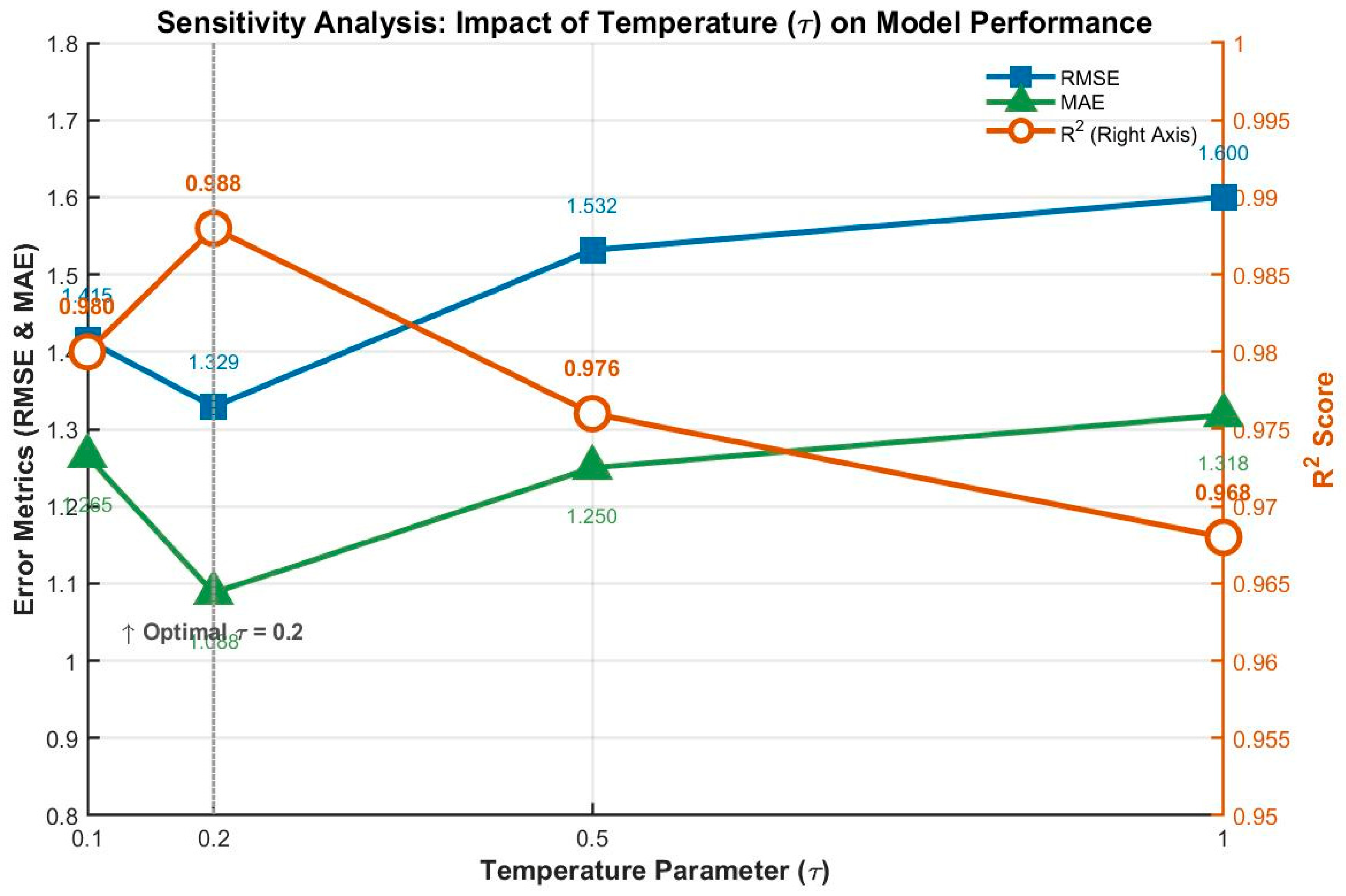
Table 9 summarizes the sensitivity analysis for the contrastive temperature parameter ( τ ), and the results of the evaluation are shown in Figure 18. The experiment shows that the best predictive performance is achieved at a temperature coefficient of 0.2. This means that the optimal parameter gives a moderate scaling of the sharpness of the distribution of similarity in the contrastive learning objective function. Such a modulation improves the generalization ability of the model. Also, this setting balances the penalty allocation of positive and negative example pairs in such a way as to prevent the contrastive loss from becoming too diffused which would hide important latent qualities but without putting too much emphasis on a small group of difficult negative pairs that would lead to optimization instability.


6. Discussion

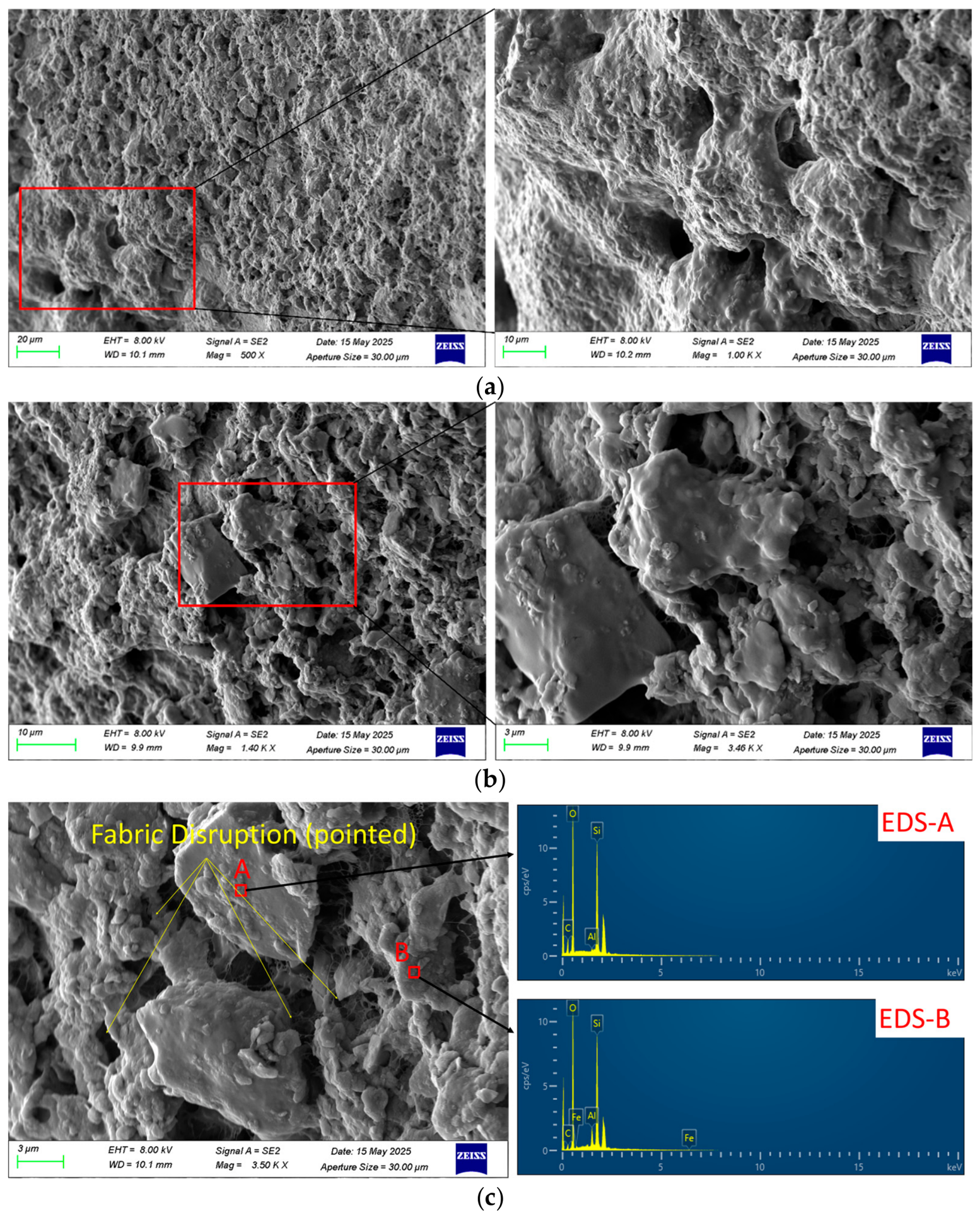
The mechanism underlying the shear strength evolution of seasonally frozen silty clay is elucidated via cryo-scanning electron microscopy (Cryo-SEM) and energy-dispersive spectroscopy (EDS). Direct evidence of fabric disruption and compositional heterogeneity induced by cyclic freeze thaw action is provided by the experimental results. Specifically, as explicitly indicated by the targeted annotations in Figure 19, the proliferation of micro fissures and the presence of detached particles are clearly revealed by the Cryo SEM micrographs. Concurrently, the redistribution of the pore network is fundamentally driven by ice segregation and cryo crystallization processes. Concurrently, EDS analysis delineates the precise spatial distribution of elements within the soil matrix.
These microscopic findings substantiate the macro-scale shear strength fluctuations predicted by the SSC-PINN model, thereby providing a rigorous micro-mechanical basis for the observed physical degradation of the soil fabric. To preserve the original soil structure and prevent shrinkage induced by moisture loss, a vacuum freeze drying technique was employed prior to the microscopic observation. The specimens were initially subjected to rapid freezing utilizing liquid nitrogen. The internal moisture was solidified instantly by this extreme cooling process, and structural damage caused by excessive ice crystal volume expansion was thereby minimized. Subsequently, the frozen samples were placed in a vacuum freeze dryer, where the solid ice was sublimated directly into water vapor under low temperature and high vacuum conditions. It is ensured by this desiccation procedure that the spatial arrangement of the soil particles, the natural inter fabric voids, and the micro fissure networks are completely maintained in their undisturbed state for the subsequent characterization. The Cryo-SEM micrographs display a highly heterogeneous and complex microstructure within the soil matrix.
At the initial stage of cyclic freeze–thaw exposure, the silty clay fabric exhibits a relatively high density characterized by well-bonded aggregate structures and minimal intergranular voids. However, repeated thermal cycling induces severe structural damage, manifesting as micro-fissures, the depletion of fine clay particles, and the formation of localized porous zones. These microstructural alterations indicate ice segregation, frost heaving, and mechanical fatigue, which drive the gradual deterioration of macro-scale shear strength. In particular, angular mineral grains observed within the fracture zones reflect physical abrasion and particle rearrangement driven by volumetric variations during the ice–water phase transition.
Complementary EDS analyses confirm the predominance of typical aluminosilicate mineral phases, with oxygen (O), silicon (Si), and aluminum (Al) serving as the primary constituent elements. Quantitative spectra indicate that the combined abundance of Si and O exceeds 70% in specific regions, a chemical signature indicative of mineral domains rich in quartz or illite. Trace elements, including iron (Fe), magnesium (Mg), potassium (K), and calcium (Ca), are periodically detected, signifying localized mineral weathering, secondary mineral precipitation, and solute migration during cyclic freezing and thawing. Notably, higher mass fractions of Fe and Ca are frequently exhibited by spectra extracted from fractured zones, as explicitly pointed out by the EDS B spectrum in Figure 18. These specific elemental signatures are strongly associated with clay mineral coatings or weakly cemented matrices. It is corroborated by existing microstructural investigations of frozen soils that such specific chemical compositions and weakly cemented structures are highly susceptible to crack propagation and mechanical deformation under thermal cycling [57].
These results highlight the inherent micro-scale variability of frozen soils, underscoring the necessity of employing physics-informed and representation-oriented deep learning approaches. In summary, a strong correlation exists between microstructural characteristics and the measured macroscopic degradation of shear strength. These characterizations justify the constitutive and architectural design choices of the proposed framework. The outcomes demonstrate that the macroscopic mechanical behavior of seasonally frozen soils is governed by micro-scale physical degradation mechanisms. Consequently, integrating these underlying mechanisms into the model architecture of the SSC-PINN framework significantly enhances both predictive accuracy and physical interpretability.
Furthermore, the outcomes derived from the proposed self-supervised contrastive physics-informed neural network are systematically compared with the existing literature to objectively validate the framework. It is explicitly demonstrated by recent studies on the mechanical degradation of seasonally frozen soils that conventional machine learning algorithms frequently fail to capture the complex non linear geomechanical behaviors induced by cyclic freezing and thawing [58,59]. Conversely, the superior predictive accuracy and robust physical interpretability of the proposed architecture are firmly corroborated by the comparative analysis presented in this study. Specifically, the accelerated shear strength deterioration observed during the initial freeze thaw cycles is perfectly aligned with the microstructural fatigue mechanisms documented in established geotechnical research [60]. Therefore, it is definitively validated by these objective comparisons that integrating physical constraints with representation learning provides significant advancements over traditional empirical and purely data-driven methodologies.
Finally, specific boundary conditions concerning the generalizability of the current findings must be explicitly acknowledged. The experimental evaluation and the subsequent model validation presented in this research are strictly confined to a single case study involving the seasonally frozen silty clay collected from the specified specific geographical region. Consequently, it is explicitly stated that broad generalizations are limited. The universal applicability of the proposed predictive framework to differing geological environments, alternative soil types, or distinct regional climatic conditions cannot be definitively guaranteed without further extensive validation. The necessity for future research incorporating diverse multisite datasets to systematically verify the generalized robustness of the algorithms is strongly highlighted by this limitation.

7. Conclusions

The innovative insights of this study are explicitly defined by the successful development of the self-supervised contrastive physics-informed neural network (SSC PINN) framework to systematically evaluate and predict the shear strength of seasonally frozen silty clay. By integrating self-supervised contrastive learning with physics-informed loss regularization, superior predictive accuracy is achieved by the proposed model. It is demonstrated by the experimental results that the extracted latent feature representations are effectively optimized by contrastive learning, while strict adherence to the governing constitutive laws of soil mechanics is ensured by the physics-informed objective function.
The critical contributions of both core components are firmly confirmed by the ablation studies. A significant performance degradation is observed when either the self-supervised contrastive module or the physics-based constraints are removed. Specifically, it is proven that the noise robustness of the extracted features is enhanced during the contrastive pretraining stage, whereas rigorous physical consistency is guaranteed by the physics-driven loss. Furthermore, the structural advantages of the proposed framework are highly emphasized by comparative evaluations against established baseline methods, including standard PINN, FSNN, RF, and SVR. It is quantitatively demonstrated by the obtained results that lower RMSE and MAE values, along with a superior coefficient of determination ( R 2 ), are consistently yielded by the SSC PINN architecture.
Finally, the generalizations of these conclusions must be appropriately moderated. It is explicitly restated that the specific geotechnical parameters and the associated degradation behaviors are strictly derived from the single case study involving the silty clay samples collected from Heilongjiang Province. Therefore, the direct extrapolation of these objective results to all silty clays in diverse seasonal frost regions is significantly limited. The efficacy of coupling data-driven representation learning with domain-specific physical principles is strongly underscored by this study. However, the universal applicability of the proposed methodology to varying geological materials must be rigorously validated by future multisite investigations and extended network optimization strategies.

Author Contributions

J.C.: Writing—original draft, Software, Methodology, Formal analysis, Validation. Z.W.: Writing—review & editing, Supervision, Conceptualization. S.C.: Writing—review & editing. G.X.: Writing—review & editing. H.W.: Funding acquisition. Y.M.: Project administration. X.T.: Project administration. All authors have read and agreed to the published version of the manuscript.

Funding

This research was funded by the China Geological Survey Applied Geological Survey Project, grant number DD20242171.

Institutional Review Board Statement

Not applicable.

Informed Consent Statement

Not applicable.

Data Availability Statement

Data will be made available on request.

Conflicts of Interest

The authors declare no conflict of interest.

References

  1. Lai, Y.; Xu, X.; Dong, Y.; Li, S. Present situation and prospect of mechanical research on frozen soils in China. Cold Reg. Sci. Technol. 2013, 87, 6–18. [Google Scholar] [CrossRef]
  2. Henry, H.A. Soil freeze–thaw cycle experiments: Trends, methodological weaknesses and suggested improvements. Soil Biol. Biochem. 2007, 39, 977–986. [Google Scholar] [CrossRef]
  3. Chen, H.; Du, H.; Guo, H.; Kong, F.; Zhang, Z. Freezing strain characteristics and mechanisms of unsaturated frozen soil: Analysis of matric suction and water–ice phase change. Acta Geotech. 2024, 19, 7243–7260. [Google Scholar] [CrossRef]
  4. Wang, B.; Xu, X.; Wang, X.; Gu, Q.; Chen, T. Mechanical behavior and strength criterion of frozen silty clay under complex stress paths. Geoderma 2023, 435, 116506. [Google Scholar] [CrossRef]
  5. Minasny, B.; Bandai, T.; Ghezzehei, T.A.; Huang, Y.C.; Ma, Y.; McBratney, A.B.; Widyastuti, M. Soil science-informed machine learning. Geoderma 2024, 452, 117094. [Google Scholar] [CrossRef]
  6. El Hariri, A.; Ahmed, A.E.E.; Kiss, P. Review on soil shear strength with loam sand soil results using direct shear test. J. Terramech. 2023, 107, 47–59. [Google Scholar] [CrossRef]
  7. Skempton, A.W.; Bishop, A.W. The measurement of the shear strength of soils. Geotechnique 1950, 2, 90–108. [Google Scholar] [CrossRef]
  8. Hongde, W.; Dongli, S.; Xiaoqin, S.; Shengqiang, T.; Yipeng, Z. Analysis of unsaturated shear strength and slope stability considering soil desalinization in a reclamation area in China. Catena 2021, 196, 104949. [Google Scholar] [CrossRef]
  9. Stefanow, D.; Dudziński, P.A. Soil shear strength determination methods–State of the art. Soil Tillage Res. 2021, 208, 104881. [Google Scholar] [CrossRef]
  10. Kim, B.S.; Shibuya, S.; Park, S.W.; Kato, S. Application of suction stress for estimating unsaturated shear strength of soils using direct shear testing under low confining pressure. Can. Geotech. J. 2010, 47, 955–970. [Google Scholar] [CrossRef]
  11. Brunori, F.; Penzo, M.C.; Torri, D. Soil shear strength: Its measurement and soil detachability. Catena 1989, 16, 59–71. [Google Scholar] [CrossRef]
  12. Nam, S.; Gutierrez, M.; Diplas, P.; Petrie, J. Determination of the shear strength of unsaturated soils using the multistage direct shear test. Eng. Geol. 2011, 122, 272–280. [Google Scholar] [CrossRef]
  13. Saliba, J.; Al-Shaar, W.; Delage, M. Comparison of field and laboratory tests for soil suitability assessment in raw earth construction. Appl. Sci. 2025, 15, 1932. [Google Scholar] [CrossRef]
  14. Li, T.; Tian, J.; Pei, X.; Guo, J.; Chen, M.; Xue, Y.; Meng, M. Shear strength indices predication model for coarse-grained soil based on particle gradation and moisture content information. Bull. Eng. Geol. Environ. 2025, 84, 344. [Google Scholar] [CrossRef]
  15. Hu, A.; Zhou, H.; Guo, F.; Wang, Q.; Zhang, J. Three-dimensional porous fibrous structural morphology changes of high-moisture extruded soy protein under the effect of moisture content. Food Hydrocoll. 2025, 159, 110600. [Google Scholar] [CrossRef]
  16. Liu, H.; Liu, H.; Xiao, Y.; McCartney, J.S. Effects of temperature on the shear strength of saturated sand. Soils Found. 2018, 58, 1326–1338. [Google Scholar] [CrossRef]
  17. Stark, T.D.; Hussain, M. Empirical correlations: Drained shear strength for slope stability analyses. J. Geotech. Geoenviron. Eng. 2013, 139, 853–862. [Google Scholar] [CrossRef]
  18. Guan, G.S.; Rahardjo, H.; Choon, L.E. Shear strength equations for unsaturated soil under drying and wetting. J. Geotech. Geoenviron. Eng. 2010, 136, 594–606. [Google Scholar] [CrossRef]
  19. Zhao, Y.; Li, X.; Liu, L. Measurement of unsaturated soil shear strength through drained-vented triaxial tests. J. Rock Mech. Geotech. Eng. 2025, 17, 5709–5727. [Google Scholar] [CrossRef]
  20. Karakul, H.; Ulusay, R. Empirical correlations for predicting strength properties of rocks from P-wave velocity under different degrees of saturation. Rock Mech. Rock Eng. 2013, 46, 981–999. [Google Scholar] [CrossRef]
  21. Rahman, T.; Sarkar, K. Lithological control on the estimation of uniaxial compressive strength by the P-wave velocity using supervised and unsupervised learning. Rock Mech. Rock Eng. 2021, 54, 3175–3191. [Google Scholar] [CrossRef] [PubMed]
  22. Fan, J.; Zhang, Y.; Zhou, W.; Yin, C. Landslide-tunnel interaction mechanism and numerical simulation during tunnel construction: A case from expressway in Northwest Yunnan Province, China. Arab. J. Geosci. 2022, 15, 1394. [Google Scholar] [CrossRef]
  23. Pan, R.; Yang, P.; Shi, X.; Zhang, T. Effects of freeze–thaw cycles on the shear stress induced on the cemented sand–structure interface. Constr. Build. Mater. 2023, 371, 130671. [Google Scholar] [CrossRef]
  24. Ping, S.; Wang, F.; Wang, D.; Li, S.; Yuan, Y.; Feng, G.; Shang, S. Multi-scale deterioration mechanism of shear strength of gypsum-bearing mudstone induced by water-rock reactions. Eng. Geol. 2023, 323, 107224. [Google Scholar] [CrossRef]
  25. Sheng, D.; Sloan, S.W.; Gens, A. A constitutive model for unsaturated soils: Thermomechanical and computational aspects. Comput. Mech. 2004, 33, 453–465. [Google Scholar] [CrossRef]
  26. Cavalcante, A.L.B.; Mascarenhas, P.V.S. Efficient approach in modeling the shear strength of unsaturated soil using soil water retention curve. Acta Geotech. 2021, 16, 3177–3186. [Google Scholar] [CrossRef]
  27. Cai, W.; Zhu, C. Constitutive model for thermo–hydro–mechanical behaviors of saturated partially frozen cohesionless soils: A theoretical pore-scale study. J. Geotech. Geoenviron. Eng. 2024, 150, 04024007. [Google Scholar] [CrossRef]
  28. Pham, T.A.; Sutman, M. Modeling the combined effect of initial density and temperature on the soil–water characteristic curve of unsaturated soils. Acta Geotech. 2023, 18, 6427–6455. [Google Scholar] [CrossRef]
  29. Chen, L.; Ming, F.; Zhang, X.; Wei, X.; Liu, Y. Comparison of the hydraulic conductivity between saturated frozen and unsaturated unfrozen soils. Int. J. Heat Mass Transf. 2021, 165, 120718. [Google Scholar] [CrossRef]
  30. Bai, R.; Lai, Y.; Zhang, M.; Yu, F. Theory and application of a novel soil freezing characteristic curve. Appl. Therm. Eng. 2018, 129, 1106–1114. [Google Scholar] [CrossRef]
  31. Zhang, Y.; Zhang, P. Physics-informed data-driven modelling and computation in geotechnics. Georisk 2026, 1–16. [Google Scholar] [CrossRef]
  32. Wang, W.; Kosakowski, G.; Kolditz, O. A parallel finite element scheme for thermo-hydro-mechanical (THM) coupled problems in porous media. Comput. Geosci. 2009, 35, 1631–1641. [Google Scholar] [CrossRef]
  33. Zhang, T.; Wang, D.; Lu, Y. RheologyNet: A physics-informed neural network solution to evaluate the thixotropic properties of cementitious materials. Cem. Concr. Res. 2023, 168, 107157. [Google Scholar] [CrossRef]
  34. Amini, D.; Haghighat, E.; Juanes, R. Physics-informed neural network solution of thermo–hydro–mechanical processes in porous media. J. Eng. Mech. 2022, 148, 04022070. [Google Scholar] [CrossRef]
  35. Rezaei, S.; Moeineddin, A.; Kaliske, M.; Apel, M. Integration of physics-informed operator learning and finite element method for parametric learning of partial differential equations. arXiv 2024, arXiv:2401.02363. [Google Scholar]
  36. Chen, H.; Ding, Q.; Guo, H.; Li, J.; Gao, X.; Li, S. Shear strength model of unsaturated frozen soil based on soil freezing characteristic and soil water characteristic. Cold Reg. Sci. Technol. 2024, 219, 104132. [Google Scholar] [CrossRef]
  37. Wang, Z.; Zhang, Y.; Zhang, C.; Li, B. Revealing the melting mechanism of segregated ice in frozen soil based on visualizing mass transfer dynamics. Cold Reg. Sci. Technol. 2025, 239, 104558. [Google Scholar] [CrossRef]
  38. Gao, Q.; Wen, Z.; Zhou, Z.; Brouchkov, A.; Wang, D.; Shi, R. A creep model of pile-frozen soil interface considering damage effect and ice effect. Int. J. Damage Mech. 2022, 31, 3–21. [Google Scholar] [CrossRef]
  39. Arenson, L.U.; Springman, S.M.; Sego, D.C. The rheology of frozen soils. Appl. Rheol. 2007, 17, 12147. [Google Scholar] [CrossRef]
  40. Raissi, M.; Perdikaris, P.; Karniadakis, G.E. Physics-informed neural networks: A deep learning framework for solving forward and inverse problems involving nonlinear partial differential equations. J. Comput. Phys. 2019, 378, 686–707. [Google Scholar] [CrossRef]
  41. Chen, Z.; Liu, Y.; Sun, H. Physics-informed learning of governing equations from scarce data. Nat. Commun. 2021, 12, 6136. [Google Scholar] [CrossRef] [PubMed]
  42. Karniadakis, G.E.; Kevrekidis, I.G.; Lu, L.; Perdikaris, P.; Wang, S.; Yang, L. Physics-informed machine learning. Nat. Rev. Phys. 2021, 3, 422–440. [Google Scholar] [CrossRef]
  43. Sun, Y.; Pang, S.; Li, H.; Qiao, S.; Zhang, Y. Enhanced lithology classification using an interpretable SHAP model integrating semi-supervised contrastive learning and transformer with well logging data. Nat. Resour. Res. 2025, 34, 785–813. [Google Scholar] [CrossRef]
  44. Jeremiah, J.J.; Abbey, S.J.; Booth, C.A.; Kashyap, A. Results of application of artificial neural networks in predicting geo-mechanical properties of stabilised clays—A review. Geotechnics 2021, 1, 147–171. [Google Scholar] [CrossRef]
  45. Wang, S.; Teng, Y.; Perdikaris, P. Understanding and mitigating gradient flow pathologies in physics-informed neural networks. SIAM J. Sci. Comput. 2021, 43, A3055–A3081. [Google Scholar] [CrossRef]
  46. Bouclier, R.; Bonnet–Eymard, R.; Rabineau, E.; Réthoré, J. PINN-based identification of spatially varying elastic moduli from experimental full-field displacement data. Comput. Methods Appl. Mech. Eng. 2026, 455, 118874. [Google Scholar] [CrossRef]
  47. Lee, M. GELU activation function in deep learning: A comprehensive mathematical analysis and performance. arXiv 2023, arXiv:2305.12073. [Google Scholar]
  48. Al-Atroush, M.E. A deep learning physics-informed neural network (PINN) for predicting drilled shaft axial capacity. Appl. Comput. Geosci. 2025, 26, 100246. [Google Scholar] [CrossRef]
  49. Guo, H.; Sun, Y.; Sun, C.; Gu, H. Experimental study on shear strength and deterioration behavior of silty clay under dry-wet-freeze-thaw cycles. Sci. Rep. 2025, 15, 17907. [Google Scholar] [CrossRef] [PubMed]
  50. Rasti, A.; Pineda, M.; Razavi, M. Assessment of soil moisture content measurement methods: Conventional laboratory oven versus halogen moisture analyzer. J. Soil Water Sci. 2020, 4, 151–160. [Google Scholar] [CrossRef]
  51. Elsawy, M.B.; Alsharekh, M.F.; Shaban, M. Modeling undrained shear strength of sensitive alluvial soft clay using machine learning approach. Appl. Sci. 2022, 12, 10177. [Google Scholar] [CrossRef]
  52. Wang, X.; Yi, S.; Gu, H.; Xu, J.; Xu, W. WF-PINNs: Solving forward and inverse problems of burgers equation with steep gradients using weak-form physics-informed neural networks. Sci. Rep. 2025, 15, 40555. [Google Scholar] [CrossRef] [PubMed]
  53. Seidi, E.; Kaviari, F.; Miller, S.F. Hyperparameter tuning of artificial neural network-based machine learning to optimize number of hidden layers and neurons in metal forming. J. Manuf. Mater. Process. 2025, 9, 260. [Google Scholar] [CrossRef]
  54. Abdulameer, A.; Hassan, R.F.; Humadi, A.F. The impact of batch size on skin cancer classification using ResNet18. Dijlah J. Eng. Sci. 2025, 2. [Google Scholar] [CrossRef]
  55. Keller, A.; Kuo, F.Y.; Nuyens, D.; Sloan, I.H. Regularity and tailored regularization of deep neural networks, with application to parametric PDEs in uncertainty quantification. arXiv 2025, arXiv:2502.12496. [Google Scholar]
  56. Li, J.; Wang, Y.; Zhang, X.; Jiang, D.; Dai, W.; Li, C.; Tian, Q. Contrastive learning via variational information bottleneck. IEEE Trans. Pattern Anal. Mach. Intell. 2025, 47, 7410–7427. [Google Scholar] [CrossRef] [PubMed]
  57. Xu, W.; Wang, X. Effect of freeze–thaw cycles on mechanical strength and microstructure of silty clay in the Qinghai–Tibet Plateau. J. Cold Reg. Eng. 2022, 36, 04021018. [Google Scholar] [CrossRef]
  58. Memiş, M.A.; Keskin, I.; Demir, S.; Memiş, Ş.U. Machine learning-based prediction of permafrost degradation and its implications on geotechnical infrastructure: A comprehensive review. AI Civ. Eng. 2025, 4, 28. [Google Scholar] [CrossRef]
  59. Luo, H.; Han, F.; Liu, F.; Yu, W.; Liang, T.; Wang, S. Interpretable machine learning for thermomechanical property prediction of geopolymer-solidified soils under subzero curing conditions. J. Cold Reg. Eng. 2026, 40, 04025048. [Google Scholar] [CrossRef]
  60. Chen, K.; Huang, S.; Li, X.; Liu, H.; Yang, Y.; Liu, Y.; Ding, L. Compression strength and damage model of frozen silty clay in Xing’an Baikal permafrost under temperature effects. Sci. Rep. 2025, 15, 22091. [Google Scholar] [CrossRef] [PubMed]
Figure 1. Multiscale geographical localization of the study area illustrating the position of Heilongjiang Province within the national territory of China (a), and the specific sampling location within the provincial administrative boundaries (b), alongside macroscopic representations of the undisturbed silty clay samples (c).
Applsci 16 07746 g001
Figure 2. Granulometric curve of the tested seasonally frozen silty clay. The blue dashed lines indicate the boundaries between the different soil particle size classifications.
Applsci 16 07746 g002
Figure 3. The appearance of the frozen soil specimens. (a) Compactor and compacted soil sample; (b) Soil samples after freezing.
Applsci 16 07746 g003
Figure 4. Overall methodological framework.
Applsci 16 07746 g004
Figure 5. The neural network design of SSC-PINN.
Applsci 16 07746 g005
Figure 6. Flowchart of physical constraint evaluation.
Applsci 16 07746 g006
Figure 7. Flowchart of Data Augmentation and Generation of Contrastive Sample.
Applsci 16 07746 g007
Figure 8. Test results of 100 samples (a) 25 samples with a water content of 18%; (b) 25 samples with a moisture content of 20%; (c) 25 samples with a moisture content of 22%; (d) 25 samples with a water content of 24%.
Applsci 16 07746 g008aApplsci 16 07746 g008b
Figure 9. The R 2 , RMSE, and MAEvalues of the six models. (a) R 2 , (b) RMSE, and (c) MAE.
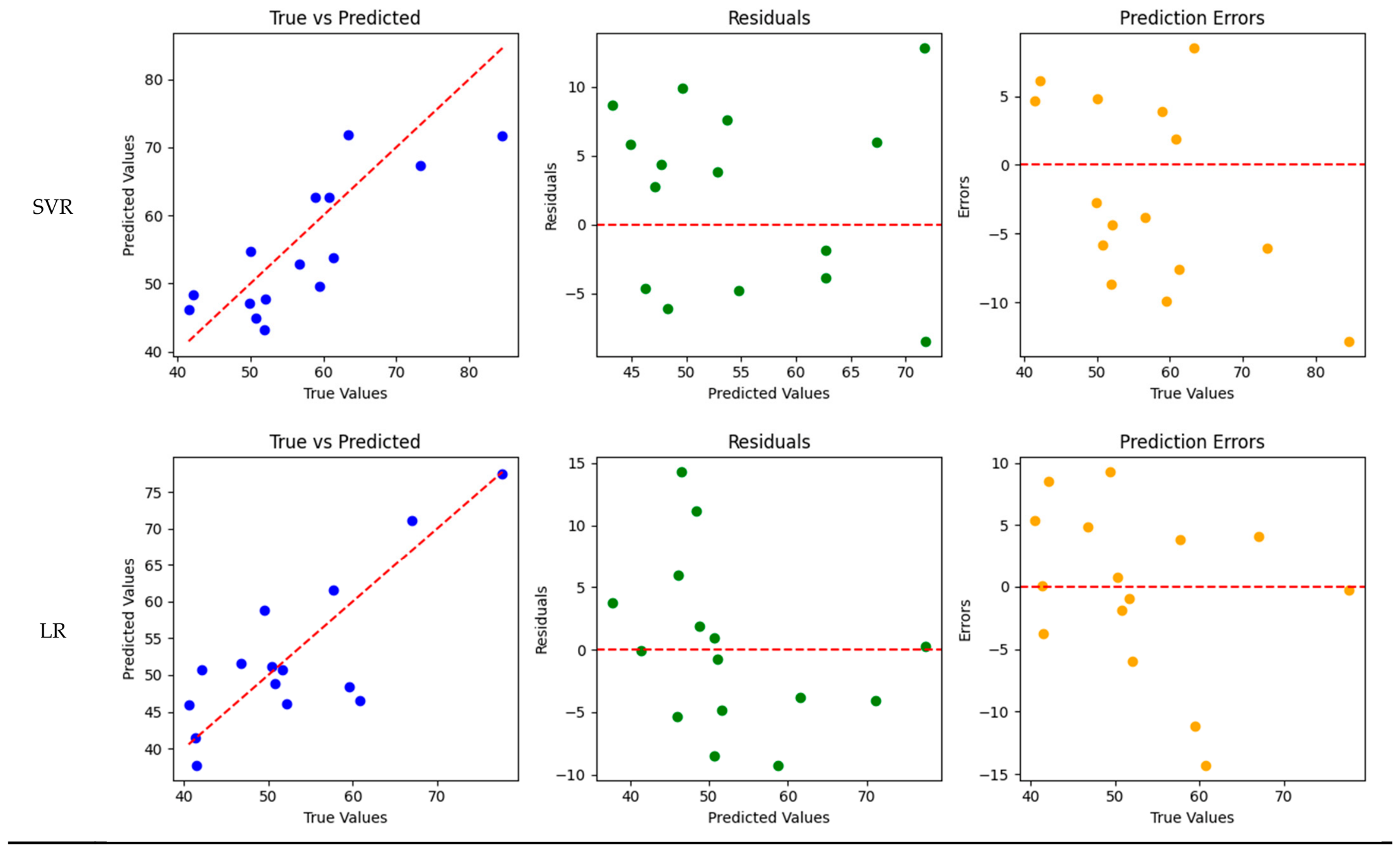
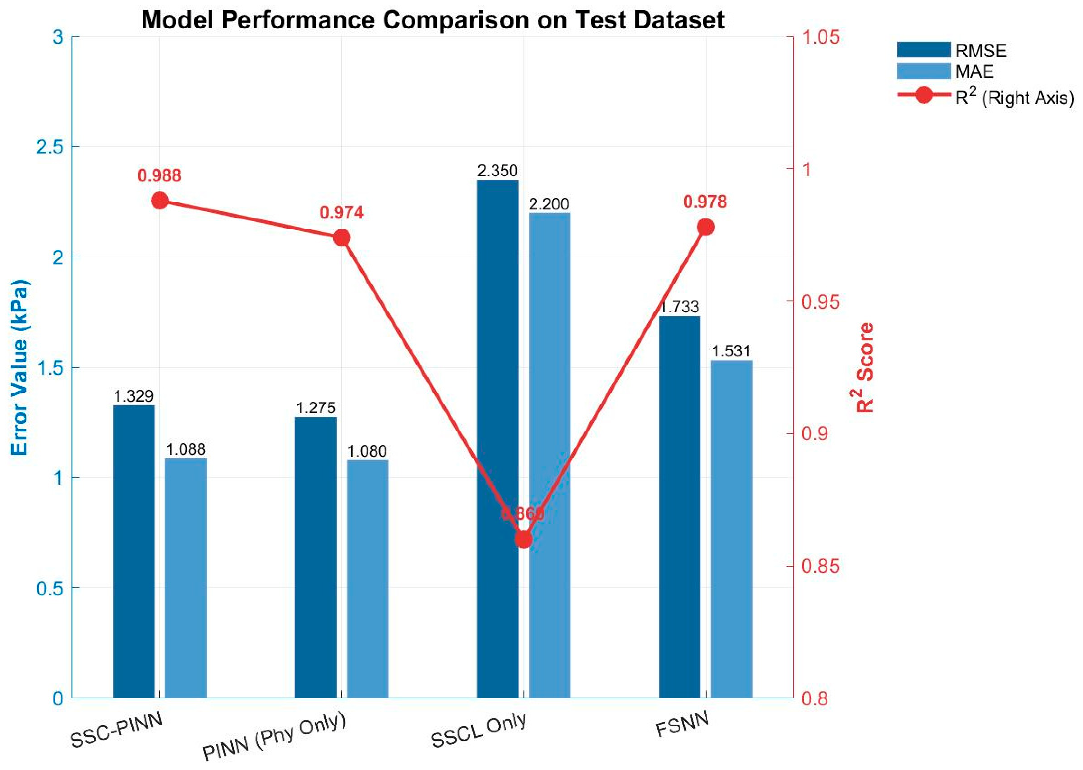
Applsci 16 07746 g009aApplsci 16 07746 g009b
Figure 10. The loss curve for the SSC-PINN model.
Applsci 16 07746 g010
Figure 11. Scatter plots, residual plots and error plots of the six models.
Applsci 16 07746 g011aApplsci 16 07746 g011b
Figure 12. The R 2 , RMSE, and MAE values of the ablation models.
Applsci 16 07746 g012
Figure 13. Sensitivity analysis of the learning rate parameter.
Applsci 16 07746 g013
Figure 14. Sensitivity analysis of the Number of Hidden Layers parameter.
Applsci 16 07746 g014
Figure 15. Sensitivity analysis of neurons per layer parameters.
Applsci 16 07746 g015
Figure 16. The sensitivity analysis of the batch size parameter.
Applsci 16 07746 g016
Figure 17. The sensitivity analysis of the weight decay parameter.
Applsci 16 07746 g017
Figure 18. The sensitivity analysis of the temperature parameter.
Applsci 16 07746 g018
Figure 19. Microstructural and compositional characterization of the tested silty clay sample. (a) A low magnification Cryo SEM micrograph illustrating the general pore network and macroscale surface morphology. (b) A high magnification Cryo SEM micrograph detailing localized fabric disruption, micro fissures, and detached particles. (c) Energy dispersive spectroscopy spectra extracted from specific regions marked in the matrix, verifying the compositional heterogeneity induced by cyclic freezing and thawing.
Applsci 16 07746 g019
Table 1. Physical properties table of soil in the seasonal frozen area.
Natural density/(g·cm−3)1.53
Dry density/(g·cm−3)1.21
Natural moisture content/%21.3~37.1
Liquid limit/%40.76
Plastic limit/%28.14
Plasticity index12.62
Optimum moisture content/%19.61
Maximum dry density/(g·cm−3)1.61
Average permeability coefficient/(cm·s−1)1.01 × 10−4
Table 2. The R 2 , RMSE, and MAE values of the six models.
ModelsTrain R 2 Val R 2 Test R 2 Train RMSEVal RMSETest RMSETrain MAEVal MAETest MAE
SSC-PINN0.9990.9870.9880.2121.2631.3290.1680.9981.088
PINN0.9990.9860.9740.1581.3631.2750.1111.1181.080
FSNN0.9990.9660.9780.1311.6491.7330.1001.5021.531
RF0.9980.9840.9750.4291.2321.7010.2990.9761.147
SVR0.6970.6930.6016.5616.2736.6335.4264.9685.693
LR0.6550.6060.7786.8505.6145.5045.6394.6324.566
Table 3. The R 2 , RMSE, and MAE values of the ablation models.
ModelsTest R 2 Test RMSETest MAE
SSC-PINN0.9881.3291.088
PINN (Physics-Informed Loss Only)0.9741.2751.080
Self-Supervised Contrastive Learning Only (No Physics Loss)0.8602.3502.200
Fully Supervised Neural Network (FSNN)0.9781.7331.531
Table 4. Sensitivity analysis of the learning rate parameter.
Learning Rate Test R2 Test RMSE Test MAE
0.00010.9821.3421.239
0.0010.9881.3291.088
0.010.9751.6651.431
0.10.9602.1201.742
Table 5. Sensitivity analysis of the Number of Hidden Layers parameter.
Number of Hidden LayersTest R 2 Test RMSETest MAE
20.9701.5121.319
30.9881.3291.088
40.9821.4121.250
50.9761.5321.362
Table 6. Sensitivity analysis of neurons per layer parameters.
Neurons per LayerTest R 2 Test RMSETest MAE
320.9651.5801.400
640.9881.3291.088
1280.9811.3751.202
2560.9741.5121.250
Table 7. The sensitivity analysis of the batch size parameter.
Batch SizeTest R 2 Test RMSETest MAE
160.9881.3291.088
320.9861.4321.209
640.9821.5121.250
Table 8. The sensitivity analysis of the weight decay parameter.
Weight DecayTest R 2 Test RMSETest MAE
0.010.9751.4501.317
0.0010.9881.3291.088
0.00010.9861.4551.220
Table 9. The sensitivity analysis of the temperature parameter.
TemperatureTest R 2 Test RMSETest MAE
0.10.9801.4151.265
0.20.9881.3291.088
0.50.9761.5321.250
1.00.9681.6001.318
Disclaimer/Publisher’s Note: The statements, opinions and data contained in all publications are solely those of the individual author(s) and contributor(s) and not of MDPI and/or the editor(s). MDPI and/or the editor(s) disclaim responsibility for any injury to people or property resulting from any ideas, methods, instructions or products referred to in the content.