A Multi-Feature Early Fusion Network with Domain-Specific Contrastive Representation and Attention Mechanism for Side-Scan Sonar Target Detection

Abstract

Accurate target detection in side-scan sonar imagery is important for marine resource investigation, underwater infrastructure inspection, and maritime security. However, Side-scan sonar images are often affected by low contrast, acoustic speckle, weak target boundaries, and cluttered seabed backgrounds, which make target detection particularly challenging, especially under limited training data conditions. To improve the representation of sonar-specific structures, this study proposes a multi-feature early fusion detection network, referred to as MFEF-Det, for side-scan sonar target detection. The method combines multiple handcrafted features with data-driven representations to provide complementary information. In particular, a directional contrast core response feature (DCCR) is introduced to better emphasize the echo–shadow structure commonly observed in side-scan sonar imagery. An adaptive fusion strategy is then adopted to combine multiple feature maps before feeding them into a detection network, and an attention refinement module is further employed for complex scenes to improve the discrimination between target-related regions and cluttered backgrounds. Experiments were conducted on two publicly available sonar datasets. Experiments on the KLSG and SSS-Bottom datasets demonstrate that MFEF-Det achieves 0.933 ± 0.016 mAP@0.5 and 0.866 ± 0.052 mAP@0.5, respectively. The results indicate that the proposed feature representation can improve detection performance in both relatively clean and more challenging noisy scenes. These findings suggest that incorporating sonar-specific priors can be beneficial for side-scan sonar detection in marine survey and maritime-security applications.

1. Introduction

With the growing demands of marine resource development and maritime security, efficient and accurate underwater target detection technologies have become increasingly important. Compared to other acoustic devices, side-scan sonar (SSS) offers wider swath coverage, higher imaging resolution, compact size, and lower cost, enabling effective acquisition of seabed information. It plays a vital role in marine geological surveys, seabed geomorphology classification, sediment detection, underwater archaeology, and national defense security [1,2]. However, due to the complex underwater environment and the unique characteristics of acoustic wave propagation, sonar images often exhibit low contrast, unclear target contours, and severe noise interference. These factors pose significant challenges to the efficiency and accuracy of target extraction from side-scan sonar images.

Compared to common optical images, side-scan sonar target detection faces three main challenges:

(1)

Differences in imaging mechanisms. Side-scan imaging relies on seabed backscattering and employs a push-broom slant-range imaging model, which differs significantly from optical imaging based on visible light, increasing the difficulty of side-scan target detection.

(2)

Small sample size. Although seabed targets are diverse, the vastness of the seafloor limits the number of detectable targets obtained from multiple surveys, making target detection under small-sample conditions considerably more challenging.

(3)

Inconspicuous features and scattered distribution. Compared to the background, side-scan target pixels are less prominent, and the texture information on target surfaces is difficult to fully capture under acoustic imaging. Moreover, the scattered distribution of seabed targets further exacerbates detection difficulties.

Early sonar target detection methods relied mainly on handcrafted features and classical classifiers [3,4,5]. Various feature descriptors have been explored, including statistical features [6,7], morphological features, and pixel-based features [8]. For instance, some studies utilized gray-level co-occurrence matrices to extract texture features from side-scan sonar images and combined them with Support Vector Machine (SVM) algorithms for image classification [7]. Another study proposed an Adaboost classifier based on fractal texture features for shipwreck detection [9]. While these methods achieve certain effectiveness in specific scenarios, they primarily rely on manually designed feature extractors, which exhibit notable limitations when handling complex and variable marine environments. Traditional single-feature detection methods struggle to balance detection accuracy and robustness when confronted with complex seabed scenes.

The introduction of deep learning has brought revolutionary changes to this field. In the current research landscape of target detection based on side-scan sonar images, mainstream research directions primarily focus on the improvement and optimization of pure deep learning models [10,11], especially single-stage detectors represented by the YOLO series. Researchers customize and refine the backbone network, feature fusion network, and detection head of these models by introducing various advanced computer vision techniques, aiming to better adapt to the characteristics of sonar images [12,13,14,15,16]. Numerous improvements have been made to different versions of YOLO [17,18] to address the specificities of sonar imagery. Side-scan sonar images contain not only visual information but also physical acoustic properties. Existing CNNs that directly process raw grayscale images often lose high-frequency texture details and weak edge information during down-sampling, particularly when the seabed background is complex.

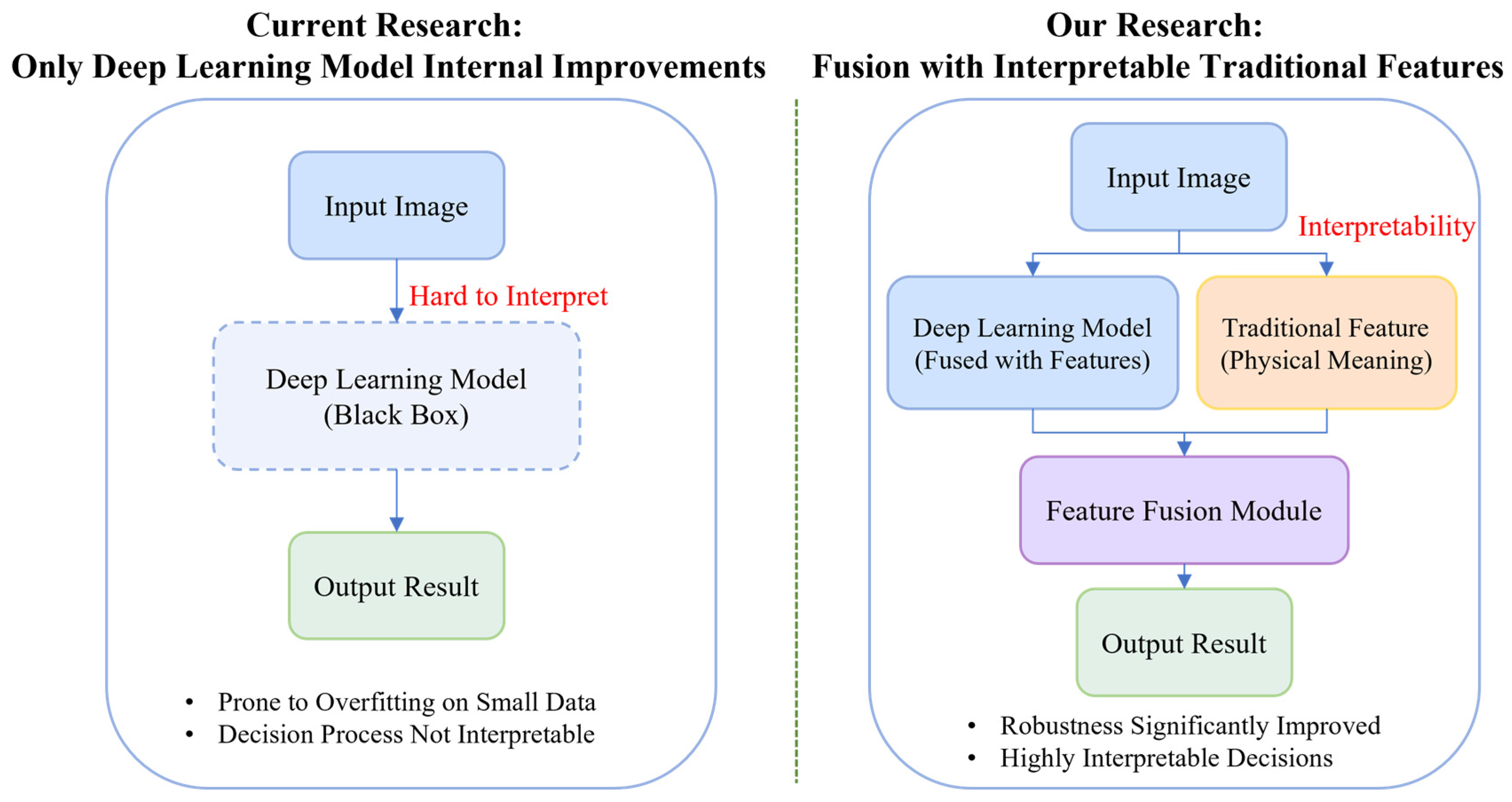
In the field of side-scan sonar, the potential research value and future directions of directly fusing traditional features with deep learning features are clear. As shown in Figure 1, traditional handcrafted features, such as HOG and LBP, while having limited expressive power in complex scenes, are designed based on human understanding of low-level image structures. They possess clear physical meaning and good interpretability. In certain specific situations, such as when the contrast between target and background is low, or when the target is partially occluded, these low-level features may provide critical information that deep learning models struggle to learn automatically. Although deep learning models are powerful, their “black box” nature makes their decision-making process difficult to fully comprehend, and they may sometimes learn spurious correlations unrelated to the task. Therefore, integrating highly interpretable traditional features into deep learning models holds promise for improving model robustness and generalization capability, especially in scenarios with small samples or imbalanced data distributions.

To the best of our knowledge, fusing traditional features with deep learning features for side-scan sonar target detection remains a relatively under-explored area [19,20,21,22,23,24,25]. Instead of employing generic object detection methods for side-scan sonar images, this work investigates an early fusion network for side-scan sonar target detection that integrates sonar-oriented handcrafted features with a deep detector. A directional contrast core response feature is introduced to emphasize the echo–shadow relationship that is characteristic of many sonar targets. Multiple standard handcrafted features are also evaluated, and their combinations are systematically studied. In addition, an attention module is used to adaptively suppress irrelevant responses when the fused features become redundant or noisy. The main contributions of this study are as follows:

(1)

We propose MFEF-Det, a multi-feature early fusion detector designed for side-scan sonar imagery. Rather than relying only on raw intensity images, the network integrates raw sonar intensity with domain-informed structural representations at the input stage, enabling the detector to preserve complementary intensity, boundary, and local contrast information before deep feature extraction.

(2)

To explicitly capture the characteristic highlight–shadow transitions –produced by sonar targets, a directional contrast core response feature is introduced. DCCR suppresses slowly varying seabed background responses while enhancing directional local contrast around target-related highlight-shadow structures. This representation provides complementary information to conventional gradient and edge descriptors.

(3)

An early channel-wise fusion mechanism is employed to allow the backbone to jointly learn from raw and handcrafted feature representations from the first convolutional layers. The proposed design achieves an mAP@0.5 of 0.866, substantially outperforming the sum fusion strategy.

(4)

Extensive experiments under a unified training protocol, repeated across three random seeds, demonstrate that MFEF-Det achieves 0.933 ± 0.016 mAP@0.5 on KLSG and 0.866 ± 0.052 on SSS-Bottom.

2. Materials and Methods

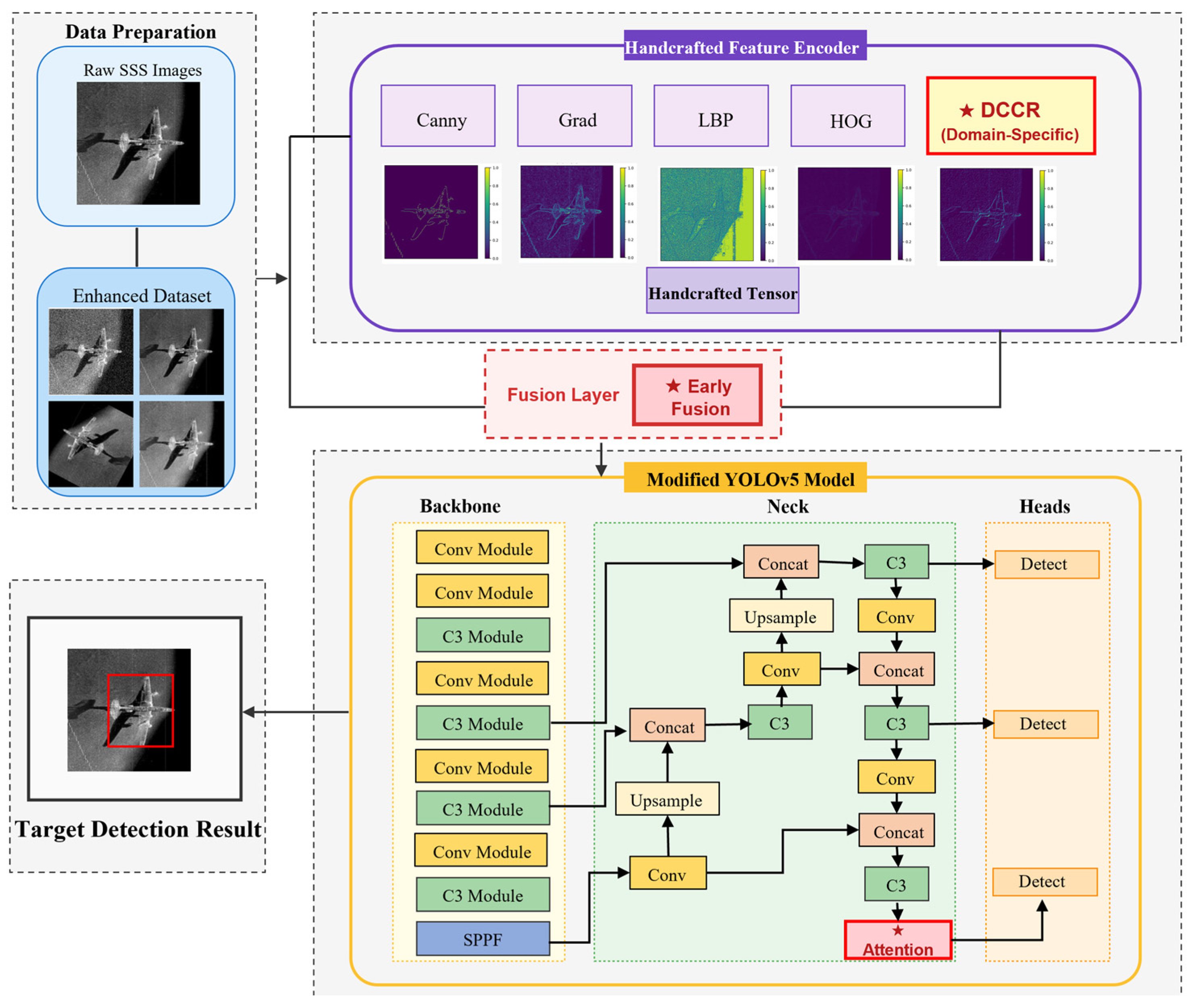
To overcome the limitations of existing sonar image detection methods, we propose a novel sonar image detection network named MFEF-Det. MFEF-Det employs a small target detection network for side-scan sonar images based on adaptive multi-stream feature fusion and attention enhancement. First, a domain-customised feature representation is defined, which together with four traditional features constitutes a handcrafted feature set. Second, a two-level adaptive fusion mechanism is designed. It first performs optimized fusion within the handcrafted feature set and then conducts fusion between these features and data-driven deep semantic features. Finally, accurate recognition is achieved through an attention-guided detection network. In this section, we primarily present the details of proposed method. Initially, we outline the overall structure of the network. Subsequently, Section 2.1, Section 2.2, Section 2.3, Section 2.4, Section 2.5 and Section 2.6 elaborates on the architecture used in the network, including the data preprocessing module, the DCCR feature extractor, the multi-stream feature extraction module, and the attention-enhanced detection module.

2.1. The Overall Architecture of MFEF-Det

The overall architecture of the proposed MFEF-Det is shown in Figure 2. MFEF-Det consists of a data preprocessing module, a DCCR feature extractor, a multi-stream feature extraction module, and an attention-enhanced detection module. Specifically, in the data preprocessing module, operations such as geometric transformation, noise injection, and contrast enhancement are applied to the original side-scan sonar images to construct an enhanced dataset that simulates complex underwater imaging conditions, providing a robust foundation for subsequent feature learning. The multi-stream feature extraction module performs feature encoding in parallel. In the handcrafted feature stream, the innovatively designed DCCR feature extractor in this work is specifically used to capture the unique scattering and structural patterns of sonar images. Together with four classic visual features, it forms a highly complementary composite feature vector embedded with domain knowledge. In the deep learning feature stream, a convolutional neural network automatically learns high-level semantics and global contextual information from the raw images. The features from the two streams are spatially aligned, laying the groundwork for subsequent fusion. Specifically, the fused input has a dimension of (H, W, 3 + N). The first convolution layer of the YOLOv5 backbone was modified to accept 3 + N channels. In order to bolster the model’s capability in capturing critical features while mitigating background interference, The Convolutional Block Attention Module was incorporated into the terminal stage of the P5 branch in the YOLOv5 head. The CBAM is sequentially integrated after the last C3 module and prior to the Detect layer. This architecture facilitates the refinement of high-level semantic features through joint channel and spatial attention mechanisms. The multi-scale detection head further ensures sensitivity to small targets of varying sizes.

2.2. Data Processing Module

To improve robustness, data augmentation methods are applied to the training images, including random scaling, translation, cropping, flipping, and geometric distortion. In addition, in order to deal with the class imbalance problem, CC-WGAN-generated [26] samples were used only in the training partition, with emphasis on minority classes. No synthetic data were included in validation or test sets, preventing leakage. Image preprocessing enriches the diversity of the data and improves the generalization performance of the network.

2.3. DCCR Feature Extractor

The directional contrast core response is designed to model local directional contrast in sonar images. Its purpose is to emphasize the structural relationship between target echoes and surrounding acoustic shadows, which is often informative in side-scan sonar imagery. The design of DCCR is motivated by the local acoustic structure of side-scan sonar targets. A target commonly produces a high-intensity highlight adjacent to a low-intensity acoustic shadow, which forms a directional local contrast pattern. In locally smooth background regions, directional difference responses are close to zero. In contrast, at highlight–shadow boundaries, the directional contrast response becomes large. Therefore, directional contrast kernels suppress slowly varying seabed background while emphasizing target-related structural transitions. Combining horizontal and vertical responses reduces sensitivity to target orientation and provides a compact, domain-informed representation complementary to the raw sonar intensity image. Unlike Canny and conventional gradient features, DCCR is designed to retain the contrast relationship between the highlight and its surrounding shadow rather than only isolated edge magnitude.

Given an input image I(x, y), contrast kernels in the horizontal and vertical directions are defined, and the corresponding responses are computed by two-dimensional convolution.

$$K_h=\left[\begin{array}{cc}1& 1\\ -1& -1\end{array}\right], K_v=\left[\begin{array}{cc}1& -1\\ 1& -1\end{array}\right]$$

(1)

where $K_h$ and $K_v$ are the horizontal and vertical convolution kernels, respectively.

The corresponding directional contrast responses are obtained by convolving the input image I(x, y) with these kernels:

$$R_h(x,y)=I(x,y)\ast K_h, R_v(x,y)=I(x,y)\ast K_v$$

(2)

where ∗ denotes the 2D convolution operation; and R_h(x, y) and R_v(x, y) are the horizontal and vertical contrast response maps, respectively.

The final DCCR response is obtained by combining the absolute values of the two directional responses:

$${\mathrm{R}}_{\mathrm{DCCR}}{(\mathrm{x},\mathrm{y}) = |\mathrm{R}}_{\mathrm{h}}{(\mathrm{x},\mathrm{y})| + |\mathrm{R}}_{\mathrm{v}}(\mathrm{x},\mathrm{y})|$$

(3)

where ∣·∣ denotes the absolute value operator, and ${\mathrm{R}}_{\mathrm{DCCR}}(\mathrm{x},\mathrm{y})$ is the raw directional contrast response map before normalization.

To facilitate comparability across different image regions and enable consistent fusion with other features, the response map is normalized to the range [0, 1]:

$${\widehat{R}}_{DCCR}(x,y)={\displaystyle \frac{R_{DCCR}(x,y)}{\max (R_{DCCR})}}$$

(4)

where $\max (R_{DCCR})$ denotes the maximum value of $R_{DCCR}$ over the entire spatial domain, and ${\widehat{R}}_{DCCR}(x,y)$ is the normalized DCCR feature map, which serves as one of the five input channels in the subsequent early fusion stage.

Compared with generic edge operators, this feature is intended to retain directional contrast information related to sonar imaging structure rather than merely emphasizing local intensity changes.

2.4. Multi-Stream Feature Extraction Module

In addition to DCCR, four commonly used handcrafted features are considered: gradient magnitude, Canny edges, local binary pattern (LBP), and histogram of oriented gradients (HOG). These features capture different aspects of image structure and are used to study whether complementary low-level information can improve target detection.

(1)

Gradient Magnitude Calculation

Gradient magnitude reflects local intensity variation and is commonly used to describe edge strength. For the input acoustic intensity image I(x, y), Sobel operators are used to compute the horizontal and vertical gradients:

$$G_x(x,y)=I(x,y)\ast S_x,G_y(x,y)=I(x,y)\ast S_y$$

(5)

where ∗ denotes the 2D convolution operation; (x, y) is the pixel spatial coordinate; $S_x$ and $S_y$ are the horizontal and vertical Sobel kernel matrices, respectively; $G_x(x,y)$ and $G_y(x,y)$ are the corresponding horizontal and vertical gradient maps.

The gradient magnitude M(x, y) is obtained by computing the Euclidean norm:

$$M(x,y)=\sqrt{G_x^2(x,y)+G_y^2(x,y)}$$

(6)

The result is normalized to the range [0, 1].

(2)

Canny Edge Feature Extraction

The Canny detector is used to generate a thin binary edge map through four steps:

Step 1: Gaussian filtering. Smooth the image using a Gaussian filter with standard deviation σ = 1.0 to reduce noise impact:

$$I_{\mathrm{smooth}}(x,y)=I(x,y)\ast G_{\sigma }(x,y)$$

(7)

where $G_{\sigma }(x,y)$ denotes the 2D Gaussian kernel, and $I_{\mathrm{smooth}}(x,y)$ is the resulting smoothed image.

Step 2: Gradient calculation. Compute gradient magnitude and direction using the Sobel operator:

$$M(x,y)=\sqrt{G_x^2(x,y)+G_y^2(x,y)}, \theta (x,y)=\mathrm{atan}2(G_y(x,y),G_x(x,y))$$

(8)

where M(x, y) is the gradient magnitude, and $\theta (x,y)$ is the gradient orientation angle at pixel (x, y). The use of atan2 ensures numerical stability by avoiding division-by-zero when $G_x(x,y)=0$, while also preserving the correct quadrant of the angle.

Step 3: Non-maximum suppression. Compare the gradient value of each pixel along the gradient direction, retaining local maxima to thin edges:

$$E_{\mathrm{thin}}(x,y)=\left\{\begin{array}{ll}M(x,y),\hfill & \mathrm{if} M(x,y) \mathrm{is} \mathrm{local} \mathrm{maximum} \mathrm{along} \theta (x,y)\hfill \\ 0,\hfill & \mathrm{otherwise}\hfill \end{array}\right.$$

(9)

where $E_{\mathrm{thin}}(x,y)$ is the thinned edge response map, which retains the magnitude value at local maxima and suppresses non-maximum pixels to zero.

Step 4: Double threshold detection and hysteresis connection. Set high and low thresholds T_high and T_low (default ratio 2:1).

Strong edge pixels: E_thin(x, y) > T_high
Weak edge pixels: T_low < E_thin(x, y) ≤ T_high
Non-edge pixels: E_thin(x, y) ≤ T_low

(10)

The thresholds T_low and T_high are used in the double-threshold hysteresis stage of Canny edge extraction. T_high determines strong edge candidates, whereas T_low retains weak edge pixels only when they are connected to strong edges. The dual-threshold ratio is fixed at 2:1 to preserve spatial connectivity of genuine target edges while suppressing isolated speckle responses, as the hysteresis connection mechanism relies on the continuity prior of physical sonar targets.

Weak edge pixels are retained only if connected to strong edges, ultimately generating a binary edge map E_Canny(x, y) ∈ {0, 1}.

In sonar imagery, Canny edges may help preserve target contours, but they may also respond strongly to background clutter and speckle noise. Therefore, their utility is scene-dependent.

(3)

Local Binary Pattern

LBP encodes local texture patterns by comparing neighboring pixel values with the central pixel.

Step 1: Basic LBP operator:

For a central pixel p_c, its LBP value is defined as:

$$\mathrm{LBP}(p_c)={\displaystyle \sum _{i=0}^{7}s}(g_i-g_c)\cdot 2^i$$

(11)

where g_c is the grayscale value of the central pixel, g_i is the grayscale value of the i-th sampling point in the neighborhood, and s(x) is the sign function.

Step 2: Uniform patterns:

LBP values are divided into uniform and non-uniform patterns:

$$U(\mathrm{LBP})=|s(g_7-g_c)-s(g_0-g_c)|+{\displaystyle \sum _{i=1}^7|}s(g_i-g_c)-s(g_{i-1}-g_c)|$$

(12)

where $U(\mathrm{LBP})$ is the number of spatial transitions in the binary pattern. When U ≤ 2, the pattern is uniform, with a total of P(P − 1) + 3 = 59 patterns.

Step 3: LBP feature map:

The final generated feature map contains the LBP code value (0–58) for each pixel, normalized to [0, 1].

LBP is often useful for texture description, but in sonar imagery it may over-respond to background granularity.

(4)

Histogram of Oriented Gradients

HOG describes the distribution of gradient orientations within local regions.

Step 1: Gradient calculation:

Compute horizontal and vertical gradients for the grayscale image I(x, y):

$$\begin{array}{l}{G}_x(x,y)=I(x+1,y)-I(x-1,y)\\ G_y(x,y)=I(x,y+1)-I(x,y-1)\end{array}$$

(13)

where $G_x(x,y)$ and $G_y(x,y)$ are the horizontal and vertical gradient maps, respectively, computed specifically for HOG feature extraction.

Step 2: Orientation voting within cells:

Divide each 8 × 8 pixel cell into 9 orientation bins (0–180°, one bin every 20°).

For each pixel within a cell, vote to two adjacent bins based on its gradient direction θ and magnitude G:

$$\begin{array}{l}{w}_1={\displaystyle \frac{\theta -{\mathrm{bin}}_i}{{\mathrm{bin}}_{i+1}-{\mathrm{bin}}_i}}\\ w_2=1-w_1\\ H_{\mathrm{cell}}(i)=H_{\mathrm{cell}}(i)+w_2\cdot G\\ H_{\mathrm{cell}}(i+1)=H_{\mathrm{cell}}(i+1)+w_1\cdot G\end{array}$$

(14)

where $\theta (x,y)$ and G(x, y) are the gradient orientation and magnitude; ${\mathrm{bin}}_i$ is the center angle of the i-th orientation bin; w₁ and w₂ are the bilinear interpolation weights for the two adjacent bin; $H_{\mathrm{cell}}(i)$ denotes the accumulated gradient magnitude in the i-th bin of the current cell.

Step 3: Block normalization:

Group 2 × 2 cells into a block and concatenate their feature vectors:

$$v_{\mathrm{block}}=[H_{\mathrm{cell}1},H_{\mathrm{cell}2},H_{\mathrm{cell}3},H_{\mathrm{cell}4}]$$

(15)

Apply L2 norm normalization.

Step 4: HOG visualization image:

In the visualization image, line segments are drawn in 9 directions within each cell, with length proportional to the cumulative gradient value for that direction:

$$F_{\mathrm{HOG}}(x,y)={\displaystyle \sum _{k=0}^8{H}_{\mathrm{cell}}}(k)\cdot \delta (\theta (x,y)-{\mathrm{bin}}_k)$$

(16)

where δ(⋅) is the direction matching function, finally normalized to [0, 1].

(5)

Difference Between DCCR and Gradient, Canny, LBP, and HOG

Gradient magnitude, Canny, LBP, and HOG are widely used handcrafted features for describing image edges, textures, and shapes. However, their design objectives are fundamentally different from that of DCCR. Gradient magnitude measures local intensity variation and mainly reflects edge strength; it is a generic operator without explicit domain knowledge about sonar echo–shadow structures. The Canny detector further improves edge localization by producing thin and well-defined edge maps through smoothing, non-maximum suppression, and hysteresis thresholding, but it still focuses on general contour extraction rather than sonar-specific structural cues. LBP characterizes local texture by encoding the binary relationship between a central pixel and its neighbors, making it effective for describing microscopic texture patterns, yet it does not explicitly capture directional contrast between target echoes and acoustic shadows. HOG describes object shape by statistically aggregating gradient orientation distributions over local regions, thereby emphasizing macroscopic contours and structural information, but its representation remains appearance-driven and is not tailored to the acoustic imaging properties of side-scan sonar.

In contrast, DCCR is specifically designed for side-scan sonar imagery to model the directional contrast relationship between target echoes and shadows. Its purpose is not simply to highlight edge strength or local texture, but to emphasize the structural discrepancy formed by sonar backscatter. This makes DCCR more suitable for capturing the characteristic echo–shadow pattern of underwater targets, especially in low-contrast and noisy scenes where conventional edge or texture descriptors may be insufficient. Therefore, compared with Gradient, Canny, LBP, and HOG, DCCR provides a sonar-oriented prior that encodes domain-specific structural differences rather than generic local intensity, contour, or texture information.

2.5. Attention-Enhanced Detection Module

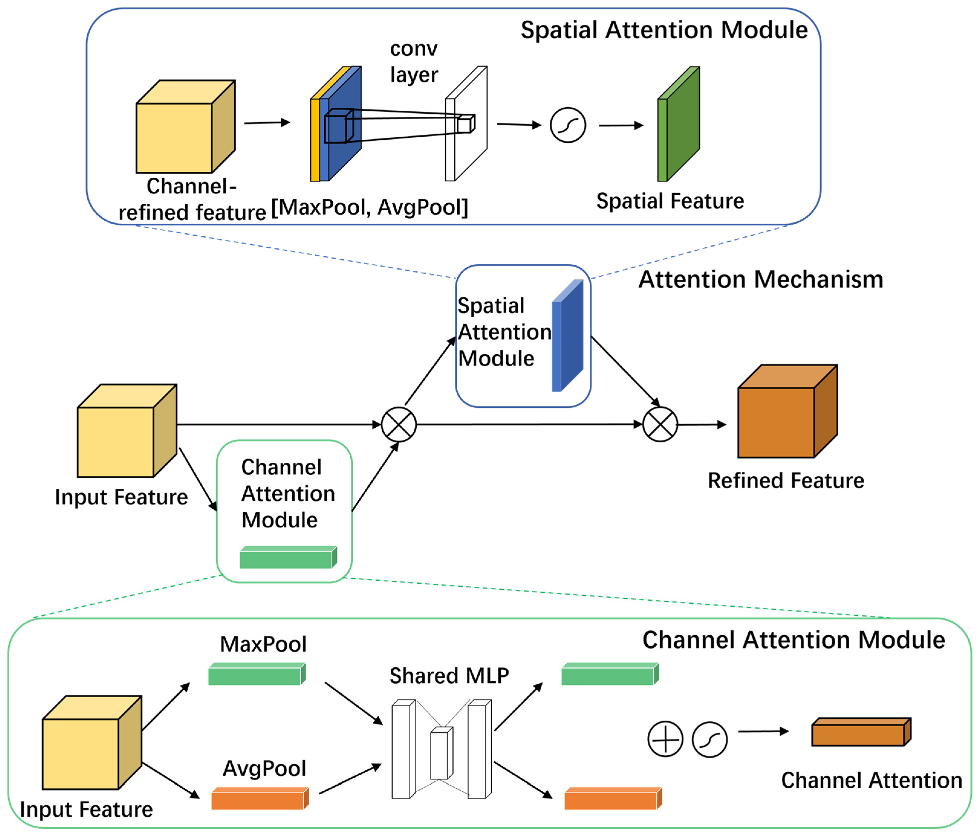
The Convolutional Block Attention Module is an attention mechanism for convolutional neural networks (CNNs) designed to enhance feature representation through channel attention and spatial attention mechanisms. The CBAM module consists of a Channel Attention Module (CAM) and a Spatial Attention Module (SAM), as shown in Figure 3. It allows easy insertion into various positions of the network while being computationally efficient. Compared to attention mechanisms focusing solely on spatial or channel aspects, this approach achieves better results.

The Channel Attention Module, shown in Figure 3, learns dependencies between different channels by computing importance weights for each channel to adjust the response of each channel in the feature map. This helps the network focus on the most important feature channels to enhance feature representation capability. The steps to implement the channel attention module are as follows: For the input feature map, first perform global max pooling and global average pooling operations on each channel to compute the maximum and average feature values per channel. This generates two vectors containing the number of channels, representing the global maximum and average features for each channel. Input the feature vectors from global max pooling and average pooling into a shared fully connected layer. This fully connected layer learns the attention weights for each channel. Through learning, the network can adaptively determine which channels are more important for the current task. Fuse the global maximum feature vector and average feature vector to obtain the final attention weight vector. To ensure attention weights are between 0 and 1, apply the Sigmoid activation function to generate channel attention weights. These weights are then applied to each channel of the original feature map. Multiply the obtained attention weights with each channel of the original feature map to obtain attention-weighted channel feature maps. This emphasizes channels helpful for the current task and suppresses irrelevant channels.

The Spatial Attention Module, shown in Figure 3, focuses on spatial relationships within the feature map by computing importance weights for each spatial position to adjust the spatial distribution of the feature map. This helps the network focus on the most important spatial locations to enhance the spatial representation capability of features. The steps to implement the spatial attention module are as follows: For the input feature map, perform max pooling and average pooling operations along the channel dimension to generate features at different contextual scales. Concatenate the max-pooled and average-pooled features along the channel dimension to obtain a feature map with contextual information at different scales. Then, process this feature map through a convolutional layer to generate spatial attention weights. Similar to the channel attention module, apply the Sigmoid activation function to the generated spatial attention weights to constrain them between 0 and 1. Apply the obtained spatial attention weights to the original feature map, weighting the features at each spatial position. This highlights important image regions and reduces the impact of unimportant regions.

In the present framework, CBAM is used as a feature modulation mechanism rather than as the primary methodological novelty. Its role is to reduce the impact of redundant or noisy fused features, especially when multiple handcrafted descriptors are concatenated and the feature space becomes overloaded.

2.6. Feature Fusion Module

Unlike deep learning methods, which automatically learn hierarchical features from data, traditional handcrafted feature methods construct features based on domain knowledge and understanding of the problem being addressed, which can generate stable and effective features.

First, the five feature maps are resized to the same dimensions, and then the feature weight for each position is calculated:

$$w_i(x,y)={\displaystyle \frac{\exp (f_i(x,y))}{{\displaystyle \sum _{j=1}^5\exp }(f_j(x,y))}}, i\in \{Gradient, DCCR, Canny, HOG, LBP\}$$

(17)

where w_i(x, y) denotes the adaptive fusion weight for the i-th handcrafted feature at pixel coordinate(x, y), satisfying w_i(x, y) ∈ [0, 1] for every spatial location; f_i(x, y) is the saliency measure of the i-th feature map at (x, y), defined as the absolute value of the feature response after local contrast enhancement (i.e., f_i(x, y) = |F_i(x, y)|, where F_i(x, y) is the normalized feature value in the range [0, 1]). Among them, F_DCCR(x, y) is calculated using Formulas (1) to (4). The final fused feature is:

$$F_{\mathrm{fused}}(x,y)={\displaystyle \sum _{i=1}^5{w}_i}(x,y)\cdot F_i(x,y)$$

(18)

where $F_i(x,y)$ denotes the normalized response of the i-th handcrafted feature map prior to fusion; $F_{\mathrm{fused}}(x,y)$ is the resulting fused feature map.

This fusion strategy dynamically adjusts the contribution of each feature based on local scene characteristics.

The aim of the fusion module is not to force all features to contribute equally, but to examine whether structured low-level priors can enrich the detector input. The experimental results later show that some feature combinations are helpful, whereas others may degrade performance, especially in noisy scenes. This finding is important because it suggests that feature fusion in sonar detection should be selective rather than indiscriminate.

3. Results

In this section, we present the side-scan sonar image datasets, experimental parameter settings, evaluation metrics for experimental results, comparison results and analysis of different methods, and algorithm robustness analysis.

3.1. Datasets

Two datasets were used in the experiments in this paper, with a comparison of key attributes between the two datasets shown in

Table 1. Comparison of key attributes between the two datasets.

Attribute	KLSG Dataset	SSS-Bottom Dataset
Scene Complexity	Relatively simple, homogeneous background	High complexity, complex background
Target Characteristics	Targets relatively clear, acoustic shadows obvious	Small targets, blurred edges, low signal-to-noise ratio
Categories	Ships, Aircraft	NOMBO, MILCO
Number of Images	447	240

. The first dataset is the publicly available side-scan sonar image dataset KLSG (https://github.com/huoguanying/SeabedObjects-Ship-and-Airplane-dataset) (accessed on 27 July 2026), and the second dataset is side-scan sonar data collected by the Portuguese Navy’s Third Engineer Diving Team (Destacamento de Mergulhadores Sapadores—DMS 3) in 2015. KLSG contains two categories, ships and aircraft, with a total of 447 images. Among these, there are 395 ship targets and 62 aircraft targets. The second dataset includes two categories, Non-Mine-like Bottom Objects (NOMBO) and Mine-like Contacts (MILCO), with a total of 240 images. Among these, NOMBO appears 175 times and MILCO appears 238 times.

Table 2. The training hyperparameters in the experiment.

Hyperparameter	Value
Optimizer	SGD
Momentum	0.937
Weight Decay	0.0005
Initial Learning Rate (lr0)	0.01
Final Learning Rate (lrf)	0.01
Learning Rate Schedule	linear
Batch Size	4
Input Resolution	640 × 640
Total Epochs	200

is the training hyperparameters in the experiment. The datasets were split into training, validation, and testing sets (70%/10%/20%). The input resolution for all images was uniformly resized to 640 × 640 pixels. The hardware used for model training includes an Intel (R) Core (TM) i5-13500H CPU and an NVIDIA GeForce RTX 4050 GPU with 6G memory. The software compilation environment is PyTorch 2.1.2, CUDA 11.8, and Python 3.11.7 on the Windows 11 system.

3.2. Evaluation Metrics

Three main metrics were used in this study to test the model’s performance. Precision (P) represents the proportion of samples predicted as positive that are actually positive; precision measures the accuracy of the model’s predictions. A higher precision indicates that the model has fewer false positives among the samples it predicts as positive. The calculation formula is shown in (19). Recall (R) refers to the proportion of actual positive samples that are correctly predicted as positive by the model, calculated in (20). Mean Average Precision (mAP@0.5) refers to the average precision (AP) calculated at an Intersection over Union (IoU) threshold of 0.5, and then averaged over all categories, as shown in (21).

$$Precision={\displaystyle \frac{TP}{TP+FP}}$$

(19)

where True Positive (TP) represents correctly classified positive samples, and False Positive (FP) represents incorrectly classified positive samples. TP + FP is the total number of samples predicted as positive.

$$Recall={\displaystyle \frac{TP}{TP+FN}}$$

(20)

In the formula, False Negatives (FN) represents incorrectly classified negative samples; TP + FN is the total number of actual positive samples.

$$mAP0.5={\displaystyle \frac{1}{N}}{\displaystyle \sum _{i=1}^N}{AP}_i (ioU=0.5)$$

(21)

where N is the number of categories, and AP_i is the average precision for the i-th category. mAP@0.5 is one of the most commonly used evaluation metrics in object detection. It comprehensively considers precision and recall and measures the localization accuracy of detection boxes using an IoU threshold of 0.5. A higher mAP@0.5 value indicates better performance of the model in the detection task.

3.3. Ablation Experiments and Analysis

3.3.1. Feature Effectiveness Analysis

To assess the contribution of each handcrafted feature, ablation experiments were conducted on both datasets. The results are reported in

Table 3. Effectiveness Analysis of individual handcrafted features.

Input Feature	Baseline	+Canny	+Grad	+LBP	+HOG	+DCCR (Our)	Δ * vs. Baseline
KLSG	0.935	0.922	0.911	0.911	0.881	0.943	+0.8%
SSS-Bottom	0.855	0.789	0.847	0.748	0.843	0.858	+0.3%

* Note: Values in the table represent mAP@0.5. Values in parentheses indicate the improvement (∆) relative to the baseline.

.

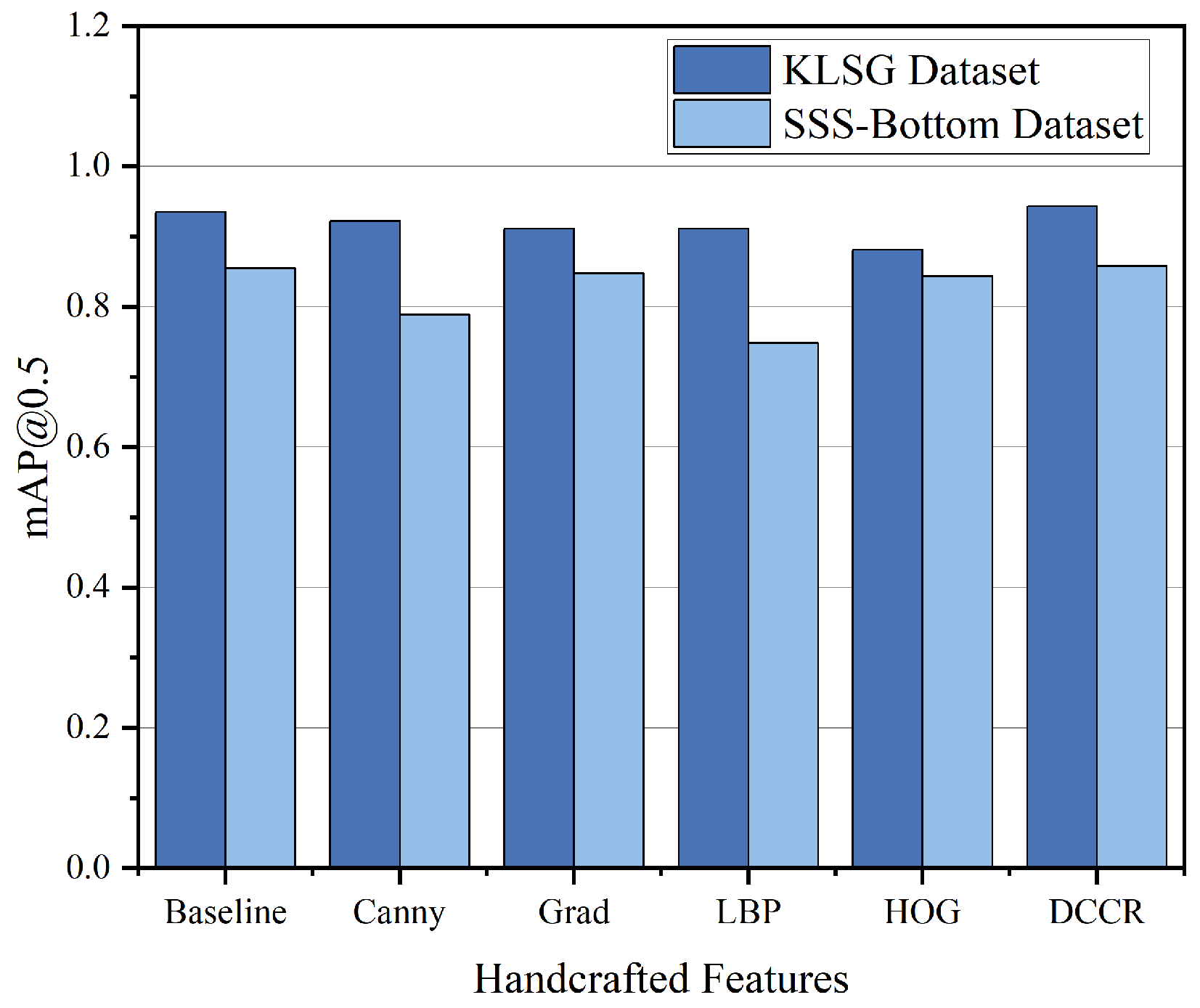
The DCCR feature exhibits the most optimal and stable performance gain. On the KLSG dataset, DCCR improves mAP@0.5 from the baseline of 0.935 to 0.943; on the more complex and noisier SSS-Bottom dataset, DCCR also achieves an improvement from 0.855 to 0.858. Notably, DCCR is the only feature that consistently outperforms the baseline model on both datasets, validating its effectiveness designed for the acoustic characteristics of sonar images and demonstrating good scene adaptability. Additionally, the experiments reveal significant limitations of traditional features in complex underwater scenes. Compared to their performance on the KLSG dataset, features such as Canny and LBP not only failed to improve performance on the SSS-Bottom dataset but actually led to a significant performance decrease. This phenomenon indicates that in sonar images with complex backgrounds and extremely low signal-to-noise ratios, these feature extractors are highly susceptible to noise interference, with the activated edge or texture responses largely originating from background clutter rather than real targets, thereby introducing misleading information to the model.

It can be concluded that proposed DCCR feature is a reliable and effective method for prior knowledge injection. In complex scenarios, feature selection must be prudent, as blindly stacking features may be counterproductive. This provides a direct basis for subsequent exploration of streamlined multi-feature fusion and attention modulation mechanisms.

Figure 4 presents a visual comparison of the detection performance of different input features on the two sonar datasets using a bar chart. Our proposed DCCR feature achieves the highest performance among all handcrafted features on both datasets. On the KLSG dataset (relatively simple scenes), the performance bar for DCCR is significantly higher than other features, validating its ability to extract key acoustic priors. More importantly, on the highly challenging SSS-Bottom dataset (complex, high-noise scenes), although the performance bar for DCCR slightly decreases, the magnitude of the decrease is much smaller than that of all other compared features, and it still maintains an advantage over the baseline.

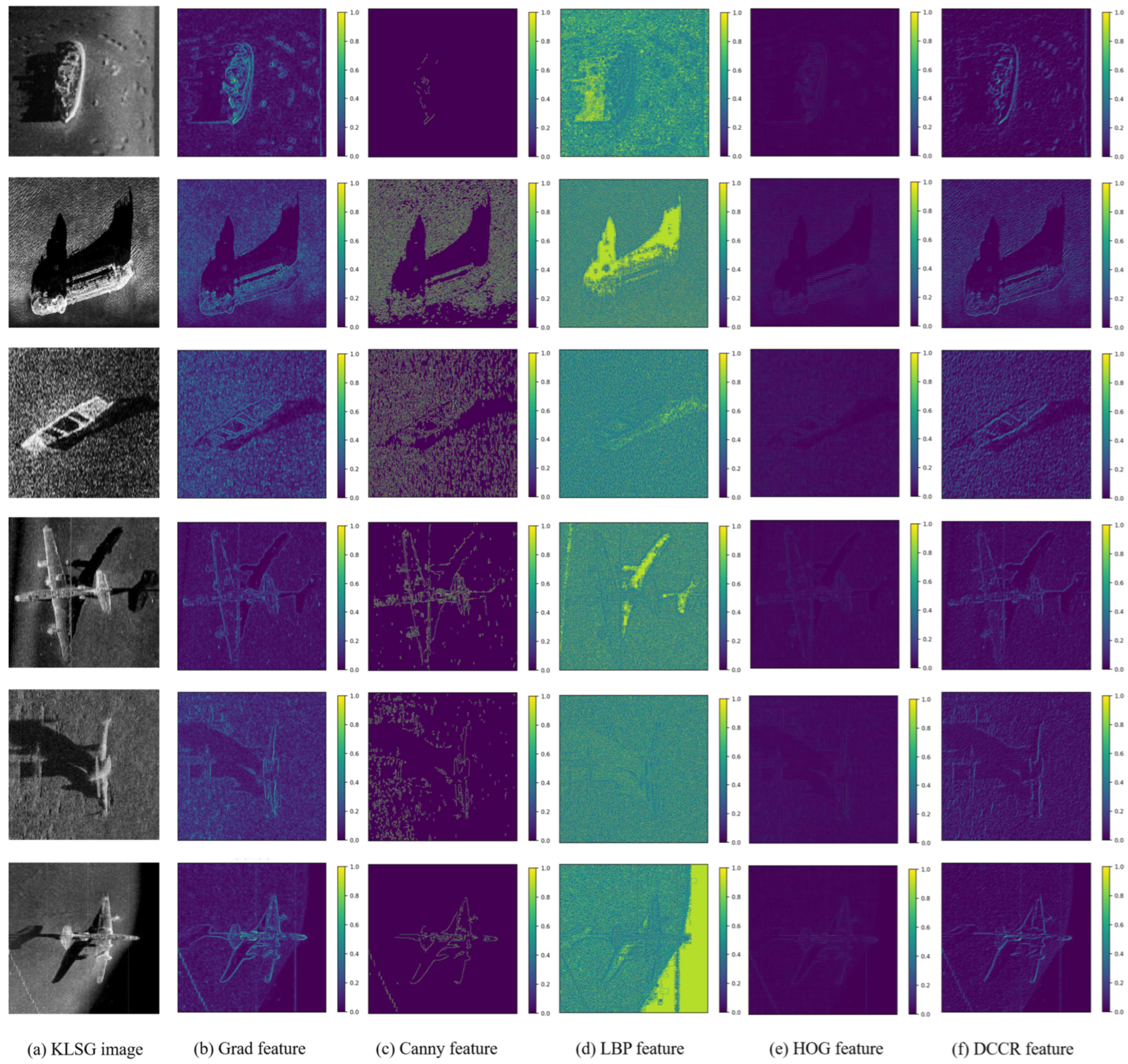
Figure 5 provides an intuitive comparison of the feature responses of different handcrafted features after passing through the network’s first convolutional layer, fully revealing the essential differences in the information captured by each feature in sonar images. The DCCR feature (f) demonstrates a remarkable ability to enhance acoustic characteristics. Compared to the original image (a), the DCCR feature map strengthens the contrast between target regions and acoustic shadow regions while effectively suppressing responses in homogeneous backgrounds. Its response pattern highly aligns with the physical priors of sonar imaging, indicating that DCCR successfully captures the acoustic scattering differences between targets and backgrounds. Traditional edge and texture features are susceptible to background interference. Although the Canny feature (c) clearly extracts edges, the responses are spread throughout the entire image, including a large amount of edge noise from seabed texture and clutter, making it difficult to distinguish targets from backgrounds. LBP feature (d) over-activates texture patterns in the background, causing the target signal to be nearly overwhelmed, which explains its significant performance degradation on complex datasets. While the Grad feature (b) and HOG feature (e) can provide some structural information, their responses lack sufficient discrimination between target regions and background regions.

3.3.2. Analysis of Multi-Feature Fusion Strategies

For different datasets, the impact of different feature combinations on detection performance under various conditions was analyzed separately.

On both datasets, as shown in

Table 4. Impact of various feature combinations on detection performance (KLSG dataset).

Exp. No.	Canny	Grad	LBP	HOG	DCCR (Ours)	mAP@0.5	Change (%)
Baseline	-	-	-	-	-	0.935	-
Best Single Feature					√	0.943	+0.8
Best Dual Feature			√		√	0.906	−2.9
Best Triple Feature	√	√			√	0.927	−0.8
Best Quad Feature	√		√	√	√	0.912	−2.3
Full Fusion	√	√	√	√	√	0.949	+1.4

and

Table 5. Impact of various feature combinations on detection performance (SSS-Bottom dataset).

Exp. No.	Canny	Grad	LBP	HOG	DCCR (Ours)	mAP@0.5	Change (%)
Baseline	-	-	-	-	-	0.855	-
Best Single Feature					√	0.858	+0.3
Best Dual Feature			√		√	0.859	+0.4
Best Triple Feature	√			√	√	0.849	−0.6
Best Quad Feature	√	√		√	√	0.852	−0.3
Full Fusion	√	√	√	√	√	0.808	−4.7

, single-feature combinations including DCCR outperformed the baseline. Notably, on the SSS-Bottom dataset, only multi-feature combinations containing DCCR achieved performance improvements, while all other combinations led to performance degradation. This again confirms the value of DCCR as core prior information. On the KLSG dataset, the table data shows that full feature fusion achieved an mAP@0.5 of 0.949, a 1.4% improvement over the baseline. It is worth noting that certain feature combinations produced significant negative synergy. On the KLSG dataset, the performance of DCCR + LBP was even lower than using the single DCCR feature; on SSS-Bottom, the performance of full fusion dropped sharply. This indicates that some feature combinations not only fail to complement each other but also interfere with one another, especially in complex scenes.

This set of experiments not only validates the potential value of feature fusion but also reveals its limitations in complex scenarios. It indicates that the benefit of early fusion depends on the relevance and compatibility of the selected features. In complex sonar scenes, simply increasing the number of input features does not guarantee better results. Instead, feature selection should consider whether the descriptor captures useful target information or mostly introduces redundant noise.

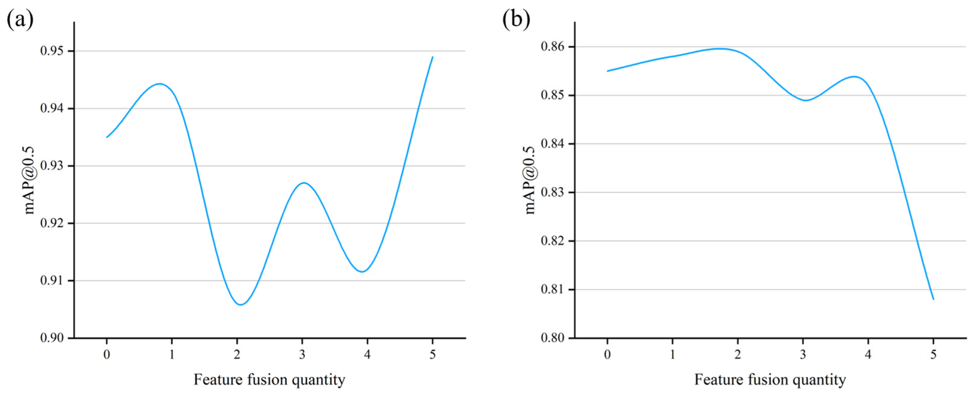
As shown in Figure 6a, on the KLSG dataset (simple scenes), model performance generally shows a fluctuating upward trend as the number of fused features increases. Full feature fusion achieved the best mAP@0.5 of 0.949, a 1.4% improvement over the baseline. This validates that in high signal-to-noise ratio scenes, the complementary information provided by multiple features can be effectively utilized by the model.

However, on the SSS-Bottom dataset (complex scenes), the situation is completely opposite. Figure 6b shows that as the number of features increases, performance generally trends downward, with full feature fusion performing 4.7% lower than the baseline. In complex, high-noise underwater environments, blindly stacking features injects a large amount of background noise patterns into the network, causing the model to become overloaded and unable to focus on true target signals.

3.3.3. Analysis of Attention Mechanism Effects

To investigate whether attention modulation can mitigate the negative effects of feature redundancy, experiments were conducted on both datasets by setting conditions with and without the attention mechanism, under different fusion scenarios including single feature, dual feature, triple feature, and full feature fusion, as shown in

Table 6. Effect of attention mechanism on mAP@0.5 for different fusion configurations on both datasets.

Feature Configuration	With CBAM (mAP@0.5)	Without CBAM (mAP@0.5)
KLSG Dataset
Baseline	0.930	0.935
Single-Feature Fusion
Canny	0.906	0.922
Grad	0.865	0.911
DCCR	0.896	0.943
Dual-Feature Fusion
Canny + Grad	0.899	0.876
Canny + DCCR	0.931	0.902
Grad + DCCR	0.916	0.905
Triple-Feature Fusion
Canny + DCCR + Grad	0.914	0.927
Full-Feature Fusion
Canny + Grad + DCCR + HOG + LBP	0.887	0.949
SSS-Bottom Dataset
Baseline	0.849	0.855
Single-Feature Fusion
DCCR	0.849	0.828
Dual-Feature Fusion
Canny + DCCR	0.834	0.759
Canny + Grad	0.839	0.829
Grad + DCCR	0.866	0.801
Full-Feature Fusion
Canny + Grad + DCCR + HOG + LBP	0.844	0.808

.

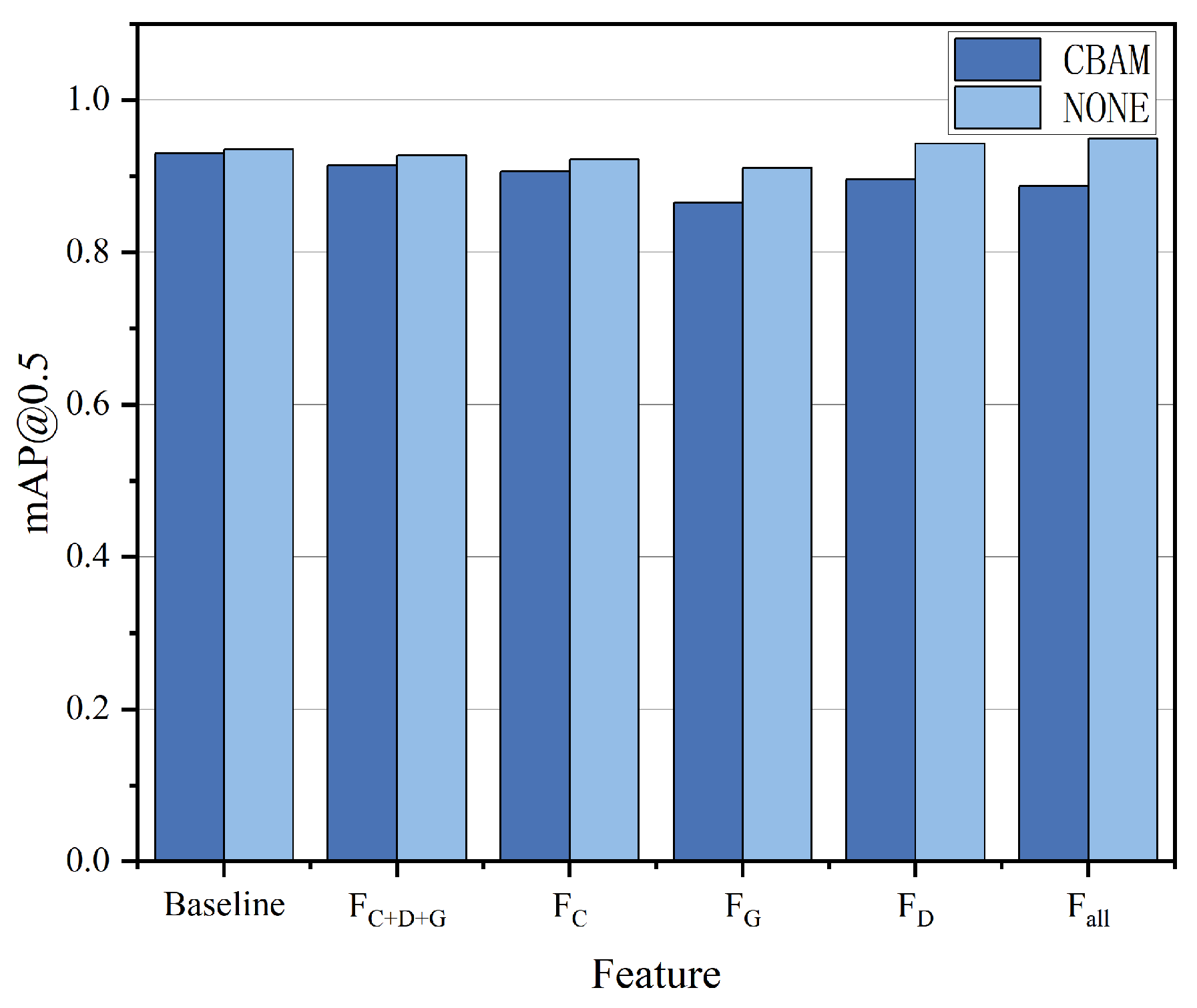
On the relatively simple KLSG dataset, a core and counterintuitive trend is that for the vast majority of feature combinations, adding CBAM actually decreases performance. This is particularly evident in two key cases. For the single feature DCCR, performance without CBAM is as high as 0.943, but drops to 0.896 after adding it. For full feature fusion, the best performance of 0.949 is achieved without CBAM, but it drops significantly to 0.887 after adding it. In simple scenes like KLSG with clean backgrounds and clear targets, high-quality features (especially DCCR) or effective feature combinations themselves already provide a very high signal-to-noise ratio input. At this point, adding an extra attention module may become redundant, or even interfere with the originally clear feature representation due to unnecessary parameterization and nonlinear transformations, leading to over-design and performance loss.

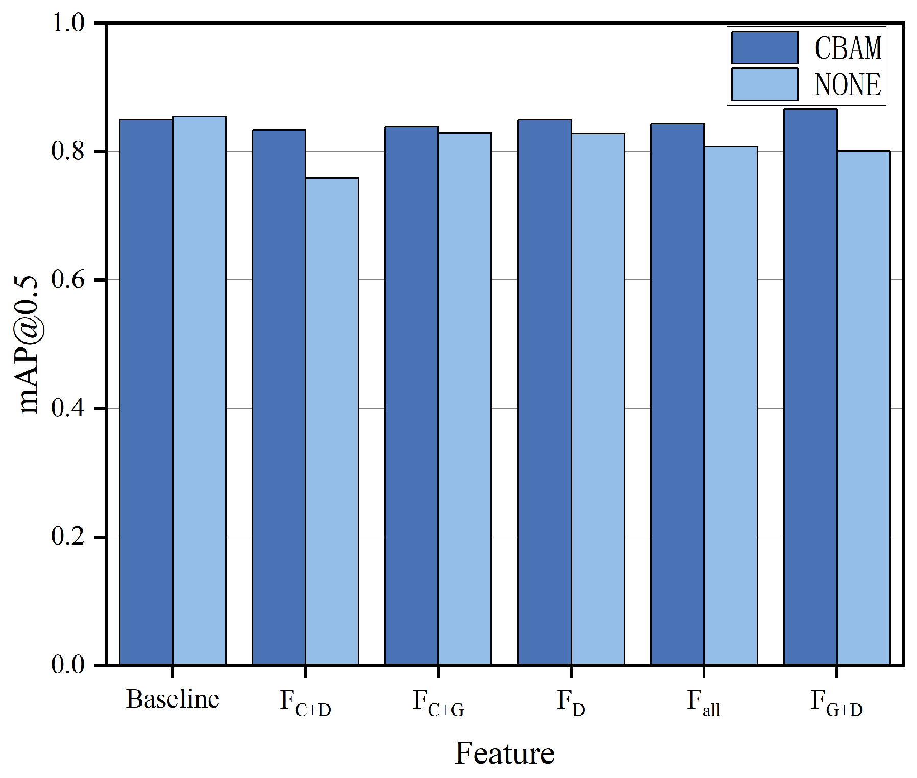
On the SSS-Bottom dataset, the table clearly reveals the key modulatory role and applicable scenarios of the attention module in complex sonar target detection. CBAM can significantly optimize effective feature combinations. For the strong feature combination Grad + DCCR, adding CBAM brings a performance improvement. This indicates that when the input itself contains high-quality prior information, CBAM can adaptively suppress redundancy and focus on key elements through channel and spatial attention mechanisms, thereby maximizing feature efficacy. However, for the baseline with lower information density, introducing CBAM instead causes a slight performance decrease, from 0.855 to 0.849, indicating that the attention mechanism cannot leverage its advantages when lacking effective input. In the case of full feature fusion (Canny + Grad + DCCR + HOG + LBP), model performance is lowest without CBAM, consistent with the earlier finding that feature stacking in complex scenes introduces noise. After adding CBAM, performance significantly recovers to 0.844. The visualization results indicate that handcrafted features and CBAM may help the detector focus on target-relevant regions. This experiment strongly validates that, in a network based on early fusion, the attention mechanism is not always beneficial, but its modulatory role on high-quality feature combinations in complex scenes is crucial. Performing early fusion with core features like DCCR + Grad, supplemented by late modulation with CBAM.

As shown in Figure 7, in the simple KLSG scene, introducing the attention mechanism did not bring gains in most cases, and even led to performance degradation. The most striking will be the two sets of data corresponding to full feature fusion and the single feature DCCR. The chart shows that under these two configurations, the bars representing the condition without CBAM will be significantly higher than those with CBAM. This visually striking reversal strongly proves that in simple scenes where the feature information itself is already sufficiently high-quality and clear, an additional attention module can become a source of interference.

As shown in Figure 8, the bar chart intuitively displays the effect of the attention mechanism on different feature combinations, visually reinforcing the following key findings. The analysis of full feature fusion demonstrates that the model exhibits significantly degraded performance without the attention mechanism, a phenomenon attributable to performance collapse caused by feature stacking in complex underwater environments. After introducing the attention mechanism, the bar height significantly recovers, clearly demonstrating the module’s effectiveness as a feature filter, capable of suppressing redundant noise and improving information utilization. The bar chart highlights the optimal feature combination, where the height difference for the Grad + DCCR combination is most prominent. Without the attention mechanism, this combination already has a certain performance foundation; after introducing the attention mechanism, its bar height rises substantially, reaching the peak among all configurations. This intuitively confirms that the attention mechanism can precisely modulate high-quality feature combinations, achieving further performance breakthroughs.

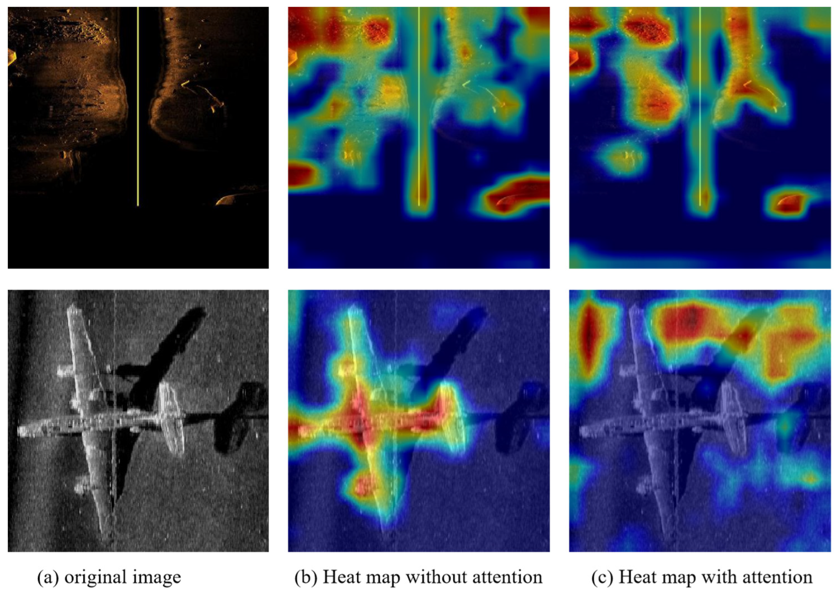
To further understand how CBAM improves detection performance, we visualize the attention weights of the CBAM module in Figure 9. In the complex SSS-Bottom scene, the attention maps exhibit high responses around the target echo and its associated acoustic shadow. This confirms that the attention mechanism plays a crucial role in suppressing feature redundancy and guiding the network to focus on sonar-relevant structures. On the relatively simple KLSG dataset, for the vast majority of feature combinations, adding CBAM actually decreases performance. In simple scenes like KLSG, the high input SNR provides clear features, making attention modules redundant. Their unnecessary non-linear transformations may interfere with representation, leading to performance loss.

This observation is important because it shows that attention should not be treated as a universally beneficial plug-in module. Its value depends on the extent to which the fused features still contain structured but noisy responses that can be selectively refined. In other words, attention is most helpful when the input features are informative but not yet well organized. For unknown scenarios, it is recommended to adopt the robust configuration of DCCR + Grad + CBAM, which is called MFEF-Det-S. If the scene is known to be simple, then the DCCR features without CBAM can be selected to pursue the ultimate performance, which is called MFEF-Det-K.

4. Discussion

4.1. Advantages of the Proposed Method

(1)

Synergistic Enhancement of Domain Prior Knowledge and Deep Representation Capabilities. Unlike pure data-driven end-to-end learning methods, this network explicitly injects traditional features with clear physical meanings and DCCR features designed for the imaging characteristics of side-scan sonar into the input end of the network. Through this early fusion strategy, the model is relieved from learning low-level foundational features such as edges and textures from scratch, thereby allowing its limited learning capacity to focus on higher-order semantic modeling. Ablation experiments demonstrate that even the single-feature DCCR alone yields stable performance improvements on both datasets, directly validating the positive value of domain prior knowledge.

(2)

Adaptive Robustness Oriented towards Scene Complexity. In the relatively simple KLSG dataset, the DCCR feature alone can be selected to pursue optimal performance, whereas in the highly complex SSS-Bottom dataset, the combination of a streamlined feature set together with the attention mechanism constitutes the optimal configuration. This disparity precisely reflects the flexibility of the proposed network. Users can flexibly configure the feature combination and the activation status of the attention mechanism according to the noise level and target characteristics of the actual application scenario.

(3)

Substantial Enhancement of Model Interpretability. Due to black-box nature, traditional deep learning models face challenges in tracing the decision-making process and may learn spurious correlations. By introducing traditional features with clear physical meaning, this network endows the model’s input information with an analyzable semantic foundation. Feature map visualizations reveal that DCCR feature responses exhibit a high degree of consistency with target acoustic shadow regions. When the model produces erroneous predictions, the cause can be identified by tracing the activation states of individual feature input channels or attention weights, thereby significantly enhancing the model’s credibility.

4.2. Comparison with Existing Methods

To examine the performance of the MFEF-Det network, experimental testing and quantitative analysis were performed on two datasets, and the results were benchmarked against those of classical methods. This section provides the comparative results for each model, with the quantitative evaluation metrics listed in the tables.

To ensure a fair and unbiased comparison, all competing methods were trained from scratch under a strictly unified training protocol. The complete set of hyperparameters is provided in Table 2. To account for the inherent randomness in deep learning training, all reported results are averaged over three independent trials with different random seeds. The standard deviation is also provided to assess the statistical stability of each method.

Table 7. Quantitative Evaluation of Experimental Results on the KLSG Dataset. All results are reported as mean ± standard deviation over three independent runs with different random seeds.

Model	Input Shape	Precision	Recall	F1	mAP@0.5
YOLOv5	640 × 640	0.852 ± 0.034	0.848 ± 0.031	0.850 ± 0.023	0.908 ± 0.020
YOLOv8	640 × 640	0.810 ± 0.118	0.748 ± 0.082	0.770 ± 0.046	0.840 ± 0.008
YOLOv9	640 × 640	0.733 ± 0.086	0.706 ± 0.052	0.715 ± 0.027	0.795 ± 0.008
YOLOv10	640 × 640	0.707 ± 0.086	0.585 ± 0.066	0.636 ± 0.032	0.689 ± 0.036
YOLOv11	640 × 640	0.890 ± 0.046	0.842 ± 0.034	0.865 ± 0.021	0.898 ± 0.030
L-FFCA-YOLO [27]	640 × 640	0.773 ± 0.075	0.732 ± 0.171	0.749 ± 0.117	0.791 ± 0.138
MFEF-Det-K	640 × 640	0.914 ± 0.036	0.887 ± 0.020	0.900 ± 0.022	0.933 ± 0.016

and

Table 8. Quantitative Evaluation of Experimental Results on the SSS-Bottom Dataset. All results are reported as mean ± standard deviation over three independent runs with different random seeds.

Model	Input Shape	Precision	Recall	F1	mAP@0.5
YOLOv5	640 × 640	0.758 ± 0.049	0.762 ± 0.082	0.760 ± 0.065	0.777 ± 0.071
YOLOv8	640 × 640	0.631 ± 0.095	0.530 ± 0.076	0.569 ± 0.035	0.583 ± 0.051
YOLOv9	640 × 640	0.604 ± 0.071	0.493 ± 0.024	0.541 ± 0.029	0.530 ± 0.022
YOLOv10	640 × 640	0.609 ± 0.184	0.537 ± 0.099	0.571 ± 0.098	0.541 ± 0.134
YOLOv11	640 × 640	0.710 ± 0.172	0.545 ± 0.080	0.602 ± 0.042	0.603 ± 0.040
L-FFCA-YOLO	640 × 640	0.696 ± 0.071	0.719 ± 0.094	0.701 ± 0.016	0.751 ± 0.038
MFEF-Det-S	640 × 640	0.833 ± 0.058	0.821 ± 0.065	0.827 ± 0.057	0.866 ± 0.052

comprehensively compare the performance of proposed method with multiple advanced baseline models on the KLSG and SSS-Bottom datasets. A comprehensive set of evaluation metrics, including precision, recall, F1-score, and mAP@0.5, is adopted to comprehensively validate the effectiveness, computational efficiency, and competitive stability of the presented multi-stream early feature fusion network with attentional modulation modules.

On the relatively simple KLSG dataset, MFEF-Det-K achieved competitive detection performance. In terms of detection accuracy, the proposed method achieves an mAP@0.5 of 0.933 ± 0.016, which delivers consistent performance improvements over other methods. This phenomenon indicates that the introduction of the customized acoustic feature DCCR can support competitive model accuracy under low computational consumption, which verifies the efficacy of embedding high-quality domain prior knowledge for detection optimization.

On the challenging SSS-Bottom dataset with complex backgrounds and blurred target features, the superiority of the proposed method is further reflected. MFEF-Det-S obtains optimal overall performance among all comparison methods, reaching an mAP@0.5 of 0.866 ± 0.052, an F1-score of 0.827 ± 0.057. Compared with L-FFCA-YOLO and other mainstream YOLO variants including YOLOv5, YOLOv8, YOLOv9, YOLOv10, and YOLOv11, the proposed method yields consistent performance gains across core detection metrics and shows certain stability in complex noisy scenarios. These results validate the necessity of multi-feature complementary fusion and attention modulation mechanisms for complex scene detection. In harsh environments with high background noise and indistinct target features, the single DCCR feature can hardly meet the detection requirements. The fusion of gradient information and dynamic feature enhancement via attention mechanisms is capable of facilitating steady metric optimization, enabling the model to maintain certain stability under complex interference conditions.

In summary, cross-dataset evaluation shows that on both datasets, models based on DCCR significantly outperform the original baseline, proving its effectiveness as a carrier of acoustic prior knowledge. The network possesses scene adaptation capability.

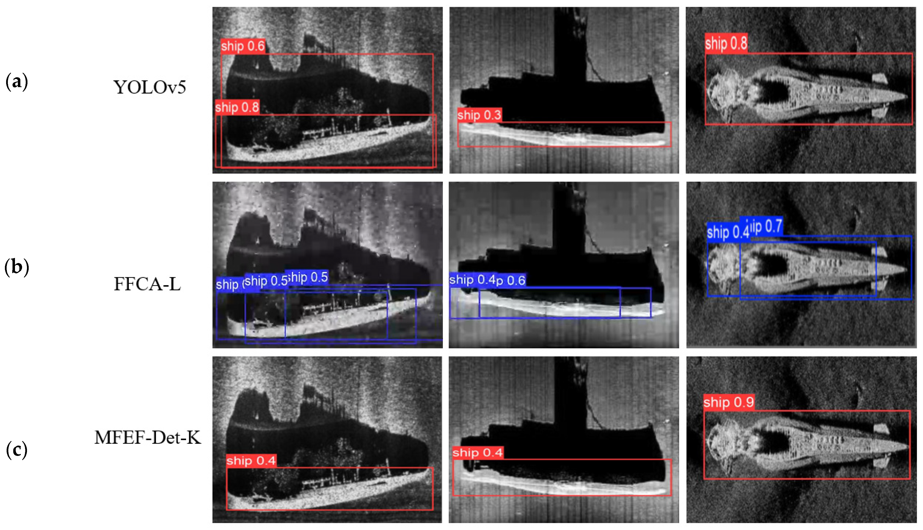
Figure 10 intuitively demonstrates the target detection performance of YOLOv5, L-FFCA-YOLO, and the proposed MFEF-Det-K network on the same side-scan sonar scene. By comparing the positions and confidence scores of the detection boxes, the significant advantages of our method are clearly visible. In terms of target positioning, although YOLOv5 can detect some ship targets, the confidence level of its detection boxes is relatively low, and the positions of the detection boxes are inaccurate. The L-FFCA-YOLO model produces duplicate bounding boxes for the same target, indicating that this model still faces challenges when dealing with low-contrast targets. In contrast, the proposed MFEF-Det-K network demonstrates optimal detection performance. Its detection boxes accurately cover the target areas, and the confidence scores are significantly improved.

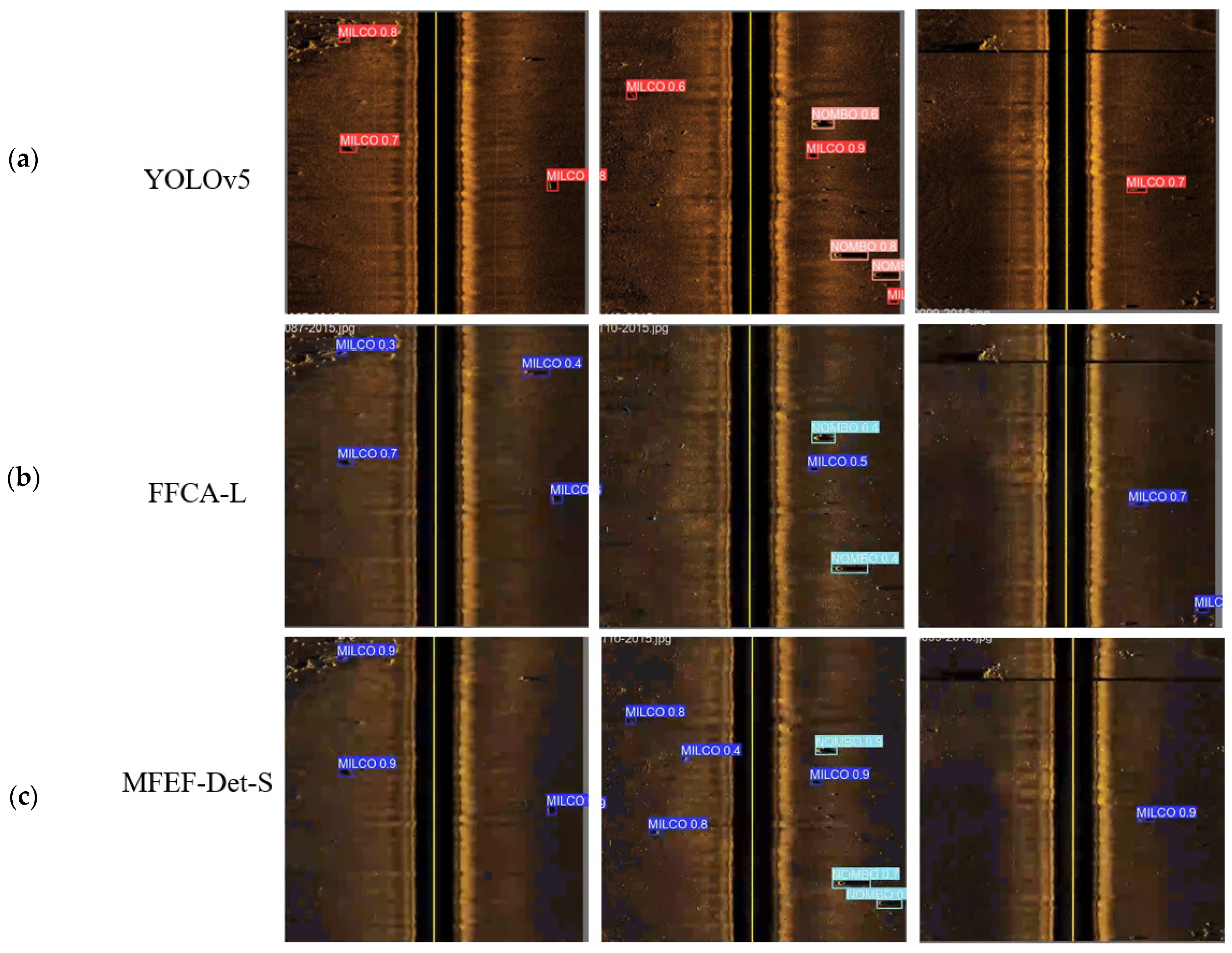
Figure 11 presents representative qualitative results on challenging SSS-Bottom samples with complex backgrounds and relatively low signal-to-noise ratios. In these examples, the detection results of YOLOv5 show that although the model can locate some targets, the confidence scores are generally low, indicating that the baseline model’s discriminative ability degrades significantly under complex backgrounds, making it susceptible to interference from seabed textures, reverberation, and other noise. The detection results of L-FFCA-YOLO are improved compared to YOLOv5, but still exhibit obvious confidence degradation, suggesting that this model remains insufficient for effectively suppressing background clutter in complex environments. In contrast, MFEF-Det-S provides more accurate localization and higher confidence for real targets than YOLOv5 and L-FFCA-YOLO. Nevertheless, these representative examples do not imply that MFEF-Det-S achieves ideal detection performance. The model may still fail when target highlights and acoustic shadows are extremely weak or visually similar to strong seabed textures.

The comprehensive performance evaluation quantitatively assesses the proposed method, which incorporates domain-specific prior feature-guided early fusion and complexity-oriented attention modulation. A target detector for side-scan sonar images is constructed, and the approach is examined as a potential solution for target detection challenges in complex underwater environments.

4.3. Effect of Input Shape on the Detection Results

It is also worth discussing the universality of the proposed framework with respect to input resolution. While all experiments adopt the standard 640 × 640 input size to ensure a fair comparison with existing YOLO-based methods, the proposed early-fusion architecture is not inherently tied to a fixed resolution. To validate this, we additionally evaluated the baseline and our MFEF-Det under two alternative input scales: 512 × 512 and 800 × 800, without modifying any network components or retuning hyperparameters.

As shown in

Table 9. Input shape generalization analysis of the proposed method versus the baseline.

Dataset	Input Size	Baseline (mAP@0.5)	MFEF-Det (mAP@0.5)
KLSG	512 × 512	0.883	0.886
	640 × 640	0.935	0.943
	800 × 800	0.858	0.928
SSS-Bottom	512 × 512	0.781	0.835
	640 × 640	0.855	0.866
	800 × 800	0.816	0.947

, our method consistently outperforms YOLOv5 across all tested resolutions, with mAP@0.5 improvements of 0.3% and 7.0% on KLSG, and 5.4% and 13.1% on SSS-Bottom, respectively. This confirms that the performance gains achieved by our domain-specific feature fusion are robust to input scale variations. Notably, under the higher input resolution (800 × 800) on the challenging SSS-Bottom dataset, our method achieves a substantial gain of 13.1%. This observation suggests that handcrafted features, including the DCCR and HOG descriptors, derive greater benefit from increased spatial resolution compared with the purely data-driven baseline, since they explicitly encode local structural information that exhibits enhanced discriminability at finer scales.

4.4. Effect of Fusion Strategies on the Detection Results

To further validate the effectiveness of the proposed early fusion strategy, we compared it against one alternative configuration. Feature sum fusion, where the five normalized handcrafted feature maps are first aggregated via pixel-wise summation into a single channel, which is then concatenated with the raw image.

As reported in

Table 10. Comparison of different feature fusion strategies.

Fusion Strategy	mAP@0.5
Feature sum fusion	0.827
Early fusion(ours)	0.866

, the proposed early channel-wise concatenation achieves an mAP@0.5 of 0.866, substantially outperforming the sum fusion strategy. Unlike sum fusion, which forces heterogeneous features into a single additive representation with ambiguous physical meaning, channel-wise concatenation maintains the distinct identity of each feature, allowing the subsequent convolutional layers to adaptively learn their relative contributions without mutual interference. These results confirm that early fusion is a more effective and interpretable fusion mechanism for integrating handcrafted features in sonar target detection.

4.5. Limitations of the Proposed Method

(1)

Computational Overhead in the Preprocessing Stage. In the feature extraction stage, it is necessary to compute five types of features in parallel: Canny, Grad, LBP, HOG, and DCCR. This introduces additional preprocessing time. Although this overhead can be mitigated through GPU parallelization strategies, it may still become a performance bottleneck in scenarios with extremely stringent real-time requirements. Future work will explore embedding the generation process of physical features like DCCR into the network in the form of differentiable modules, enabling end-to-end joint optimization.

(2)

Performance Degradation under Extremely Low Signal-to-Noise Ratio Conditions. When the target signal is completely submerged in strong reverberation or background noise, all features struggle to extract effective target-related information. Under such extreme conditions, the detection performance of the proposed method degrades significantly. Future work should incorporate temporal information or multi-frame joint processing mechanisms to compensate for this limitation.

4.6. Practical Applicability and Engineering Prospects

(1)

General Potential for Cross-Task Transferability. The methodology proposed in this network is not only applicable to side-scan sonar target detection but can also be extended to other remote sensing image interpretation tasks characterized by low signal-to-noise ratios and small targets, such as ship detection in synthetic aperture radar (SAR) imagery and target recognition in ground-penetrating radar. Furthermore, the design principles of the DCCR feature can be re-customized according to the physical imaging characteristics of different sensors, thereby expanding the application boundaries of this network.

(2)

Support for Human–Machine Collaborative Decision-Making. By incorporating traditional features with clear physical significance, this network enables operators to quickly understand the basis of the model’s detections through visualized feature maps. In tasks such as underwater unidentified object identification and mine detection, this interpretability helps establish human–machine trust and provides experts with auxiliary judgmental evidence, thereby enhancing the reliability and safety of overall decision-making.

5. Conclusions

This study investigated a multi-feature early fusion network for side-scan sonar target detection. The core idea of this network is to explicitly and early fuse the physical prior knowledge of acoustic imaging with the powerful representation capabilities of deep learning, thereby guiding the network to learn the essential characteristics of targets more efficiently. Through systematic experiments and analysis, this study draws the following main conclusions: The proposed DCCR feature is an effective acoustic prior representation. Designed specifically for the directional contrast characteristics of sonar shadows and echoes, it demonstrates stable performance gains on two distinctly different datasets, KLSG and SSS-Bottom, proving the feasibility of converting domain knowledge into structured feature input. The early fusion architecture is a key bridge connecting traditional features and deep learning. Experiments show that channel-wise concatenation of raw images and multiple handcrafted features at the input of the backbone network provides richer and more discriminative information for the model, yielding gains superior to baseline models using only raw data, especially for small targets and complex backgrounds. The role of the attention mechanism is scene-dependent and is key to improving robustness in complex scenes. On the simple KLSG dataset, clear feature fusion is sufficient. While on the high-noise SSS-Bottom dataset, the attention mechanism effectively suppresses feature redundancy and background interference. This difference precisely demonstrates the intrinsic ability of this network to intelligently adapt to different scenes. Comprehensive performance validates the superiority of the model. Comparisons with YOLOv5, YOLOv8, YOLOv9,YOLOv10,YOLOv11, and L-FFCA-YOLO show that this method achieves improvements in detection accuracy, with particularly clear advantages in the most challenging complex seabed scenes.

References

1. Yang, Z.; Zhao, J.; Zhao, X.; Huang, C. Feature super-resolution-based method for small-scale target detection and segmentation in side-scan sonar. Eng. Appl. Artif. Intell. 2025, 161, 112235. [Google Scholar] [CrossRef] [Scilit]
2. Yu, Y.; Zhao, J.; Gong, Q.; Huang, C.; Zheng, G.; Ma, J. Real-time underwater maritime object detection in side-scan sonar images based on transformer-YOLOv5. Remote Sens. 2021, 13, 3555. [Google Scholar] [CrossRef] [Scilit]
3. Cao, Y.; Liu, G.; Mu, L.; Zeng, Z.; Zhao, E.; Xing, C. Sonar image target detection based on multi-region optimal selection strategy. J. Northwest. Polytech. Univ. 2023, 41, 153–159. [Google Scholar] [CrossRef] [Scilit]
4. Fakiris, E.; Papatheodorou, G.; Geraga, M.; Ferentinos, G. An Automatic Target Detection Algorithm for Swath Sonar Backscatter Imagery, Using Image Texture and Independent Component Analysis. Remote Sens. 2016, 8, 373. [Google Scholar] [CrossRef] [Scilit]
5. Yang, F.; Du, Z.; Wu, Z.; Li, J.; Chu, F. Object Recognizing on Sonar Image Based on Histogram and Geometric Feature. Mar. Sci. Bull. 2006, 25, 64. [Google Scholar]
6. Gao, C.C.; Hui, X.W. GLCM-based texture feature extraction. Comput. Syst. Appl. 2010, 19, 195–198. [Google Scholar]
7. Guo, J.; Ma, J.-F.; Wang, A.X. Study of side scan sonar image classification based on SVM and gray level co-occurrence matrix. Geomat. Spat. Inf. Technol. 2015, 68, 60–63. [Google Scholar]
8. Bian, H.; Chen, Y.; Zhang, Z.; Jiang, H. Target detection algorithm inside-scan sonar image based on pixel importance measurement. Acta Acust. 2019, 44, 353–359. [Google Scholar]
9. Dong, L.Y.; Shan, R.; Liu, H.; Yu, D.; Du, K. Shipwreck identification with side scan sonar image based on fractal texture. Mar. Geol. Quat. Geol. 2021, 41, 232–239. [Google Scholar]
10. Tang, Y.; Wang, L.; Bian, S.; Jin, S.; Dong, Y.; Li, H.; Ji, B. SSS underwater target image samples augmentation based on the cross-domain mapping relationship of images of the same physical object. IEEE J. Sel. Top. Appl. Earth Obs. Remote Sens. 2023, 16, 6393–6410. [Google Scholar] [CrossRef] [Scilit]
11. Shi, P.; He, Q.; Zhu, S.; Li, X.; Fan, X.; Xin, Y. Multi-scale fusion and efficient feature extraction for enhanced sonar image object detection. Expert Syst. Appl. 2024, 256, 124958. [Google Scholar] [CrossRef] [Scilit]
12. Li, S.D.; Wang, X.; Zhang, B.Y.; Qin, P.Q.; Dai, Z.Q. Research on shipwreck detection method from side-scan sonar image based on improved YOLOX. Hydrogr. Surv. Chart. 2022, 42, 32–36. [Google Scholar]
13. Tang, Y.; Li, H.; Zhang, W.; Bian, S.; Zhai, G.; Liu, M.; Zhang, X. Lightweight DETR-YOLO method for detecting shipwreck target in side scan sonar. Syst. Eng. Electron. 2022, 44, 2427–2436. [Google Scholar]
14. Zhang, Z.; Shuai, C.; Yuan, C.; Li, B.; Ma, J.; Shang, X. ESL-YOLO: Edge-Aware Side-Scan Sonar Object Detection with Adaptive Quality Assessment. J. Mar. Sci. Eng. 2025, 13, 1477. [Google Scholar] [CrossRef] [Scilit]
15. Cui, X.; Zhang, J.; Zhang, L.; Zhang, Q.; Han, J. Small object detection in side-scan sonar images based on SOCA-YOLO and image restoration. Front. Mar. Sci. 2025, 12, 1542832. [Google Scholar] [CrossRef] [Scilit]
16. Wang, Z.; Zhang, S.; Zhang, C.; Wang, B. RPFNet: Recurrent pyramid frequency feature fusion network for instance segmentation in side-scan sonar images. IEEE J. Sel. Top. Appl. Earth Obs. Remote Sens. 2023, 1–17. [Google Scholar] [CrossRef] [Scilit]
17. Lin, Y.; Song, L.; Feng, Q.; He, S.; Huang, N.; Zhu, Y. DFSE-YOLO: Deep feature selective enhancement for efficient shipwreck detection in side-scan sonar imagery. Sci. Rep. 2026, 16, 3227. [Google Scholar] [CrossRef] [Scilit] [PubMed]
18. Yang, N.; Li, G.; Wang, S.; Wei, Z.; Ren, H.; Zhang, X.; Pei, Y. SS-YOLO: A Lightweight Deep Learning Model Focused on Side-Scan Sonar Target Detection. J. Mar. Sci. Eng. 2025, 13, 66. [Google Scholar] [CrossRef] [Scilit]
19. Hassan, E.; Khalil, Y.; Ahmad, I. Learning Feature Fusion in Deep Learning-Based Object Detector. J. Eng. 2020, 2020, 7286187. [Google Scholar] [CrossRef] [Scilit]
20. Ran, Q.; Wang, Q.; Zhao, B.; Wu, Y.; Pu, S.; Li, Z. Lightweight oriented object detection using multiscale context and enhanced channel attention in remote sensing images. IEEE J. Sel. Top. Appl. Earth Obs. Remote Sens. 2021, 14, 5786–5795. [Google Scholar] [CrossRef] [Scilit]
21. Li, F.; Feng, R.; Han, W.; Wang, L. An augmentation attention mechanism for high-spatial-resolution remote sensing image scene classification. IEEE J. Sel. Top. Appl. Earth Obs. Remote Sens. 2020, 13, 3862–3878. [Google Scholar] [CrossRef] [Scilit]
22. Liu, Q.; Ye, Z.; Zhu, C.; Ouyang, D.; Gu, D.; Wang, H. Intelligent Target Detection in Synthetic Aperture Radar Images Based on Multi-Level Fusion. Remote Sens. 2025, 17, 112. [Google Scholar] [CrossRef] [Scilit]
23. Wang, C.; Lu, W.; Li, X.; Yang, J.; Luo, L. M4-SAR: A Multi-Resolution, Multi-Polarization, Multi-Scene, Multi-Source Dataset and Benchmark for Optical-SAR Fusion Object Detection. arXiv 2025, arXiv:2505.10931. [Google Scholar]
24. Yu, L.; Zhi, X.; Zhang, S.; Jiang, S.; Hu, J.; Zhang, W.; Huang, Y. A Method for Detecting Aircraft Small Targets in Remote Sensing Images by Using CNNs Fused With Handcrafted Features. IEEE Geosci. Remote Sens. Lett. 2024, 21, 6010105. [Google Scholar] [CrossRef] [Scilit]
25. Alakhtar, R.; Alsobhi, H.; Khawaja, A.; Alkhudhayr, H.; Binyamin, S.S.; Ragab, M. Intelligent underwater mine detection using multi-backbone feature fusion with temporal attention-gated unit on side-scan sonar imaging. Sci. Rep. 2026, 16, 21669. [Google Scholar] [CrossRef] [Scilit] [PubMed]
26. Zhu, J.; Li, H.; Qing, P.; Hou, J.; Peng, Y. Side-Scan Sonar Image Augmentation Method Based on CC-WGAN. Appl. Sci. 2024, 14, 8031. [Google Scholar] [CrossRef] [Scilit]
27. Zhang, Y.; Ye, M.; Zhu, G.; Liu, Y.; Guo, P.; Yan, J. FFCA-YOLO for small object detection in remote sensing images. IEEE Trans. Geosci. Remote Sens. 2024, 62, 5611215. [Google Scholar] [CrossRef] [Scilit]
Figure 1. Conceptual illustration of two design paradigms: internal modifications to deep learning backbones (left) versus fusion with interpretable traditional features (right).
Applsci 16 07683 g001
Figure 2. Overall architecture of the MFEF-Det detection network, comprising a data preprocessing module, a DCCR feature extractor, a multi-stream feature extraction module, and an attention-enhanced detection module.
Applsci 16 07683 g002
Figure 3. Schematic of the Convolutional Block Attention Module, which sequentially applies channel-wise and spatial attention via its Channel Attention Module and Spatial Attention Module to adaptively recalibrate feature responses.
Applsci 16 07683 g003
Figure 4. Comparative bar chart of mAP@0.5 achieved by the baseline and each individual handcrafted feature on the KLSG and SSS-Bottom datasets.
Applsci 16 07683 g004
Figure 5. Visual comparison of feature maps after the first convolutional layer for different input features. (a) original image, (b) Grad feature, (c) Canny feature, (d) LBP feature, (e) HOG feature, and (f) DCCR feature.
Applsci 16 07683 g005
Figure 6. Evolution of detection accuracy with different numbers of feature combinations. (a) KLSG dataset (b) SSS-Bottom dataset.
Applsci 16 07683 g006
Figure 7. Impact of attention mechanism on mAP@0.5 for various feature configurations on the KLSG dataset.
Applsci 16 07683 g007
Figure 8. Impact of attention mechanism on mAP@0.5 for various feature configurations on the SSS-Bottom dataset.
Applsci 16 07683 g008
Figure 9. Visualization of attention weights generated by the CBAM module on representative samples.
Applsci 16 07683 g009
Figure 10. Qualitative detection results on the KLSG dataset for (a) YOLOv5, (b) L-FFCA-YOLO, and (c) the proposed MFEF-Det-K.
Applsci 16 07683 g010
Figure 11. Qualitative detection results on the SSS-Bottom dataset for (a) YOLOv5, (b) L-FFCA-YOLO, and (c) the proposed MFFE-Det-S.
Applsci 16 07683 g011